Theoretical tools for understanding the climate crisis from Hasselmann’s program and beyond

Abstract

Klaus Hasselmann’s revolutionary intuition in climate science was to take advantage of the stochasticity associated with fast weather processes to probe the slow dynamics of the climate system. This has led to fundamentally new ways to study the response of climate models to perturbations, and to perform detection and attribution for climate change signals. Hasselmann’s program has been extremely influential in climate science and beyond. We first summarise the main aspects of such a program using modern concepts and tools of statistical physics and applied mathematics. We then provide an overview of some promising scientific perspectives that might better clarify the science behind the climate crisis and that stem from Hasselmann’s ideas. We show how to perform rigorous model reduction by constructing parametrizations in systems that do not necessarily feature a time-scale separation between unresolved and resolved processes. We propose a general framework for explaining the relationship between climate variability and climate change, and for performing climate change projections. This leads us seamlessly to explain some key general aspects of climatic tipping points. Finally, we show that response theory provides a solid framework supporting optimal fingerprinting methods for detection and attribution.

I Introduction

The climate is a complex and complicated system comprising of five subsystems - the atmosphere, the hydrosphere, the cryosphere, the biosphere, and the land surface - which differ for physical-chemical features, dominants dynamical processes, and characteristic time scales. Such subsystems are coupled through a complex array of processes of exchange of mass, momentum, and energy Peixoto1992 ; Lucarini.ea.2014 . The climate system is multiscale as it features variability over a vast range of scales, as a result of the interplay of a very diverse array of forcings, instabilities, and feedbacks Mitchell1976 ; Ghil.2019 , with different subsystems playing the dominant role in different considered temporal (and spatial) ranges vonderHeydt2021 , as shown in Fig. 1. Hence, the natural history of our planet is characterized by continuous changing conditions, with an interplay of rapid, irreversible transitions and of gradual variations Rothman2017 , with alternating dominance of positive and negative feedbacks depending on the time scale of interest Arnscheidt2022Feedbacks . Major knowledge gaps on the climate system comes from the lack of homogeneous, high-resolution, and coherent observations, because of a) the sheer size and practical inaccessibility of the climate subdomains, b) changes in the technology of data collection in the industrial era, and c) the need to resort to proxy (hence, indirect) data for the pre-industrial epoch. Thus, it is extremely challenging to construct satisfactory theories of climate dynamics and is virtually impossible to develop numerical models able to describe accurately climatic processes over all scales. Typically, different classes of models and different phenomenological theories have been and are still being developed by focusing on specific scales of motion and specific processes GhilLucarini2020 .

As a result of the presence of unsteady external forcings and of a very nontrivial internal multiscale dynamics, and of the fact that we experience only one realization of the state of the climate, it is hard to clearly separate climate variability from any climate change signal Ghil2015 . As documented in successive assessment reports of the Intergovernmental Panel for Climate Change the scientific community has painstakingly come to an agreement regarding 1) the presence of a statistically significant climate change signal with respect to the conditions prevailing in the XIX century (climate change is real); and 2) the possibility of attributing such a signal to anthropogenic causes (humans are responsible for it).

The attribution of the climate change signal requires being able to make a stringent case for a causal link between acting forcings (e.g. land-use change; change in the atmospheric compositions due to human activities; effect of vulcanism; solar variability) and the observed climatic response. According to the Pearl’s causality framework Pearl2009 , this requires, in turn, comparing the observed state of the climate system with the counterfactual realities where the acting forcings are selectively switched off. Clearly, we do not have access to counterfactual realities. Instead, we can create reasonable approximations of them by performing numerical simulations with climate models with suitably defined protocols for the forcings. Hence, making statements on climate change attribution takes into account the unavoidable uncertainty due to natural variability and model error Hasselmann1993b ; Hegerl1996 ; Hasselmann1997 ; Bindoff2013 ; IPCC2022 .

Figure 1: A Mitchell’s diagram Mitchell1976 depicting a qualitative representation of the climate variability across a vast range of scales, with indication of the relative role of each climatic subcomponent, and indication, on top, of the acting forcings. From vonderHeydt2021 .

In the course of the years, the research focus has progressively shifted from making statements on globally averaged climatic quantities, to assessing climate change at regional level, to studying the changes in the higher statistical moments and in extreme events, and to investigating how the climate change can manifest itself in the form of critical transitions. The current focus on the study of extremes IPCC12 and critical phenomena (often referred to as tipping points Lenton.tip.08 ; Ashwin2012 ) has led the scientific community to use expressions like climate crisis or climate emergency instead of climate change Ripple2021

I.1 A Brief Summary of Hasselmann’s Program

In the latter part of the XX century, Hasselmann proposed a coherent scientific angle on the climate system, with the goal of understanding climate variability, of detecting and interpreting the climate change signal, and of characterizing the behaviour of climate models. A very informative summary of the so-called Hasselmann program, of some of its key developments in climate science, and of some of its implications for mathematics and physics at large is given in Imkeller2001 ; vonStorch2022 . Useful accounts of Hasselmann’s work in occasion of him being awarded the 2021 Nobel prize in physics can be found in Gupta2022 ; Hegerl2022 . We discuss below three main axes of Hasselmann’s program.

I.1.1 Stochastic Climate Models

The starting point of this journey comes with the seminal work Hasselmann1976 , where Hasselmann proposed to improve of modeling of slow climate variables by parameterizing the influence of fast weather variables by means of an appropriate stochastic forcing. At the core of this Hasselmann’s stochastic program, lies thus the derivation of an effective model with improved capability to capture the dynamics and the statistical properties of the slow variables. Following Arnold2001 , we assume that our climate model writes as the following large-dimensional system of ordinary differential equations

$$\dot{\bm{x}}=f(\bm{x},\bm{y}),\;\;\bm{x}\;\textrm{slow climate variables},$$ (1)

$$\dot{\bm{y}}=\frac{1}{\delta}g(\bm{x},\bm{y}),\;\;\bm{y}\;\textrm{fast weather variables},$$

where $\bm{x}$ (resp. $\bm{y}$) lies in $\mathbb{R}^{d}$ (resp. $\mathbb{R}^{D}$), and $f$ (resp. $g$) is a smooth mapping from $\mathbb{R}^{d+D}$ into $\mathbb{R}^{d}$ (resp. $\mathbb{R}^{D}$).

The parameter $\delta$ is aimed at controlling the degree of timescale separation between the dynamics of the two sets of variables, and one typically assumes $0<\delta\ll 1$. In mathematical language, the Hasselmann’s program consists of deriving in the $\delta\rightarrow 0$ limit an effective reduced equation of Eq. (LABEL:fastslow) to approximate the statistical behaviour of the climate variables. When $\bm{y}$ follows some fast chaotic dynamics as commonly assumed Kelly2017 ; cotter2017stochastic , the latter is known to take the form of the following system of Itô stochastic differential equations (SDEs),

$$\,\mathrm{d}\bm{x}=\mathbf{F}(\bm{x})\,\mathrm{d}t+\bm{\Sigma}(\bm{x})\,\mathrm{d}{\bm{W}_{t}}.$$ (2)

In the case of climate dynamics, the chaoticity of the dynamics of the $\bm{y}$ variables is usually assumed to derive from the fast fluid dynamical instabilities occurring in the atmosphere and in the ocean GhilChildress1987 ; Ghil.2019 ; GhilLucarini2020 . Such instabilities are usually associated with conversion of energy between different forms (e.g. potential to kinetic) and between spatially symmetric and eddy components Lor67 ; Peixoto1992 . The derivation of such a limiting SDE in the presence of infinite timescale separation has a long history beck1990brownian ; just2001stochastic ; majda2001mathematical ; Pavliotis2008 ; Gottwald2013 and may be obtained through diverse routes pertaining to homogenization Pavliotis2008 , averaging khas1963principle , or singular perturbation techniques kurtz1973limit ; Papanicolaou1974 . The MTV approach majda2001mathematical ; majda2003systematic building up on such techniques provides a modern treatment of the topic in the context of climate dynamics, including rigorous results when nonlinear self-interactions between e.g. the fast waves can be modeled by means of Ornstein-Uhlenbeck processes.

The terms $\mathbf{F}$ and $\bm{\Sigma}$ in Eq. (2) have then intuitive interpretations. Typically, the deterministic component $F$ (also called drift term) includes the average contribution of $f(\bm{x},\bm{y})$ to the dynamics of the slow variables, after averaging out the fast variables just2001stochastic but potentially may also include other correction terms; see Kelly2017 for a detailed analysis. The second term, is aimed at parameterizing the effects of the fluctuations left over due to averaging, and takes the form of a state-dependent noise, in which the $d\times p$-matrix $\Sigma$ with (possible) nonlinear entries in $\bm{x}$, is driven a vector of increments $\,\mathrm{d}{\bm{W}_{t}}$ (white noise) of a $p$-dimensional Wiener process ${\bm{W}_{t}}$.

A key take-home message from Eq. (2) is that the impact of unresolved scales of motion on the scales of interest cannot be reproduced by using bulk formulas (contributing to the drift term) only. This has extremely important practical relevamce: it is the fundamental motivation behind the development of stochastic parametrizations for weather and climate models, some of which used in operational situations palmer_stochastic_2009 ; Berner2017 .

Physically, getting to the limit (2) allows for interpreting the fast weather dynamics as inducing a diffusion process. As such, the understanding of the complex nonlinear interactions of e.g. unstable modes with (possibly deep) stable ones chekroun2022transitions , at the core of the chaotic nature of many geophysical flows GhilChildress1987 ; dijkstra2005nonlinear ; DG05 is replaced by the understanding of the interactions between noise and nonlinear effects CLW15_vol1 ; CLW15_vol2 ; chekroun2023transitions .

As appealing are such attributes, the infinite timescale separation assumption underlying Eq. (2) is often challenged in climate applications. Wouters and Gottwald proposed an extension of the MTV approach for the stochastic model reduction valid for slow-fast systems with a moderate time scale separation Wouters_2019a ; Wouters_2019b . We discuss below how to amend Hasselmann’s program in such situations, either by seeking for natural extensions to Eq. (2) (Sec. II.1), or stochastic alternatives (Sec. II.3). In the climate system, there is actually a multiplicity of spatio-temporal scales interacting across a wealth of processes (Fig. 1) and the Hasselmann ansatz, whilst indeed inspiring, calls for its revision.

An important implication of Hasselmann’s approach is the provision of a probabilistic interpretation of climate dynamics, going beyond the study of individual trajectories. Indeed, the SDE (2) can then be translated into a Fokker-Planck equation (FPE) pavliotisbook2014 providing the probability distribution of the climate’s states, $\rho(\bm{x},t)$, according to

$$\partial_{t}\rho=\mathcal{L}_{0}\rho=-\nabla\cdot\left(\mathbf{F}(\bm{x})\rho\right)+\frac{1}{2}\nabla\cdot\nabla\Big{(}\bm{\Sigma}\bm{\Sigma}^{T}(\bm{x})\rho\Big{)}.$$ (3)

In practice, $\rho(\bm{x},t)$ is constructed using an ensemble of trajectories; see Maher2021 for a recent summary of the use of ensembles in climate modeling. $\bm{\Sigma}\bm{\Sigma}^{T}$ is the non-negative definite noise covariance matrix. The unperturbed climate is then given by the stationary solution $\rho_{0}(\bm{x})$ to the FPE defined by $\mathcal{L}_{0}\rho_{0}=-\nabla\cdot\Big{(}\mathbf{F}\rho_{0}\Big{)}+\frac{1}{2}\nabla\cdot\nabla\Big{(}\bm{\Sigma}\bm{\Sigma}^{T}\rho_{0}\Big{)}=0$. Defining stationarity in a multiscale system is a nontrivial matter, as the stationary state can critically depend on the time-scale of interest. See Box 1 for a discussion on this matter. Box 1: Stationarity and Multiscale Behaviour The very notion of stationary reference climate is intimately related to considering autonomous dynamics as starting point of our analysis; see Eq. LABEL:fastslow. But, instead, boundary conditions and external forcing relevant for the climate system do change on a variety of time scales vonderHeydt2021 ; Arnscheidt2022Feedbacks ; see a careful discussion of the very notion of statistical balance and stationary state for the climate system in a biogeochemical perspective in Arnscheidt2022Balance . The conundrum of defining stationarity in a multiscale system can be pragmatically dealt with by taking advantage of Saltzman’s viewpoint saltzman_dynamical . One can extend Eq. (LABEL:fastslow) by including, instead of just $(\bm{x},\bm{y})$, a larger set of qualitatively different variable $(\bm{x}_{1},\ldots,\bm{x}_{p})$ ordered according to their characteristic time scale, ranging from e.g. very slow to very fast behaviour. Depending on the time scale of interest (e.g. decadal vs multicentennial vs multimillenial climate variability), one ends up choosing the relevant set of active climatic variables of interest $\bm{x}_{k}$ (e.g. atmosphere vs ocean vs ice caps, respectively), with $\bm{x}_{\ell}$, $1\leq\ell<k$ determining the boundary conditions, and $\bm{x}_{m}$, $m>k$ contributing to defining the modified drift and noise law in Eq. (2). Time-dependent forcing terms associated to geological of astrophysical processes can be considered as constant (or corresponding to stochastic forcing, in the case of e.g. fast solar variability) when focusing on climatic processes of multimillennial or shorter time scales. Indeed, the very definition of climate system and of its evolution law depends on the time scale of interest; see GhilLucarini2020 for the related discussion of the so-called hierarchy of climate models. Hence, when referring to a reference stationary $\rho_{0}$, we are implicitly imposing a cutoff on the slow variability of the system.

When the noise term in Eq. (2) is sufficiently non-degenerate, i.e. when, roughly speaking, the noise propagates out in the whole phase space through interactions with the nonlinear terms, the probability density $\rho_{0}$ is smooth; see e.g. (Chekroun_al_RP2, , Appendix A.2). In contrast, when $\bm{\Sigma}=0$, Eq. (3) becomes the Liouville equation and, in the case of dissipative chaotic systems, the probability distribution $\rho_{0}$ is typically singular with respect to the Lebesgue volume in $\mathbb{R}^{d}$ eckmann_ruelle .

Assuming that $\int\mathrm{d}\bm{x}\rho_{0}(\bm{x})=1$, the reference climatological mean for the observable $\Psi$ is $\langle\Psi\rangle_{0}=\int\mathrm{d}\bm{x}\rho_{0}(\bm{x})\Psi(\bm{x})$. The function $\Psi$ could be in principle any quantity of climatic interest, corresponding to local properties or spatially averaged ones. It makes sense to associate possible $\Psi$’s with essential climate variables (ECVs), which are key physical, chemical, or biological variables that critically contribute to the characterization of Earth’s climate and are targeted for observations Bojinski2014 , or the quantities used for defining performance metrics for Earth System Models (ESMs) Eyring2020 .

I.1.2 Climate Response to Forcings

A second landmark of the Hasselmann program deals with the study of the response of climate models to perturbations. Aiming at studying how a climate model relaxes to steady state conditions or responds to perturbations, like a sudden CO₂ increase, Hasselmann and collaborators heuristically proposed a methodology inspired by the dynamics of linear systems Maier-Reimer1987 ; Hasselmann1993 . They showed that one can express the variation $\delta\Psi(t)$ describing the departure of the model from steady state conditions (or convergence to it) by performing the convolution of a suitably defined causal Green’s function $G_{\Psi}(t)$ ($G_{\Psi}(t)=0$ if $t<0$) with the time modulation of the acting perturbation $f(s)$:

$$\delta\Psi(t)=\int_{-\infty}^{\infty}\,\mathrm{d}sG_{\Psi}(t-s)f(s),$$ (4)

where $\Psi$ describes a climate variable of interest. This amounts to treating the problem of climate change using response theory. Leith pioneered this angle Leith1975 by proposing the use of the fluctuation-dissipation theorem (FDT) kubo1966 for expressing the Green’s functions in terms of readily accessible correlations of climatic observables in the unperturbed state. Additionally, Hasselmann and collaborators expressed the Green’s function $G_{\Psi}$ as a sum of exponential terms:

$$G_{\Psi}(t)=\sum_{k}\alpha^{k}_{\Psi}\exp(\lambda^{\Psi}_{k}t),$$ (5)

where each of the $\lambda_{k}$ encodes an acting feedback. The Green’s function-based method was shown to have good skill in performing climate change projections for individual model runs, after filtering the natural variability Hasselmann1993 and for studying the carbon cycle in a climate model Maier-Reimer1987 . In Sec. III we critically revise this approach by discussing how a formalism based on use of Green functions allows one to cast the problem of climate change as the response of the system’s probability distribution or of the statistics of the $\Psi$’s to (possibly time-dependent) perturbations applied to Eq. (2) GhilLucarini2020 ; Tel2020 .

I.1.3 Detection and Attribution of Climate Change

Using stochastic climate models one can make statements on climate variability and climate change in terms of probability distributions, by computing averages and higher statistical moments. Separating climate variability and climate change in the course of our single realization of the climate evolution relies on testing statistically departure from stationarity on observational time series. Performing causal attribution in the Pearl’s sense of the climate change signal to specific forcings is a much harder task because it requires, as mentioned above, comparing information from observations and from climate model runs. In the ’90s Hasselmann and collaborators proposed the basic conceptual framework for performing attribution studies of climate change. Hasselmann1993b ; Hegerl1996 ; Hasselmann1997 . This has played a major role in clarifying that we are presently experiencing a statistically relevant and physically attributable shift from previous climatic conditions Bindoff2013 ; IPCC2022 . Following Hannart2014 , the problem of attribution can be cast as follows:

$$Y_{k}=\sum_{p=1}^{F}\tilde{X}_{k}^{p}\beta_{p}+\mathcal{R}_{k}\quad\tilde{X}_{k}^{p}={X}_{k}^{p}+\mathcal{Q}_{k}^{p},k=1,\ldots,N.$$ (6)

Here $Y_{k}$ is a vector describing the observed climate change. As an example, $Y_{k}$ could represent the 2011-2020 average temperature measured at $N$ different locations. The goal is to reconstruct it as a linear combination of $F$ regressors or fingerprints, i.e. externally forced signals $\tilde{X}_{k}^{p}$, $p=1,\ldots,F$ associated with $F$ different forcing, plus a vector describing the natural variability of the system $\mathcal{Q}_{k}^{p}$Hasselmann1993b ; Hegerl1996 ; Hasselmann1997 ; Allen1999 ; Allen2003 . The $p^{th}$ fingerprint $\tilde{X}_{k}^{p}$ is obtained as an ensemble average over possibly many simulations of the climate change signal obtained by perturbing the reference climate by applying exclusively the $p^{th}$ considered forcing. Yet, we can practically have access to the approximations ${X}_{k}^{p}$ for such fingerprints, whereby the difference $\mathcal{Q}_{k}^{p}$ with respect to the true value is associated with our incomplete sampling of the model response and with model error. In many applications, information coming from different climate models is bundled together hegerl2011use .

The goal is to perform an optimal inference of the coefficients $\beta_{p}$ given the uncertainties described by $\mathcal{R}_{k}$ and $\mathcal{Q}_{k}^{p}$, hence the expression optimal fingerprinting. Usually the vectors column errors $\mathcal{R}_{k}$ and $\mathcal{Q}_{k}^{p}$, are modelled as independent, normally distributed stochastic vectors with zero mean and covariance matrices $\bm{C}$ and $\Omega_{p}$, respectively. The matrix $\bm{C}$ is constructed taking into account the correlations of the climatic variables in the unperturbed climate. A simpler version of the theory above assumes $\Omega_{p}=0$ for all $p$ Allen1999 . In this case, via linear algebra one derives a relatively simple expression for the best estimates for the $\beta$’s along with their uncertainties. As a next step, if one assumes that the natural variability simulated by the climate models matches that of the observations and one estimates $\tilde{X}^{p}_{k}$ as the average of $L$ runs from a single climate model under the $p^{th}$ forcing, then, under the approximation above, one gets $\Omega_{p}=\bm{C}/L$ Allen2003 .

One speaks of attribution of climate change for the $p^{th}$ fingerprint if the confidence interval of $\beta_{p}$ does not intersect zero and includes the value one. The procedure is truly successful if the confidence intervals for the $\beta_{p}$’s are not too spread out. Optimal fingerprinting relies critically on the assumption of linear dependence of the climate response to the applied forcings. Additionally, the method, despite its great success, has recently been criticised as it has been suggested that uncertainties in the inference are sometimes underestimated Li2021 , or, more radically, on the basis that the statistical foundation of the procedure are not very solid McKitrick2022 ; see also discussion in Chen2022 . In Sec. IV below, we describe how the equations describing the Hasselmann’s optimal fingerprinting method can benefit of new insights when reframed within the response theory of dynamical systems, and, in particular, can be derived seamlessly from linear response formalism.

I.2 This Review

Our goal here is to give a critical appraisal of the Hasselmann programme based on some ideas and concepts in statistical mechanics and functional analysis that have gained traction, for the most part, in the last two decades. We also propose a comprehensive framework for understanding the multiscale nature of climate variability and climate response to forcing and for fundamentally advancing our understanding of the ongoing climate crisis. This paper is structured as follows.

Section II discusses rigorous theory-informed and effective data-driven model reduction strategies to highlight connections and integration between the top-down and bottom-up approaches, to relax the assumption of infinite time-scale separation discussed in Sec. I.1.1. Reduced order modelling is inextricably associated with performing partial observations, i.e. gaining only a partial, imperfect knowledge of the properties of a system. As clarified by the Mori-Zwanzig (MZ) formalism mori_transport_1965 ; zwanzig_memory_1961 , the effective dynamics defining the evolution on the projected space of the variables of interest has Markovian deterministic, stochastic, and non-Markovian components even if the dynamics of the whole system is purely deterministic; see e.g. Chorin_al02 ; GKS04 . We review the different approaches for approximating the memory effects, and clarify the challenges posed by the presence of a modest time-scale separation between the resolved and unresolved variables. We clarify physical situations in which the role of memory effects in the reduced model are secondary whereas that of stochastic parameterization is key to recover the multiscale dynamics, and we propose ways forward based also on the usage of neural parameterizations.

In Sec. III we show how response theory for nonequilibrium systems ruellegeneral1998 ; ruelle2009 ; Hairer2010 ; Baiesi2013 ; Sarracino2019 ; Gottwald2020 ; Santos2022 allows one to find explicit formulas and to devise experimental protocols aimed at performing climate change projections using climate models of different levels of complexity ragone2016 ; Lucarini2017 ; Aengenheyster2018 ; Lembo2020 . Hence, we shed light of some of the key aspects discussed in Sec. I.1.2. We clarify that the use of a formalism based on Green’s functions does not requires assuming linearity of the model. Instead, one can linearize the statistical properties, as defined by ensembles averages, of the model around its reference steady state. Taking advantage of the Koopman operator formalism Mezic2005 ; Budinisic2012 ; Kutz2016 , we show that it is indeed possible to write any Green’s function as a weighted sum of exponentials, and we carefully explain the meaning of the weights and of the decay rates. This angle also facilitates understanding the basic properties of tipping points, and associating their presence to the divergence of the response operators Tantet2018 ; Chekroun_al_RP2 ; Santos2022 .

In Sec. IV we show how the linear response formalism developed in Sec. III provides the mathematical and physical backbone behind the optimal fingerprinting method for detection and attribution of the climate change signal presented in Sec. I.1.3. Additionally, our angle allows one to better appreciate the approximations taken in the practice of detection and attribution studies (especially regarding the definition of the error terms), clarify some fundamental issues associated with the use of mixtures of different climate models in defining the fingerprints, and elucidate why the fitting strategy might fail in the proximity of tipping points. This allows to convincingly prove the strong link between the three main axes of Hasselmann’s research programme.

In Sec. V we present our conclusions and perspectives for future work.

II Theory-Guided and Data-driven Model Reduction

We present in this section the quest for stochastic model reduction, in a more general setting than for the slow-fast systems discussed in Sec. I.1.1, as framed here within the closure problem from the point of view of the Mori-Zwanzig (MZ) expansion. We review in Secns. II.1 and II.2 below the mathematics behind this expansion, and review the different approaches adopted in the literature to approximate the elements of this expansion in particular regarding the memory and stochastic terms. We argue however that, unlike common belief, there are physically-relevant regimes for which the three groups of terms do not share the same predominance, even in presence of no timescale separation. Section II.3 gives an important example tied to Primitive Equations, the fundamental equations of atmosphere-ocean dynamics, in regimes for which the absence of timescale separation is manifested in each of the model’s variables by bursts of fast dynamics popping out irregularly in time on top of a slow trend motion. There, we review that the proper knowledge of the manifold capturing this slow trend motion (tied to Rossby waves) enables us to figure out that the dynamics off this manifold is tied to inertia-gravity waves and that the latter can be efficiently parameterized by means of coupled stochastic oscillators, without the need of memory terms. Another example is reviewed in Sec. II.4 for the closure problem of forced two-dimensional turbulence. There, we review that the recent advances on machine learned parameterizations allow for having access of accurate coarse-grained closures without the need of memory and even noise terms. Of course, the latter example is subject to the choice of the cutoff scale, as lowering the latter will inevitably be prone at some point to the emergence of such terms, referring thus to the material reviewed in Secns. II.1 and II.2. We finally illustrate in Sec. II.5, on a data-driven modeling problem of coarse-grained oceanic turbulence, the importance of the choice of latent variables for simplifying the equation discovery problem a la MZ from time-sequential data that have large spatial dimensions.

II.1 Mori-Zwanzig decomposition from perturbation theory of the Koopman semigroup

We consider a dynamical system of the form

$$\dot{\bm{U}}=\bm{F}(\bm{U}),\;\;\bm{U}\in\mathbb{R}^{N}.$$ (7)

The state vector $\bm{U}$ can be assumed here to be high-dimensional, describing a the state of a group—or subgroup—of climate variables (atmospheric variables, streamfunctions, etc.). Eq. (7) can be thought as resulting from discretization of a system of partial differential equations (PDEs) describing the motion of geophysical fluids or the evolution of other climate variables GhilChildress1987 . As such, (7) does not necessarily belongs to the class of slow-fast systems such as (LABEL:fastslow), although the latter can be recast into the general abstract setting presented here. We denote by $S(t;\bm{U})$ the solution to Eq. (7) emanating from $\bm{U}$ in $\mathbb{R}^{N}$ at some initial time.

We assume that long-term statistics such as power spectral densities or correlations are well defined from Eq. (7), namely that Eq. (7) possesses an invariant probability distribution $\mu$, also known as stationary statistical equilibrium, that satisfies:

$$\underset{T\rightarrow\infty}{\lim}\frac{1}{T}\int_{0}^{T}{\color[rgb]{0,0,0}\varphi(S(t;\bm{u}))\,\mathrm{d}t=\int\varphi(\bm{U})\,\mathrm{d}\mu(\bm{U})},$$ (8)

for almost every $\bm{U}$ (in the Lebesgue sense) that lies in the basin of attraction of $\mu$, for any sufficiently smooth observable $\varphi$. In general $\varphi$ is a field quantity which represents perturbations of, e.g., density, pressure, electrostatic potential, etc. Note that when a global attractor exists, a statistical equilibrium $\mu$ satisfying (8) is supported by the global attractor (see e.g. CGH12 ) and gives the asymptotic “mother” distribution of the dynamics over this attractor from which any probability density functions (PDFs) are derived (through e.g. marginals). .We remark that such statistical equilibrium should not be confused with the classical notion of thermodynamical equilibrium in statistical mechanics.

Given an observable $\varphi:\mathbb{R}^{N}\rightarrow\mathbb{R}$, recall that the evolution of this observable along the flow associated with Eq. (7) is given by the Koopman semigroup, $K_{t}$, defined as Budinisic2012

$${\color[rgb]{0,0,0}K_{t}\varphi(\bm{U})=\varphi(S(t;\bm{U})),}$$ (9)

that satisfies the Liouville equation $\partial_{t}K_{t}\varphi=\mathcal{L}K_{t}\varphi$ with the operator $\mathcal{L}$

$$\mathcal{L}\varphi=\Big{(}\sum_{j=1}^{N}{\color[rgb]{0,0,0}F^{j}(\bm{U})}\partial_{j}\Big{)}\varphi,$$ (10)

denoting the Lie derivative along the vector field $\bm{F}$, while the $F^{j}$ denote the components of the latter.

We are now given a decomposition $\bm{U}=(\bm{u},\bm{v})$ in which $\bm{u}$ denotes a vector of $p$ relevant variables, those resolved typically, while $\bm{v}$ denotes the vector collecting the $q=N-p$ neglected ones. We are interested in describing the evolution of any sufficiently smooth observable $\psi$ of the variable $\bm{u}$ only, without having to resolve the $\bm{v}$-equation in Eq. (7). In climate dynamics, this problem motivated for instance by predicting/simulating a scalar field of interest (e.g. temperature, pression) over a coarse grid without having to resolve the subgrid processes (closure problem). Within this context, one may think of $\bm{u}$ as a collection of coarse-scale variables, and $\bm{v}$ as a collection of small-scale ones. In the case Eq. (7) is an abstract formulation of a slow-fast system, the variable $\bm{u}$ (resp. $\bm{v}$) will be referred as slow (resp. fast) in what follows, thus corresponding to the $\bm{x}$ and $\bm{y}$ variables in Eq. (LABEL:fastslow), respectively.

In operator form, given an observable $\psi$ of the coarse-scale variable $\bm{u}$ only, the problem consists of finding a parameterization in following transport equation of the coefficients depending on unresolved variable $\bm{v}$,

$$\partial_{t}\psi=\Big{(}\sum_{j=1}^{p}F^{j}\big{(}\bm{u}(t),\bm{v}(t)\big{)}\partial_{j}\Big{)}\psi,$$ (11)

in order to be able to describe the time-evolution of $\psi(\bm{u}(t))$ without having to resolve the evolution of the $\bm{v}$-variable. This PDE describing how any observable $\psi$ of the reduced state space is advected by the flow of Eq. (7) is obtained by observing that $\partial_{t}\psi(\bm{u}(t))=\nabla_{\bm{u}}\psi\cdot\partial_{t}\bm{u}$. Thus, the key issue we aim at solving is an effective parameterization of the interactions between the coarse-scale and subgrid variables $\bm{v}$ (via the terms $F^{j}$) for an accurate description of the advection of $\psi$ in terms of the resolved variable $\bm{u}$, only.

To address this closure problem, associated with the cutoff scale consisting of retaining the $\bm{u}$-variable, we introduce the conditional expectation operator acting on observables of the full state vector $\bm{U}=(\bm{u},\bm{v})$

$${\color[rgb]{0,0,0}\big{[}P\varphi\big{]}(\bm{u})=\int\varphi(\bm{u},\bm{v})\,\mathrm{d}\mu_{\bm{u}}(\bm{v})=\overline{\varphi}},$$ (12)

in which $\mu_{\bm{u}}$ denotes the disintegration of the invariant probability measure $\mu$ (ambrosio2008gradient, , Theorem 5.3.1); roughly speaking it gives the distribution of the $\bm{v}$-variable on the attractor when the coarse-scale variable is frozen to $\bm{u}$. The operator $P$ corresponds thus to an averaging with respect to the neglected variable $\bm{v}$ as conditioned on $\bm{u}$. Note that $\mu_{\bm{u}}\neq\mu_{\bm{u}^{\prime}}$ for $\bm{u}\neq\bm{u}^{\prime}$ for complex systems causing the variable $\bm{v}$ not to be identically and independently distributed (i.e. not i.i.d.).

Now, by rewriting the transport equation (11) as $\partial_{t}(K_{t}\psi)=K_{t}\mathcal{M}\psi$ with $\mathcal{M}=\sum_{j=1}^{p}F^{j}\partial_{j}$, we have that

$$\partial_{t}(K_{t}\psi)=K_{t}P\mathcal{M}\psi+K_{t}(\mathcal{M}\psi-P\mathcal{M}\psi).$$ (13)

Here, $P\mathcal{M}=\sum_{j=1}^{p}\overline{F^{j}}(\bm{u})\partial_{j}$ denotes the averaged advection operator with respect to the neglected, unresolved variable $\bm{v}$.

By performing the change of variable $s\leftarrow t-s$ in the integral term of Eq. (17) in Box 2, we arrive finally at the following equivalent formulation of Eq. (17)

$$\partial_{t}\psi =P\mathcal{M}\psi(\bm{u}(t))$$ (14)

$$\qquad+\int_{0}^{t}\Gamma(t-s)\psi(\bm{u}(s))\,\mathrm{d}s+\eta(t)\psi,$$

which gives the desired closure of Eq. (11).

Eq. (14) is called the Generalized Langevin Equation (GLE) pavliotisbook2014 or the Mori-Zwanzig (MZ) decomposition. Thus, the effective dynamics defining the evolution of any observable of the reduced state space can be achieved by determining the Markovian, stochastic, and non-Markovian components appearing in Eq. (14) making the GLE, the fundamental equation to determine in the Mori-Zwanzig approach to closure (zwanzig_memory_1961, ; mori_transport_1965, ; Chorin_al02, ; GKS04, ; Chorin_Hald-book, ). We clarify below a subtle point for applications, namely that not all the terms are necessarily needed in this triptych decomposition to derive accurate closures for multiscale dynamics even when no timescale separation is apparent. In the special case of one-way coupling between the subgrid and resolved variables the non-Markovian component mentioned above disappears Vissio2018c . Section II.3 below reports on a fully-coupled model from atmospheric dynamics, where the non-Markovian terms are negligible but the stochastic ones are determining to recover the multiscale nature of the dynamics from closure.

MZ decompositions have attracted a lot of attention in the last two decades as a promising description for reduced modeling of coarse-grained variables GKS04 ; Chorin_Hald-book ; hijon2010mori , in many areas such as molecular dynamics izvekov2006modeling ; chen2014computation ; ma2016derivation , climate dynamics chekroun2011predicting ; Majda_Harlim2012 ; wouters2013multi ; ghil2015collection ; MSM2015 ; chekroun2017data ; Boers_al17 ; falkena2019derivation , or fluid problems parish2017dynamic ; parish2017non ; wang2020recurrent to name a few.

Box 2: Derivation of the GLE In Eq. (13), the operator,

$$\mathcal{M}-P\mathcal{M}=\sum_{j=1}^{p}\big{(}F^{j}(\bm{u},\bm{v})-\overline{F^{j}}(\bm{u})\big{)}\partial_{j},$$

accounts for the fluctuations with respect to the conditional average and $K_{t}(\mathcal{M}\psi-P\mathcal{M}\psi)$ informs thus on how these fluctuations are transported by the flow of Eq. (7) for any observable $\psi$ of the reduced state space. Hence, the operator $\bm{\delta}f=(Id-P)\mathcal{M}f=Q\mathcal{M}f$ encodes the fluctuations terms. It defines the fluctuation semigroup $e^{t\bm{\delta}}$ that constitutes a key element in the closure of Eq. (11). This closure is indeed obtained by application of the perturbation theory of semigroups in the Miyadera-Voigt variation-of-constants formulation miyadera1966perturbation ; voigt1977perturbation ; engel2000 , this fluctuation semigroup and the Koopman operator given by (9). The Miyadera-Voigt formula (15) below, is also known as the Dyson’s formula in the MZ literature Chorin_al02 .

The Miyadera-Voigt perturbation theorem (engel2000, , Sec. 3.c) gives then that

$$K_{t}f=e^{t\bm{\delta}}f+\int_{0}^{t}K_{t-s}P\mathcal{M}e^{s\bm{\delta}}f\,\mathrm{d}s,$$ (15)

for any observable $f$ for which $\bm{\delta}f$ is well defined. Note that $Pe^{t\bm{\delta}}f=0$ if $Pf=0$, i.e. the orthogonal complement of $P$, is invariant under $e^{t\bm{\delta}}$. Note that the fluctuation semigroup $e^{t\bm{\delta}}$ gives the solution of the orthogonal dynamics equation

$$\partial_{t}e^{t\bm{\delta}}f=Q\mathcal{M}e^{t\bm{\delta}}f.$$ (16)

We refer to givon2005existence for the study of existence of solutions to Eq. (16).

Now let us take $f=\mathcal{M}\psi-P\mathcal{M}\psi=Q\mathcal{M}\psi$ in (15) and observe that $Pf=0$. Then Eq. (13) becomes:

$$\partial_{t}K_{t}\psi =K_{t}P\mathcal{M}\psi+e^{t\bm{\delta}}f+\int_{0}^{t}K_{t-s}P\mathcal{M}e^{s\bm{\delta}}f\,\mathrm{d}s$$ (17)

$$=K_{t}P\mathcal{M}\psi+\int_{0}^{t}K_{t-s}\Gamma(s)\psi\,\mathrm{d}s+\eta(t)\psi,$$

with $\eta(t)\psi=e^{t\bm{\delta}}Q\mathcal{M}\psi$ denoting the orthogonal element of the MZ decomposition (since $PQ\mathcal{M}\psi=0$ implying that $\eta(t)\psi$ lies in ker($P$)), while $\Gamma(s)$ defines the operator $\Gamma(s)=P\mathcal{M}\eta(s)$

In Eq. (14), the kernel operator $\Gamma(t-s)$ is typically a time-lagged damping kernel and $\eta(t)$ is interpreted as an effective random forcing uncorrelated with the time-evolution of the resolved variable, $\bm{u}(t)$, but can be strongly correlated in time; see Sec. II.3 below. In the slow-fast system metaphor, the Markovian term $P\mathcal{M}$ provides the slow component of the dynamics, $\eta(t)$ is void of slow oscillations, while $\Gamma$ is supposed to account for the disparate interactions between the timescales.

As elegant it may be, the MZ decomposition is a technically challenging solution to the closure problem of disparate scale interactions and various assumptions about the memory kernel $\Gamma$ are typically made to propose approximations to the GLE.

The memory kernel $\Gamma$ and the ”noise” operator $\eta(t)$ involve the implicit knowledge of the fluctuation semigroup $e^{s\bm{\delta}}$, accounting for the effects of the neglected variables on the fluctuations with respect to the average motion. This operator is difficult to resolve as it boils down of solving the orthogonal dynamics equation Eq. (16) stinis_Higher-order .

The noise and memory terms can be extremely complicated to calculate, especially in cases with weak or no obvious timescale separation between the resolved and unresolved variables. The approximation of these terms constitutes thus the main theme of most research on the MZ decomposition.

Many techniques have been proposed to address this problem in practice and can be grouped in two categories: (i) data-driven methods, and (ii) methods based on analytical insights tied to the very derivation of the MZ decomposition. Data-driven methods aim at recovering the MZ memory integral and fluctuation terms based on data, by exploiting sample trajectories of the full system. Data-driven methods can yield accurate results, but they often require a large number of sample trajectories to faithfully capture memory effects li2015incorporation ; lei2016data ; li2017computing ; brennan2018data . Typical examples include the NARMAX (nonlinear auto-regression moving average with exogenous input) technique developed by chorin2015discrete ; lu2017data ; Lin.Lu.2021 , the rational function approximation proposed in lei2016data , the conditional expectation techniques of brennan2018data , methods based on Markovian approximations by means of surrogate hidden variables Majda_Harlim2012 ; MSM2015 ; lei2016data ; harlim2021machine ; qi2023data , or kernel-based linear estimators in delay-coordinate gilani2021kernel .

Methods based on analytical considerations aim at approximating the MZ memory integral and fluctuation terms based on the original model’s equations, without using any simulation data. The first effective method developed within this class can be traced back to the continued fraction expansion of Mori mori1965continued , which can be conveniently formulated in terms of recurrence relations lee1982solutions ; florencio1985exact ; see also kupferman2004fractional . Other theoretically-guided methods to compute the memory and fluctuations terms in the MZ decomposition include optimal prediction methods Chorin_al_2002 ; chorin2007problem ; Stinis06 , mode coupling techniques gotze1999recent ; reichman2005mode , methods based on approximations of the orthogonal equations darve2009computing , matrix function methods chen2014computation , series expansion methods stinis2015renormalized ; parish2017non ; parish2017dynamic ; zhu2018estimation ; zhu2018faber , perturbation methods venturi2014convolutionless , and methods based on Ruelle’s response theory wouters2012 ; wouters2013multi . These analytically grounded methods can lead to the effective calculations of the non-Markovian effects in various applications such as e.g. in coarse-grained particle simulations yoshimoto2013bottom ; hijon2010mori or some fluid problems parish2017dynamic ; parish2017non , including intermediate complexity climate models Demaeyer2018 . However, these calculations are often quite involved and they do not generalize well to systems with no scale separation GKS04 ; see, instead, an example of scale adaptivity in Vissio2018a .

In fact to better appreciate the difficulty posed by the lack of timescale separation it is useful to recall that for instance long-range memory approximation consisting of keeping the zeroth order term in a Taylor expansion of the memory operator in Eq. (14) allows for simplifying significantly the memory term calculation, but at the price of restrictive conditions. Indeed, such a long-range approximation shows relevance if the unresolved modes exhibit sufficiently slow decay of correlations ($t$-model hald2007optimal ; chorin2007problem ), essentially by assuming information about initial value to be sufficient to make predictions. Assuming the unresolved modes to have fast decay of correlations, one is left with short-range memory approximation schemes. As was shown in chorin2007problem , the two cases, of extreme or very weak non-locality in time, are the two sides of the same coin. Most of the challenging cases for closure lies thus in the intermediate cases Stinis06 , for which there is no neat separation of timescales such as populating climate science GhilLucarini2020 .

Keeping higher-order terms in the Taylor expansion of the memory operator is a natural way to handle cases of weak timescale separation. It is illuminating in many ways, including to design data-driven methods, as explained below. This higher-order approximation approach of the memory operator has been retained by Stinis in stinis_Higher-order and further developed and analyzed by Zhu et al. in zhu2018estimation . The approach consists of breaking down the memory approximation problem into a hierarchy of auxiliary Markovian equations.

Denoting by $\mathfrak{m}_{0}(t)$ the integral term in Eq. (14), such a Markovian approximation is accomplished by observing that $\mathfrak{m}_{0}(t)=\int_{0}^{t}K_{s}P\mathcal{M}e^{(t-s)Q\mathcal{M}}Q\mathcal{M}$ satisfies the following infinite-dimensional system of PDEs stinis_Higher-order ; zhu2018estimation

$$\frac{\,\mathrm{d}\mathfrak{m}_{n-1}}{\,\mathrm{d}t}=K_{t}P\mathcal{M}(Q\mathcal{M})^{n}v+\mathfrak{m}_{n}(t),\quad n=1,\ldots.$$ (18)

Integrating Eq. (18) backward, i.e., from the “last” equation to the first one, to obtain a Dyson series representation of $\mathfrak{m}_{0}(t)$ involving repeated integrals zhu2018estimation . In practice, one performs a truncation of Eq. (18), which consists of keeping the first $n$ equations, while closing the last equation by using an ansatz in place of $\mathfrak{m}_{n}(t)$, such as $\mathfrak{m}_{n}(t)=0$ stinis_Higher-order or $m_{n}(t)$ given by Chorin’s $t$-model; see zhu2018estimation for other choices. Depending on the the order of truncation retained and the corresponding choice of the ansatz for $\mathfrak{m}_{n}$, error estimates with respect to the genuine memory integral in Eq. (14) are available zhu2018estimation . The implementation of such Markovian schemes is however not trivial to conduct as it requires computing $(Q\mathcal{M})^{n}$ to a high-order in $n$, a delicate operation to accomplish especially when the original system is large, recalling that $Q\mathcal{M}$ is the generator of the orthogonal equation (16).

Nevertheless, the layered structure of Eq. (18) and related error estimates provide a strong basis for the design of data-driven methods based on Markovianization ideas to approximate the memory integral term. We mention that such ideas are commonly used for the mathematical analysis of physical models involving integro-differential equations; see e.g. Chek_al11_memo ; chekroun_glatt-holtz and references therein.

The data-driven approach proposed initially by Kravtsov et al. in kravtsov2005multilevel is intimately related to such Markovianization ideas for the MZ decomposition, as pointed out in MSM2015 . The class of data-driven models of kravtsov2005multilevel involves also mulitlayered SDEs of a structure very similar to that of Eq. (18) that has been generalized in MSM2015 to handle the approximation of more complex memory kernels, from a data-driven perspective. The usage of such mulitlayered SDEs to provide approximation of the GLE is further discussed in Sec. II.2 below.

Efforts to approximate the memory and noise terms should not, however, make us lose sight of another key problem, namely the problem of approximating the conditional expectation, namely the Markovian terms in Eq. (14). This is where recent hybrid approaches exploiting the original model’s equations and simulated data have shown relevance and have indicated that a blind application of data-driven methods can lead to uncertain outcomes or incorrect interpretations even when the latter are successful; cf. (CLM19_closure, , Sec. 6) and (ma2019model, , Sec. 4.1).

In that respect, the data-informed and theory-guided variational approach introduced in CLM19_closure allows indeed for computing approximations of the conditional expectation term, $P\mathcal{M}$, by relying on the concept of the optimal parameterizing manifold (OPM) (CLM19_closure, , Theorem 5). The OPM is the manifold that averages out optimally the neglected variables as conditioned on the resolved ones (CLM19_closure, , Theorem 4). The approach introduced in CLM19_closure to determine OPMs in practice consists to first derive analytic parametric formulas that match rigorous leading approximations of unstable/center manifolds or slow manifolds near e.g. the onset of instability, and then to perform a data-informed minimization of a least-square parameterization defect in order to recalibrate the manifold formulas’ parameters to handle regimes further away from that instability onset (CLM19_closure, , Sec. 4). There, the optimization stage allows for alleviating the small denominator problems Arnold88 rooted in small spectral gaps (CLM23_OPM_transitions, , Remark III.1), and derive thereby accurate parameterizations in regimes where constraining spectral gap or timescale separation conditions are responsible for the well-known failure of standard invariant/inertial or slow manifolds debussche1991inertial ; temam2011slow ; zelik2014inertial ; see (CLM19_closure, , Sec. 6) and (CLM23_OPM_transitions, , Sec. V) for examples. In more physical terms, this problem is also tied to deficient or excessive parameterization of the small-scale energy but dynamically important variables, leading to an incorrect reproduction of the backscatter transfer of energy to the large scales kraichnan1976eddy ; leith1990stochastic ; debussche1995nonlinear , and to inverse cascade errors debussche1995nonlinear ; dubois1998incremental ; dubois1998dynamic .

For multiscale dynamics, failure in resolving accurately the conditional expectation results typically into a residual that contains too many spurious frequencies to be efficiently resolved by data-driven methods based e.g. on the aforementioned multilayered SDEs, the latter exploiting either polynomial libraries of functions or other specified interaction laws MSM2015 between the resolved and unresolved variables.

Lately, much efforts relying on machine learning (ML) techniques have been devoted for the learning of memory terms in MZ-decompositions (fu2020learning, ; wang2020recurrent, ; gupta2021neural, ; harlim2021machine, ; qi2023data, ). These go beyond prior efforts involving polynomial libraries of specific interaction laws between the slow and fast variables (wouters2013multi, ; kravtsov2005multilevel, ; MSM2015, ). With the ML power one may be tempted though to use complex neural architectures to learn the MZ terms, but this should not be done at the price of physical interpretations and understanding. Careful studies in that regard include harlim2021machine ; qi2023data . The examples discussed below provide other elements for caution.

II.2 Variational approach to closure

In the context of subgrid parameterizations, nonlocality in time in the GLE (14) means that the subgrid variables exert reactive as well as resistive forces on the resolved variables, and as noted in kraichnan1987eddy this may play an important role in reproducing finite-amplitude instabilities and other properties of these variables. In absence of time-scale separation, the subgrid variables exert fluctuating driving forces on the resolved variables which are conceptually distinct from eddy viscosity (or even negative eddy viscosity) rose1977eddy .

We assume thus that $F$ in Eq. (7) proceeds from a forced fluid model, i.e. that $F(\bm{U})=L\bm{U}+B(\bm{U},\bm{U})+\bm{f}$ with $B$ denoting a bilinear operator, $L$ a linear dissipative operator, $\bm{f}$ a time-independent force (to simplify), and $\bm{U}=(\bm{u},\bm{v})$ as in Sec. II.1 above. We are interested in finding an accurate closure in the slow/coarse-scale $\bm{u}$-variable. To achieve this goal, the parameterization of the $\bm{u}$-$\bm{v}$ and $\bm{v}$-$\bm{v}$ interaction-terms in the original $\bm{u}$-equation, i.e. the terms accounting for the disparate-scale and fast-scale interactions, is the key issue. Denoting by $\bm{\tau}_{int}$ the grouping of these interaction terms, a convenient way to address this problem is by seeking for the nonlinear vector field $\bm{\tau}_{opt}$ of the $\bm{u}$-variable that solves the minimization problem

$$\underset{\bm{\tau}}{\min}\int_{0}^{T}\bigg{\|}\bm{\tau}(\bm{u}(t))-\bm{\tau}_{int}(\bm{u}(t),\bm{v}(t))\bigg{\|}^{2}\mathrm{d}t,\;T\gg 1.$$ (19)

The optimal parameterization, $\bm{\tau}_{opt}$, relates naturally to the conditional expectation (12) $\bm{F}$ since $\bm{\tau}_{opt}(\bm{u})=\overline{\bm{F}}$ minus the linear and $\bm{u}$-$\bm{u}$ interaction terms that project onto the coarse-scale variables.

The aforementioned OPM, $\Phi_{opt}$, providing the best approximation in a least-square sense of $\bm{v}$ as a mapping of $\bm{u}$, satisfies then that $\bm{\tau}_{int}(\bm{u},\Phi_{opt}(\bm{u}))\approx\bm{\tau}_{opt}(\bm{u})$, with a small residual error when the $\bm{v}$-$\bm{v}$ interaction terms are negligible after averaging in the original $\bm{u}$-equation (such as (majda2001mathematical, , Assump. A4)); see (CLM19_closure, , Theorem 5). At this stage, knowing $\bm{\tau}_{opt}$ or $\Phi_{opt}$ allows us thus to approximate the average motion of $\bm{u}(t)$ when averaging is performed over the unresolved variable $\bm{v}(t)$.

If one wants to recover beyond averaging, the effects of the fluctuations carried by $\bm{v}(t)$ onto the dynamics of $\bm{u}(t)$, then the MZ formalism recalled in Sec. II.1 invites us to revise the minimization problem (19) as follows

$$\underset{\bm{\tau},\Gamma}{\min}\int_{0}^{T}\bigg{\|}\bm{\tau}(\bm{u}(t))+\int_{0}^{t}\Gamma(t-s)\bm{u}(s)\,\mathrm{d}s-\bm{\tau}_{int}(\bm{u}(t),\bm{v}(t))\bigg{\|}^{2}\mathrm{d}t,\;T\gg 1.$$ (20)

Solving this second minimization problem consists thus of decomposing the nonlinear interaction term to account for a memory function and a fluctuating force, namely

$$\bm{\tau}_{int}(\bm{u}(t),\bm{v}(t))\approx \bm{\tau}(\bm{u}(t))$$ (21)

$$\;+\int_{0}^{t}\Gamma(t-s)\bm{u}(s)\,\mathrm{d}s+\bm{r}(t),$$

with $\bm{r}(t)$ denoting the residual obtained after minimization of (20). This minimization can be addressed by means of recurrent neural networks allowing for functional dependence of the “past” such as long short-term memory (LSTM) networks fu2020learning ; wang2020recurrent ; gupta2021neural . Although allowing for learning possible complex functional dependences in $\bm{\tau}$ and of the operator $\Gamma$, the resulting learned elements via neural networks suffer from interpretability

Another approach consists of pursuing the minimization of (20) via Markovianization which consists of breaking down the memory terms and noise terms by means of SDEs with a multilayer structure (similar to Eq. (18)) whose coefficients are learned successively via recursive regressions using surrogate, stochastic, variables that account for the residual errors produced by the successive regressions until a white noise limit is reached Majda_Harlim2012 ; MSM2015 . This data-driven approach kravtsov2005multilevel has led to striking results in many fields of applications such as for the modeling of El-Niño-Southern Oscillation (ENSO) kkg05_enso ; ckg11 ; chen2016diversity , extratropical atmospheric dynamics kkg06 , paleoclimate Boers_al17 , or the Madden-Julian Oscillation kcg_13MJO ; chen2014predicting ; chen2015predicting to name a few.

These regression-based multilayered SDEs to approximate the MZ decomposition Eq. (14) benefit furthermore from useful theoretical insights. Indeed, intimate connections with the multilayered SDEs derived in wouters2012 ; wouters2013multi based on Ruelle’s response theory santos2021reduced , were shown to hold for a subclass of multilayered SDEs considered in Majda_Harlim2012 ; MSM2015 ; see santos2021reduced . These connections allow in particular for clarifying circumstances of success for multilayered SDEs with linear coupling terms between the layers corresponding to approximating the memory operator $\Gamma$ in Eq. (14) by repeated convolutions of exponentially decaying kernels MSM2015 . The multilayered SDEs of this form were shown to be particularly relevant for weakly coupled slow-fast systems and the corresponding memory and noise terms were shown to relate naturally to the Koopman eigen-elements of the “unperturbed weather” Koopman semigroup $K_{t}^{w}$ whose generator is $\sum G^{j}(\bm{v})\partial_{j}$ when $\bm{g}(\bm{u},\bm{v})=\bm{G}(\bm{v})+\epsilon C(\bm{u},\bm{v})$ in Eq. (LABEL:fastslow) with $\epsilon$ small; see (santos2021reduced, , Theorem 2.1). The approximation of the MZ decomposition Eq. (14) via Markovianization sheds thus new lights onto Koopman modes Budinisic2012 and related dynamic mode decomposition (DMD), widely praised in fluid dynamics over the last decade (Rowley2009, ; Schmid2010, ; Kutz2016, ), and as such with the Principal Oscillation Pattern modal proposed earlier in atmospheric sciences by Hasselmann (Hasselmann.POPs.1988, ; Tu.ea.2014, ).

However as mentioned earlier, it is not always required, depending on the problem, to determine the memory and/or noise terms, and we should thus always look first for the virtue of solving the minimization problem (19) in the first place instead of solving the more challenging minimization problem (20), which may involve memory or noise terms of negligible importance for closure depending e.g. on the cutoff scale retained for a given dynamical regime; see Sec. II.4 below.

An emblematic example is found also in the context of the Primitive Equations of the atmosphere. It is known that at low Rossby number, the conditional expectation coinciding with the Balance Equation is amply sufficient for an accurate closure chekroun2017emergence . However, once a critical Rossby number is crossed, the Balance Equation needs to be seriously amended to capture the complex interactions between the Rossby waves and inertia gravity waves; the latter becoming non-negligible at large Rossby number, see below.

Figure 2: An example of no need of memory but noise term in the MZ-decomposition Eq. (14). Example from the atmospheric Lorenz 80 (L80) model Lorenz80 following (CLM19_closure, , Sec. 3.4) and chekroun2021stochastic . Panel A: The OPM is the BE manifold shown by blue dots. It provides the slow motion of the L80 dynamics. The L80 dynamics (black curve) evolves onto this manifold and experiences excursions off this manifold, corresponding to bursts of fast oscillations caused by IGWs (see Box 3). The residual off the BE manifold is mainly orthogonal to it causing memory terms to be negligible, and making their stochastic modeling central as the $\eta(t)$-term in the MZ decomposition Eq. (14). Panel B: This residual in the time-domain is strongly correlated in time and can be grouped in pairs that are narrowband in frequency and modulated in amplitude with possible combination of ‘tones’ (bottom panel). Panel C: Networks of stochastic oscillators such as given in (chekroun2021stochastic, , Eq. 12) are well suited to model such properties.

II.3 The atmospheric Lorenz 1980 model: Markovian and noise terms but no memory

Atmospheric and oceanic flows constrained by Earth’s rotation satisfy an approximately geostrophic momentum balance on larger scales, associated with slow evolution on time scales of days, but they also exhibit fast inertia-gravity wave oscillations. The problems of identifying the slow component (e.g., for weather forecast initialization bolin1955numerical ; baer1977complete ; machenhauer1977dynamics ; daley1981normal ) and of characterizing slow-fast interactions are central to geophysical fluid dynamics. The former was first coined as a slow manifold problem by Leith leith1980nonlinear . The Lorenz 63 model lorenz1963deterministic famous for its chaotic strange attractor is a paradigm for the geostrophic component, while the Lorenz 80 (L80) model Lorenz80 is its paradigmatic successor both for the generalization of slow balance and for slow-fast coupling.

Box 3: The L80 model and bursts of inertia-gravity waves The L80 model, obtained as a nine-dimensional truncation of the PE onto three Fourier modes with low wavenumbers Lorenz80 , can be written as CLM16_Lorenz9D :

$$a_{i}\frac{\,\mathrm{d}x_{i}}{\,\mathrm{d}t} ={\color[rgb]{0,0,0}\epsilon}a_{i}b_{i}x_{j}x_{k}-c(a_{i}-a_{k})x_{j}y_{k}-c^{2}y_{j}y_{k}$$

$$+c(a_{i}-a_{j})y_{j}x_{k}-N_{0}a_{i}^{2}x_{i}+{\color[rgb]{0,0,0}\epsilon}^{-2}a_{i}(y_{i}-z_{i}),$$

$$a_{i}\frac{\,\mathrm{d}y_{i}}{\,\mathrm{d}t} =-{\color[rgb]{0,0,0}\epsilon}a_{k}b_{k}x_{j}y_{k}-{\color[rgb]{0,0,0}\epsilon}a_{j}b_{j}y_{j}x_{k}+c(a_{k}-a_{j})y_{j}y_{k}$$

$$\quad-a_{i}x_{i}-N_{0}a_{i}^{2}y_{i},$$

$$\frac{\,\mathrm{d}x_{i}}{\,\mathrm{d}t} =-{\color[rgb]{0,0,0}\epsilon}b_{k}x_{j}(z_{k}-H_{k})-{\color[rgb]{0,0,0}\epsilon}b_{j}(z_{j}-H_{j})x_{k}$$

$$+cy_{j}(z_{k}-H_{k})-c(z_{j}-H_{j})y_{k}+g_{0}a_{i}x_{i}$$

$$\qquad-K_{0}a_{i}z_{i}+{\color[rgb]{0,0,0}{\mathcal{F}}}_{i}.$$

The variables $(\bm{x},\bm{y},\bm{z})$ are amplitudes for the divergent velocity potential, streamfunction, and dynamic height, respectively. Transitions to chaos occurs as the Rossby number ${\color[rgb]{0,0,0}\epsilon}$ is increased; see Gent_McWilliams82 ; CLM16_Lorenz9D .

At small ${\color[rgb]{0,0,0}\epsilon}$, the solutions to the L80 model remain entirely slow for all time (i.e. dominated by Rossby waves) whereas spontaneous emergences of fast oscillations get superimpose to such slow solutions as the Rossby number is further increased; see schematic shown here. In such regimes, the balance equation (BE) manifold on which lie balanced solutions mcwilliams1980intermediate ; Gent_McWilliams82 is no longer able to encode the dynamics (see schematic), as the L80 dynamics associated inertia gravity waves (IGWs) get transverse to the BE manifold (CLM19_closure, , Sec. 3.4). These regimes with energetic bursts of IGWs lie beyond the parameter range Lorenz initially explored in Lorenz80 (see mcwilliams2019perspective ) as well as beyond other regimes with exponential smallness of IGW amplitudes as encountered in the subsequent Lorenz 86 model lorenz1986existence ; lorenz1987nonexistence ; vanneste2008exponential and the full PE temam2011slow at smaller Rossby numbers; see vanneste2013balance . Contrarily to other slow-fast systems, this physically-based model exhibits regimes with energetic bursts of fast oscillations superimposed on slow ones in each variables of the model which complicate greatly their parameterization CLM16_Lorenz9D ; see Box 3. Regimes beyond exponential smallness of the fast oscillations are not only intimate to the L80 model. They have been observed in other PE models as conspicuously generated by fronts and jets plougonven2007inertia ; polichtchouk2020spontaneous , and in cloud-resolving models in which large-scale convectively coupled gravity waves spontaneously develop tulich2007vertical . Regions of organized convective activity in the tropics generates also gravity waves leading to a spectrum that contains notable contributions from horizontal wavelengths of 10 km through to scales beyond 1000 km lane2015gravity and such IGWs have been also identified from satellite observation of continental shallow convective cumulus forming organized mesoscale patterns over forests and vegetated areas Dror2021 .

The L80 model provides a remarkable metaphor of such regimes with a lack of timescale separation at large Rossby numbers, in which the solutions have slow and fast components (mixture of high and low frequencies (HLF)), causing a breakdown of slaving relationships where the fast variables at time $t$ are a function of the slow variables at the same time instant, calling thus for a revision of slow manifold methods leith1980nonlinear and the like. Only recently, the generic elements for solving such hard closure problems have been identified chekroun2021stochastic . Key to its solution is the Balance Equation (BE) manifold mcwilliams1980intermediate ; Gent_McWilliams82 as rooted in the works of Monin Monin1952 , Charney and Bolin charney1955use ; bolin1955numerical and Lorenz lorenz1960energy . The BE manifold has been shown to provide, even for large Rossby number, the slow trend motion of HLF solutions to the L80 model as it optimally averages out the fast oscillations; nearing this way the OPM, $\Phi_{opt}$, to a high precision CLM16_Lorenz9D .

For such regimes, the L80 dynamics evolves onto this manifold and experiences excursions off this manifold, corresponding to bursts of fast oscillations caused by IGWs; see Box 3 and Fig. 2A. The residual off the BE manifold is mainly orthogonal to it, causing the memory terms to be negligible chekroun2021stochastic and making the stochastic modeling of the $\eta(t)$-term central in the MZ decomposition Eq. (14). An inspection of this residual in the time-domain shows that it is strongly correlated in time, narrowband in frequency and modulated in amplitude (Fig. 2B). Recent progresses in characterizing the spectral signature in terms of Ruelle-Pollicott resonances and Koopman eigenvalues (and the like chekroun2017data ; zhen2022eigenvalues ) of such time series Chekroun_al_RP2 ; Tantet_al_Hopf , allow for inferring that such residuals can be efficiently modeled by means of a network of Stuart-Landau oscillators (SLOs) of the form

$$\dot{z}_{j}=(\mu_{j}+ i\omega_{j})z_{j}-(\alpha_{j}+i\beta_{j})z_{j}|z_{j}|^{2}$$ (22)

$$\;+\textrm{'coupling terms'}+\textrm{'white noise terms'};$$

see Fig. 2C and chekroun2021stochastic for more details. The BE manifold operates here a remarkable feast: It provides a nonlinear separation of variables allowing for decomposing the mixed HLF dynamics of the L80 model into a slow component captured by the BE, and a fast one modeled by a network of SLOs.

For the L80 model, the resulting OPM-SLO closure is written for the streamfunction amplitude (the $\bm{y}$-variable, see Box 3) and takes the form

$$\dot{\bm{y}}=\Pi_{\bm{y}}\Big{(}L\bm{y}+B\big{(}\bm{y}+\Phi_{opt}(\bm{y})+\xi_{t}\big{)}+\bm{f}\Big{)},$$ (23)

in which $B$ (resp. $\bm{f}$) denotes the bilinear (resp. forcing) terms from the original L80 model, $\Pi_{\bm{y}}$ denotes the projector onto the resolved variable $\bm{y}$, and the stochastic vector $\xi_{t}$ is modeled by means of the auxiliary networks of SLOs (22). Remarkably, this network of stochastic oscillators through its nonlinear interactions with the parameterization $\Phi_{opt}(\bm{y})$ of the slow motion and the $\bm{y}$-variable in (23) allows for recovering with great accuracy the multiscale dynamics of the L80 model along with its complex bursts of fast oscillations caused by IGWs; see (chekroun2021stochastic, , Figs. 6 and 7).

In terms of Hasselmann’s program, the L80 model is thus rich of teachings. It shows that an efficient modeling of regimes with a lack of timescale separation characterized by a mixture of intertwined slow and fast motions, requires (i) a good approximation of the OPM capturing the slow motion, (ii) to go beyond stochastic homogenization and the like majda2001mathematical to model the noise; the use of network of SLOs showing a great deal of promises in that respect.

Finally it is worth noting that thinking of the bilinear terms $B$ in Eq. (23) as proceeding from advective terms in the L80 model, one may interpret the nonlinear terms involving $\xi_{t}$ in the stochastic OPM-SLO closure (23) as stochastic advective terms. Other recent approaches have shown the relevance of such terms to derive stochastic formulations of fluid flows as well as for emulating suitably the coarse-grained dynamics memin2014fluid ; holm2015variational ; cotter2019numerically ; resseguier2017geophysical . In particular, homogenization theory can be used to rigorously derive effective slow stochastic particle dynamics for the mean part, under the assumption of mildly chaotic fast small-scale dynamics cotter2017stochastic . Interestingly, the route taken for deriving (23) differs from homogenization techniques, and supports due to the L80 dynamics specificities that even for regimes in which the timescale separation is violated, closure involving stochastic advection terms may be still relevant.

From a practical viewpoint, the interest of disposing of an accurate stochastic closure of the stochastic advective form Eq. (23) lies in its ability of simulating key feature aspects of the multiscale dynamics, offline, in an uncoupled way to mimic the effects of the IGWs. As a result, by simply running offline the network of SLOs (22) offline and plugging its output into Eq. (23) as a random forcing input, one recovers by integrating online Eq. (23) the multiscale nature of the L80 dynamics through interactions with the nonlinear terms; see (chekroun2021stochastic, , Figs. 6 and 7).

The OPM-SLO approach is thus promising to be further applied to the closure of other more complex slow-fast systems, in strongly coupled regimes. In particular, regimes exhibiting a mixture of fast oscillations superimposed on slower timescales such as displayed by the L80 model provide a challenging ground for closure in more sophisticated fluid problems. Such regimes are known to arise in multilayer shallow water models; see e.g. (simonnet2003low, , Fig. 5). In certain regions of the oceans, it has been shown that IGWs can account for roughly half of the near-surface kinetic energy at scales between 10 and 40 km rocha2016mesoscale , making IGWs energetic on surprisingly large scales. Thus, geophysical kinetic energy spectra can exhibit a band of wavenumbers within which waves and turbulence are equally energetic young2021inertia . We believe in the ability of the OPM-SLO approach to show closure skills for such problems. There, the approximation of the OPM/conditional expectation should benefit from recent progresses accomplished in neural turbulent closures, as explained below, and the fast component of the motion should also benefit from the wealth of dynamics that networks of SLOs can embody (see Sec. II.5 below).

II.4 Neural turbulent closures: No memory, no noise, but spatially non-local Markovian terms

Much efforts have been devoted lately into the learning of successful neural parameterizations for the closure of fluid models in turbulent regimes such as the forced Navier-Stokes equations or quasi-geostrophic flow models on a $\beta$-plane; see e.g. bolton2019applications ; maulik2019 ; kochkov2021 ; zanna2020 ; subel2022explaining .

These neural closure results are typically obtained with convolutional neural networks (CNNs) goodfellow2016 that are by definition non-local in space and aim at parameterizing the sub-grid scale stress (SGS) tensor in terms of coarse-grained variables. Among the achievements accomplished by these neural closures, have been reported their ability to provide accurate closures for cutoffs within the inertial range and for high Reynolds numbers, outperforming more standard schemes such as based on the Smagorinsky parameterizations and the like.

This problem is known to be difficult as small errors at the level of the SGS typically amplify the errors at the large scales due to the inverse cascade (piomelli1991subgrid, ; jansen2014parameterizing, ). To dispose of SGS parameterizations at low cutoff levels for such turbulent flows with a controlled error is thus one of the challenges to resolve. The accuracy and stability of the closure results in bolton2019applications ; maulik2019 ; kochkov2021 ; zanna2020 ; subel2022explaining . are thus strongly supportive for the existence of a nonlinear function $\bm{\tau}_{CNN}$ such that the SGS, $\bm{\tau}$, satisfies, after spin up, a relation of the form

$$\bm{\tau}=\bm{\tau}_{CNN}(\overline{u},\overline{v})+\epsilon,$$ (24)

where the residual $\epsilon$ is a spatio-temporal function whose fluctuations are controlled and small in a mean square sense, while $\overline{u}$ and $\overline{v}$ denote the coarse-grained velocity variables (not to be confused with $\bm{u}$ and $\bm{v}$ used in Sec. II). Actually, (24) is a consequence of the very construction of $\Phi_{CNN}$ obtained by minimization of loss functions of the form (19) up to some regularization term.

In Eq. (24), $\bm{\tau}_{CNN}$ denotes the function found by means of shallow CNNs trained by minimizing a loss function reminiscent to that involved in (20). The relation (24) based on the quality of the closure results reported in bolton2019applications ; maulik2019 ; kochkov2021 ; zanna2020 ; subel2022explaining suggests thus that $\bm{\tau}_{CNN}$, in the respective cases, is close to the conditional expectation $\overline{\bm{\tau}}$ (CLM19_closure, ), namely the best nonlinear functional averaging out the unresolved variables as conditioned on the coarse variables. Thus, based on these results, it seems that finding a good approximation of $\overline{\bm{\tau}}$ is sufficient for the accurate closure of forced two-dimensional turbulence problems at high $Re$, at least for a range of physically and computationally interesting cutoffs within the inertial range.

As such, these neural closure results seem to rule out for such turbulent flows and choice of cutoffs, the use of memory terms in the MZ expansion (Sec. II.1), questioning thus the need of memory terms in other closure studies for similar problems; see e.g. (miyanawala2017efficient, ; parish2017non, ; ma2019model, ). For instance, memory terms have been advocated for the closure of Kuramoto-Sivashinsky (KS) turbulence in the reduced state space spanned by the unstable modes in e.g. lu2017data ; ma2019model , whereas the learning of the conditional expectation has been shown to be amply sufficient for high skill closure retaining only the unstable modes and for even more turbulent regimes (CLM19_closure, , Sec. 6).

The neural turbulent closure results of bolton2019applications ; maulik2019 ; kochkov2021 ; zanna2020 ; subel2022explaining restore thus some credentials to ideas proposed in the late 80s by FMT88 ; foias1991approximate envisioning two-dimensional turbulence as essentially finite-dimensional with turbulent solutions lying in some thin neighborhood, in a mean square sense, of a finite-dimensional manifold (CLM19_closure, , Eq. (1.5)); ideas that were watered down as shown to be valid, only for cutoff wave numbers within or close to the dissipation range (pascal1992nonlinear, ) when relying on traditional analytic parameterizations such as initially proposed in (FMT88, ). The usage of neural networks shed thus new lights on this old problem as pushing the validity of relationships such as (24) for cutoff within the inertial range. It is worth noting though that lowering the latter will inevitably be prone at some point to the emergence of memory and/or stochastic terms. Such is the case for instance in closing KS turbulence when the cutoff scale is chosen such that unstable modes are present in the space of scales to parameterize.

Figure 3: Upper-ocean potential vorticity (PV) anomalies, its time-evolution, and standard deviation: QG vs MSLM (from Kondrashov_al2018_QG ). Panel (A): Instantaneous upper-ocean PV anomaly field from a high-resolution simulation (HRS) of a baroclinic QG turbulent model (from Berloff2016 ).. Panel (B): Standard deviation of this HRS over a $64\times 26$ coarse-grid. Panel (C): Standard deviation as simulated by the MSLM reduced model over the same coarse grid. Panels (D) and (E): Instantaneous upper-ocean PV anomalies from the coarse-grained QG model and its MSLM reduced model, respectively. Panel (F) and (G): First PC of the coarse QG’s (resp. the MSLM) upper-ocean PV, and its decadal LFV content shown in red (resp. blue). The MSLM is able to remarkably reproduce the multiscale temporal variability of the QG coarse-grained dynamics.

II.5 The choice of latent variables: A baroclinic ocean model example

We should not looe sight that the MZ framework is conditioned to the choice of resolved and neglected variables inherent to that of the reduced state space in which a closure is sought. This aspect is actually a key step when dealing with the equation discovery problem from time-sequential data that have large spatial dimensions such as in climate applications. Then, one typically compress the original set of variables through dimensionality reduction techniques, into a few variables aimed at simplifying the computational burden of finding the governing equations. In modern language, the goal is to reduce the number of features that describe the data where the encoder compresses the data from the initial space to the encoded space, also called latent space, whereas the decoder decompress them.

The most common method of dimensionality reduction is the principal component analysis (PCA) also known as empirical orthogonal function (EOF) decomposition lorenz_1956 ; jolliffe2002principal . There, the so-called principal components (PCs) constitute the latent variables. PCA has been commonly used to infer, out of various climate fields, stochastic differential models that are either linear Penland89 ; PenlandMagorian1993 ; PenlandGhil_MWR93 ; PenlandSardeshmukh_JCL95 or include nonlinear terms and various degrees of approximations of memory terms Franzke2005 ; kkg05_enso ; Franzke2006 ; kkg06 ; ckg11 ; chen2016diversity . Many other methods of dimensionality reduction could be used at this stage such as those based on nonlinear scholkopf1998nonlinear ; mukhin2015principal or probabilistic versions tipping1999probabilistic of EOFs, spectral versions of EOFs schmidt2019spectral and the like chekroun2017data ; zerenner2021harmonic , transfer/Koopman operators das2019delay ; Froyland2021 , Laplacian and Diffusion maps belkin2003laplacian ; coifman2006diffusion ; giannakis2013nonlinear , or variational encoders kingma2013auto , to name a few.

Whatever the dimensionality reduction method retained, the latent variables to model may display a frequency mixture issue as encountered in Sec. II.3 for the L80 model, impacting the timescale one wishes to resolve via a reduced model. This issue is e.g. encountered when aiming at reduced models on decadal timescales of fully-resolved wind-driven baroclinic quasi-geostrophic (QG) models of the ocean. The ocean circulation of eddy-resolving simulation with $\sim 10^{6}$ spatial degrees of freedom at reference model parameters berloff2015dynamically is characterized by a robust large-scale decadal low-frequency variability (LFV) with a dominant 17-yr cycle, involving coherent meridional shifts of the eastward jet extension separating the gyres; see Fig. 3A. To this decadal variability is superimposed an interannual variability caused by the eddy dynamics; see Kondrashov_al2018_QG . Due to this highly turbulent and multiscale nature of the flow, the capture of the eddies’ dynamics on a coarse-grid by a reduced model is highly challenging.

Within the reduced state space of (the first few dominant) PCs this challenge is manifested by the multiscale nature of the PCs’ temporal evolution; a slow evolution (decadal) contaminated by “fast” interannual oscillations (due to the eddy-dynamics); see Fig. 3F. Such multiscale features constitute the main cause behind e.g. the failure of multilayered SDEs such as those of kravtsov2005multilevel ; Majda_Harlim2012 in approximating, here, the memory and noise terms in the MZ-decomposition, in spite of their successes in other geophysical problems as recalled in Sec. II.2. The reason behind lies in the set of predictor functions used for the learning of the multilayered SDEs ingredients, either responsible for an explanatory deficit, or subject to a spectral bias if convontional neural networks such as multilayer perceptrons are employed rahaman2019spectral .

This is where, multivariate signal decomposition methods such as GhilEtAl_RG02 ; chekroun2017data may offer an alternative route for overcoming these difficulties, by extracting from data, frequency-ranked coherent modes of variability. Indeed, such methods, when effective in separating the slow and fast temporal components of the PCs (or analogues), provide a natural ground for the modeling of these temporal components by means of stochastic SLOs such as in Eq. (22), this time ranked by frequency to be resolved, and introduced as Multiscale Stuart-Landau Models (MLSMs) in chekroun2017data . MSLMs have demonstrated skills in modeling challenging Arctic sea ice datasets with nonlinear trends KCYG_2018_arctic ; Kondrashov2018_arcticextent . Here, as summarized in Fig. 3 the MSLMs provide coarse-grained models with high closure skill for QG turbulent flows; see Kondrashov_al2018_QG for more details. The latter results invite for more studies exploiting MSLMs and signal decomposition methods to tackle the closure of more realistic PE models, as well as for more understanding. The MSLMs being made of stochastic oscillators, it raises furthermore the question whether the original quasiperiodic Landau’s view of turbulence landau2013fluid , despite having been dethroned by the Ruelle and Takens vision based on chaos theory ruelle1971nature , may be in the end well suited to describe turbulent motions with the amendment of the inclusion of stochasticity.

III Describing the Climate Crisis via Response Theory

We can address the problem of quantifying the climatic response to forcings by considering the impact of perturbations on the statistical properties of ensemble of trajectories evolving according to a given SDE. Hence, we take Hasselmann’s ansatz for a stochastic climate model and consider the following $d$-dimensional Itô SDE

$$\,\mathrm{d}\bm{x}= \left[\mathbf{F}(\bm{x})+\sum_{u=1}^{U}\varepsilon^{u}_{1}g^{u}_{1}(t)\mathbf{G}_{u}(\bm{x})\right]\,\mathrm{d}t$$ (25)

$$+\left[\bm{\Sigma}(\bm{x})+\sum_{v=1}^{V}\varepsilon^{v}_{2}g^{v}_{2}(t)\Gamma_{v}(\bm{x})\right]\,\mathrm{d}{\bm{W}_{t}},$$

where the unperturbed dynamics is given by Eq. (2). Hence, here $\bm{x}$ indicates a vector of slow climatic variables. We consider the case of general time-dependent perturbations acting on either the deterministic component (a parametric modulation of the system) or in the stochastic component (a perturbation to the noise law) associated e.g. with changes in the properties of the unresolved degrees of freedom. The perturbations to the drift term are embodied by the vector fields $\mathbf{G}_{u}$, each modulated by a (scalar) amplitude function $g^{u}_{1}(t)$ and a small parameter $\varepsilon_{u}$. The perturbations to the noise term are embodied by the $d\times p$ matrices $\Gamma_{v}$, whose amplitude are controlled by the functions $g^{v}_{2}(t)$ and the small parameters $\varepsilon_{v}$.

If one considers a background deterministic dynamics ($\bm{\Sigma}(\bm{x})=0$) and the time-dependent forcing in the drift terms are non-vanishing, finding the solution $\rho_{\varepsilon}(\bm{x},t)$ of the FPE corresponding to Eq. (25) amounts to studying the properties of the statistical equilibrium supported by the system’s pullback attractor Chekroun2011 ; CLR13 ; TelJSP ; PieriniJSP . In practical terms, such a measure can be constructed by initializing an ensemble in the infinitely distant past and letting it evolve according to the time-dependent dynamics Lucarini2017 . Following Santos2022 , let us assume that $\rho_{\varepsilon}(\bm{x},t)$ can be written as:

$$\rho_{\varepsilon}(\bm{x},t)=\rho_{0}(\bm{x})+\sum_{u=1}^{U}\varepsilon^{u}_{1}\rho^{u}_{1,d}(\bm{x},t)+\sum_{v=1}^{V}\varepsilon^{v}_{2}\rho^{v}_{1,s}(\bm{x},t)+h.o.t.$$

Such an asymptotic expansion is the starting point of virtually all linear response formulas for statistical mechanical systems; see Lucarini2016 ; SantosJSP for a discussion of the radius of convergence of the expansion above.

The expected value of $\Psi$ at time $t$ is

$$\langle\Psi\rangle_{\rho_{\varepsilon}^{t}}=\int\,\mathrm{d}\rho_{\varepsilon}(\bm{x},t)\Psi(\bm{x})=\langle\Psi\rangle_{0}+\delta^{(1)}[\Psi](t)+h.o.t.$$

where the linear response is:

$$\delta^{(1)}[\Psi](t)=\sum_{u=1}^{U}\varepsilon^{u}_{1} \left(g^{u}_{1}\bullet\mathcal{G}^{u}_{d,\Psi}\right)(t)$$ (26)

$$\qquad+\sum_{v=1}^{V}\varepsilon^{v}_{2}\left(g^{v}_{2}\bullet\mathcal{G}^{v}_{s,\Psi}\right)(t)$$

where“$\bullet$” indicates the convolution product between the forcing amplitudes $g^{u/v}_{1/2}$ and the Green functions $\mathcal{G}_{d/s,\Psi}^{u/v}$; see (Santos2022, , Eq. (8)) and Box 4 for the latter. In what follows we consider, without loss of generality, observables having vanishing expectation value in the unperturbed state. This can be achieved by redefining $\Psi$ as $\Psi-\langle\Psi\rangle_{0}$. In physical terms, this amounts to considering anomalies with respect to the reference climatology.

As discussed in Pedram1 , having explicit formulas for the linear response of a climate model to perturbation would entail having an exact theory for determining in particular the eddy-mean flow feedback. This is clearly not an easy task as it would require a fully coherent theory of climate dynamics, which is still far from having been achieved. Hence, we need to find ways to estimate the response operators. The Green’s functions shown in the Box 4 (Eq. (27)) can be interpreted as lagged correlations between the observables $\Phi=\mathcal{L}_{1,d/s}^{u/v}(\log\rho_{0})$ and $\Psi$. This indicates a generalisation of the classical FDT kubo1966 ; abramov2007 ; pavliotisbook2014 . The FDT has been applied in the past to the output of climate models to predict the climate response to changes in the solar irradiance North1993 , GHGs concentration Cionni2004 ; Langen2005 as well as to study the impact of localised heating anomalies gritsun2007 .

Nonetheless, the use of gaussian or quasi-gaussian approximations for $\rho_{0}$, which leads to using Green-Kubo formulas, leads to potentially large errors in the estimate of the response in a nonequilibrium system. In Pedram2 one can find a rather detailed analysis of the reasons why classical FDT methods fail in reproducing the response operators: features associated with weak modes of natural variability (which are possibly filtered out in data preprocessing targeted for near equilibrium systems) can have an important role in determining the response; see also discussion in gritsun2017 .

A possible way forward is to estimate the Green’s functions for the observable(s) of interest from a set of suitably defined simulations. As shown in ragone2016 ; Lucarini2017 ; Lembo2020 for the case of CO₂ forcing, it is convenient to perform an ensemble of $N$ simulations where the CO₂ concentration is instantaneously doubled, and the runs continue until the new steady state is obtained. The Green’s functions are estimated by taking the time derivative of the ensemble average of the response of the model to such a forcing, and can then be used for performing projections of climate response to arbitrary protocols of CO₂ increase. See Box 4 for clarifications of how this formalism sheds lights on various classical notions of sensitivity for the climate system.

Box 4: Green’s Functions, Equilibrium Climate Sensitivity, and Transient Climate Response The Green’s functions $\mathcal{G}_{d/s,\Psi}^{u/v}$ are key tools for computing a system’s linear response to perturbations. They can be written as

$$\mathcal{G}_{d/s,\Psi}^{u/v}(t)=\Theta(t)\int\,\mathrm{d}\rho_{0}(\bm{x})e^{t\mathcal{L}^{\ast}_{0}}\Psi(\bm{x})\mathcal{L}_{1,d/s}^{\color[rgb]{0,0,0}u/v}(\log(\rho_{0}(\bm{x}))),\mbox{i.e.}$$

$$\mathcal{G}_{d/s,\Psi}^{u/v}(t) =\Theta(t)\int\mathrm{d}\bm{x}\rho_{0}(\bm{x})\Psi(\bm{x}(t))\Phi(x)$$ (27)

$$=\Theta(t){\color[rgb]{0,0,0}C_{\Psi,\Phi}(t)},$$

where $\Theta(t)$ is the Heaviside distribution which ensures causality ruelle2009 ; Lucarini2017 ; Lucarini2018JSP . The operators $\mathcal{L}_{0}^{\ast}$, $\mathcal{L}^{u}_{1,d}$ and $\mathcal{L}^{v}_{1,s}$ are:

$$\mathcal{L}_{0}^{\ast}\Psi=\mathbf{F}\cdot\nabla\Psi+\frac{1}{2}\Sigma\Sigma^{T}:\nabla^{2}\Psi,$$ (28a)

$$\mathcal{L}^{u}_{1,d}\rho=-\nabla\cdot\left(\mathbf{G}_{u}\rho\right),\;1\leq u\leq U,$$ (28b)

$$\mathcal{L}^{v}_{1,s}\rho=\frac{1}{2}\nabla^{2}:\left(\left(\Sigma_{v}\Gamma^{T}+\Gamma\Sigma_{v}^{T}\right)\rho\right),\;1\leq v\leq V.$$ (28c)

In (28a), $\mathcal{L}_{0}^{\ast}$ is the Kolmogorov operator, the dual of the Fokker-Planck operator $\mathcal{L}_{0}$ associated with the unperturbed SDE given in Eq. (2), while ”:” denotes the Hadamard product.

The sensitivity of the system as measured by the observable $\Psi$ with respect to the forcing encoded by $\mathcal{G}_{d/s,\Psi}^{u/v}(t)$ measures the long-term impact of switching on the forcing and keeping it at a constant value, which corresponds to choosing a constant (unitary time modulation). Hence, such sensitivity can be written as $S_{d/s,\Psi}^{u/v}=\int_{0}^{\infty}\mathrm{d}t\mathcal{G}_{d/s,\Psi}^{u/v}(t)$.

Indeed, such a relationship allows one to write the Equilibrium Climate Sensitivity (ECS), i.e. the long-term globally averaged surface air temperature increase due to a doubling of the CO₂ concentration IPCC13 , in terms of the corresponding Green’s function ragone2016 ; Lucarini2017 . Response theory also allows to write an explicit formula ragone2016 linking ECS to the transient climate response (TCR), i.e. the globally averaged surface air temperature increases recorded at the time at which CO₂ has doubled as a result of 1% annual increase rate, i.e. roughly after 70 years Otto2013 . Intuitively, one has that ECS is larger than the TCR because of the thermal inertia of the climate system, namely the fact that following the forcing due to increased CO₂ concentration, the system needs some time to adjust to its final, steady state temperature.

Figure 4 portrays the application of response theory to an ESM where accurate projections are obtained for the globally averaged surface temperature and for the Atlantic Meridional Overturning Circulation (AMOC) strength Dijkstra2005low ; Kuhlbrodt2007 for a 1% increase of the CO₂ concentration from pre-industrial conditions up to doubling. Note the very pronounced weakening of the AMOC and the slow recovery after the applied forcing stabilizes; see discussion in Sec. III.2 below.

Response theory can be used also for other problems of practical relevance in climate science, like estimating the point of no return for climate action Aengenheyster2018 and explaining whether, along the lines of defining causal links, one can use a climate observable as a surrogate forcing acting on another observable of interest Lucarini2018JSP ; Tomasini2020 . In Pedram1 one can find a very useful discussion of additional potential uses of response theory in a climatic context. It can be used to determine the forcing (of given norm) producing the largest response Antown2018 ; Antown2022 and to solve an inverse problems like determining the forcing needed to achieve a given response. This viewpoint relates to optimal control ideas (CKL17, , Sec. 3). A related relevant application pertains the critical appraisal of geoengineering strategies related to the stratospheric injection of aerosols Bodai2020 .

a)
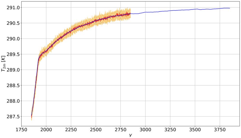
b)

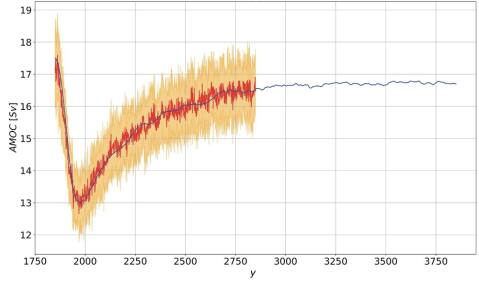
Figure 4: Prediction of a) Globally averaged surface temperature and b) Atlantic Meridional Overturning Circulation (AMOC) strength as a result of an annual 1% increase of the CO₂ concentration from pre-industrial conditions up to doubling. In each panel the blue curve indicates the prediction by application of response theory while the thick red curve shows the ensemble mean of the model runs (yellow curves).) From Lembo2020 .

III.1 Response, Feedbacks, and Koopman Modes

Response theory makes it possible to investigate the key features of the climatic feedbacks acting on different time scales. We provide a rewriting of the Green’s functions in terms of individual components specifically associated with the eigenmodes of the unperturbed Kolmogorov operator $\mathcal{L}_{0}^{\ast}$; see Eq. (28a), Box 4. We assume that $\mathcal{L}_{0}^{\ast}$ has a vanishing eigenvalue $\lambda_{0}=0$ with unitary multiplicity, which is tantamount to assuming a unique invariant measure.

Let $\{\lambda_{j}\}_{j=1}^{M}$ denote the $M$ nonzero eigenvalues of finite algebraic multiplicity $m_{j}$, ordered by their real part in decreasing order, i.e. with $\lambda_{1}$ having the largest real part. The $\lambda_{j}$ are either real or come in complex conjugate pairs. Namely, if $\lambda_{j}$ is an eigenvalue of the unperturbed Kolmogorov operator $\mathcal{L}_{0}^{\ast}$ with eigenfunction $\psi^{\ast}_{j}$, so is $e^{\lambda_{j}t}$ of ${K}_{t}=e^{t\mathcal{L}^{\ast}_{0}}$ relative to the same eigenfunction. With an abuse of language, we shall refer to the $\lambda_{j}$’s and the $\psi^{\ast}_{j}$ as Koopman eigenvalues and Koopman eigenmodes (or simply modes), respectively. These have been introduced in Sec. II.1 for the case of deterministic evolution, we adopt here the same terminology; the Kolmogorov operator being the analogue to the Koopman generator in the stochastic setting Chekroun_al_RP2 . The eigenfunctions $\psi^{\ast}_{j}$ encode the stochastic system’s natural variability, decay of correlations and (temporal) power spectra; see (Chekroun_al_RP2, , Corollary 1 and Sec. 2.3). Koopman analysis and related methods have demonstrated great promises over the last decade in capturing modes of climate variability from high-dimensional model and observational data Froyland2021 .

Following Tantet2018 ; Chekroun_al_RP2 , it was shown in Santos2022 that using the Koopman mode formalism it is possible to express the Green’s functions $\mathcal{G}_{k,p}$ introduced in Eq. (27) as a sum of exponential functions (possibly multiplied by polynomials):

$$\mathcal{G}^{k}_{d/s,\Psi}(t)=\Theta(t)\sum_{j=1}^{{M}}\sum_{\ell=0}^{m_{j}-1}\alpha_{j}^{\ell,k,s/d}(\Psi)\frac{1}{\ell!}e^{\lambda_{j}t}t^{\ell},$$ (29)

where the coefficient $\alpha_{j}^{\ell,k,s/d}(\Psi)$ are discussed in Box 5, whereas their expression can be found in Santos2022 . In Eq. (29) we are neglecting the contribution to the response coming from the essential component of the spectrum of $\mathcal{L}_{0}^{*}$ Santos2022 . Making this important simplifying assumption amounts, by and large, to assuming that the operator $\mathcal{L}_{0}^{*}$ is quasi-compact engel2000 . This is often implicitly assumed when performing extended DMD williams2015data . This derivation explains why the formula presented in Eq. (5) allowed correctly interpreting the climate feedbacks in Maier-Reimer1987 ; Hasselmann1993b . We stress here that the $\lambda_{j}$ do not depend on either the observable or the forcing considered, but are instead a fundamental property of the reference, unperturbed system’s dynamics.

III.2 Tipping Points

Since any Green’s function for the observable $\Psi$ can be interpreted as a correlation function between $\Psi$ and a suitably defined observable $\Phi$ (Box 4), it should not come to a surprise that, considering Eq. (29), one has:

$${\color[rgb]{0,0,0}C_{\Psi_{1},\Psi_{2}}(t)}=\sum_{j=1}^{{M}}\sum_{\ell=0}^{m_{j}-1}\beta_{j}^{\ell,k}(\Psi_{1},\Psi_{2})\frac{1}{\ell!}e^{\lambda_{j}t}t^{\ell},$$ (30)

for any pair of observables $\Psi_{1},\Psi_{2}$, as proved in (Chekroun_al_RP2, , Corollary 1). It is clear from Eqns. (29)-(30) that in order to have a non-explosive behaviour, one must have $\mathfrak{Re}(\lambda_{j})<0$, $1\leq j\leq M$. From Eqns. (29)-(30) it is also clear that the rate of decay of any Green’s function and that of any lagged correlation is dominated for large times by the real part of the subdominant pair of the $\mathcal{L}^{*}_{0}$ spectrum. We refer to $\gamma=\mathfrak{Re}(\lambda_{1})$ as the corresponding spectral gap. The eigenfunctions corresponding to the slowly decaying eigenvalues are the rigorous counterpart of the so-called neutral climate modes Navarra1993 ; Palmer1999 ; Pedram2 ; Lu2020 .

If we assume that say one parameter $\eta$ of our system (not to be confused with $\eta$ in Eq. (14)) is such that the spectral gap $\gamma=\mathfrak{Re}(\lambda_{1})$ vanishes as $\eta\rightarrow\eta_{c}$, we have that as $\eta$ nears it critical value $\eta_{c}$:

• Any Green function and any lagged correlation decays sub-exponentially unless the corresponding factors ($\alpha$’s and $\beta$’s, respectively) vanish;

• Due to the sensitivity formula given in Box 4, one immediately derives that as we near a tipping point, the sensitivity of the system increases in consistency with earlier results linking the smallness of the spectral gap $\gamma$ to sensitivity of the statistics Chek_al14_RP .

These two phenomena—critical slowing down and diverging sensitivity—are key manifestations of the proximity of tipping points Lenton.tip.08 . If the dynamics of the system can be approximated, in a coarse-grained sense, by a Ornstein-Uhlenbeck process such as in PenlandSardeshmukh_JCL95 , another manifestation of getting to close to a tipping point is

• The increase in the signal’s variance Held2004 ; scheffer2012anticipating ; Boettner2022 .

In more general terms, (iii) corresponds to an increased sensitivity of the system to background noise; see Lucarini2012 ; Santos2022 .

The AMOC has long been seen as a climatic subsystem with potential tipping behaviour as a result of changing climatic conditions, and, specifically, of changes in the hydrological cycle and cryosphere in the Atlantic basin Rahmstorf1995 ; Dijkstra2005low ; Kuhlbrodt2007 . Figure 5 shows results from Boers2021 ; caesar2018observed describing signs from observations that support a nearing of the AMOC to a highly plausible critical transition. One finds an increase of the sensitivity and in the variance of an AMOC index tied to the sea surface temperature (SST), as well as by a decrease of the index’ rate of decay; see also (Boers2021, , Fig. 4). Large sensitivity and slow recovery of the same large-scale climate driver has already been discussed in a modelling context in Fig. 4.

We can learn more about such critical behaviour by taking the Fourier transform of the Green’s function given in Eq. (27):

$$\mathfrak{F}\left[\mathcal{G}^{k}_{d/s,\Psi}\right](\omega)=\sum_{j=1}^{M}\sum_{{\color[rgb]{0,0,0}\ell=0}}^{{\color[rgb]{0,0,0}m_{j}}-1}\frac{\alpha_{j}^{\ell,k,s/d}(\Psi)}{\left(i\omega-\lambda_{j}\right)^{{\color[rgb]{0,0,0}\ell+1}}}.$$ (31)

Box 5: Nonequilibrium Oscillator Strengths Equation (31) indicates that the coefficient $\alpha_{j}^{\ell,k,s/d}(\Psi)$ weight the contributions to the frequency-dependent response coming from the eigenmode(s) corresponding to the eigenvalue $\lambda_{j}$ (which has in general multiplicity $m_{j}$) for a given combination of observable and forcing. Note that there is a total of $M=M_{1}+2M_{2}$ eigenvalues. Of these, $M_{1}$ are real, and $M_{2}$ are complex conjugate pairs. Hence, the $\alpha^{\prime}s$ are the non-equilibrium, classical equivalent of the well-known oscillator strengths discussed in spectroscopy, which weight the contributions to the optical susceptibility from each of the allowed quantum transitions from the ground states to the accessible excited states Hilborn1982 ; Lucarini2005 . Thus, Eq. (31) provides the basis for a spectroscopy of general nonequilibrium systems, and, specifically, of the climate system. Resonant terms are associated with tipping phenomena.

The poles of the susceptibility are located at $\omega=-i\lambda_{j}$. Equation  (31) implies the existence of resonances in the response for real frequencies $\omega=\mathfrak{Im}(\lambda_{j})$. Neglecting the possible existence of nonunitary algebraic multiplicities, the susceptibility at the resonance $j$ is proportional to $1/\mathfrak{Re}(\lambda_{j})$. Hence, as $\eta\rightarrow\eta_{c}$, the susceptibility for $\omega=\mathfrak{Im}(\lambda_{1})$ diverges, thus implying a breakdown of the response operator. If at criticality $\mathfrak{Im}(\lambda_{1})=0$, the static response of the system diverges, indicating a saddle-node-like bifurcation phenomenon (turning point). If, instead, $\mathfrak{Im}(\lambda_{1})\neq 0$, we face an oscillatory unstable phenomenon that is reminiscent to a Hopf bifurcation Tantet_al_Hopf ; TantetJSPIII . The viewpoint proposed here allows for linking the fundamental features of the tipping phenomenology within a coherent framework.

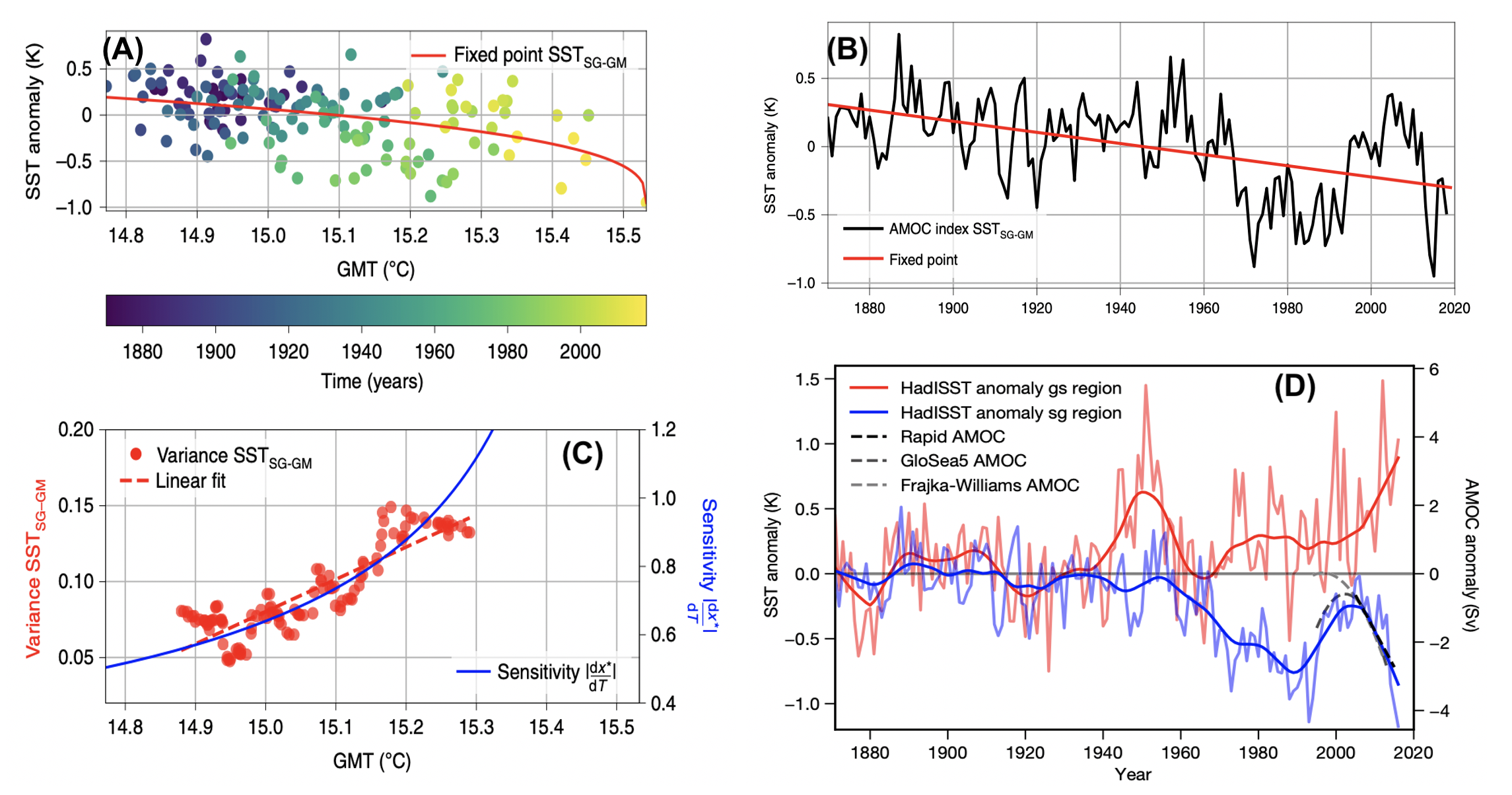
Figure 5: (Adapted from Boers2021 and caesar2018observed ) Panel A: AMOC index SST${}_{\tiny\mbox{SG-GM}}$ caesar2018observed as a function of global mean temperature (GMT) and least-squares fit of the fixed point of a conceptual AMOC model from Boers2021 . Panel B: The SST-based AMOC index SST${}_{\tiny\mbox{SG-GM}}$, constructed by subtracting the global mean SSTs from the average SSTs of the subpolar gyre region (black), supplemented by the same least-squares fit (red) Boers2021 . Panel C: Variance of fluctuations of the AMOC index around the fixed point (red) and corresponding sensitivity of the model, with control parameter $T$ given by the global mean SSTs. These variances are estimated over a sliding temporal window and the results are plotted at the centre point of that window Boers2021 . Panel D: Observational evidence of the nearing of the AMOC tipping point during the last century from caesar2018observed . Shown are time series of SST anomalies with respect to the global mean SST in the subpolar gyre (sg) and the Gulf Stream (gs) regions (HadISST data).

IV Detection and Attribution of Climate Change

The statistical mechanical tools discussed above allow for performing climate change projections for ensembles of trajectories: statements are made in terms of (changes of) the expectation value of general observables. Clearly this is a mathematical construction that does not fully comply with the requirements of climate science, because, as mentioned above, we wish to make statements on the statistical properties of the climate signal we are experiencing—we do not have to access to the hypothetical multiverse comprising of other statistically equivalent realisations—and possibly link it to acting forcing. Nonetheless, linear response theory applied to climate provides solid physical and dynamical foundations for detection and attribution via statistical techniques.

Let $\Psi_{k}$, $k=1,\ldots,N$ be a collection of climatic variables. Consider also the possibility that the forcing to the climate system comes from $F$ different sources, be them anthropogenic or natural. We rewrite Eq. (26) by clamping together all the $U+V=F$ acting forcings as $\delta^{(1)}[\Psi_{k}](t)=\sum_{p=1}^{F}\varepsilon_{p}\left(g_{p}\bullet\mathcal{G}_{p,k}\right)(t)$. Hence we have that, at first order,

$$Y_{k}(t)=\Psi_{k}(t)-\langle\Psi_{k}\rangle_{0}=\sum_{p=1}^{F}\tilde{X}_{k}^{p}(t)+\mathcal{R}_{k}(t),$$ (32)

where $\Psi_{k}(t)$ indicates the actual value of the climate variable $\Psi_{k}$ at time $t$, the terms $\tilde{X}_{k}^{p}(t)=\varepsilon_{p}\left(g_{p}\bullet\mathcal{G}_{p,k}\right)(t)$ account for the forced variability, and $\mathcal{R}_{k}(t)=\Psi_{k}(t)-\langle\Psi\rangle_{\rho_{\varepsilon}^{t}}$ is a random vector whose correlations are governed by the probability distribution $\rho_{\varepsilon}^{t}$ solving the FPE associated with Eq. (25). If the variables $\Psi_{k}$ correspond to anomalies with respect to the reference climatology, we have $\langle\Psi_{k}\rangle_{0}=0$.

Equation (32) is cast into a form that is very close to the usual mathematical formulation of optimal fingerprinting for climate change given in Eq. (6). Response theory indicates that if we use the forced run of a model to perform detection and attribution of climate change as simulated by the same model, and if we are in the linear regime of response, all the $\beta_{p}$’s should be unitary, apart from uncertainty.

We stress that the linear response theory indicates that the optimal fingerprinting procedure could be applied seamlessly for different time horizons of the climate change signal and for suitably linearly filtered signals (e.g. considering time averages). This suggests that one should perform the optimal fingerprinting for different time horizons at the same time, and check the consistency of the obtained results (in terms of confidence intervals for the $\beta$’s) across the time of the hindcast. Additionally, the fact that linear response theory applies for a large class of forcings and can even be adapted for studying extremes LKFW14 explains why optimal fingerprinting finds such a broad range of applications, including the analysis of climatic extremes Naveau2020 ; Wang2021 .

Our derivation emphasizes that optimal fingerprinting relies strongly on assuming linearity in the response, with values of the $\beta$-factors different from unity surrogating in a very simplified manner possibly amplified ($\beta>1$) and damped ($\beta<1$) response due to nonlinear effects. A more accurate treatment of nonlinearities could be achieved by adapting the so-called factor separation method, which is used in meteorology to disentangle linear and nonlinear components of the sensitivity of a system to various acting forcings Stein1993 . Such a method has been recently used for evaluating the factors impacting past climatic conditions Hossain2023 . The consideration of higher order terms in the response operators ruelle_nonequilibrium_1998 could facilitate the development of fingerprinting methods that go beyond the linear approximation. Additionally, it is clear that performing optimal fingerprinting without considering the whole portfolio of acting forcings can lead to misattribution of the causes of detected climate change. The systematic cross-check proposed above for different time horizons might partly take care of these possible criticalities.

The term $\mathcal{R}_{k}(t)$ in Eq. (32) is not associated with the variability of the unperturbed climate—compare with Eq. (6)—but rather is tied to the system’s variability encoded by the probability distribution $\rho_{\epsilon}^{t}$; see also discussions on time-dependent probability measures and pullback attractors in Chekroun2011 ; CLR13 ; CGN17 ; TelJSP ; Tel2020 ; Chekroun_al22SciAdv . This allows us to point out that the classical formulation of optimal fingerprinting lacks the framework to account for changes in variability due to climate change.

The expression for the Green function given in Eq. (29) provides useful information for better understanding the robustness of the optimal fingerprinting method. The model error manifests itself in the difference between the spectrum of eigenvalues (and eigenfunctions) of the Koopman operator of the “real” climate and that of the model used for constructing the fingerprints. Additionally, different climate models will in general feature different Koopman modes and associated eigenvalues. Hence, constructing fingerprints by bundling together information derived from different models seems not so promising in terms of reducing model error.

It is also clear that if only one between the actual climate system and the model used for optimal fingerprinting are close to a tipping point, one expects major uncertainties and biases because of the qualitative mismatch between the leading $j=1$ term of all the involved Green functions, and, hence, between the model fingerprints and the actual climatic response to the considered forcings. This becomes even more critical if more models are used for estimating of the fingerprints, because heavily spurious information could be could added.

V Discussion

The Hasselmann program has had a great influence in the modern development of climate science, both regarding its everyday practice and its more foundational aspects. The fundamental idea boils down to treating noise not like a nuisance one needs to filter out to gather useful information, but rather as a key aspect of the climate system one needs to fully explore and appreciate in order to further its understanding and to link model output and observational data. This is key for making progress in detecting and attributing the climate change signals at different spatial and temporal scales.

The emphasis on the role of noise in creating - somewhat counterintuitively - meaningful signal at lower frequencies has led to fundamental discoveries like in the case of the mechanism of stochastic resonance, which stemmed as a direct application of Hasselmann paradigm in a climatic context Benzi1981 ; Nicolis1981 ; Benzi1982 ; Nicolis1982 but has since had huge success in a plethora of other research areas gammaitoni1998 . Another important area of application of Hasselmann paradigm deals with one of the age-old problems of dynamical meteorology: the fast atmospheric processes due to baroclinic disturbances have been interpreted as acting as effective noise responsible for the low-frequency variability of the mid-latitudes due with the transitions betweeen competing regimes of circulations, mainly associated with zonal flow and blockings, respectively Charney1979 ; Benzi1986 ; Benzi1989 ; Kimoto1993a ; Itoh.Kimoto.1996 .

The (joint) analysis of climate variability and climate response presented here assumes that we are considering forced or free fluctuations around a stable, balanced state, where overall negative feedbacks dominate and control the relaxation processes. Yet, the very concept of balance might need a critical appraisal when considering ultralong time scales Arnscheidt2022Balance , because the internal feedbacks of the system can change sign when different characteristic time scales are considered Arnscheidt2022Feedbacks . The prevalence of positive feedbacks indicate processes associated with transitions between possibly radically different climatic regimes Rothman2017 ; GhilLucarini2020 . Also in this case the stochastic climate modelling angle shows great potential. Taking advantage of Fredilin-Wentzell theory of noise-induced escapes from attractors freidlin1998 and of large deviation theory T09 , it is possible to develop a theory of metastability for geophysical flows Bouchet2012 ; Herbert2015 and for the climate system LucariniBodai2019PRL ; LucariniBodai2020 ; Margazoglou2021 ; Rousseau2023 . While gaussian noise is often used in many investigations for reasons of practical and theoretical convenience, more general classes of noise laws—specifically $\alpha$-stable Lévy processes—are sometimes invoked for studying climatic transitions where sudden jumps between competing states are observed Ditlevsen1999 ; penland_levy ; Gottwald2021 ; LucariniSM2022 . For reasons of space and internal coherence, we have chosen not to cover these important research areas in this review.

The Hasselmann program, by construction, leaves out the problem of finding the root causes of the noise that impacts the slow climatic variables. In this sense, it can be seen as proposing a phenomenological theory of climate. As well known, the noise comes from the fast fluid dynamical instabilities occurring at different scales, in the atmosphere and in the ocean, leading to chaotic behaviour GhilChildress1987 ; Ghil.2019 ; GhilLucarini2020 . The details of the fast processes, in fact, do matter, exactly because there is no time separation one can use to separate the variables of interest from those one wants to parametrize, so that the kind of parsimony one would derive from the use of homogeneization theory cannot be recovered pavliotisbook2014 . On the other hand, there is no dichotomy between deterministic behaviour and stochastic representation, because chaos generates stochastic processes. In order to advance in the direction of constructing a theory of climate able to account for variability and response to forcing, and able to provide useful and usable information to address the climate crisis, there is need to inform the stochastic angle on climate with the key details obtained by a multiscale analysis of the dynamical processes. This review is a preliminary attempt to go in this direction.

References

- (1) J. P. Peixoto and A. H. Oort, Physics of Climate. New York: AIP Press, 1992.
- (2) V. Lucarini, R. Blender, C. Herbert, F. Ragone, S. Pascale, and J. Wouters, “Mathematical and physical ideas for climate science,” Rev. Geophys., vol. 52, no. 4, pp. 809–859, 2014.
- (3) J. Mitchell, “An overview of climatic variability and its causal mechanisms,” Quaternary Research, vol. 6, no. 4, pp. 481–493, 1976.
- (4) M. Ghil, “A century of nonlinearity in the geosciences,” Earth and Space Science, vol. 6, pp. 1007–1042, 2019.
- (5) A. S. von der Heydt, P. Ashwin, C. D. Camp, M. Crucifix, H. A. Dijkstra, P. Ditlevsen, and T. M. Lenton, “Quantification and interpretation of the climate variability record,” Global and Planetary Change, vol. 197, p. 103399, 2021.
- (6) D. H. Rothman, “Thresholds of catastrophe in the earth system,” Science Advances, vol. 3, no. 9, p. e1700906, 2017.
- (7) C. W. Arnscheidt and D. H. Rothman, “Presence or absence of stabilizing earth system feedbacks on different time scales,” Science Advances, vol. 8, no. 46, p. eadc9241, 2022.
- (8) M. Ghil and V. Lucarini, “The physics of climate variability and climate change,” Reviews of Modern Physics, 2020.
- (9) M. Ghil, “A mathematical theory of climate sensitivity or, How to deal with both anthropogenic forcing and natural variability?,” in Climate Change : Multidecadal and Beyond (C. P. Chang, M. Ghil, M. Latif, and J. M. Wallace, eds.), pp. 31–51, World Scientific Publishing Co./Imperial College Press, 2015.
- (10) J. Pearl, Probabilistic reasoning in intelligent systems : networks of plausible inference. San Francisco, Calif.: Morgan Kaufmann, 2009. Example for Explaning away.
- (11) K. Hasselmann, “Optimal fingerprints for the detection of time-dependent climate change,” Journal of Climate, vol. 6, no. 10, pp. 1957 – 1971, 1993.
- (12) G. C. Hegerl, H. von Storch, K. Hasselmann, B. D. Santer, U. Cubasch, and P. D. Jones, “Detecting greenhouse-gas-induced climate change with an optimal fingerprint method,” Journal of Climate, vol. 9, no. 10, pp. 2281 – 2306, 1996.
- (13) K. Hasselmann, “Multi-pattern fingerprint method for detection and attribution of climate change,” Climate Dynamics, vol. 13, no. 9, pp. 601–611, 1997.
- (14) N. L. Bindoff, P. A. Stott, K. M. AchutaRao, M. R. Allen, N. Gillett, D. Gutzler, K. Hansingo, G. Hegerl, Y. Hu, S. Jain, I. I. Mokhov, J. Overland, J. Perlwitz, R. Sebbari, and X. Zhang, Detection and attribution of climate change: From global to regional, pp. 867–952. Cambridge, UK: Cambridge University Press, 2013.
- (15) IPCC, Climate Change 2021: The Physical Science Basis. Contribution of Working Group I to the Sixth Assessment Report of the Intergovernmental Panel on Climate Change, vol. In Press. Cambridge, United Kingdom and New York, NY, USA: Cambridge University Press, 2021.
- (16) IPCC, Managing the Risks of Extreme Events and Disasters to Advance Climate Change Adaptation. A Special Report of Working Groups I and II of the Intergovernmental Panel on Climate Change. Cambridge and New York: Cambridge University Press, 2012.
- (17) T. Lenton, H. Held, E. Kriegler, J. Hall, W. Lucht, S. Rahmstorf, and H. Schellnhuber, “Tipping elements in the {Earth’s climate system},” Proc. Natl. Acad. Sci. USA, vol. 105, pp. 1786–1793, 2008.
- (18) P. Ashwin, S. Wieczorek, R. Vitolo, and P. Cox, “Tipping points in open systems: Bifurcation, noise-induced and rate-dependent examples in the climate system,” Philosophical Transactions of the Royal Society A: Mathematical, Physical and Engineering Sciences, vol. 370, no. 1962, pp. 1166–1184, 2012.
- (19) W. J. Ripple, C. Wolf, T. M. Newsome, J. W. Gregg, T. M. Lenton, I. Palomo, J. A. J. Eikelboom, B. E. Law, S. Huq, P. B. Duffy, and J. Rockström, “World Scientists’ Warning of a Climate Emergency 2021,” BioScience, vol. 71, pp. 894–898, 07 2021.
- (20) P. Imkeller and J. S. von Storch, Stochastic Climate Models. Basel: Birkhauser, 2001.
- (21) H. von Storch, From Decoding Turbulence to Unveiling the Fingerprint of Climate Change. New York: Springer Cham, 2022.
- (22) S. Gupta, N. Mastrantonas, C. Masoller, and J. Kurths, “Perspectives on the importance of complex systems in understanding our climate and climate change—The Nobel Prize in Physics 2021,” Chaos: An Interdisciplinary Journal of Nonlinear Science, vol. 32, 05 2022. 052102.
- (23) G. C. Hegerl, “Climate change is physics,” Communications Earth & Environment, vol. 3, no. 1, p. 14, 2022.
- (24) K. Hasselmann, “Stochastic climate models Part I. Theory,” Tellus, vol. 28, no. 6, pp. 473–485, 1976.
- (25) L. Arnold, “Hasselmann’s program revisited: the analysis of stochasticity in deterministic climate models,” in Stochastic Climate Models (P. Imkeller and J.-S. von Storch, eds.), (Basel), pp. 141–157, Birkhäuser Basel, 2001.
- (26) D. Kelly and I. Melbourne, “Deterministic homogenization for fast-slow systems with chaotic noise,” Journal of Functional Analysis, vol. 272, no. 10, pp. 4063–4102, 2017.
- (27) C. J. Cotter, G. A. Gottwald, and D. D. Holm, “Stochastic partial differential fluid equations as a diffusive limit of deterministic Lagrangian multi-time dynamics,” Proceedings of the Royal Society A: Mathematical, Physical and Engineering Sciences, vol. 473, no. 2205, p. 20170388, 2017.
- (28) M. Ghil and S. Childress, Topics in Geophysical Fluid Dynamics: Atmospheric Dynamics, Dynamo Theory, and Climate Dynamics. Berlin: Springer-Verlag, 1987.
- (29) E. Lorenz, The Nature and Theory of the General Circulation of the Atmosphere. Geneva, Switzerland: World Meteorological Organization, 1967.
- (30) C. Beck, “Brownian motion from deterministic dynamics,” Physica A: Statistical Mechanics and its Applications, vol. 169, no. 2, pp. 324–336, 1990.
- (31) W. Just, H. Kantz, C. Rödenbeck, and M. Helm, “Stochastic modelling: replacing fast degrees of freedom by noise,” Journal of Physics A: Mathematical and General, vol. 34, no. 15, pp. 3199–3213, 2001.
- (32) A. J. Majda, I. Timofeyev, and E. Vanden-Eijnden, “A mathematical framework for stochastic climate models,” Comm. Pure Appl. Math, vol. 54, no. 8, pp. 891–974, 2001.
- (33) G. A. Pavliotis and A. M. Stuart, Multiscale Methods. New York: Springer, 2008.
- (34) G. A. Gottwald and I. Melbourne, “Homogenization for deterministic maps and multiplicative noise,” Proceedings of the Royal Society A: Mathematical, Physical and Engineering Sciences, vol. 469, no. 2156, p. 20130201, 2013.
- (35) R. Khasminsky, “Principle of averaging for parabolic and elliptic differential equations and for Markov processes with small diffusion,” Theory of Probability & Its Applications, vol. 8, no. 1, pp. 1–21, 1963.
- (36) T. Kurtz, “A limit theorem for perturbed operator semigroups with applications to random evolutions,” Journal of Functional Analysis, vol. 12, no. 1, pp. 55–67, 1973.
- (37) G. C. Papanicolaou and W. Kohler, “Asymptotic theory of mixing stochastic ordinary differential equations,” Communications on Pure and Applied Mathematics, vol. 27, no. 5, pp. 641–668, 1974.
- (38) A. J. Majda, I. Timofeyev, and E. Vanden-Eijnden, “Systematic strategies for stochastic mode reduction in climate,” J. Atmos. Sci., vol. 60, no. 14, pp. 1705–1722, 2003.
- (39) T. N. Palmer and P. Williams, eds., Stochastic Physics and Climate Modelling. Cambridge: Cambridge University Press, nov 2009.
- (40) J. Berner, U. Achatz, L. Batté, L. Bengtsson, A. de la Cámara, H. M. Christensen, M. Colangeli, D. R. B. Coleman, D. Crommelin, S. I. Dolaptchiev, and C. L. Franzke, “Stochastic parameterization: {Toward a new view of weather and climate models},” Bulletin of the American Meteorological Society, vol. 98, no. 3, pp. 565–588, 2017.
- (41) M. Chekroun, H. Dijkstra, T. Şengül, and S. Wang, “Transitions of zonal flows in a two-layer quasi-geostrophic ocean model,” Nonlinear Dynamics, vol. 109, no. 3, pp. 1887–1904, 2022.
- (42) H. Dijkstra, Nonlinear physical oceanography: A dynamical systems approach to the large-scale ocean circulation and El Niño, vol. 532. Springer, 2005.
- (43) H. A. Dijkstra and M. Ghil, “Low-frequency variability of the large-scale ocean circulation: A dynamical systems approach,” Reviews of Geophysics, vol. 43, no. 3, p. RG3002, 2005.
- (44) M. D. Chekroun, H. Liu, and S. Wang, Approximation of Stochastic Invariant Manifolds: Stochastic Manifolds for Nonlinear SPDEs I. Springer Briefs in Mathematics, Springer, 2015.
- (45) M. D. Chekroun, H. Liu, and S. Wang, Stochastic Parameterizing Manifolds and Non-Markovian Reduced Equations: Stochastic Manifolds for Nonlinear SPDEs II. Springer Briefs in Mathematics, Springer, 2015.
- (46) M. Chekroun, H. Liu, J. McWilliams, and S. Wang, “Transitions in stochastic non-equilibrium systems: Efficient reduction and analysis,” Journal of Differential Equations, vol. 346, pp. 145–204, 2023.
- (47) J. Wouters and G. A. Gottwald, “Edgeworth expansions for slow-fast systems with finite time-scale separation,” Proceedings of the Royal Society A: Mathematical, Physical and Engineering Sciences, vol. 475, no. 2223, p. 20180358, 2019.
- (48) J. Wouters and G. A. Gottwald, “Stochastic model reduction for slow-fast systems with moderate time scale separation,” Multiscale Modeling & Simulation, vol. 17, no. 4, pp. 1172–1188, 2019.
- (49) G. A. Pavliotis, Stochastic Processes and Applications, vol. 60. Springer, New York, 2014.
- (50) N. Maher, S. Milinski, and R. Ludwig, “Large ensemble climate model simulations: introduction, overview, and future prospects for utilising multiple types of large ensemble,” Earth System Dynamics, vol. 12, no. 2, pp. 401–418, 2021.
- (51) C. W. Arnscheidt and D. H. Rothman, “The balance of nature: A global marine perspective,” Annual Review of Marine Science, vol. 14, no. 1, pp. 49–73, 2022. PMID: 34115541.
- (52) B. Saltzman, Dynamical Paleoclimatology: Generalized Theory of Global Climate Change. New York: Academic Press New York, nov 2001.
- (53) M. Chekroun, A. Tantet, H. Dijkstra, and J. D. Neelin, “Ruelle-Pollicott Resonances of Stochastic Systems in Reduced State Space. Part I: Theory,” J. Stat. Phys., vol. 179, pp. 1366–1402, 2020.
- (54) J.-P. Eckmann and D. Ruelle, “Ergodic theory of chaos and strange attractors,” Rev. Modern Phys., vol. 57, pp. 617–656, 1985.
- (55) S. Bojinski, M. Verstraete, T. C. Peterson, C. Richter, A. Simmons, and M. Zemp, “The concept of essential climate variables in support of climate research, applications, and policy,” Bulletin of the American Meteorological Society, vol. 95, no. 9, pp. 1431 – 1443, 2014.
- (56) V. Eyring, L. Bock, A. Lauer, M. Righi, M. Schlund, B. Andela, E. Arnone, O. Bellprat, B. Brötz, L.-P. Caron, N. Carvalhais, I. Cionni, N. Cortesi, B. Crezee, E. L. Davin, P. Davini, K. Debeire, L. de Mora, C. Deser, D. Docquier, P. Earnshaw, C. Ehbrecht, B. K. Gier, N. Gonzalez-Reviriego, P. Goodman, S. Hagemann, S. Hardiman, B. Hassler, A. Hunter, C. Kadow, S. Kindermann, S. Koirala, N. Koldunov, Q. Lejeune, V. Lembo, T. Lovato, V. Lucarini, F. Massonnet, B. Müller, A. Pandde, N. Pérez-Zanón, A. Phillips, V. Predoi, J. Russell, A. Sellar, F. Serva, T. Stacke, R. Swaminathan, V. Torralba, J. Vegas-Regidor, J. von Hardenberg, K. Weigel, and K. Zimmermann, “Earth system model evaluation tool (esmvaltool) v2.0 – an extended set of large-scale diagnostics for quasi-operational and comprehensive evaluation of earth system models in cmip,” Geoscientific Model Development, vol. 13, no. 7, pp. 3383–3438, 2020.
- (57) E. Maier-Reimer and K. Hasselmann, “Transport and storage of CO2 in the ocean—an inorganic ocean-circulation carbon cycle model,” Climate Dynamics, vol. 2, no. 2, pp. 63–90, 1987.
- (58) K. Hasselmann, R. Sausen, E. Maier-Reimer, and R. Voss, “On the cold start problem in transient simulations with coupled atmosphere-ocean models,” Climate Dynamics, vol. 9, no. 2, pp. 53–61, 1993.
- (59) C. Leith, “Climate response and fluctuation dissipation,” Journal of the Atmospheric Sciences, vol. 32, no. 10, pp. 2022–2026, 1975.
- (60) R. Kubo, “The fluctuation-dissipation theorem,” Reports on Progress in Physics, vol. 29, no. 1, pp. 255–284, 1966.
- (61) T. Tél, T. Bódai, G. Drótos, T. Haszpra, M. Herein, B. Kaszás, and M. Vincze, “The theory of parallel climate realizations,” Journal of Statistical Physics, vol. 179, no. 5, pp. 1496–1530, 2020.
- (62) A. Hannart, A. Ribes, and P. Naveau, “Optimal fingerprinting under multiple sources of uncertainty,” Geophysical Research Letters, vol. 41, no. 4, pp. 1261–1268, 2014.
- (63) M. Allen and S. Tett, “Checking for model consistency in optimal fingerprinting,” Climate Dynamics, vol. 15, pp. 419–434, 06 1999.
- (64) M. Allen and S. Tett, “Estimating signal amplitudes in optimal fingerprinting, part i: theory,” Climate Dynamics, vol. 21, no. 5, pp. 477–491, 2003.
- (65) G. Hegerl and F. Zwiers, “Use of models in detection and attribution of climate change,” Wiley interdisciplinary reviews: climate change, vol. 2, no. 4, pp. 570–591, 2011.
- (66) Y. Li, K. Chen, J. Yan, and X. Zhang, “Uncertainty in optimal fingerprinting is underestimated,” Environmental Research Letters, vol. 16, p. 084043, aug 2021.
- (67) R. McKitrick, “Checking for model consistency in optimal fingerprinting: a comment,” Climate Dynamics, vol. 58, no. 1, pp. 405–411, 2022.
- (68) H. Chen, S. X. Chen, and M. Mu, “A review on the optimal fingerprinting approach in climate change studies,” 2022.
- (69) H. Mori, “Transport, Collective Motion, and Brownian Motion,” Progress of Theoretical Physics, vol. 33, pp. 423–455, mar 1965.
- (70) R. Zwanzig, “Memory effects in irreversible thermodynamics,” Physical Review, vol. 124, no. 4, pp. 983–992, 1961.
- (71) A. J. Chorin, O. H. Hald, and R. Kupferman, “Optimal prediction with memory,” Physica D, vol. 166, no. 3, pp. 239–257, 2002.
- (72) D. Givon, R. Kupferman, and A. Stuart, “Extracting macroscopic dynamics: model problems and algorithms,” Nonlinearity, vol. 17, no. 6, pp. R55–R127, 2004.
- (73) D. Ruelle, “General linear response formula in statistical mechanics, and the fluctuation-dissipation theorem far from equilibrium,” Physics Letters, Section A: General, Atomic and Solid State Physics, vol. 245, no. 3-4, pp. 220–224, 1998.
- (74) D. Ruelle, “A review of linear response theory for general differentiable dynamical systems,” Nonlinearity, vol. 22, no. 4, pp. 855–870, 2009.
- (75) M. Hairer and A. J. Majda, “A simple framework to justify linear response theory,” Nonlinearity, vol. 23, no. 4, pp. 909–922, 2010.
- (76) M. Baiesi and C. Maes, “An update on the nonequilibrium linear response,” New Journal of Physics, vol. 15, p. 013004, jan 2013.
- (77) A. Sarracino and A. Vulpiani, “On the fluctuation-dissipation relation in non-equilibrium and non-hamiltonian systems,” Chaos, vol. 29, p. 083132, 2019.
- (78) G. A. Gottwald, “Introduction to Focus Issue: Linear response theory: Potentials and limits,” Chaos: An Interdisciplinary Journal of Nonlinear Science, vol. 30, no. 2, p. 20401, 2020.
- (79) M. Santos Gutiérrez and V. Lucarini, “On some aspects of the response to stochastic and deterministic forcings,” Journal of Physics A: Mathematical and Theoretical, vol. 55, p. 425002, oct 2022.
- (80) F. Ragone, V. Lucarini, and F. Lunkeit, “A new framework for climate sensitivity and prediction: a modelling perspective,” Climate Dynamics, vol. 46, no. 5, pp. 1459–1471, 2016.
- (81) V. Lucarini, F. Ragone, and F. Lunkeit, “Predicting Climate Change Using Response Theory: Global Averages and Spatial Patterns,” Journal of Statistical Physics, vol. 166, pp. 1036–1064, feb 2017.
- (82) M. Aengenheyster, Q. Y. Feng, F. van der Ploeg, and H. A. Dijkstra, “The point of no return for climate action: effects of climate uncertainty and risk tolerance,” Earth System Dynamics, vol. 9, no. 3, pp. 1085–1095, 2018.
- (83) V. Lembo, V. Lucarini, and F. Ragone, “Beyond Forcing Scenarios: Predicting Climate Change through Response Operators in a Coupled General Circulation Model,” Scientific Reports, vol. 10, no. 1, p. 8668, 2020.
- (84) I. Mezić, “Spectral properties of dynamical systems, model reduction and decompositions,” Nonlinear Dynamics, vol. 41, no. 1, pp. 309–325, 2005.
- (85) M. Budišić, R. Mohr, and I. Mezić, “Applied koopmanism,” Chaos, vol. 22, no. 4, p. 047510, 2012.
- (86) J. Kutz, S. Brunton, B. Brunton, and J. Proctor, Dynamic Mode Decomposition: Data-Driven Modeling of Complex Systems. Other Titles in Applied Mathematics, Philadelphia: Society for Industrial and Applied Mathematics, 2016.
- (87) A. Tantet, V. Lucarini, and H. A. Dijkstra, “Resonances in a Chaotic Attractor Crisis of the Lorenz Flow,” Journal of Statistical Physics, vol. 170, no. 3, pp. 584–616, 2018.
- (88) M. D. Chekroun and N. E. Glatt-Holtz, “Invariant measures for dissipative dynamical systems: Abstract results and applications,” Commun. Math. Phys., vol. 316, pp. 723–761, 2012.
- (89) L. Ambrosio, N. Gigli, and G. Savaré, Gradient Flows in Metric Spaces and in the Space of Probability Measures. Springer Science & Business Media, 2008.
- (90) A. Chorin and O. Hald, Stochastic Tools in Mathematics and Science. No. 147 in Surveys and Tutorials in the Applied Mathematical Sciences, Springer New York, 2006.
- (91) G. Vissio and V. Lucarini, “Evaluating a stochastic parametrization for a fast-slow system using the Wasserstein distance,” Nonlinear Processes in Geophysics, vol. 25, no. 2, pp. 413–427, 2018.
- (92) C. Hijón, P. Español, E. Vanden-Eijnden, and R. Delgado-Buscalioni, “Mori–zwanzig formalism as a practical computational tool,” Faraday discussions, vol. 144, pp. 301–322, 2010.
- (93) S. Izvekov and G. Voth, “Modeling real dynamics in the coarse-grained representation of condensed phase systems,” The Journal of Chemical Physics, vol. 125, no. 15, p. 151101, 2006.
- (94) M. Chen, X. Li, and C. Liu, “Computation of the memory functions in the generalized Langevin models for collective dynamics of macromolecules,” The Journal of Chemical Physics, vol. 141, no. 6, p. 064112, 2014.
- (95) L. Ma, X. Li, and C. Liu, “The derivation and approximation of coarse-grained dynamics from Langevin dynamics,” The Journal of chemical physics, vol. 145, no. 20, p. 204117, 2016.
- (96) M. D. Chekroun, D. Kondrashov, and M. Ghil, “Predicting stochastic systems by noise sampling, and application to the El Niño-Southern Oscillation,” Proc. Natl. Acad. Sci. USA, vol. 108, no. 29, pp. 11766–11771, 2011.
- (97) A. J. Majda and J. Harlim, “Physics constrained nonlinear regression models for time series,” Nonlinearity, vol. 26, no. 1, pp. 201–217, 2013.
- (98) J. Wouters and V. Lucarini, “Multi-level dynamical systems: Connecting the Ruelle response theory and the Mori-Zwanzig approach,” Journal of Statistical Physics, vol. 151, no. 5, pp. 850–860, 2013.
- (99) M. Ghil, M. Chekroun, and G. Stepan, “A collection on ’Climate dynamics: multiple scales and memory effects’,” 2015.
- (100) D. Kondrashov, M. D. Chekroun, and M. Ghil, “Data-driven non-Markovian closure models,” Physica D., vol. 297, pp. 33–55, 2015.
- (101) M. D. Chekroun and D. Kondrashov, “Data-adaptive harmonic spectra and multilayer Stuart-Landau models,” Chaos, vol. 27, no. 9, p. 093110, 2017.
- (102) N. Boers, M. D. Chekroun, H. Liu, D. Kondrashov, D.-D. Rousseau, A. Svensson, M. Bigler, and M. Ghil, “Inverse stochastic-dynamic models for high-resolution Greenland ice-core records,” Earth System Dynamics, vol. 8, pp. 1171–1190, 2017.
- (103) S. Falkena, C. Quinn, J. Sieber, J. Frank, and H. Dijkstra, “Derivation of delay equation climate models using the Mori-Zwanzig formalism,” Proceedings of the Royal Society A, vol. 475, no. 2227, p. 20190075, 2019.
- (104) E. J. Parish and K. Duraisamy, “A dynamic subgrid scale model for Large Eddy Simulations based on the Mori–Zwanzig formalism,” Journal of Computational Physics, vol. 349, pp. 154–175, 2017.
- (105) E. Parish and K. Duraisamy, “Non-Markovian closure models for large eddy simulations using the Mori-Zwanzig formalism,” Physical Review Fluids, vol. 2, no. 1, p. 014604, 2017.
- (106) Q. Wang, N. Ripamonti, and J. S. Hesthaven, “Recurrent neural network closure of parametric POD-Galerkin reduced-order models based on the Mori-Zwanzig formalism,” Journal of Computational Physics, vol. 410, p. 109402, 2020.
- (107) I. Miyadera, “On perturbation theory for semi-groups of operators,” Tohoku Mathematical Journal, Second Series, vol. 18, no. 3, pp. 299–310, 1966.
- (108) J. Voigt, “On the perturbation theory for strongly continuous semigroups,” Mathematische Annalen, vol. 229, no. 2, pp. 163–171, 1977.
- (109) K.-J. Engel and R. Nagel, One-Parameter Semigroups for Linear Evolution Equations. New York: Springer-Verlag, 2000.
- (110) D. Givon, R. Kupferman, and O. Hald, “Existence proof for orthogonal dynamics and the Mori-Zwanzig formalism,” Israel Journal of Mathematics, vol. 145, pp. 221–241, 2005.
- (111) P. Stinis, “Higher order Mori-Zwanzig models for the Euler equations,” Multiscale Model. & Simul., vol. 6, no. 3, pp. 741–760, 2007.
- (112) Z. Li, X. Bian, X. Li, and G. Karniadakis, “Incorporation of memory effects in coarse-grained modeling via the Mori-Zwanzig formalism,” The Journal of Chemical Physics, vol. 143, no. 24, p. 243128, 2015.
- (113) H. Lei, N. Baker, and X. Li, “Data-driven parameterization of the generalized langevin equation,” Proceedings of the National Academy of Sciences, vol. 113, no. 50, pp. 14183–14188, 2016.
- (114) Z. Li, H. Lee, E. Darve, and G. Karniadakis, “Computing the non-Markovian coarse-grained interactions derived from the Mori–Zwanzig formalism in molecular systems: application to polymer melts,” The Journal of chemical physics, vol. 146, no. 1, p. 014104, 2017.
- (115) C. Brennan and D. Venturi, “Data-driven closures for stochastic dynamical systems,” Journal of Computational Physics, vol. 372, pp. 281–298, 2018.
- (116) A. J. Chorin and F. Lu, “Discrete approach to stochastic parametrization and dimension reduction in nonlinear dynamics,” Proc. Natl. Acad. Sci. USA, vol. 112, no. 32, pp. 9804–9809, 2015.
- (117) F. Lu, K. K. Lin, and A. J. Chorin, “Data-based stochastic model reduction for the Kuramoto-Sivashinsky equation,” Physica D, vol. 340, pp. 46–57, 2017.
- (118) K. K. Lin and F. Lu, “Data-driven model reduction, Wiener projections, and the Koopman-Mori-Zwanzig formalism,” Journal of Computational Physics, vol. 424, p. 109864, jan 2021.
- (119) J. Harlim, S. Jiang, S. Liang, and H. Yang, “Machine learning for prediction with missing dynamics,” Journal of Computational Physics, vol. 428, p. 109922, 2021.
- (120) D. Qi and J. Harlim, “A data-driven statistical-stochastic surrogate modeling strategy for complex nonlinear non-stationary dynamics,” Journal of Computational Physics, vol. 485, p. 112085, 2023.
- (121) F. Gilani, D. Giannakis, and J. Harlim, “Kernel-based prediction of non-Markovian time series,” Physica D., vol. 418, p. 132829, 2021.
- (122) H. Mori, “A continued-fraction representation of the time-correlation functions,” Progress of Theoretical Physics, vol. 34, no. 3, pp. 399–416, 1965.
- (123) M. Lee, “Solutions of the generalized Langevin equation by a method of recurrence relations,” Physical Review B, vol. 26, no. 5, p. 2547, 1982.
- (124) J. Florencio Jr and M. H. Lee, “Exact time evolution of a classical harmonic-oscillator chain,” Physical Review A, vol. 31, no. 5, p. 3231, 1985.
- (125) R. Kupferman, “Fractional kinetics in Kac–Zwanzig heat bath models,” Journal of Statistical Physics, vol. 114, pp. 291–326, 2004.
- (126) A. J. Chorin, O. H. Hald, and R. Kupferman, “Optimal prediction with memory,” Physica D: Nonlinear Phenomena, vol. 166, no. 3-4, pp. 239–257, 2002.
- (127) A. Chorin and P. Stinis, “Problem reduction, renormalization, and memory,” Com. Appl. Math. Comp. Sci., vol. 1, no. 1, pp. 1–27, 2007.
- (128) P. Stinis, “A comparative study of two stochastic mode reduction methods,” Physica D, vol. 213, no. 2, pp. 197–213, 2006.
- (129) W. Götze, “Recent tests of the mode-coupling theory for glassy dynamics,” Journal of Physics: condensed matter, vol. 11, no. 10A, p. A1, 1999.
- (130) D. Reichman and P. Charbonneau, “Mode-coupling theory,” Journal of Statistical Mechanics: Theory and Experiment, vol. 2005, no. 05, p. P05013, 2005.
- (131) E. Darve, J. Solomon, and A. Kia, “Computing generalized Langevin equations and generalized Fokker–Planck equations,” Proceedings of the National Academy of Sciences, vol. 106, no. 27, pp. 10884–10889, 2009.
- (132) P. Stinis, “Renormalized Mori-Zwanzig-reduced models for systems without scale separation,” Proceedings of the Royal Society A: Mathematical, Physical and Engineering Sciences, vol. 471, no. 2176, p. 20140446, 2015.
- (133) Y. Zhu, J. Dominy, and D. Venturi, “On the estimation of the Mori-Zwanzig memory integral,” Journal of Mathematical Physics, vol. 59, no. 10, p. 103501, 2018.
- (134) Y. Zhu and D. Venturi, “Faber approximation of the Mori–Zwanzig equation,” Journal of Computational Physics, vol. 372, pp. 694–718, 2018.
- (135) D. Venturi and G. Karniadakis, “Convolutionless Nakajima-Zwanzig equations for stochastic analysis in nonlinear dynamical systems,” Proceedings of the Royal Society A: Mathematical, Physical and Engineering Sciences, vol. 470, no. 2166, p. 20130754, 2014.
- (136) J. Wouters and V. Lucarini, “Disentangling multi-level systems: averaging, correlations and memory,” J. Stat. Mech., p. P03003, 2012.
- (137) Y. Yoshimoto, I. Kinefuchi, T. Mima, A. Fukushima, T. Tokumasu, and S. Takagi, “Bottom-up construction of interaction models of non-Markovian dissipative particle dynamics,” Physical Review E, vol. 88, no. 4, p. 043305, 2013.
- (138) J. Demaeyer and S. Vannitsem, “Comparison of stochastic parameterizations in the framework of a coupled ocean–atmosphere model,” Nonlinear Processes in Geophysics, vol. 25, no. 3, pp. 605–631, 2018.
- (139) G. Vissio and V. Lucarini, “A proof of concept for scale-adaptive parametrizations: the case of the Lorenz ’96 model,” Quarterly Journal of the Royal Meteorological Society, vol. 144, no. 710, pp. 63–75, 2018.
- (140) O. H. Hald and P. Stinis, “Optimal prediction and the rate of decay for solutions of the Euler equations in two and three dimensions,” Proc. Natl. Acad. Sci. USA, vol. 104, no. 16, pp. 6527–6532, 2007.
- (141) M. D. Chekroun, F. Di Plinio, N. E. Glatt-Holtz, and V. Pata, “Asymptotics of the Coleman-Gurtin model,” Discrete Contin. Dyn. Syst. Ser. S, vol. 4, no. 2, pp. 351–369, 2011.
- (142) M. D. Chekroun and N. E. Glatt-Holtz, “Invariant measures for dissipative dynamical systems: abstract results and applications,” Commun. Math. Phys., vol. 316, no. 3, pp. 723–761, 2012.
- (143) S. Kravtsov, D. Kondrashov, and M. Ghil, “Multilevel regression modeling of nonlinear processes: Derivation and applications to climatic variability,” Journal of Climate, vol. 18, no. 21, pp. 4404–4424, 2005.
- (144) M. D. Chekroun, H. Liu, and J. C. McWilliams, “Variational approach to closure of nonlinear dynamical systems: Autonomous case,” J. Stat. Phys., vol. 179, pp. 1073–1160, 2020.
- (145) C. Ma, J. Wang, and E. Weinan, “Model reduction with memory and the machine learning of dynamical systems,” Communications in Computational Physics, vol. 25, no. 4, pp. 947–962, 2019.
- (146) V. I. Arnold, Geometrical Methods in the Theory of Ordinary Differential Equations. Springer-Verlag, New York, second ed., 1988.
- (147) M. D. Chekroun, H. Liu, and J. C. McWilliams, “Optimal Parameterizing Manifolds for Anticipating Tipping Points and Higher-order Critical Transitions,” arXiv preprint 2307.06537, https://arxiv.org/abs/2307.06537, 2023.
- (148) A. Debussche and R. Temam, “Inertial manifolds and the slow manifolds in meteorology,” Differential and Integral Equations, vol. 4, no. 5, pp. 897–931, 1991.
- (149) R. Temam and D. Wirosoetisno, “Slow manifolds and invariant sets of the primitive equations,” J. Atmos. Sci., vol. 68, no. 3, pp. 675–682, 2011.
- (150) S. Zelik, “Inertial manifolds and finite-dimensional reduction for dissipative PDEs,” Proc. R. Soc. Edinb. Sec. A: Mathematics, vol. 144, no. 6, pp. 1245–1327, 2014.
- (151) R. H. Kraichnan, “Eddy viscosity in two and three dimensions,” J. Atmos. Sci., vol. 33, no. 8, pp. 1521–1536, 1976.
- (152) C. E. Leith, “Stochastic backscatter in a subgrid-scale model: Plane shear mixing layer,” Physics of Fluids A: Fluid Dynamics, vol. 2, no. 3, pp. 297–299, 1990.
- (153) A. Debussche, T. Dubois, and R. Temam, “The nonlinear Galerkin method: a multiscale method applied to the simulation of homogeneous turbulent flows,” Theoretical and Computational Fluid Dynamics, vol. 7, no. 4, pp. 279–315, 1995.
- (154) T. Dubois, F. Jauberteau, and R. Temam, “Incremental unknowns, multilevel methods and the numerical simulation of turbulence,” Computer Meth. Appl. Mech. Engineering, vol. 159, no. 1-2, pp. 123–189, 1998.
- (155) T. Dubois and F. Jauberteau, “A dynamic multilevel model for the simulation of the small structures in homogeneous isotropic turbulence,” Journal of scientific computing, vol. 13, no. 3, pp. 323–367, 1998.
- (156) X. Fu, L.-B. Chang, and D. Xiu, “Learning reduced systems via deep neural networks with memory,” Journal of Machine Learning for Modeling and Computing, vol. 1, no. 2, 2020.
- (157) A. Gupta and P. F. J. Lermusiaux, “Neural closure models for dynamical systems,” Proceedings of the Royal Society A, vol. 477, no. 2252, p. 20201004, 2021.
- (158) R. H. Kraichnan, “Eddy viscosity and diffusivity: Exact formulas and approximations,” Complex Systems, vol. 1, no. 4-6, pp. 805–820, 1987.
- (159) H. A. Rose, “Eddy diffusivity, eddy noise and subgrid-scale modelling,” Journal of Fluid Mechanics, vol. 81, no. 4, pp. 719–734, 1977.
- (160) D. Kondrashov, S. Kravtsov, A. W. Robertson, and M. Ghil, “A hierarchy of data-based ENSO models,” vol. 18, pp. 4425–4444, 2005.
- (161) M. D. Chekroun, D. Kondrashov, and M. Ghil, “Predicting stochastic systems by noise sampling, and application to the El Niño-Southern Oscillation,” Proceedings of the National Academy of Sciences, vol. 108, no. 29, pp. 11766–11771, 2011.
- (162) C. Chen, M. A. Cane, N. Henderson, D. E. Lee, D. Chapman, D. Kondrashov, and M. D. Chekroun, “Diversity, nonlinearity, seasonality, and memory effect in ENSO simulation and prediction using empirical model reduction,” Journal of Climate, vol. 29, no. 5, pp. 1809–1830, 2016.
- (163) D. Kondrashov, S. Kravtsov, and M. Ghil, “Empirical mode reduction in a model of extratropical low-frequency variability,” vol. 63, pp. 1859–1877, 2006.
- (164) D. Kondrashov, M. D. Chekroun, A. W. Robertson, and M. Ghil, “Low-order stochastic model and “past-noise forecasting” of the Madden-Julian Oscillation,” vol. 40, pp. 5305–5310, 2013. doi:10.1002/grl.50991.
- (165) N. Chen, A. J. Majda, and D. Giannakis, “Predicting the cloud patterns of the Madden-Julian Oscillation through a low-order nonlinear stochastic model,” Geophysical Research Letters, vol. 41, no. 15, pp. 5612–5619, 2014.
- (166) N. Chen and A. J. Majda, “Predicting the real-time multivariate Madden–Julian oscillation index through a low-order nonlinear stochastic model,” Monthly Weather Review, vol. 143, no. 6, pp. 2148–2169, 2015.
- (167) M. Santos Gutiérrez, V. Lucarini, M. D. Chekroun, and M. Ghil, “Reduced-order models for coupled dynamical systems: Data-driven methods and the Koopman operator,” Chaos, vol. 31, no. 5, p. 053116, 2021.
- (168) C. W. Rowley, I. Mezić, S. Bagheri, P. Schlatter, and D. S. Henningson, “Spectral analysis of nonlinear flows,” Journal of Fluid Mechanics, vol. 641, pp. 115–127, 2009.
- (169) P. J. Schmid, “Dynamic mode decomposition of numerical and experimental data,” Journal of Fluid Mechanics, vol. 656, pp. 5–28, 2010.
- (170) K. Hasselmann, “PIPs and POPs: the reduction of complex dynamical systems using principal interaction and oscillation patterns,” Journal of Geophysical Research, vol. 93, no. D9, pp. 11015–11021, 1988.
- (171) J. H. Tu, C. W. Rowley, D. M. Luchtenburg, S. L. Brunton, and J. N. Kutz, “On dynamic mode decomposition: Theory and applications,” Journal of Computational Dynamics, vol. 1, no. 2, pp. 391–421, 2014.
- (172) M. D. Chekroun, H. Liu, and J. C. McWilliams, “The emergence of fast oscillations in a reduced primitive equation model and its implications for closure theories,” Computers & Fluids, vol. 151, pp. 3–22, 2017.
- (173) E. N. Lorenz, “Attractor sets and quasi-geostrophic equilibrium,” J. Atmos. Sci., vol. 37, no. 8, pp. 1685–1699, 1980.
- (174) M. Chekroun, H. Liu, and J. McWilliams, “Stochastic rectification of fast oscillations on slow manifold closures,” Proc. Natl. Acad. Sci. USA, vol. 118, no. 48, p. e2113650118, 2021.
- (175) B. Bolin, “Numerical forecasting with the barotropic model,” Tellus, vol. 7, no. 1, pp. 27–49, 1955.
- (176) F. Baer and J. J. Tribbia, “On complete filtering of gravity modes through nonlinear initialization,” Monthly Weather Review, vol. 105, no. 12, pp. 1536–1539, 1977.
- (177) B. Machenhauer, “On the dynamics of gravity oscillations in a shallow water model with applications to normal mode initialization,” Beitr. Phys. Atmos, vol. 50, pp. 253–271, 1977.
- (178) R. Daley, “Normal mode initialization,” Reviews of Geophysics, vol. 19, no. 3, pp. 450–468, 1981.
- (179) C. Leith, “Nonlinear normal mode initialization and quasi-geostrophic theory,” J. Atmos. Sci., vol. 37, no. 5, pp. 958–968, 1980.
- (180) E. N. Lorenz, “Deterministic nonperiodic flow,” J. Atmos. Sci., vol. 20, no. 2, pp. 130–141, 1963.
- (181) M. Chekroun, H. Liu, and J. C. McWilliams, “The emergence of fast oscillations in a reduced primitive equation model and its implications for closure theories,” Comp. & Fluids, vol. 151, pp. 3–22, 2017.
- (182) P. R. Gent and J. C. McWilliams, “Intermediate model solutions to the Lorenz equations: Strange attractors and other phenomena,” J. Atmos. Sci., vol. 39, no. 1, pp. 3–13, 1982.
- (183) J. McWilliams and P. Gent, “Intermediate models of planetary circulations in the atmosphere and ocean,” J. Atmos. Sci., vol. 37, no. 8, pp. 1657–1678, 1980.
- (184) J. C. McWilliams, “A perspective on the legacy of Edward Lorenz,” Earth and Space Science, vol. 6, no. 3, pp. 336–350, 2019.
- (185) E. Lorenz, “On the existence of a slow manifold,” J. Atmos. Sci., vol. 43, no. 15, pp. 1547–1558, 1986.
- (186) E. N. Lorenz and V. Krishnamurthy, “On the nonexistence of a slow manifold,” J. Atmos. Sci., vol. 44, no. 20, pp. 2940–2950, 1987.
- (187) J. Vanneste, “Exponential smallness of inertia–gravity wave generation at small rossby number,” J. Atmos. Sci., vol. 65, no. 5, pp. 1622–1637, 2008.
- (188) J. Vanneste, “Balance and spontaneous wave generation in geophysical flows,” Ann. Rev. Fluid Mech., vol. 45, pp. 147–172, 2013.
- (189) R. Plougonven and C. Snyder, “Inertia–gravity waves spontaneously generated by jets and fronts. Part I: Different baroclinic life cycles,” Journal of the atmospheric sciences, vol. 64, no. 7, pp. 2502–2520, 2007.
- (190) I. Polichtchouk and R. Scott, “Spontaneous inertia-gravity wave emission from a nonlinear critical layer in the stratosphere,” Quarterly Journal of the Royal Meteorological Society, vol. 146, no. 728, pp. 1516–1528, 2020.
- (191) S. Tulich, D. Randall, and B. Mapes, “Vertical-mode and cloud decomposition of large-scale convectively coupled gravity waves in a two-dimensional cloud-resolving model,” J. Atmos. Sci., vol. 64, no. 4, pp. 1210–1229, 2007.
- (192) T. P. Lane, “Convectively generated gravity waves,” in Encyclopedia of Atmospheric Sciences (2nd Edition), pp. 171–179, Elsevier, 2015.
- (193) T. Dror, M. D. Chekroun, O. Altaratz, and I. Koren, “Deciphering organization of GOES–16 green cumulus, through the EOF Lens,” Atmos. Chem. Phys., vol. 21, pp. 12261–12272, 2021.
- (194) A. Monin, “Change of pressure in a barotropic atmosphere,” Akad. Nauk. Izv. Ser. Geofiz., vol. 4, pp. 76–85, 1952.
- (195) J. Charney, “The use of the primitive equations of motion in numerical prediction,” Tellus, vol. 7, no. 1, pp. 22–26, 1955.
- (196) E. Lorenz, “Energy and numerical weather prediction,” Tellus, vol. 12, no. 4, pp. 364–373, 1960.
- (197) Y. Zhen, B. Chapron, E. Mémin, and L. Peng, “Eigenvalues of autocovariance matrix: A practical method to identify the Koopman eigenfrequencies,” Physical Review E, vol. 105, no. 3, p. 034205, 2022.
- (198) A. Tantet, M. Chekroun, H. Dijkstra, and J. D. Neelin, “Ruelle-Pollicott Resonances of Stochastic Systems in Reduced State Space. Part II: Stochastic Hopf Bifurcation,” J. Stat. Phys., vol. 179, pp. 1403–1448, 2020.
- (199) E. Mémin, “Fluid flow dynamics under location uncertainty,” Geophysical & Astrophysical Fluid Dynamics, vol. 108, no. 2, pp. 119–146, 2014.
- (200) D. D. Holm, “Variational principles for stochastic fluid dynamics,” Proceedings of the Royal Society A: Mathematical, Physical and Engineering Sciences, vol. 471, no. 2176, p. 20140963, 2015.
- (201) C. Cotter, D. Crisan, D. D. Holm, W. Pan, and I. Shevchenko, “Numerically modeling stochastic lie transport in fluid dynamics,” Multiscale Modeling & Simulation, vol. 17, no. 1, pp. 192–232, 2019.
- (202) V. Resseguier, E. Mémin, and B. Chapron, “Geophysical flows under location uncertainty, Part I: Random transport and general models,” Geophysical & Astrophysical Fluid Dynamics, vol. 111, no. 3, pp. 149–176, 2017.
- (203) E. Simonnet, M. Ghil, K. Ide, R. Temam, and S. Wang, “Low-frequency variability in shallow-water models of the wind-driven ocean circulation. Part II: Time-dependent solutions,” Journal of Physical Oceanography, vol. 33, no. 4, pp. 729–752, 2003.
- (204) C. B. Rocha, T. K. Chereskin, S. T. Gille, and D. Menemenlis, “Mesoscale to submesoscale wavenumber spectra in drake passage,” Journal of Physical Oceanography, vol. 46, no. 2, pp. 601–620, 2016.
- (205) W. R. Young, “Inertia-gravity waves and geostrophic turbulence,” Journal of Fluid Mechanics, vol. 920, p. F1, 2021.
- (206) T. Bolton and L. Zanna, “Applications of deep learning to ocean data inference and subgrid parameterization,” Journal of Advances in Modeling Earth Systems, vol. 11, no. 1, pp. 376–399, 2019.
- (207) R. Maulik, O. San, A. Rasheed, and P. Vedula, “Subgrid modelling for two-dimensional turbulence using neural networks,” Journal of Fluid Mechanics, vol. 858, pp. 122–144, 2019.
- (208) D. Kochkov, J. Smith, A. Alieva, Q. Wang, M. P. Brenner, and S. Hoyer, “Machine learning–accelerated computational fluid dynamics,” Proceedings of the National Academy of Sciences, vol. 118, no. 21, p. e2101784118, 2021.
- (209) L. Zanna and T. Bolton, “Data-driven equation discovery of ocean mesoscale closures,” Geophysical Research Letters, vol. 47, no. 17, p. e2020GL088376, 2020.
- (210) A. Subel, Y. Guan, A. Chattopadhyay, and P. Hassanzadeh, “Explaining the physics of transfer learning a data-driven subgrid-scale closure to a different turbulent flow,” arXiv preprint arXiv:2206.03198, 2022.
- (211) I. Goodfellow, Y. Bengio, and A. Courville, Deep learning. MIT press, 2016.
- (212) U. Piomelli, W. H. Cabot, P. Moin, and S. Lee, “Subgrid-scale backscatter in turbulent and transitional flows,” Physics of Fluids A: Fluid Dynamics, vol. 3, no. 7, pp. 1766–1771, 1991.
- (213) M. F. Jansen and I. M. Held, “Parameterizing subgrid-scale eddy effects using energetically consistent backscatter,” Ocean Modelling, vol. 80, pp. 36–48, 2014.
- (214) T. P. Miyanawala and R. K. Jaiman, “An efficient deep learning technique for the Navier-Stokes equations: Application to unsteady wake flow dynamics,” arXiv preprint arXiv:1710.09099, 2017.
- (215) C. Foias, O. Manley, and R. Temam, “Modeling of the interaction of small and large eddies in two-dimensional turbulent flows,” RAIRO Modél. Math. Anal. Numér., vol. 22, no. 1, pp. 93–118, 1988.
- (216) C. Foias, O. P. Manley, and R. Temam, “Approximate inertial manifolds and effective viscosity in turbulent flows,” Physics of Fluids A: Fluid Dyn., vol. 3, no. 5, pp. 898–911, 1991.
- (217) F. Pascal and C. Basdevant, “Nonlinear Galerkin method and subgrid-scale model for two-dimensional turbulent flows,” Theor. and Comp. Fluid Dyn., vol. 3, no. 5, pp. 267–284, 1992.
- (218) D. Kondrashov, M. Chekroun, and P. Berloff, “Multiscale Stuart-Landau emulators: Application to wind-driven ocean gyres,” Fluids, vol. 3, no. 1, p. 21, 2018.
- (219) P. Berloff, “Dynamically consistent parameterization of mesoscale eddies—part ii: Eddy fluxes and diffusivity from transient impulses,” Fluids, vol. 1, no. 3, 2016.
- (220) E. N. Lorenz, “Empirical orthogonal functions and statistical weather prediction,” Scientific Report no. 1, Statistical Forecasting Project, 1956.
- (221) I. Jolliffe, Principal component analysis. Wiley Online Library, 2002.
- (222) C. Penland, “Random forcing and forecasting using principal oscillation pattern analysis,” vol. 117, pp. 2165–2185, 1989.
- (223) C. Penland and T. Magorian, “Prediction of Niño-3 sea surface temperatures using iinear inverse modeling,” vol. 6, pp. 1067–1076, 1993.
- (224) C. Penland and M. Ghil, “Forecasting Northern Hemisphere 700-mb geopotential height anomalies using empirical normal modes,” Mon. Wea. Rev., vol. 121, pp. 2355–2372, 1993.
- (225) C. Penland and P. D. Sardeshmukh, “The optimal growth of tropical sea surface temperature anomalies,” J. Climate, vol. 8, pp. 1999–2024, 1995.
- (226) C. Franzke, A. J. Majda, and E. Vanden-Eijnden, “Low-order stochastic mode reduction for a realistic barotropic model climate,” vol. 62, pp. 1722–1745, 2005.
- (227) C. Franzke and A. J. Majda, “Low-order stochastic mode reduction for a prototype atmospheric GCM,” vol. 63, pp. 457–479, 2006.
- (228) B. Schölkopf, A. Smola, and K.-R. Müller, “Nonlinear component analysis as a kernel eigenvalue problem,” Neural computation, vol. 10, no. 5, pp. 1299–1319, 1998.
- (229) D. Mukhin, A. Gavrilov, A. Feigin, E. Loskutov, and J. Kurths, “Principal nonlinear dynamical modes of climate variability,” Scientific reports, vol. 5, 2015.
- (230) M. E. Tipping and C. M. Bishop, “Probabilistic principal component analysis,” Journal of the Royal Statistical Society: Series B (Statistical Methodology), vol. 61, no. 3, pp. 611–622, 1999.
- (231) O. Schmidt, G. Mengaldo, G. Balsamo, and N. Wedi, “Spectral empirical orthogonal function analysis of weather and climate data,” Monthly Weather Review, vol. 147, no. 8, pp. 2979–2995, 2019.
- (232) T. Zerenner, M. Goodfellow, and P. Ashwin, “Harmonic cross-correlation decomposition for multivariate time series,” Physical Review E, vol. 103, no. 6, p. 062213, 2021.
- (233) S. Das and D. Giannakis, “Delay-coordinate maps and the spectra of Koopman operators,” J. Stat. Phys., vol. 175, no. 6, pp. 1107–1145, 2019.
- (234) G. Froyland, D. Giannakis, B. R. Lintner, M. Pike, and J. Slawinska, “Spectral analysis of climate dynamics with operator-theoretic approaches,” Nature Communications, vol. 12, no. 1, p. 6570, 2021.
- (235) M. Belkin and P. Niyogi, “Laplacian eigenmaps for dimensionality reduction and data representation,” Neural Computation, vol. 15, no. 6, pp. 1373–1396, 2003.
- (236) R. Coifman and S. Lafon, “Diffusion maps,” Applied and Computational Harmonic Analysis, vol. 21, no. 1, pp. 5–30, 2006.
- (237) D. Giannakis and A. J. Majda, “Nonlinear Laplacian spectral analysis: capturing intermittent and low-frequency spatiotemporal patterns in high-dimensional data,” Statistical Analysis and Data Mining: The ASA Data Science Journal, vol. 6, no. 3, pp. 180–194, 2013.
- (238) D. Kingma and M. Welling, “Auto-encoding variational Bayes,” arXiv preprint arXiv:1312.6114, 2013.
- (239) P. Berloff, “Dynamically consistent parameterization of mesoscale eddies. Part I: Simple model,” Ocean Modelling, vol. 87, pp. 1–19, 2015.
- (240) N. Rahaman, A. Baratin, D. Arpit, F. Draxler, M. Lin, F. Hamprecht, Y. Bengio, and A. Courville, “On the spectral bias of neural networks,” in International Conference on Machine Learning, pp. 5301–5310, PMLR, 2019.
- (241) M. Ghil, M. R. Allen, M. D. Dettinger, K. Ide, D. Kondrashov, M. E. Mann, A. W. Robertson, A. Saunders, Y. Tian, F. Varadi, and P. Yiou, “Advanced spectral methods for climatic time series,” Rev. Geophys., vol. 40, no. 1, p. 1003, 2002.
- (242) D. Kondrashov, M. D. Chekroun, X. Yuan, and M. Ghil, “Data-adaptive harmonic decomposition and stochastic modeling of Arctic sea ice,” in Advances in Nonlinear Geosciences (A. Tsonis, ed.), pp. 179–205, Springer, 2018.
- (243) D. Kondrashov, M. D. Chekroun, and M. Ghil, “Data-adaptive harmonic decomposition and prediction of Arctic sea ice extent,” Dynamics and Statistics of the Climate System, vol. 3, no. 1, 2018.
- (244) L. Landau and E. M. Lifshitz, Fluid Mechanics: Landau and Lifshitz: Course of Theoretical Physics, Volume 6, vol. 6. Elsevier, 2013.
- (245) D. Ruelle and F. Takens, “On the nature of turbulence,” Commun. math. phys, vol. 20, no. 3, pp. 167–192, 1971.
- (246) M. D. Chekroun, E. Simonnet, and M. Ghil, “Stochastic climate dynamics: Random attractors and time-dependent invariant measures,” Physica D: Nonlinear Phenomena, vol. 240, no. 21, pp. 1685–1700, 2011.
- (247) A. N. Carvalho, J. A. Langa, and J. C. Robinson, Attractors for Infinite-Dimensional Non-autonomous Dynamical Systems, vol. 182 of Applied Mathematical Sciences. Springer, New York, 2013.
- (248) T. Tél, T. Bódai, G. Drótos, T. Haszpra, M. Herein, B. Kaszás, and M. Vincze, “The Theory of Parallel Climate Realizations,” Journal of Statistical Physics, 2019.
- (249) S. Pierini, “Statistical significance of small ensembles of simulations and detection of the internal climate variability: An excitable ocean system case study,” Journal of Statistical Physics, vol. 179, no. 5-6, pp. 1475–1495, 2020.
- (250) V. Lucarini, “Response Operators for Markov Processes in a Finite State Space: Radius of Convergence and Link to the Response Theory for Axiom A Systems,” Journal of Statistical Physics, vol. 162, pp. 312–333, jan 2016.
- (251) M. Santos Gutiérrez and V. Lucarini, “Response and Sensitivity Using Markov Chains,” Journal of Statistical Physics, vol. 179, pp. 1572–1593, 2020.
- (252) P. Hassanzadeh and Z. Kuang, “The linear response function of an idealized atmosphere. part i: Construction using green’s functions and applications,” Journal of the Atmospheric Sciences, vol. 73, no. 9, pp. 3423 – 3439, 2016.
- (253) R. V. Abramov and A. J. Majda, “Blended response algorithms for linear fluctuation-dissipation for complex nonlinear dynamical systems,” Nonlinearity, vol. 20, no. 12, p. 2793, 2007.
- (254) G. R. North, R. E. Bell, and J. W. Hardin, “Fluctuation dissipation in a general circulation model,” Climate Dynamics, vol. 8, pp. 259–264, Jul 1993.
- (255) I. Cionni, G. Visconti, and F. Sassi, “Fluctuation dissipation theorem in a general circulation model,” Geophysical Research Letters, vol. 31, no. 9, 2004.
- (256) P. L. Langen and V. A. Alexeev, “Estimating 2 × co2 warming in an aquaplanet gcm using the fluctuation-dissipation theorem,” Geophysical Research Letters, vol. 32, no. 23, 2005.
- (257) A. Gritsun and G. Branstator, “Climate response using a three-dimensional operator based on the fluctuation–dissipation theorem,” Journal of the Atmospheric Sciences, vol. 64, no. 7, pp. 2558–2575, 2007.
- (258) P. Hassanzadeh and Z. Kuang, “The linear response function of an idealized atmosphere. part ii: Implications for the practical use of the fluctuation–dissipation theorem and the role of operator’s nonnormality,” Journal of the Atmospheric Sciences, vol. 73, no. 9, pp. 3441 – 3452, 2016.
- (259) A. Gritsun and V. Lucarini, “Fluctuations, response, and resonances in a simple atmospheric model,” Physica D: Nonlinear Phenomena, vol. 349, pp. 62–76, 2017.
- (260) V. Lucarini, “Revising and Extending the Linear Response Theory for Statistical Mechanical Systems: Evaluating Observables as Predictors and Predictands,” Journal of Statistical Physics, vol. 173, pp. 1698–1721, dec 2018.
- (261) IPCC, Climate Change 2013: The Physical Science Basis. Contribution of Working Group I to the Fifth Assessment Report of the Intergovernmental Panel on Climate Change. Cambridge: Cambridge University Press, 2014.
- (262) A. Otto, F. E. L. Otto, O. Boucher, J. Church, G. Hegerl, P. M. Forster, N. P. Gillett, J. Gregory, G. C. Johnson, R. Knutti, N. Lewis, U. Lohmann, J. Marotzke, G. Myhre, D. Shindell, B. Stevens, and M. R. Allen, “Energy budget constraints on climate response,” Nature Geoscience, vol. 6, no. 6, pp. 415–416, 2013.
- (263) H. A. Dijkstra and M. Ghil, “Low-frequency variability of the large-scale ocean circulation: A dynamical systems approach,” Reviews of Geophysics, vol. 43, no. 3, 2005.
- (264) T. Kuhlbrodt, A. Griesel, M. Montoya, A. Levermann, M. Hofmann, and S. Rahmstorf, “On the driving processes of the Atlantic meridional overturning circulation,” Reviews of Geophysics, vol. 45, no. 2, 2007.
- (265) U. M. Tomasini and V. Lucarini, “Predictors and predictands of linear response in spatially extended systems,” The European Physical Journal Special Topics, vol. 230, no. 14, pp. 2813–2832, 2021.
- (266) F. Antown, D. Dragičević, and G. Froyland, “Optimal Linear Responses for Markov Chains and Stochastically Perturbed Dynamical Systems,” Journal of Statistical Physics, vol. 170, no. 6, pp. 1051–1087, 2018.
- (267) F. Antown, G. Froyland, and S. Galatolo, “Optimal linear response for markov hilbert–schmidt integral operators and stochastic dynamical systems,” Journal of Nonlinear Science, vol. 32, no. 6, p. 79, 2022.
- (268) M. D. Chekroun, A. Kröner, and H. Liu, “Galerkin approximations of nonlinear optimal control problems in Hilbert spaces,” Electronic Journal of Differential Equations, vol. 189, pp. 1–40, 2017.
- (269) T. Bódai, V. Lucarini, and F. Lunkeit, “Can we use linear response theory to assess geoengineering strategies?,” Chaos: An Interdisciplinary Journal of Nonlinear Science, vol. 30, no. 2, p. 023124, 2020.
- (270) M. Williams, I. Kevrekidis, and C. Rowley, “A data–driven approximation of the Koopman operator: Extending dynamic mode decomposition,” Journal of Nonlinear Science, vol. 25, no. 6, pp. 1307–1346, 2015.
- (271) A. Navarra, “A new set of orthonormal modes for linearized meteorological problems,” Journal of Atmospheric Sciences, vol. 50, no. 16, pp. 2569 – 2583, 1993.
- (272) T. N. Palmer, “A nonlinear dynamical perspective on climate prediction,” Journal of Climate, vol. 12, no. 2, pp. 575 – 591, 1999.
- (273) J. Lu, F. Liu, L. R. Leung, and H. Lei, “Neutral modes of surface temperature and the optimal ocean thermal forcing for global cooling,” npj Climate and Atmospheric Science, vol. 3, no. 1, p. 9, 2020.
- (274) M. D. Chekroun, J. D. Neelin, D. Kondrashov, J. C. McWilliams, and M. Ghil, “Rough parameter dependence in climate models: The role of Ruelle-Pollicott resonances,” Proc. Natl. Acad. Sci. USA, vol. 111, no. 5, pp. 1684–1690, 2014.
- (275) H. Held and T. Kleinen, “Detection of climate system bifurcations by degenerate fingerprinting,” Geophysical Research Letters, vol. 31, no. 23, 2004.
- (276) M. Scheffer, S. R. Carpenter, T. M. Lenton, J. Bascompte, W. Brock, V. Dakos, J. Van de Koppel, I. A. Van de Leemput, S. A. Levin, E. H. Van Nes, et al., “Anticipating critical transitions,” science, vol. 338, no. 6105, pp. 344–348, 2012.
- (277) C. Boettner and N. Boers, “Critical slowing down in dynamical systems driven by nonstationary correlated noise,” Phys. Rev. Res., vol. 4, p. 013230, Mar 2022.
- (278) V. Lucarini, “Stochastic Perturbations to Dynamical Systems: A Response Theory Approach,” Journal of Statistical Physics, vol. 146, no. 4, pp. 774–786, 2012.
- (279) S. Rahmstorf, “Bifurcations of the atlantic thermohaline circulation in response to changes in the hydrological cycle,” Nature, vol. 378, no. 6553, pp. 145–149, 1995.
- (280) N. Boers, “Observation-based early-warning signals for a collapse of the atlantic meridional overturning circulation,” Nature Climate Change, vol. 11, no. 8, pp. 680–688, 2021.
- (281) L. Caesar, S. Rahmstorf, A. Robinson, G. Feulner, and V. Saba, “Observed fingerprint of a weakening Atlantic Ocean overturning circulation,” Nature, vol. 556, no. 7700, pp. 191–196, 2018.
- (282) R. C. Hilborn, “Einstein coefficients, cross sections, f values, dipole moments, and all that,” American Journal of Physics, vol. 50, no. 11, pp. 982–986, 1982.
- (283) V. Lucarini, J. J. Saarinen, K.-E. Peiponen, and E. M. Vartiainen, Kramers-Kronig relations in Optical Materials Research. New York: Springer, 2005.
- (284) A. Tantet, M. Chekroun, J. Neelin, and H. Dijkstra, “Ruelle–Pollicott Resonances of Stochastic Systems in Reduced State Space. Part III: Application to the Cane–Zebiak Model of the El Niño–Southern Oscillation,” Journal of Statistical Physics, vol. 179, pp. 1449–1474, 2020.
- (285) V. Lucarini, T. Kuna, D. Faranda, and J. Wouters, “Towards a General Theory of Extremes for Observables of Chaotic Dynamical Systems,” Journal of Statistical Physics, vol. 154.
- (286) P. Naveau, A. Hannart, and A. Ribes, “Statistical methods for extreme event attribution in climate science,” Annual Review of Statistics and Its Application, vol. 7, no. 1, pp. 89–110, 2020.
- (287) Z. Wang, Y. Jiang, H. Wan, J. Yan, and X. Zhang, “Toward optimal fingerprinting in detection and attribution of changes in climate extremes,” Journal of the American Statistical Association, vol. 116, no. 533, pp. 1–13, 2021.
- (288) U. Stein and P. Alpert, “Factor separation in numerical simulations,” Journal of Atmospheric Sciences, vol. 50, no. 14, pp. 2107 – 2115, 1993.
- (289) A. Hossain, G. Knorr, W. Jokat, G. Lohmann, K. Hochmuth, P. Gierz, K. Gohl, and C. Stepanek, “The impact of different atmospheric co2 concentrations on large scale miocene temperature signatures,” Paleoceanography and Paleoclimatology, vol. 38, no. 2, p. e2022PA004438, 2023. e2022PA004438 2022PA004438.
- (290) D. Ruelle, “Nonequilibrium statistical mechanics near equilibrium: computing higher-order terms,” Nonlinearity, vol. 11, pp. 5–18, jan 1998.
- (291) M. D. Chekroun, M. Ghil, and J. D. Neelin, “Pullback attractor crisis in a delay differential ENSO model,” in Advances in Nonlinear Geosciences (A. Tsonis, ed.), pp. 1–33, Springer, 2018.
- (292) M. D. Chekroun, I. Koren, H. Liu, and H. Liu, “Generic generation of noise-driven chaos in stochastic time delay systems: Bridging the gap with high-end simulations,” Science Advances, vol. 8, no. 46, p. eabq7137, 2022.
- (293) R. Benzi, A. Sutera, and A. Vulpiani, “The mechanism of stochastic resonance,” Journal of Physics A: Mathematical and General, vol. 14, pp. L453–L457, nov 1981.
- (294) C. Nicolis, “Solar variability and stochastic effects on climate,” Solar Physics, vol. 74, no. 2, pp. 473–478, 1981.
- (295) R. Benzi, G. Parisi, A. Sutera, and A. Vulpiani, “Stochastic resonance in climatic change,” Tellus, vol. 34, no. 1, pp. 10–16, 1982.
- (296) C. Nicolis, “Stochastic aspects of climatic transitions - response to a periodic forcing,” Tellus, vol. 34, no. 3, pp. 308–308, 1982.
- (297) L. Gammaitoni, P. Hänggi, P. Jung, and F. Marchesoni, “Stochastic resonance,” Rev. Mod. Phys., vol. 70, no. 1, pp. 223–287, 1998.
- (298) J. G. Charney and J. G. DeVore, “Multiple flow equilibria in the atmosphere and blocking,” J. Atmos. Sci., vol. 36, pp. 1205–1216, 1979.
- (299) R. Benzi, P. Malguzzi, A. Speranza, and A. Sutera, “The statistical properties of general atmospheric circulation: observational evidence and a minimal theory of bimodality,” Q. J. R. Meteorol. Soc., vol. 112, pp. 661–674, July 1986.
- (300) R. Benzi and A. Speranza, “Statistical properties of low-frequency variability in the northern hemisphere,” Journal of Climate, vol. 2, no. 4, pp. 367–379, 1989.
- (301) M. Kimoto and M. Ghil, “Multiple flow regimes in the Northern Hemisphere winter. Part I: Methodology and hemispheric regimes,” J. Atmos. Sci., vol. 50, pp. 2625–2643, 1993a.
- (302) H. Itoh and M. Kimoto, “Multiple attractors and chaotic itinerancy in a quasigeostrophic model with realistic topography: Implications for weather regimes and low-frequency variability,” J. Atmos. Sci., vol. 53, pp. 2217–2231, Aug. 1996.
- (303) M. I. Freidlin and A. D. Wentzell, Random perturbations of dynamical systems. New York: Springer, 1998.
- (304) H. Touchette, “The large deviation approach to statistical mechanics,” Physics Reports, vol. 478, pp. 1–69, 2009.
- (305) F. Bouchet and A. Venaille, “Statistical mechanics of two-dimensional and geophysical flows,” Physics Reports, vol. 515, no. 5, pp. 227–295, 2012. Statistical mechanics of two-dimensional and geophysical flows.
- (306) C. Herbert, An Introduction to Large Deviations and Equilibrium Statistical Mechanics for Turbulent Flows, pp. 53–84. Cham: Springer International Publishing, 2015.
- (307) V. Lucarini and T. Bódai, “Transitions across Melancholia States in a Climate Model: Reconciling the Deterministic and Stochastic Points of View,” Phys. Rev. Lett., vol. 122, p. 158701, apr 2019.
- (308) V. Lucarini and T. Bódai, “Global stability properties of the climate: Melancholia states, invariant measures, and phase transitions,” Nonlinearity, vol. 33, pp. R59–R92, jul 2020.
- (309) G. Margazoglou, T. Grafke, A. Laio, and V. Lucarini, “Dynamical landscape and multistability of a climate model,” Proceedings of the Royal Society A: Mathematical, Physical and Engineering Sciences, vol. 477, p. 20210019, 2021.
- (310) D.-D. Rousseau, W. Bagniewski, and V. Lucarini, “A punctuated equilibrium analysis of the climate evolution of cenozoic exhibits a hierarchy of abrupt transitions,” Scientific Reports, vol. 13, no. 1, p. 11290, 2023.
- (311) P. D. Ditlevsen, “Observation of -stable noise induced millennial climate changes from an ice-core record,” Geophysical Research Letters, vol. 26, no. 10, pp. 1441–1444, 1999.
- (312) C. Penland and B. D. Ewald, “On modelling physical systems with stochastic models: diffusion versus Lévy processes,” Phil. Trans. Roy. Soc. A, vol. 366, no. 1875, pp. 2455–2474, 2008.
- (313) G. A. Gottwald, “A model for Dansgaard–Oeschger events and millennial-scale abrupt climate change without external forcing,” Climate Dynamics, vol. 56, no. 1, pp. 227–243, 2021.
- (314) V. Lucarini, L. Serdukova, and G. Margazoglou, “Lévy noise versus Gaussian-noise-induced transitions in the Ghil–Sellers energy balance model,” Nonlinear Processes in Geophysics, vol. 29, no. 2, pp. 183–205, 2022.