ViC-MAE: Self-Supervised Representation Learning from Images and Video
with Contrastive Masked Autoencoders

Abstract

We propose ViC-MAE, a model that combines both Masked AutoEncoders (MAE) and contrastive learning. ViC-MAE is trained using a global featured obtained by pooling the local representations learned under an MAE reconstruction loss and leveraging this representation under a contrastive objective across images and video frames. We show that visual representations learned under ViC-MAE generalize well to both video and image classification tasks. Particularly, ViC-MAE obtains state-of-the-art transfer learning performance from video to images on Imagenet-1k compared to the recently proposed OmniMAE by achieving a top-1 accuracy of 86% (+1.3% absolute improvement) when trained on the same data and 87.1% (+2.4% absolute improvement) when training on extra data. At the same time ViC-MAE outperforms most other methods on video benchmarks by obtaining 75.9% top-1 accuracy on the challenging Something something-v2 video benchmark . When training on videos and images from a diverse combination of datasets, our method maintains a balanced transfer-learning performance between video and image classification benchmarks, coming only as a close second to the best supervised method.

1 Introduction

Recent advances in self-supervised visual representation learning have markedly improved performance on image benchmarks [11, 34, 9, 35]. This success has been mainly driven by two approaches: Joint-embedding methods, which encourage invariance to specific transformations—either contrastive [11, 34, 9] or negative-free [13, 5], and masked image modeling which works by randomly masking out parts of the input and forcing a model to predict the masked parts with a reconstruction loss [4, 35, 26, 76]. These ideas have been successfully applied to both images and video.

Figure 1: ViC-MAE operates over video frames and images using masked image modeling at the image and frame level and contrastive learning at the temporal level for videos and under image transformations for images. Our model represents a strong backbone for both image and video tasks.

Self-supervised techniques for video representation learning have resulted in considerable success, yielding powerful features that perform well across various downstream tasks [26, 76, 64, 25]. While image-to-video transfer learning has become quite common, resulting in robust video feature representations [48, 2, 45], the reverse—video-to-image transfer learning—has not been as successful. This discrepancy suggests a potential for improvement in how models trained on video data extract image features. Learning from video should also yield good image representations since videos naturally contain complex changes in pose, viewpoint, deformations, among others. These variations can not be simulated through the standard image augmentations used in joint-embedding methods or in masked image modeling methods. In this work, we propose a Visual Contrastive Masked AutoEncoder (ViC-MAE), a model that learns from both images and video through self-supervision. Our model improves video-to-image transfer performance while maintaining performance on video representation learning.

Prior works have successfully leveraged self-supervision for video using either contrastive learning (i.e. Gordon et al. [31]), or masked image modeling (i.e. Feichtenhofer et al. [26]). ViC-MAE seeks to leverage the strengths of both contrastive learning and masked image modeling and seamlessly incorporate images. This is achieved by treating frames sampled within short intervals (e.g. $~{}120\text{ms}$) as a form of temporal data augmentation along with standard data augmentation on single images. Our method employs contrastive learning to align the representations across both time-shifted frames and augmented views, and masked image modeling for single video frames or images to encourage the learning of local features. Diverging from methods that only utilize the $[\text{CLS}]$ token as a global feature, our model aggregates local features using a global pooling layer followed by a contrastive loss to enhance the representation further. This structure is built upon the foundation of the Vision Transformer (ViT) architecture [22], which has become a standard for masked image modeling methods.

Closely related to our work is the recently proposed OmniMAE [29] which also aims to be a self-supervised model that can serve as a foundation for both image and video downstream tasks. While our experimental evaluations compare ViC-MAE favorably especially when relying on the ViT-L architecture (86% top-1 accuracy on Imagenet vs 84.7%, and 86.8% top-1 accuracy on Kinetics-400 vs 84%), there are also some fundamental differences in the methodology. OmniMAE relies exclusively on masked image modeling and samples video frames at a much higher density, while ViC-MAE samples frames more sparsely, leading to potentially reduced training times. Ultimately, we consider our contributions are orthogonal and could potentially be integrated to achieve further gains.

Our main empirical findings in devising ViC-MAE can be summarized as follows: (i) training with large frame gaps between sampled frames enhances classification performance, providing the kind of strong augmentation that joint-embedding methods typically require, (ii) including negative pairs in training outperforms negative-free sample training, aligning with other methods that have been successful in video-to-image evaluations, and

(iii) training with strong image transformations as augmentations is necessary for good performance on images.

Our contributions are as follows: (1) We achieve state-of-the-art video-to-image transfer learning performance on the ImageNet-1K benchmark and state-of-the-art self-supervised performance for video classification on Something Something-v2 [33], (2) We introduce ViC-MAE which combines contrastive learning with masked image modeling to outperform existing methods, and (3) We demonstrate that ViC-MAE achieves superior transfer learning performance across a wide spectrum of downstream image and video classification tasks, outperforming baselines trained only with masked image modeling.

Figure 2: ViC-MAE inputs two distant frames from a video or two different views of an image using a siamese backbone (shared weights), and randomly masks them, before passing them trough a ViT model which learns a representation of local features using masked image modeling. A global representation of the video is then constructed by global pooling of the local features learned by the ViT model trained to reconstruct individual patches using an $\ell_{2}$ loss. A standard predictor and a target encoder are used with a contrastive loss. Our use of an aggregation layer before the predictor network aids to avoid collapse of the learned global representations.

2 Related Work

Our work is related to various self-supervised learning strategies focusing on video and image data, especially in the context of enhancing image representation through video. Below is an succinct review of related research. Self-supervised Video Learning. Self-supervised learning exploits temporal information in videos to learn representations aiming to surpass those from static images by designing pretext tasks that use intrinsic video properties such as frame continuity [66, 71, 70, 54, 51, 21], alongside with object tracking [1, 74, 62, 75]. Contrastive learning approaches on video learn by distinguishing training instances using video temporality [5, 13, 77, 79, 31, 61]. Recently, Masked Image Modeling (MIM) has used video for pre-training [35], aiding in transfer learning for various tasks [26, 76, 68]. Our approach uniquely integrates contrastive learning and masked image modeling into a single pre-training framework suitable for both image and video downstream applications.

Learning video-to-image representations. Several previous models trained only on images have demonstrated remarkable image-to-video adaptation [48, 2, 45]. However, static images lack the dynamism inherent to videos, missing motion cues and camera view changes. In principle, this undermines image-based models for video applications. To mitigate this, recent works have leveraged video data to learn robust image representations. For instance, VINCE [31] shows that the natural augmentations found in videos could outperform synthetic augmentations. VFS [79] uses video temporal relationships to improve results on static image tasks. CRW [77] employs cycle consistency for inter-video image mapping, allowing for learning frame correspondences. ST-MAE [26] shows that video-oriented masked image modeling can be beneficial for image-centric tasks. VITO [61] develops a technique for video dataset curation to bridge the domain gap between video and image data.

Learning general representations from video and images. Research has progressed in learning from both videos and images, adopting supervised or unsupervised approaches. The recently proposed TubeViT [63] uses sparse video tubes for creating visual tokens across images and video. OMNIVORE [27] employs a universal encoder for multiple modalities with specific heads for each task. PolyViT [46] additionally trains with audio data, using balanced task-training schedules. Expanding on the data modalities, ImageBind [28] incorporates audio, text, and various sensor data, with tailored loss functions and input sequences to leverage available paired data effectively. In self-supervised learning, BEVT [72] adopts a BERT-like approach for video, finding benefits in joint pre-training with images. OmniMAE [29] proposes masked autoencoding for joint training with video and images. ViC-MAE learns from video and image datasets without supervision by combining masked image modeling and contrastive learning.

Combining contrastive methods with masked image modeling. Contrastive learning combined with masked image modeling has been recently investigated. MSN [3] combines masking and augmentations for efficient contrastive learning, using entropy maximization instead of pixel reconstruction to avoid representational collapse, achieving notable few-shot classification performance on ImageNet-1k. CAN [55] uses a framework that combines contrastive and masked modeling, employing a contrastive task on the representations from unmasked patches and a reconstruction plus denoising task on visible patches. C-MAE [37] uses a Siamese network design comprising an online encoder for masked inputs and a momentum encoder for full views, enhancing the discrimination power of masked autoencoders which usually lag behind in linear or KNN evaluations. C-MAE-V [52] adapts C-MAE to video, showing improvements on Kinetics-400 and Something Something-v2. MAE-CT [42] leverages a two-step approach with an initial masked modeling phase followed by contrastive tuning on the top layers, improving linear classification on masked image modeling-trained models. Our ViC-MAE sets itself apart by effectively learning from both images and videos within a unified training approach, avoiding the representational collapse seen in C-MAE through a novel pooling layer and utilizing dual image crops from data augmentations or different frames from videos to improve modality learning performance.

3 Method

We propose ViC-MAE for feature learning on video and images, which works using contrastive learning at the temporal level (or augmentations on images) and masked image modeling at the image level.

3.1 Background

We provide below some background terminology and review of closely related methods that we build upon.

Masked image modeling. This approach provides a way to learn visual representations in a self supervised manner. These methods learn representations by first masking out parts of the input and then training a model to fill in the blanks using a simple reconstruction loss. In order to do this, these methods rely on an encoder $f_{\theta}$ that takes the non-masked input and learns a representation $x$, such that a decoder $d_{\phi}$ can reconstruct the masked part of the input. More formally, let $x$ be the representation learned by the encoder for masked image $I$ with mask $M$ such that $f_{\theta}(I\odot M)$. A decoder $d$ is then applied to obtain the first loss over masked and unmasked tokens $d_{\phi}(x)$. This defines the following reconstruction loss which is only computed over masked tokens:

$$\mathcal{L}^{\text{MASK}}_{I}=\left\|d_{\phi}(f_{\theta}(I\odot M))\odot(1-M)-I\odot(1-M)\right\|_{2}.$$ (1)

Contrastive learning. In common image-level contrastive methods, learning with negatives is achieved by pushing the representation of the positive pairs (different augmented views of the same image) to be close to each other while pulling the representation of negative pairs further apart. More formally, let $I$ and $I^{\prime}$ be two augmented views of the same image. Contrastive learning uses a siamese network with a prediction encoder $\mathcal{P}$ and a target encoder $\mathcal{T}$ [79, 11]. The output of these networks are $\ell_{2}$-normalized:

$$p=\mathcal{P}(I)/\lVert\mathcal{P}(I)\rVert_{2},$$

and

$$z=\mathcal{T}(I^{\prime})/\lVert\mathcal{T}(I^{\prime})\rVert_{2}.$$

Given a positive pair from a minibatch of size $N$, the other $2(N-1)$ examples are treated as negative examples. The objective then is to minimize the Info-NCE loss [58]. When learning with negatives, $\mathcal{P}$ and $\mathcal{T}$ typically share the same architecture and model parameters.

⬇

# frame_encoder - Vision Transformer

# V[N, T, C, H, W] - minibatch of videos or images (T=1)

# decoder - Transformer

# projector - FFN

# tau: temperature

# lambda: contrastive coefficient

for V in loader:

# Distant sampling

f_i, f_j = random_sampling(V) # or aug(V), aug(V)

# Patch embeddings and position encodings

x_i = patch_embded(f)

x_i += pos_embded

# Mask out patches

x_i, mask_i, ids_restore_i = random_masking(x)

# Patchify, add pos_embed and mask out f_i ...

# Forward frames on masked input

x_i = frame_encoder(x_i) # [N, L_msk, D]

x_j = frame_encoder(x_j) # [N, L_msk, D]

# Pool features

x_pool_i = pooling(x_i) # [N, D]

x_pool_j = pooling(x_j) # [N, D]

# Project and normalize

p_i = l2_normalize(projector(x_pool_i), dim=1) # [N, D]

z_j = l2_normalize(projector(x_pool_j), dim=1) # [N, D]

# Predict pixel

pred = decoder(x_i) # after adding mask tokens

# compute pixel loss

target = patchify(f_i)

loss_pixel = (pred - target) ** 2

loss_pixel = loss_pixel.mean(dim=-1) # [N, L]

loss_pixel = (loss * mask).sum() / mask.sum()

# compute contrastive loss

loss_cons = ctr(p_i, z_j) + ctr(z_j, p_i) # symmetrized

# compute final loss

loss = loss_pixel + lambda * loss_cons

def ctr(p, z):

# similarity matrix [N, N]

sim = einsum(’nl,nl->nn’, p, z) * exp(tau)

# compute info-nce loss

labels = range(N) # positives are in diagonal

loss = cross_entropy_loss(sim, labels)

return 2 * loss

Algorithm 1 ViC-MAE PyTorch pseudocode.

3.2 ViC-MAE

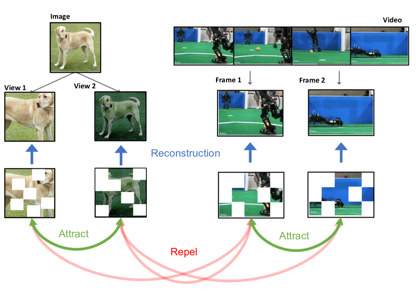
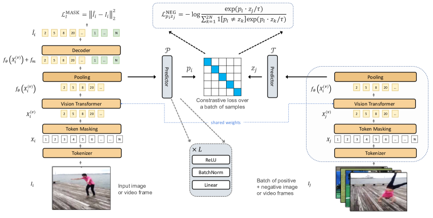
Building on masked image modeling and image-level similarity learning, we propose to learn representations by using masking image modeling at the image level, and image-level similarity either using sample frames or augmented images. This means that each video frame is pulled towards a global video representation in the latent space. This can lead to representations that are invariant to object deformations, appearance changes and viewpoint variations. See Figure 2 for a general overview of our model. The pseudocode of ViC-MAE is also provided in Algortihm 1.

Given a video with $T$ frames $\{I_{1},I_{2},\cdots,I_{T}\}$, we sample two frames $I_{i},I_{j}$ as a positive pair input during one step of training. We treat single images as videos with $T=1$ and augment them when this is the case. After an input image tokenizer layer we obtain a set of patch-level token representations $X_{i}$ and $X_{j}$ for each frame. Then, we apply token masking by generating a different random mask $M_{i}$ and $M_{j}$ and apply them to both of the corresponding input frames to obtain a subset of input visible tokens $X_{i}^{(v)}$ and $X_{j}^{(v)}$. These visible token sets are then forwarded to a ViT encoder which computes a set of representations $f_{\theta}(X_{i}^{(v)})$ and $f_{\theta}(X_{j}^{(v)})$ respectively. Finally, for the first image we compute $\hat{I}_{i}=d_{\phi}(f_{\theta}(X_{i}^{(v)}+f_{m}))$ where we have added a mask token $f_{m}$ to let the decoder know which patches were masked and allows to predict patch-shaped outputs through $\hat{I}_{i}$. These output patches are then trained to minimize the $\ell_{2}$ loss with the true patches in the input image:

$$\mathcal{L}_{i}^{\text{MASK}}=\lVert\hat{I}_{i}-I_{i}\rVert_{2}^{2}.$$ (2)

So far we have described only a standard masked autoencoder (MAE). In order to apply contrastive pre-training we use a separate prediction branch in the network by applying a global pooling operator $\Omega$ over the output representations $f_{\theta}(X_{i}^{(v)})$ from the main branch and $f_{\theta}(X_{j}^{(v)})$ from the siamese copy of the network. This step simplifies the formulation of our method and avoids using additional losses or the gradient-stop operator as in SimSiam [13] to avoid feature representation collapse since the pooled features can not default to the zero vector as they also are being trained to reconstruct patches. We experiment using various aggregation methods including mean pooling, max pooling, and generalized mean (GeM) pooling [65]. These global representations are then forwarded to a predictor encoder $\mathcal{P}$ and a target encoder $\mathcal{T}$ to obtain frame representations:

$$p_{i}\triangleq\mathcal{P}(\Omega(f_{\theta}(X_{i}^{(v)})))/\lVert\mathcal{P}(\Omega(f_{\theta}(X_{i}^{(v)}))))\rVert_{2},$$

and

$$z_{j}\triangleq\mathcal{T}(\Omega(f_{\theta}(X_{j}^{(v)})))/\lVert\mathcal{T}(\Omega(f_{\theta}(X_{j}^{(v)}))))\rVert_{2}$$

respectively. The predictor network $\mathcal{P}$ and target network $\mathcal{T}$ are symmetrical and we use standard blocks designed for contrastive learning [5, 11, 13]. These blocks consist of a Linear $\rightarrow$ BatchNorm1d $\rightarrow$ ReLU block repeated $2$ times. From these representations, we apply the InfoNCE contrastive learning loss as follows:

$$\mathcal{L}^{\text{NEG}}_{p_{i},z_{j}}=-\log\frac{\text{exp}(p_{i}\cdot z_{j}/\tau)}{\sum^{2N}_{k=1}\mathbbm{1}[p_{i}\neq z_{k}]\text{exp}(p_{i}\cdot z_{k}/\tau)},$$ (3)

where the denominator includes a set of negative pairs with representations $z_{k}$ computed for frames from other videos in the same batch, $\mathbbm{1}[p_{i}\neq z_{k}]\in\{0,1\}$ is an indicator function evaluating to $1$ when $p_{I}\neq z_{k}$ and $\tau$ denotes a temperature parameter.

The final loss is $\mathcal{L}=\mathcal{L}^{\text{MASK}}+\lambda\mathcal{L}^{\text{NEG}}$, where $\lambda$ is a hyperpameter controlling the relative influence of both losses. In practice, we use an schedule to gradually introduce the contrastive loss and let the model learn good local features at the beginning of training.

4 Experiment Settings

	Method	Arch.	Pre-training Data	In-Domain			Out-of-Domain
				IN1K	K400		Places-365	SSv2
Supervised	ViT [22] ICML’20	ViT-B	IN1K	82.3	68.5		57.0	61.8
	ViT [22] ICML’20	ViT-L	IN1K	82.6	78.6		58.9	66.2
	OMNIVORE [27] CVPR’22	ViT-B	IN1K + K400 + SUN RGB-D	84.0	83.3		59.2	68.3
	OMNIVORE [27] CVPR’22	ViT-L	IN1K + K400 + SUN RGB-D	86.0	84.1		–	–
	TubeViT [63] CVPR’23	ViT-B	K400 + IN1K	81.4	88.6		–	–
	TubeViT [63] CVPR’23	ViT-L	K400 + IN1K	–	90.2		–	76.1
Self-Supervised	MAE [35] CVPR’22	ViT-B	IN1K	83.4	–		57.9	59.6
	MAE [35] CVPR’22	ViT-L	IN1K	85.5	82.3		59.4	57.7
	ST-MAE [26] NeurIPS’22	ViT-B	K400	81.3	81.3		57.4	69.3
	ST-MAE [26] NeurIPS’22	ViT-L	K400	81.7	84.8		58.1	73.2
	VideoMAE [68] NeurIPS’22	ViT-B	K400	81.1	80.0		–	69.6
	VideoMAE [68] NeurIPS’22	ViT-L	K400	–	85.2		–	74.3
	OmniMAE [29] CVPR’23	ViT-B	K400 + IN1K	82.8	80.8		58.5	69.0
	OmniMAE [29] CVPR’23	ViT-L	K400 + IN1K	84.7	84.0		59.4	73.4
	ViC-MAE	ViT-L	K400	85.0	85.1		59.5	73.7
	ViC-MAE	ViT-L	MiT	85.3	84.9		59.7	73.8
	ViC-MAE	ViT-B	K400 + IN1K	83.0	80.8		58.6	69.5
	ViC-MAE	ViT-L	K400 + IN1K	86.0	86.8		60.0	75.0
	ViC-MAE	ViT-B	K400 + K600 + K700 + MiT + IN1K	83.8	80.9		59.1	69.8
	ViC-MAE	ViT-L	K400 + K600 + K700 + MiT + IN1K	87.1	87.8		60.7	75.9

Table 1: Transfer learning results from video and image pre-training to various datasets using the ViT/L-16 backbone. The pre-training data is a video dataset (MiT, K600 or K400) and/or image dataset (IN1K). All self-supervised method are evaluated end-to-end with supervised finetuning on IN1K, Kinetics-400, Places365, and SSv2. Best results are in bold. Results of MAE, ST-MAE and VideoMAE for out of domain data were taken from Girdhar et al. [29].

We perform experiments to demonstrate the fine-tuning performance of our method on ImageNet-1k, and other image recognition datasets. We also evaluate our method on the Kinetics dataset [38] and Something Something-v2 [33] for action recognition to show that our model is able to maintain performance on video benchmarks. Full details are in the appendix.

Architecture. We use the standard Vision Transformer (ViT) architecture [22] and conduct experiments fairly across benchmarks and methods using the ViT-B/16 and ViT-L/16 configurations. For masked image modeling we use a small decoder as proposed by He et al. [35].

Pre-Training. We adopt Moments in Time [56], Kinetics-400  [38] and ImageNet-1k [20] as our main datasets for self supervised pre-training. They consist on $\sim$1000K and $\sim$300K videos of varied length respectively, and $\sim$1.2M images for Imagenet-1k. We sample frames from these videos using distant sampling, which consists of splitting the video in non-overlapping sections and sampling one frame from each section. Frames are resized to a 224 pixel size, horizontal flipping and random cropping with a scale range of $[0.5,1]$, as the only data augmentation transformations on video data. Random cropping (with flip and resize), color distortions, and Gaussian blurring are used for the image modality.

Settings. ViC-MAE pre-training follows previously used configurations [35, 26]. We use the AdamW optimizer with a batch size of 512 per device. We evaluate the pre-training quality by end-to-end finetuning. When evaluating on video datasets we follow the common practice of multi-view testing: taking $K$ temporal clips ($K=7$ on Kinetics) and for each clip taking 3 spatial views to cover the spatial axis (this is denoted as $K\times 3$). The final prediction is the average of all views.

5 Results and Ablations

We first perform experiments to analyze the different elements of the ViC-MAE framework. All the experiments are under the learning with negative pairs setting using mean pooling over the ViT features. Linear evaluation and end-to-end finetuning runs are done over 100 epochs for ImageNet-1k, see appendix for more details. For our ablations, we restrict ourselves to the ViT-B/16 architecture pre-trained over 400 epochs unless specified otherwise.

5.1 Main result

Model	Pre-train.	Food	CIFAR10	CIFAR100	Birdsnap	SUN397	Cars	Aircraft	VOC2007	DTD	Pets	Caltech101	Flowers
MAE [35] ‡	K400	74.54	94.86	79.49	46.51	64.33	60.10	63.24	83.07	78.01	89.49	93.28	93.38
MAE [35] ‡	MiT	76.23	94.47	79.50	47.98	65.32	59.48	60.67	83.46	78.21	88.42	93.08	94.17
ViC-MAE (ours)	K400	76.56	93.64	78.80	47.56	64.75	58.96	60.14	83.74	78.53	87.65	92.27	93.35
ViC-MAE (ours)	MiT	77.39	94.92	79.88	48.21	65.64	59.76	60.96	84.77	79.27	88.85	93.53	94.62

Table 2: Comparison of transfer learning performance of our approach with supervised baselines across 12 natural image classification datasets. All results correspond to linear evaluation. Best results are shown in bold. ‡MAE trained on MiT and K400 randomly sample a frame from the video to compute a reconstruction loss; these models are trained and evaluated by us.

Our main result evaluates ViC-MAE on two in-domain datasets that were used during training for most experiments: ImageNet-1K (images) and Kinetics-400 (video), and two out-of-domain datasets that no methods used during training: Places-365 [82] (images) and Something-something-v2 (video). Table 1 shows our complete set of results including comparisons with the state-of-the-art on both supervised representation learning (typically using classification losses), and self-supervised representation learning (mostly using masked image modeling). We consider mostly recent methods building on visual transformers as the most recent TubeViT [63] which is the state-of-the-art on these benchmarks relies on this type of architecture.

Our most advanced version of ViC-MAE trained on five datasets (Kinetics-400, Kinetics-600, Kinetics-700, Moments in Time and Imagenet-1k) using the ViT-Large architecture performs the best across all metrics on all datasets compared to all previous self-supervised representation learning methods and even outperforms the supervised base model OMNIVORE [27] on Imagenet-1k with a top-1 accuracy of 87.1% vs 86%. ViC-MAE also comes a close second to other supervised methods and roughly matches the performance of TubeViT [63] which obtains 76.1% top-1 accuracy on Something something-v2 compared to our 75.9% top-1 accuracy. When compared to the current self-supervised state-of-the-art OmniMAE using the same ViT-Large architecture and the same datasets for pre-training (Kinetics-400 and Imagenet-1k), ViC-MAE also outperforms OmniMAE in all benchmarks (Imagenet: 86% vs. 84.7%, Kinetics-400: 86.8% vs. 84%, Places-365: 60% vs. 59.4% and SSv2: 75% vs 73.4%).

Another important result is video-to-image transfer which is the setting where the model is only trained on video but its performance is tested on downstream image tasks. Table 1 shows that when ViC-MAE is trained on the Moments in Time dataset [56], it achieves the best top-1 accuracy of 85.3% for any self-supervised backbone model trained only on video. These results highlight the closing gap in building robust representations that can work seamlessly across image and video tasks.

5.2 Comparison with other contrastive masked autoencoders.

Combining MAE with joint-embedding methods is non trivial. In our first attempts, we used the [CLS] token as the representation and apply negative free methods such as VicReg [5], and SimSiam [13] with limited success (See appendix). When combined with contrastive methods, we found best to use a pooling operation over the ViT features similar to CAN [55], as we find worse performance when the [CLS] token is used, like in C-MAE [37]. The original MAE [35] is known to have poor linear evaluation performance obtaining 68% in IN1K linear evaluation when pre-trained on IN1K [35, 42]. On the contrary, SimCLR [12] a model trained only using contrastive learning on IN1K achieves 73.5%. Several works have tried to address this by combining contrastive learning with masked image modelling to get the best of both worlds. CAN [55], C-MAE [37] and MAE-CT [42] obtain linear evaluation accuracies of 74.0%, 73.9, 73.4%, respectively when trained on IN1K while ViC-MAE obtains 74.0% trained only on IN1K using ViT/B-16 pre-trained for 800 epochs to make the comparison fair. When using the K400 and IN1K datasets together for pre-training, we get 73.6%, but we highlight that ViC-MAE is now able to maintain good performance in videos and images using the same pre-trained model.

Frame separation	ImageNet-1K
	Top-1	Top-5
0	63.25	83.34
2	64.47	84.31
4	65.25	84.64
8	65.89	84.91
D	67.66	86.22

Table 3: Ablation on frame separation. Linear evaluation on the ImageNet-1K dataset using different frame separartion. 0 means sample the same frame. D stands for distant sampling and the rest are using continuos sampling.

5.3 Video-to-image transfer learning performance.

We evaluate transfer learning performance of ViC-MAE across a diverse array of 12 downstream image classification tasks [8, 40, 6, 78, 39, 53, 16, 60, 24, 57]. Table 2 shows the results of four models based on a ViT/B backbone. We perform linear evaluation (See appendix for details on the metrics used to evaluate each of these models). We train two models using two video datasets. The first model is a baseline MAE model pre-trained on randomly sampled frames from videos on the Moments in Time dataset and the Kinetics-400 dataset. The second model is our full ViC-MAE model pre-trained on each of the same two datasets. Our model significantly outperforms the other baselines on 9 out of 12 datasets, whereas the MAE trained on Kinetics is superior on only 3 (i.e. Cars, Aircraft and Pets).

5.4 Ablations

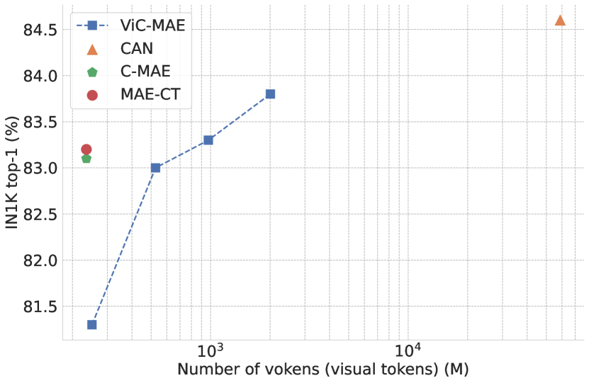
We investigate the effect of scaling the data used to train ViC-MAE, the effect of the ratio of image to videos in pre-training, the effect of our choice of frame separation, and the choice of pooling operator. Influence of pre-training data. We perform an ablation study to the effect of scaling the data points seen by the model. The pre-training data includes Kinectis-400, ImageNet-1K, Kinectis-600 + Kinectis-700, and the Moments in Time datasets added in that order. We pre-train a ViT/B-16 using ViC-MAE for 400 epochs. As illustrated in Figure 3, as we progressively increase the dataset size, our ViC-MAE, shows a steady increase in IN1K top-1 accuracy. This is remarkably, when compared to CAN [55], pre-trained on the JFT-300M dataset for 800 epochs that only reaches an accuracy of 84.4%. This shows that our model, when supplied with only about 1.5% of the data that CAN was trained on (4.25M vs. 300M), can achieve comparable accuracy levels.

Model	Pooling type	ImageNet-1K
		Top-1	Top-5
ViC-MAE (Ours)	GeM	66.92	85.50
ViC-MAE (Ours)	max	67.01	85.59
ViC-MAE (Ours)	mean	67.66	86.22

Table 4: Ablation on pooling type. Linear evaluation on the ImageNet-1K dataset using different types of pooling. The hyperparmeter $\lambda$ is set to $0.025$ and introduced using an schedule.

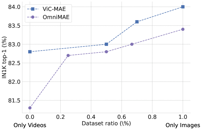
Contrastive vs Masking-only pre-training We perform an ablation study to the effect varying the ratio of images to video in the dataset by replicating the entire datasets, notice that the number of training updates change when doing this. The pre-training data includes Kinectis-400 and ImageNet-1K. We pre-train a ViT/B-16 using ViC-MAE for 400 epochs. As illustrated in Figure 4, as we progressively increase the ratio of images to videos, our ViC-MAE, surpases the OmniMAE model [79], meaning that contrastive plus masking pre-training is better able to use image and video data than masking-only pre-training.

Frame separation. This is an essential design of our framework, and in this experiment we aim to see the effect of frame separation on model performance. We follow the two methods of sampling frames from Xu et.al [79]. Results are shown in Table 3. The first method is Continuous sampling which consists in selecting a starting index $i$ and then sampling a frame in the interval $(i,i+\delta]$, where $\delta$ is the frame separation. A frame separation of $0$ indicates that the predictor and the target networks receive the same frame. The second method is distant sampling, where the video is split into $n$ intervals of the same size, where $n$ is the number of frames to use for contrastive learning and then one frame is selected randomly from each interval. In our experiment, we observe that increasing the frame separation when using continuous sampling increases model performance. We observe the best performance using distant sampling with $n=2$ (labelled $D$ in Table 3). We posit that further increasing frame separation offers potentially stronger augmentations. In the following experiments, we only use strong spatial augmentations combined with distant frame sampling.

Figure 3: ViC-MAE using the ViT/B-16 architecture finetuned on IN1K for 100 epochs, compared with CAN [55] pre-trained on JFT-300M, C-MAE [37], and MAE-CT [42] pre-trained on ImageNet-1K. We increase the amount of data points by adding more video datasets. We can see that our model reaches similar accuracy with $\approx 4.25$M data points compared to the $300$M of the JFT-300M dataset.

Pooling type. Since this is an important step in our proposed method, we test which operator $\Omega$ used to aggregate local features performs best at producing global features. We report our results in Table 4. We try common types of pooling (mean, max) as well as, generalized mean pooling. We found mean to be more effective in creating a global representation for the video, and we use it for all other experiments.

5.5 Limitations

Having shown that ViC-MAE is able to learn useful representations from video and image data that transfer well to video and image classification and that surpasses previous models on the same set-up, we contextualize our results by discussing state of the art results in these problems and limitations of our method.

Within similar computational constraints, ViC-MAE matches prior results on Kinetics-400, trailing supervised models like TubeViT [63] by $7.1\%$ on ViT/B-16 and $2.4\%$ on ViT/L-16, and MVT [80] slightly on ViT/B-16 but surpasses it by $3.5\%$ on ViT/L-16. It also exceeds MViTv1 [23], TimeSformer [7], and ViViT [2] by margins up to $7.3\%$ on ViT/L-16. Compared to self-supervised models, ViC-MAE falls behind MaskFeat [76] by $0.7\%$ on ViT/B-16 but excels on ViT/L-16 by $3.5\%$. It is slightly outperformed by DINO [9] and more substantially by models utilizing extra text data or larger image datasets, such as UMT [44], MVD [73], and UniFormerV2 [43], by up to $4.2\%$ on ViT/B-16 and $2.8\%$ on ViT/L-16.

When compared against state-of-the-art ImageNet-pretrained models with comparable computational resources, video-based models, including ours, typically fall short. However, including image and video modalities shows promise in boosting performance. Against models using masked image modeling and contrastive learning, ViC-MAE modestly surpasses MAE [35] by $1.6\%$ and MaskFeat [76] by $1.4\%$ with the ViT/L-16 architecture. It also edges out MoCov3 [14] and BeiT [4] by $3\%$ and $1.9\%$ respectively on the same architecture. Yet, it lags behind DINOv2 [59] by $1.2\%$ for ViT/L-16. When compared to supervised models using additional image data, such as DeiT-III [69] and SwinV2 [47] and the distilled ViTs’ from [19], our model shows a lag behind of $0.8\%$, $1.2\%$ and $2.5\%$ respectively on ViT/L-16. These results show that the gap from models pre-trained purely on video still exists but we believe ViC-MAE pre-trained on image and video data is a step forward in closing that gap.

Figure 4: ViC-MAE using the ViT/B-16 architecture finetuned on IN1K for 100 epochs, compared with OmniMAE[29]. We vary the ratio of images vs video in the dataset, from no images to only images. We can see that our ViC-MAE can better utilize the videos and images on the dataset than masking-only pre-training.

6 Conclusion

In this work, we introduce ViC-MAE, a method that allows to use unlabeled videos and images to learn useful representation for image recognition tasks. We achieve this by randomly sampling frames from a video or creating two augmented views of an image and using contrastive learning to pull together inputs from the same video and push apart inputs from different videos, likewise we also use masked image modeling on each input to learn good local features of the scene presented in each input. The main contribution of our work is showing that is possible to combine masked image modeling and contrastive learning by pooling the local representations of the MAE prediction heads into a global representation that is used for contrastive learning. The design choices that we have taken, when designing ViC-MAE show that our work is easily extensible in various different ways. For example, improvements in contrastive learning for images can be directly adapted into our framework. Likewise, pixel reconstruction can be replaced by features that are important for video representation such as object correspondences or optical flow.

Appendix A Implementation Details

We will release code and model checkpoints, along with the specific training configurations. We followed previous training configurations that also worked well for our models [35, 26].

ViC-MAE architecture.

We follow the standard ViT architecture [22], which has a stack of Transformer blocks, each of which consists of a multi-head attention block and an Multi-Layer Perceptron (MLP) block, with Layer Normalization (LN). A linear projection layer is used after the encoder to match the width of the decoder. We use sine-cosine position embeddings for both the encoder and decoder. For the projection and target networks, we do average pooling on the encoder features and follow the architecture of Bardes et al. [5], which consists of a linear layer projecting the features up to twice the size of the encoder and two blocks of linear layers that preserve the size of the features, followed by batch normalization and a ReLU non-linearity.

We extract features from the encoder output for fine-tuning and linear probing. We use the class token from the original ViT architecture, but notice that similar results are obtained without it (using average pooling).

Video Loading.

In order to prevent video loading from being a bottleneck on performance due to time spent on video decoding, we leverage the ffcv library [41], which we modify to support videos as a list of images in the WebP format. This allows us to significantly surpass the default PyTorch data loaders which can only read data in a synchronous fashion, resulting in the process being blocked until video decoding is complete. The use of ffcv allows to perform training without the need of sample repetition as done in OmniMAE [29] and ST-MAE [26] at the cost of a significantly larger storage requirement. We will also release the code for ffcv to support videos.

Pre-training.

The default settings can be found in Table 5. We do not perform any color augmentation, path dropping or gradient clipping. We initialize our transformer layer using xavier_uniform [30], as it is standard for Transformer architectures. We use the linear learning rate (lr) scaling rule so that lr = base_lr$\times$batchsize / 256 [32].

End-to-end finetuning.

We follow common practice for end-to-end finetuning. Default settings can be found in Table 6. Similar to previous work, we use layer-wise lr decay [35].

Linear evaluation.

We follow previous work for linear evaluation results [35, 26]. As previous work has found we do not use common regularization techniques such as mixup, cutmix, and drop path, and likewise, we set the weight decay to zero [15]. We add an extra batch normalization layer without the affine transformation after the encoder features. Default settings can be found in Table 7.

config	value
optimizer	AdamW [50]
base learning rate	1.5e-4
weight decay	0.05
optimizer momentum	$\beta_{1},\beta_{2}{=}0.9,0.95$ [10]
batch size	4096
learning rate schedule	cosine decay [49]
warmup epochs [32]	40
epochs	800
augmentation	hflip, crop [0.5, 1]
contrastive loss weight $\lambda$	0.025
contrastive loss schedule	0 until epoch 200 then 0.025

Table 5: Pre-training setting.

config	ViT/B	ViT/L
optimizer	AdamW
optimizer momentum	$\beta_{1},\beta_{2}{=}0.9,0.999$
base learning rate
IN1K	3e-3	0.5e-3
P65	2e-3
K400	1.6e-3	4.8e-3
SSv2	1e-3
weight decay	0.05
learning rate schedule	cosine decay
warmup epochs	5
layer-wise lr decay [17, 4]	0.65	0.75
batch size	1024	768
training epochs
IN1K	100	50
P65	60	50
K400	150	100
SSv2	40
augmentation	RandAug (9, 0.5) [18]
label smoothing [67]	0.1
mixup [81]	0.8
drop path [36]	0.1	0.2

Table 6: End-to-end fine-tuning setting.

config	value
optimizer	SGD
base learning rate	0.1
weight decay	0
optimizer momentum	0.9
batch size	4096
learning rate schedule	cosine decay
warmup epochs	10
training epochs	90
augmentation	RandomResizedCrop

Table 7: Linear evaluation setting.

Appendix B What we tried and did not work:

Method	ImageNet-1K
	Top-1	Top-5
MAE [35] + SiamSiam [13]	58.58	82.88
MAE [35] + VicReg [5]	63.86	84.07
ViC-MAE (ours)	67.66	86.22

Table 8: Combining MAE and contrastive methods is not trivial. Linear evaluation on the ImageNet-1K dataset using types of contrastive learning. We use the $[\text{CLS}]$ token as the global video representation and apply common contrastive methods, but these do not result on the best performance, which is obtained with our method.

B.1 Combining MAE with Negative-Free Methods.

We tried to combine MAE with instance discrimination learning methods by using the $[\text{CLS}]$ token of the transformer as a global video feature representation. This representation allows us to use any instance discrimination learning loss without modifications to the underlying ViT transformer encoder. This combination works as follows: Sample two images from a video or an image and its transformed version $I_{i},I_{j}$ and perform patch-level masking. The two inputs are processed by the ViT model $f_{\theta}$ producing token representations $f_{\theta}(I_{i})=\{x_{i}^{\text{CLS}},x_{i}^{1},x_{i}^{2},\cdots,x_{i}^{L}\}$, where $L$ is the sequence length of the transformer model. This is divided into two disjoint sets. The set $\{x_{i}^{1},x_{i}^{2},\cdots,x_{i}^{L}\}$ represents the local features of the input $i$ and are used for masked image modeling following Eq. 1. Then, the $x_{i}^{\text{CLS}}$ token can be used as a global representation with a contrastive loss.

We experiment with this approach using the SimSiam loss [13] and the VicReg loss [5]. We review here these methods and how to combine them with MAEs, but the reader is referred to the original works for a more in-depth explanation of these methods [13, 5].

SimSiam.

A combination of SimSiam and MAE, which we refer to as MAE + SimSiam uses the $x_{i}^{\text{CLS}}$ token which represents the global video representation as follows: We pass $x_{i}^{\text{CLS}}$ to a projector network $\mathcal{P}$ to obtain $p_{i}\triangleq\mathcal{P}(x_{i}^{\text{CLS}})/\lVert\mathcal{P}(x_{i}^{\text{CLS}})\rVert_{2}$. A similar procedure is followed for input $j$, but the global representation is not passed to the projector network $\mathcal{P}$ in order to obtain $z_{j}\triangleq x_{i}^{\text{CLS}}/\lVert x_{i}^{\text{CLS}}\rVert_{2}$. The SimSiam objective is then applied as follows:

$$\mathcal{L}^{\text{ \tiny SimSiam}}_{p_{i},z_{j}}=\lVert p_{i}-z_{j}\rVert^{2}_{2}=2(1-p_{i}\cdot z_{j}).$$ (4)

VicReg.

A combination of VicReg and MAE, which we refer to as MAE + VicReg uses the $x_{i}^{\text{CLS}}$ token which represents the global video representation as follows: We pass it to a projector network $\mathcal{P}$ to obtain $p_{i}\triangleq\mathcal{P}(x_{i}^{\text{CLS}})/\lVert\mathcal{P}(x_{i}^{\text{CLS}})\rVert_{2}$, we repeat this procedure for input $j$ using the target network $\mathcal{T}$ to obtain $z_{i}\triangleq\mathcal{T}(x_{i}^{\text{CLS}})/\lVert\mathcal{T}(x_{i}^{\text{CLS}})\rVert_{2}$. The loss is calculated at the embedding level on $p_{i}$ and $z_{j}$. The inputs are processed in batches, let us denote $P=[p^{1},\cdots,p^{n}]$ and $Z=[z^{1},\cdots,z^{n}]$, where each $p^{m}$ and $z^{m}$ are the global representation of video $m$ after the projector network and target network respectively in a batch of size $n$ vectors of dimension $d$. Let us denote by $p_{l}$ the vector composed of each value at dimension $l$ in all vectors in $P$. The variance loss of VicReg is then calculated as follows:

$$v(P)=\frac{1}{d}\sum_{l=1}^{d}\text{max}(0,\gamma-S(p_{i},\epsilon)),$$ (5)

where $S(z,\epsilon)=\sqrt{\text{Var}(z)+\epsilon}$ and $\gamma$ is a constant target value for the standard deviation, fixed to 1. The covariance loss of VicReg can be calculated as:

$$c(P)=\frac{1}{d}\sum_{l\neq k}^{d}[\text{Cov}(p^{m})]^{2}_{l,k},$$ (6)

where $\text{Cov}(p^{m})=\frac{1}{N-1}\sum_{m}(p^{m}-\bar{p})(p^{m}-\bar{p})^{T}$. The final VicReg loss over the batch is defined as:

$$\mathcal{L}^{\text{\tiny VicReg}}_{p_{i},z_{j}} =\frac{\lambda}{n}\lVert p_{i}-z_{j}\rVert^{2}_{2}+\mu\left[v(P)+v(Z)\right]+\nu\left[c(P)+c(Z)\right].$$ (7)

Percentage of data	5%	10%	25%	50%	75%	100%
MAE [35] + SimSiam [13]	7.15	23.41	39.73	54.94	62.88	67.44
MAE [35] + VicReg [5]	47.48	56.63	66.62	73.00	75.29	77.41
ViC-MAE (ours)	50.25	58.22	67.65	73.97	75.80	77.89

Table 9: Semi-supervised evaluation on ImageNet. We performed end-to-end finetuning using the settings in 6, but disable RandAug and MixUp for this experiment.

We perform experiments using these two combinations of MAE and contrastive losses as baseline comparisons for our method but found them to be underperforming with only contrastive or only masked methods. In other words, it is not trivial to adapt constrastive learning methods to be used in combination with masked autoencoders. See Table 8 for more details. For the contrastive learning part we experiment with two alternatives.

• MAE + {SimSiam or VicReg}. The predictor consists of the backbone network $f_{\theta}$ and a projector followed by a predictor as in Bardes et al. [5]. The target encoder consists of the backbone $f_{\theta}$ and the projector, which are shared between the two encoders.

• ViC-MAE. The predictor and the target networks share the same architecture consisting of the backbone network $f_{\theta}$ and a projector following Bardes et al. [5].

When using the MAE + {SimSiam or VicReg} combinations, we use the $[\text{CLS}]$ token from the ViT architecture which is typically used to capture a global feature from the transformer network and is used to fine-tune the network for downstream tasks such as classification.

Combining MAE with negative-free representation learning is non trivial, and we set to test these by comparing our model with MAE models with alternative negative-free learning objectives Siamsiam [13] and VicReg [5]. We present our results using linear evaluation on Table 8. We use the $[\text{CLS}]$ token as the global video representation for contrastive pre-training for 400 epochs. We can notice that competing methods underperform compared to our model which uses pooling of the local features by an absolute margin of $>3\%$ over the MAE + VicReg model.

Semi-supervised evaluation on ImageNet.

We also test ViC-MAE against negative-free representation learning methods on the problem of Semi-Supervised evaluation on the ImageNet dataset. The setting consists on training on a subset of the training data and testing on the whole validation data. We chose subsets of size 5%, 10%, 25%, 50%, 75% and 100% of the whole training set of ImageNet. We compare our model against MAE [35] + SimSiam [13], and MAE [35] + VicReg [5]. Results are shown on Table 9, and show the supperiority of ViC-MAE over simple combinations of contrastive learning and masked image modeling.

Color Augm.	Spatial Augm.	ImageNet-1K
		Top-1	Top-5
		65.40	84.03
		66.03	85.01
		67.66	86.22

Table 10: Ablation on different augmentations. Linear evaluation on the ImageNet-1K dataset using different augmentations. Color augs include random color jitter, grayscale conversion and gaussian blur. Spatial augs are random resized crop and horizontal flip.

B.2 Adding strong augmentations to the video frames

We perform an ablation study to check whether the use of strong color augmentations on the target encoder is necessary for the video frames as it is for the images when we train simultaneously. The results are presented in Table 10. Using only color augmentations meaning that the sampled frame in the target encoder is color augmented but not spatially augmented the performance is reduced by $>2\%$ on linear evaluation on the Imagenet dataset. Using a combination of strong color augmentations and spatial augmentations, though it increases performance; it is not superior to using only strong spatial augmentations. This is stark contrast with previous methods that necessitate strong color augmentations to be able to learn using contrastive learning. This might suggest the the natural augmentation from time shift is enough when using video frames and making it harder by imposing strong color augmentations just diminishes performance. Notice that when using images from an image dataset, we still use strong color and spatial augmentations.

References

- Agrawal et al. [2015] Pulkit Agrawal, Joao Carreira, and Jitendra Malik. Learning to see by moving. In Proceedings of the IEEE international conference on computer vision, pages 37–45, 2015.
- Arnab et al. [2021] Anurag Arnab, Mostafa Dehghani, Georg Heigold, Chen Sun, Mario Lučić, and Cordelia Schmid. Vivit: A video vision transformer. In Proceedings of the IEEE/CVF international conference on computer vision, pages 6836–6846, 2021.
- Assran et al. [2022] Mahmoud Assran, Mathilde Caron, Ishan Misra, Piotr Bojanowski, Florian Bordes, Pascal Vincent, Armand Joulin, Mike Rabbat, and Nicolas Ballas. Masked siamese networks for label-efficient learning. In European Conference on Computer Vision, pages 456–473. Springer, 2022.
- Bao et al. [2021] Hangbo Bao, Li Dong, Songhao Piao, and Furu Wei. Beit: Bert pre-training of image transformers. In International Conference on Learning Representations, 2021.
- Bardes et al. [2022] Adrien Bardes, Jean Ponce, and Yann Lecun. Vicreg: Variance-invariance-covariance regularization for self-supervised learning. In ICLR 2022-International Conference on Learning Representations, 2022.
- Berg et al. [2014] Thomas Berg, Jiongxin Liu, Seung Woo Lee, Michelle L Alexander, David W Jacobs, and Peter N Belhumeur. Birdsnap: Large-scale fine-grained visual categorization of birds. In Proceedings of the IEEE Conference on Computer Vision and Pattern Recognition, pages 2011–2018, 2014.
- Bertasius et al. [2021] Gedas Bertasius, Heng Wang, and Lorenzo Torresani. Is space-time attention all you need for video understanding? In International Conference on Machine Learning, pages 813–824. PMLR, 2021.
- Bossard et al. [2014] Lukas Bossard, Matthieu Guillaumin, and Luc Van Gool. Food-101–mining discriminative components with random forests. In Computer Vision–ECCV 2014: 13th European Conference, Zurich, Switzerland, September 6-12, 2014, Proceedings, Part VI 13, pages 446–461. Springer, 2014.
- Caron et al. [2021] Mathilde Caron, Hugo Touvron, Ishan Misra, Hervé Jégou, Julien Mairal, Piotr Bojanowski, and Armand Joulin. Emerging properties in self-supervised vision transformers. In Proceedings of the IEEE/CVF International Conference on Computer Vision, pages 9650–9660, 2021.
- Chen et al. [2020a] Mark Chen, Alec Radford, Rewon Child, Jeffrey Wu, Heewoo Jun, David Luan, and Ilya Sutskever. Generative pretraining from pixels. In International conference on machine learning, pages 1691–1703. PMLR, 2020a.
- Chen et al. [2020b] Ting Chen, Simon Kornblith, Mohammad Norouzi, and Geoffrey Hinton. A simple framework for contrastive learning of visual representations. In International conference on machine learning, pages 1597–1607. PMLR, 2020b.
- Chen et al. [2020c] Ting Chen, Simon Kornblith, Kevin Swersky, Mohammad Norouzi, and Geoffrey E Hinton. Big self-supervised models are strong semi-supervised learners. Advances in neural information processing systems, 33:22243–22255, 2020c.
- Chen and He [2021] Xinlei Chen and Kaiming He. Exploring simple siamese representation learning. In Proceedings of the IEEE/CVF Conference on Computer Vision and Pattern Recognition, pages 15750–15758, 2021.
- Chen et al. [2020d] Xinlei Chen, Haoqi Fan, Ross Girshick, and Kaiming He. Improved baselines with momentum contrastive learning. arXiv preprint arXiv:2003.04297, 2020d.
- Chen et al. [2021] Xinlei Chen, Saining Xie, and Kaiming He. An empirical study of training self-supervised vision transformers. In Proceedings of the IEEE/CVF International Conference on Computer Vision, pages 9640–9649, 2021.
- Cimpoi et al. [2014] Mircea Cimpoi, Subhransu Maji, Iasonas Kokkinos, Sammy Mohamed, and Andrea Vedaldi. Describing textures in the wild. In Proceedings of the IEEE conference on computer vision and pattern recognition, pages 3606–3613, 2014.
- Clark et al. [2019] Kevin Clark, Minh-Thang Luong, Quoc V Le, and Christopher D Manning. Electra: Pre-training text encoders as discriminators rather than generators. In International Conference on Learning Representations, 2019.
- Cubuk et al. [2020] Ekin D Cubuk, Barret Zoph, Jonathon Shlens, and Quoc V Le. Randaugment: Practical automated data augmentation with a reduced search space. In Proceedings of the IEEE/CVF conference on computer vision and pattern recognition workshops, pages 702–703, 2020.
- Dehghani et al. [2023] Mostafa Dehghani, Josip Djolonga, Basil Mustafa, Piotr Padlewski, Jonathan Heek, Justin Gilmer, Andreas Peter Steiner, Mathilde Caron, Robert Geirhos, Ibrahim Alabdulmohsin, et al. Scaling vision transformers to 22 billion parameters. In International Conference on Machine Learning, pages 7480–7512. PMLR, 2023.
- Deng et al. [2009] Jia Deng, Wei Dong, Richard Socher, Li-Jia Li, Kai Li, and Li Fei-Fei. Imagenet: A large-scale hierarchical image database. In 2009 IEEE conference on computer vision and pattern recognition, pages 248–255. Ieee, 2009.
- Diba et al. [2019] Ali Diba, Vivek Sharma, Luc Van Gool, and Rainer Stiefelhagen. Dynamonet: Dynamic action and motion network. In Proceedings of the IEEE/CVF International Conference on Computer Vision, pages 6192–6201, 2019.
- Dosovitskiy et al. [2020] Alexey Dosovitskiy, Lucas Beyer, Alexander Kolesnikov, Dirk Weissenborn, Xiaohua Zhai, Thomas Unterthiner, Mostafa Dehghani, Matthias Minderer, Georg Heigold, Sylvain Gelly, et al. An image is worth 16x16 words: Transformers for image recognition at scale. In International Conference on Learning Representations, 2020.
- Fan et al. [2021] Haoqi Fan, Bo Xiong, Karttikeya Mangalam, Yanghao Li, Zhicheng Yan, Jitendra Malik, and Christoph Feichtenhofer. Multiscale vision transformers. In Proceedings of the IEEE/CVF International Conference on Computer Vision, pages 6824–6835, 2021.
- Fei-Fei et al. [2004] Li Fei-Fei, Rob Fergus, and Pietro Perona. Learning generative visual models from few training examples: An incremental bayesian approach tested on 101 object categories. In 2004 conference on computer vision and pattern recognition workshop, pages 178–178. IEEE, 2004.
- Feichtenhofer et al. [2021] Christoph Feichtenhofer, Haoqi Fan, Bo Xiong, Ross Girshick, and Kaiming He. A large-scale study on unsupervised spatiotemporal representation learning. In Proceedings of the IEEE/CVF Conference on Computer Vision and Pattern Recognition, pages 3299–3309, 2021.
- Feichtenhofer et al. [2022] Christoph Feichtenhofer, Haoqi Fan, Yanghao Li, and Kaiming He. Masked autoencoders as spatiotemporal learners. Neural Information Processing Systems (NeurIPS), 2022.
- Girdhar et al. [2022] Rohit Girdhar, Mannat Singh, Nikhila Ravi, Laurens van der Maaten, Armand Joulin, and Ishan Misra. Omnivore: A single model for many visual modalities. In Proceedings of the IEEE/CVF Conference on Computer Vision and Pattern Recognition, pages 16102–16112, 2022.
- Girdhar et al. [2023a] Rohit Girdhar, Alaaeldin El-Nouby, Zhuang Liu, Mannat Singh, Kalyan Vasudev Alwala, Armand Joulin, and Ishan Misra. Imagebind: One embedding space to bind them all. In Proceedings of the IEEE/CVF Conference on Computer Vision and Pattern Recognition, pages 15180–15190, 2023a.
- Girdhar et al. [2023b] Rohit Girdhar, Alaaeldin El-Nouby, Mannat Singh, Kalyan Vasudev Alwala, Armand Joulin, and Ishan Misra. Omnimae: Single model masked pretraining on images and videos. In Proceedings of the IEEE/CVF Conference on Computer Vision and Pattern Recognition, pages 10406–10417, 2023b.
- Glorot and Bengio [2010] Xavier Glorot and Yoshua Bengio. Understanding the difficulty of training deep feedforward neural networks. In Proceedings of the thirteenth international conference on artificial intelligence and statistics, pages 249–256. JMLR Workshop and Conference Proceedings, 2010.
- Gordon et al. [2020] Daniel Gordon, Kiana Ehsani, Dieter Fox, and Ali Farhadi. Watching the world go by: Representation learning from unlabeled videos. arXiv preprint arXiv:2003.07990, 2020.
- Goyal et al. [2017a] Priya Goyal, Piotr Dollár, Ross Girshick, Pieter Noordhuis, Lukasz Wesolowski, Aapo Kyrola, Andrew Tulloch, Yangqing Jia, and Kaiming He. Accurate, large minibatch sgd: Training imagenet in 1 hour. arXiv preprint arXiv:1706.02677, 2017a.
- Goyal et al. [2017b] Raghav Goyal, Samira Ebrahimi Kahou, Vincent Michalski, Joanna Materzynska, Susanne Westphal, Heuna Kim, Valentin Haenel, Ingo Fruend, Peter Yianilos, Moritz Mueller-Freitag, et al. The" something something" video database for learning and evaluating visual common sense. In Proceedings of the IEEE international conference on computer vision, pages 5842–5850, 2017b.
- He et al. [2020] Kaiming He, Haoqi Fan, Yuxin Wu, Saining Xie, and Ross Girshick. Momentum contrast for unsupervised visual representation learning. In Proceedings of the IEEE/CVF conference on computer vision and pattern recognition, pages 9729–9738, 2020.
- He et al. [2022] Kaiming He, Xinlei Chen, Saining Xie, Yanghao Li, Piotr Dollár, and Ross Girshick. Masked autoencoders are scalable vision learners. In Proceedings of the IEEE/CVF Conference on Computer Vision and Pattern Recognition, pages 16000–16009, 2022.
- Huang et al. [2016] Gao Huang, Yu Sun, Zhuang Liu, Daniel Sedra, and Kilian Q Weinberger. Deep networks with stochastic depth. In Computer Vision–ECCV 2016: 14th European Conference, Amsterdam, The Netherlands, October 11–14, 2016, Proceedings, Part IV 14, pages 646–661. Springer, 2016.
- Huang et al. [2022] Zhicheng Huang, Xiaojie Jin, Chengze Lu, Qibin Hou, Ming-Ming Cheng, Dongmei Fu, Xiaohui Shen, and Jiashi Feng. Contrastive masked autoencoders are stronger vision learners. arXiv preprint arXiv:2207.13532, 2022.
- Kay et al. [2017] Will Kay, Joao Carreira, Karen Simonyan, Brian Zhang, Chloe Hillier, Sudheendra Vijayanarasimhan, Fabio Viola, Tim Green, Trevor Back, Paul Natsev, Mustafa Suleyman, and Andrew Zisserman. The kinetics human action video dataset, 2017.
- Krause et al. [2013] Jonathan Krause, Michael Stark, Jia Deng, and Li Fei-Fei. 3d object representations for fine-grained categorization. In Proceedings of the IEEE international conference on computer vision workshops, pages 554–561, 2013.
- Krizhevsky and Hinton [2009] Alex Krizhevsky and Geoffrey Hinton. Learning multiple layers of features from tiny images. Technical Report 0, University of Toronto, Toronto, Ontario, 2009.
- Leclerc et al. [2023] Guillaume Leclerc, Andrew Ilyas, Logan Engstrom, Sung Min Park, Hadi Salman, and Aleksander Madry. FFCV: Accelerating training by removing data bottlenecks. In Computer Vision and Pattern Recognition (CVPR), 2023. https://github.com/libffcv/ffcv/. commit 45f1274.
- Lehner et al. [2023] Johannes Lehner, Benedikt Alkin, Andreas Fürst, Elisabeth Rumetshofer, Lukas Miklautz, and Sepp Hochreiter. Contrastive tuning: A little help to make masked autoencoders forget. arXiv preprint arXiv:2304.10520, 2023.
- Li et al. [2022a] Kunchang Li, Yali Wang, Yinan He, Yizhuo Li, Yi Wang, Limin Wang, and Yu Qiao. Uniformerv2: Spatiotemporal learning by arming image vits with video uniformer. arXiv preprint arXiv:2211.09552, 2022a.
- Li et al. [2023] Kunchang Li, Yali Wang, Yizhuo Li, Yi Wang, Yinan He, Limin Wang, and Yu Qiao. Unmasked teacher: Towards training-efficient video foundation models. arXiv preprint arXiv:2303.16058, 2023.
- Li et al. [2022b] Yanghao Li, Chao-Yuan Wu, Haoqi Fan, Karttikeya Mangalam, Bo Xiong, Jitendra Malik, and Christoph Feichtenhofer. Mvitv2: Improved multiscale vision transformers for classification and detection. In Proceedings of the IEEE/CVF Conference on Computer Vision and Pattern Recognition, pages 4804–4814, 2022b.
- Likhosherstov et al. [2021] Valerii Likhosherstov, Anurag Arnab, Krzysztof Choromanski, Mario Lucic, Yi Tay, Adrian Weller, and Mostafa Dehghani. Polyvit: Co-training vision transformers on images, videos and audio. arXiv preprint arXiv:2111.12993, 2021.
- Liu et al. [2022a] Ze Liu, Han Hu, Yutong Lin, Zhuliang Yao, Zhenda Xie, Yixuan Wei, Jia Ning, Yue Cao, Zheng Zhang, Li Dong, et al. Swin transformer v2: Scaling up capacity and resolution. In Proceedings of the IEEE/CVF conference on computer vision and pattern recognition, pages 12009–12019, 2022a.
- Liu et al. [2022b] Ze Liu, Jia Ning, Yue Cao, Yixuan Wei, Zheng Zhang, Stephen Lin, and Han Hu. Video swin transformer. In Proceedings of the IEEE/CVF conference on computer vision and pattern recognition, pages 3202–3211, 2022b.
- Loshchilov and Hutter [2016] Ilya Loshchilov and Frank Hutter. Sgdr: Stochastic gradient descent with warm restarts. In International Conference on Learning Representations, 2016.
- Loshchilov and Hutter [2018] Ilya Loshchilov and Frank Hutter. Decoupled weight decay regularization. In International Conference on Learning Representations, 2018.
- Lotter et al. [2016] William Lotter, Gabriel Kreiman, and David Cox. Deep predictive coding networks for video prediction and unsupervised learning. In International Conference on Learning Representations, 2016.
- Lu et al. [2023] Cheng-Ze Lu, Xiaojie Jin, Zhicheng Huang, Qibin Hou, Ming-Ming Cheng, and Jiashi Feng. Cmae-v: Contrastive masked autoencoders for video action recognition. arXiv preprint arXiv:2301.06018, 2023.
- Maji et al. [2013] Subhransu Maji, Esa Rahtu, Juho Kannala, Matthew Blaschko, and Andrea Vedaldi. Fine-grained visual classification of aircraft. arXiv preprint arXiv:1306.5151, 2013.
- Mathieu et al. [2016] Michael Mathieu, Camille Couprie, and Yann LeCun. Deep multi-scale video prediction beyond mean square error. In 4th International Conference on Learning Representations, ICLR 2016, 2016.
- Mishra et al. [2022] Shlok Mishra, Joshua Robinson, Huiwen Chang, David Jacobs, Aaron Sarna, Aaron Maschinot, and Dilip Krishnan. A simple, efficient and scalable contrastive masked autoencoder for learning visual representations. arXiv preprint arXiv:2210.16870, 2022.
- Monfort et al. [2020] Mathew Monfort, Alex Andonian, Bolei Zhou, Kandan Ramakrishnan, Sarah Adel Bargal, Tom Yan, Lisa Brown, Quanfu Fan, Dan Gutfreund, Carl Vondrick, and Aude Oliva. Moments in time dataset: One million videos for event understanding. IEEE Transactions on Pattern Analysis and Machine Intelligence, 42(2):502–508, 2020.
- Nilsback and Zisserman [2008] Maria-Elena Nilsback and Andrew Zisserman. Automated flower classification over a large number of classes. In 2008 Sixth Indian Conference on Computer Vision, Graphics & Image Processing, pages 722–729. IEEE, 2008.
- Oord et al. [2018] Aaron van den Oord, Yazhe Li, and Oriol Vinyals. Representation learning with contrastive predictive coding. arXiv preprint arXiv:1807.03748, 2018.
- Oquab et al. [2023] Maxime Oquab, Timothée Darcet, Théo Moutakanni, Huy Vo, Marc Szafraniec, Vasil Khalidov, Pierre Fernandez, Daniel Haziza, Francisco Massa, Alaaeldin El-Nouby, et al. Dinov2: Learning robust visual features without supervision. arXiv preprint arXiv:2304.07193, 2023.
- Parkhi et al. [2012] Omkar M Parkhi, Andrea Vedaldi, Andrew Zisserman, and CV Jawahar. Cats and dogs. In 2012 IEEE conference on computer vision and pattern recognition, pages 3498–3505. IEEE, 2012.
- Parthasarathy et al. [2022] Nikhil Parthasarathy, SM Eslami, João Carreira, and Olivier J Hénaff. Self-supervised video pretraining yields strong image representations. arXiv preprint arXiv:2210.06433, 2022.
- Pathak et al. [2017] Deepak Pathak, Ross Girshick, Piotr Dollár, Trevor Darrell, and Bharath Hariharan. Learning features by watching objects move. In Proceedings of the IEEE conference on computer vision and pattern recognition, pages 2701–2710, 2017.
- Piergiovanni et al. [2023] AJ Piergiovanni, Weicheng Kuo, and Anelia Angelova. Rethinking video vits: Sparse video tubes for joint image and video learning. In Proceedings of the IEEE/CVF Conference on Computer Vision and Pattern Recognition, pages 2214–2224, 2023.
- Qian et al. [2021] Rui Qian, Tianjian Meng, Boqing Gong, Ming-Hsuan Yang, Huisheng Wang, Serge Belongie, and Yin Cui. Spatiotemporal contrastive video representation learning. In Proceedings of the IEEE/CVF Conference on Computer Vision and Pattern Recognition, pages 6964–6974, 2021.
- Radenović et al. [2018] Filip Radenović, Giorgos Tolias, and Ondřej Chum. Fine-tuning cnn image retrieval with no human annotation. IEEE transactions on pattern analysis and machine intelligence, 41(7):1655–1668, 2018.
- Srivastava et al. [2015] Nitish Srivastava, Elman Mansimov, and Ruslan Salakhudinov. Unsupervised learning of video representations using lstms. In International conference on machine learning, pages 843–852. PMLR, 2015.
- Szegedy et al. [2016] Christian Szegedy, Vincent Vanhoucke, Sergey Ioffe, Jon Shlens, and Zbigniew Wojna. Rethinking the inception architecture for computer vision. In Proceedings of the IEEE conference on computer vision and pattern recognition, pages 2818–2826, 2016.
- Tong et al. [2022] Zhan Tong, Yibing Song, Jue Wang, and Limin Wang. Videomae: Masked autoencoders are data-efficient learners for self-supervised video pre-training. In Neural Information Processing Systems (NeurIPS), 2022.
- Touvron et al. [2022] Hugo Touvron, Matthieu Cord, and Hervé Jégou. Deit iii: Revenge of the vit. In European Conference on Computer Vision, pages 516–533. Springer, 2022.
- Vondrick et al. [2016] Carl Vondrick, Hamed Pirsiavash, and Antonio Torralba. Anticipating visual representations from unlabeled video. In Proceedings of the IEEE conference on computer vision and pattern recognition, pages 98–106, 2016.
- Walker et al. [2016] Jacob Walker, Carl Doersch, Abhinav Gupta, and Martial Hebert. An uncertain future: Forecasting from static images using variational autoencoders. In Computer Vision–ECCV 2016: 14th European Conference, Amsterdam, The Netherlands, October 11–14, 2016, Proceedings, Part VII 14, pages 835–851. Springer, 2016.
- Wang et al. [2022] Rui Wang, Dongdong Chen, Zuxuan Wu, Yinpeng Chen, Xiyang Dai, Mengchen Liu, Yu-Gang Jiang, Luowei Zhou, and Lu Yuan. Bevt: Bert pretraining of video transformers. In Proceedings of the IEEE/CVF conference on computer vision and pattern recognition, pages 14733–14743, 2022.
- Wang et al. [2023] Rui Wang, Dongdong Chen, Zuxuan Wu, Yinpeng Chen, Xiyang Dai, Mengchen Liu, Lu Yuan, and Yu-Gang Jiang. Masked video distillation: Rethinking masked feature modeling for self-supervised video representation learning. In Proceedings of the IEEE/CVF Conference on Computer Vision and Pattern Recognition, pages 6312–6322, 2023.
- Wang and Gupta [2015] Xiaolong Wang and Abhinav Gupta. Unsupervised learning of visual representations using videos. In International Conference on Computer Vision (ICCV), 2015.
- Wang et al. [2019] Xiaolong Wang, Allan Jabri, and Alexei A Efros. Learning correspondence from the cycle-consistency of time. In Proceedings of the IEEE/CVF Conference on Computer Vision and Pattern Recognition, pages 2566–2576, 2019.
- Wei et al. [2022] Chen Wei, Haoqi Fan, Saining Xie, Chao-Yuan Wu, Alan Yuille, and Christoph Feichtenhofer. Masked feature prediction for self-supervised visual pre-training. In Proceedings of the IEEE/CVF Conference on Computer Vision and Pattern Recognition, pages 14668–14678, 2022.
- Wu and Wang [2021] Haiping Wu and Xiaolong Wang. Contrastive learning of image representations with cross-video cycle-consistency. In Proceedings of the IEEE/CVF International Conference on Computer Vision, pages 10149–10159, 2021.
- Xiao et al. [2010] Jianxiong Xiao, James Hays, Krista A Ehinger, Aude Oliva, and Antonio Torralba. Sun database: Large-scale scene recognition from abbey to zoo. In 2010 IEEE computer society conference on computer vision and pattern recognition, pages 3485–3492. IEEE, 2010.
- Xu and Wang [2021] Jiarui Xu and Xiaolong Wang. Rethinking self-supervised correspondence learning: A video frame-level similarity perspective. In Proceedings of the IEEE/CVF International Conference on Computer Vision, pages 10075–10085, 2021.
- Yan et al. [2022] Shen Yan, Xuehan Xiong, Anurag Arnab, Zhichao Lu, Mi Zhang, Chen Sun, and Cordelia Schmid. Multiview transformers for video recognition. In Proceedings of the IEEE/CVF conference on computer vision and pattern recognition, pages 3333–3343, 2022.
- Zhang et al. [2018] Hongyi Zhang, Moustapha Cisse, Yann N Dauphin, and David Lopez-Paz. mixup: Beyond empirical risk minimization. In International Conference on Learning Representations, 2018.
- Zhou et al. [2017] Bolei Zhou, Agata Lapedriza, Aditya Khosla, Aude Oliva, and Antonio Torralba. Places: A 10 million image database for scene recognition. IEEE transactions on pattern analysis and machine intelligence, 40(6):1452–1464, 2017.