One-component fermion plasma on a sphere at finite temperature. The anisotropy in the paths conformations

Abstract

In our previous work [R. Fantoni, Int. J. Mod. Phys. C, 29, 1850064 (2018)] we studied, through a computer experiment, a one-component fermion plasma on a sphere at finite, non- zero, temperature. We extracted thermodynamic properties like the kinetic and internal energy per particle and structural properties like the radial distribution function, and produced some snapshots of the paths to study their shapes.

Here we revisit such a study giving some more theoretical details explaining the paths shape anisotropic conformation due to the inhomogeneity in the polar angle of the variance of the random walk diffusion from the kinetic action.

I Introduction

In our work of Ref. [1] we studied, through restricted path integral Monte Carlo, a one-component fermion plasma on a sphere of radius $a$ at finite, non-zero, absolute temperature $T$. We extracted thermodynamic properties like the kinetic and internal energy per particle and structural properties like the radial distribution function, and produced some snapshots of the paths to study their shapes.

Our results extended to the quantum regime the previous non-quantum results obtained for the analytically exactly solvable plasma on curved surfaces [2, 3, 4, 5, 6, 7] and for its numerical Monte Carlo experiment [8]. In particular we showed how the configuration space (see Fig. 1 of Ref. [1]) appears much more complicated than in the classical case (see Figs. 5 and 6 of Ref. [8]). A first notable phenomena is the fact that whereas the particles distribution is certainly isotropic the paths conformation is not. Some paths tend to wind around the sphere running along the parallels in proximity of the poles others to run along the meridians in proximity of the equator. This is a direct consequence of the coordinate dependence of the variance of the diffusion. At high temperature, the paths tend to be localized, whereas at low temperature, they tend to be delocalized distributed over a larger part of the surface with long links between the beads.

The plasma is an ensemble of point-wise electrons which interact through the Coulomb potential assuming that the electric field lines can permeate the three-dimensional space where the sphere is embedded. The system of particles is thermodynamically stable even if the pair-potential is purely repulsive because the particles are confined to the compact surface of the sphere, and we do not need to add a uniform neutralizing background as in the Wigner Jellium model [9, 10, 11, 12, 13]. Therefore our spherical plasma made of $N$ spinless indistinguishable electrons of charge $-e$ and mass $m$ will carry a total negative charge $-Ne$, a total mass $Nm$, and will have a radius $a$.

In this work we do a thought computer experiment as the one actually carried out in Ref. [1] in order to be able to extract some theoretical conclusions on the paths shape and conformation that will try to explain the results found in Ref. [1]

Our study could be used to predict the properties of a metallic spherical shell, as for example a spherical shell of graphene. Today we assisted the rapid development of the laboratory realization of graphene hollow spheres [14, 15] with many technological interests like the employment as electrodes for supercapacitors and batteries, as superparamagnetic materials, as electrocatalysts for oxygen reduction, as drug deliverers, as a conductive catalyst for photovoltaic applications [16, 17, 18, 19, 20, 21, 22, 23, 24]. Of course, with simulation we can access the more various and extreme conditions otherwise not accessible in a laboratory.

A possible further study would be the simulation of the neutral sphere where we model the plasma of electrons as embedded in a spherical shell that is uniformly positively charged in such a way that the system is globally neutrally charged. This can easily be done by changing the Coulomb pair-potential into $e^{2}/r\to e^{2}(1/r-1)$. In the $a\to\infty$ limit, this would reduce to the Wigner Jellium model which has been received much attention lately, from the point of view of a path integral Monte Carlo simulation [25, 26, 27, 28, 29, 30, 31, 32, 1, 33] . Alternatively we could study the two-component plasma on the sphere as has recently been done in the tridimensional Euclidean space [33]. Another possible extension of our work is the realization of the simulation of the full anyonic plasma on the sphere taking care appropriately of the fractional statistics and the phase factors to append to each disconnected region of the path integral expression for the partition function [1]. This could become important in a study of the quantum Hall effect by placing a magnetic Dirac monopole at the center of the sphere [34, 35]. Also the adaptation of our study to a fully relativistic Hamiltonian could be of some interest for the treatment of the Dirac points graphinos.

The paper is organized as follows: in section II we describe the thought system and the method used for its study, in section III we present our theoretical study and predictions, and section IV is for the concluding discussion.

II The problem

A point $\mathbf{q}$ on the sphere of radius $a$, the surface of constant positive curvature, is given by

$$\mathbf{r}/a=\sin\theta\cos\varphi\hat{\mathbf{x}}+\sin\theta\sin\varphi\hat{\mathbf{y}}+\cos\theta\hat{\mathbf{z}},$$ (1)

with $\theta$ the polar angle and $\varphi$ the azimuthal angle. The $N$ particles positions are at $\mathbf{R}=(\mathbf{r}_{1},\mathbf{r}_{2},\ldots,\mathbf{r}_{N})$. The surface density of the plasma will then be $\sigma=N/4\pi a^{2}$. On the sphere we have the following metric

$$ds^{2}=g_{\mu\nu}dq^{\mu}dq^{\nu}=a^{2}\left[d\theta^{2}+\sin^{2}\theta d\varphi^{2}\right],$$ (2)

where Einstein summation convention on repeated indices is assumed, we will use greek indices for either the surface components or the surface components of each particle coordinate and roman indices for either the particle index or the time-slice index, $q^{1}=\theta\in[0,\pi)$, $q^{2}=\varphi\in[-\pi,\pi)$, and the positive definite and symmetric metric tensor is given by

$$g_{\mu\nu}=\left(\begin{array}[]{cc}a^{2}&0\\ 0&a^{2}\sin^{2}\theta\end{array}\right).$$ (5)

We have periodic boundary conditions in $\theta+\pi=\theta$ and in $\varphi+2\pi=\varphi$. We will also define $\mathbf{Q}=(\mathbf{q}_{1},\mathbf{q}_{2},\ldots,\mathbf{q}_{N})$. The geodesic distance between two infinitesimally close points $\mathbf{Q}$ and $\mathbf{Q}^{\prime}$ is $ds^{2}(\mathbf{Q},\mathbf{Q}^{\prime})=\sum_{i=1}^{N}ds^{2}(\mathbf{q}_{i},\mathbf{q}_{i}^{\prime})$ where the geodesic distance between the points $\mathbf{q}$ and $\mathbf{q}^{\prime}$ on the sphere is

$$s(\mathbf{q},\mathbf{q}^{\prime}) = a\arccos\left[\cos(q^{1})\cos({q^{1}}^{\prime})+\right.$$ (6)

$$\left.\sin(q^{1})\sin({q^{1}}^{\prime})\cos(q^{2}-{q^{2}}^{\prime})\right].$$

The Hamiltonian of the $N$ non-relativistic indistinguishable particles of the one-component spinless fermion plasma is given by

$${\cal H}={\cal T}+{\cal V}=-\lambda\sum_{i=1}^{N}\Delta_{i}+\sum_{i<j}v_{ij},$$ (7)

with $\lambda=\hbar^{2}/2m$, where $m$ is the electron mass, and $\Delta_{i}=g_{i}^{-1/2}\partial(g_{i}^{1/2}g_{i}^{\mu\nu}\partial/\partial q_{i}^{\nu})/\partial q_{i}^{\mu}$ the Laplace-Beltrami operator for the $i$th particle on the sphere of radius $a$ in local coordinates, where $g_{\mu\alpha}g^{\alpha\nu}=\delta_{\mu}^{\nu}$ and $g_{i}=\det||g_{\mu\nu}(\mathbf{q}_{i})||$. We have assumed that ${\cal H}$ in curved space has the same form as in flat space. For the pair-potential, $v$, we will choose

$$v_{ij}=e^{2}/r_{ij},$$ (8)

where $e$ is the electron charge and $r_{ij}$ is the Euclidean distance between two particles at $\mathbf{q}_{i}$ and $\mathbf{q}_{j}$, which is given by

$$r_{ij}=a\sqrt{2-2\hat{\mathbf{r}}_{i}\cdot\hat{\mathbf{r}}_{j}}=2a\sin[\arccos(\hat{\mathbf{r}}_{i}\cdot\hat{\mathbf{r}}_{j})/2],$$ (9)

where $\hat{\mathbf{r}}_{i}=\mathbf{r}_{i}/a$ is the versor that from the center of the sphere points towards the center of the $i$th particle. So the electrons move on a spherical shell with the electric field lines permeating the surrounding three dimensional space, they do not live in the shell.

Given the antisymmetrization operator ${\cal A}=\sum_{P}/N!$, where the sum runs over all particles permutations $P$, and the inverse temperature $\beta=1/k_{B}T$, with $k_{B}$ Boltzmann’s constant, the one-component fermion plasma density matrix, $\rho_{F}={\cal A}e^{-\beta{\cal H}}$, in the coordinate representation, on a generic Riemannian manifold of metric $g$ [36, 37], is

$$\rho_{F}({\mathbf{Q}^{\prime}},\mathbf{Q};\beta)=\int \rho_{F}({\mathbf{Q}^{\prime}},\mathbf{Q}((M-1)\tau);\tau)\cdots\rho_{F}(\mathbf{Q}(\tau),\mathbf{Q};\tau)\times$$ (10)

$$\prod_{j=1}^{M-1}\sqrt{\tilde{g}_{(j)}}\prod_{i=1}^{N}\,dq_{i}^{1}(j\tau)\wedge dq_{i}^{2}(j\tau)~{},$$

where as usual we discretize the imaginary thermal time in bits $\tau=\hbar\beta/M$. We will often use the following shorthand notation for the path integral measure: $\prod_{j=1}^{M-1}\sqrt{\tilde{g}_{(j)}}\prod_{i=1}^{N}\,$ $dq_{i}^{1}(j\tau)\wedge dq_{i}^{2}(j\tau)\to{\cal D}\mathbf{Q}$ as $M\to\infty$. The path of the $i$th particle is given by $\{\mathbf{q}_{i}(t)|t\in[0,\hbar\beta]\}$ with $t$ the imaginary thermal time. Each $\mathbf{q}_{i}(j\tau)$ with $i=1,\ldots,N$ and $j=1,\ldots,M$ represents the various beads forming the discretized path. The $N$ particle path is given by $\{\mathbf{Q}(t)|t\in[0,\hbar\beta]\}$. Moreover,

$$\tilde{g}_{(j)} = \det||\tilde{g}_{\mu\nu}(\mathbf{Q}(j\tau))||,~{}~{}~{}j=1,2,\ldots,M-1,$$ (11)

$$\tilde{g}_{\mu\nu}(\mathbf{Q}) = g_{\alpha_{1}\beta_{1}}(\mathbf{q}_{1})\otimes\ldots\otimes g_{\alpha_{N}\beta_{N}}(\mathbf{q}_{N}),$$ (12)

In the small $\tau$ limit we have

$$\rho_{F}(\mathbf{Q}(2\tau),\mathbf{Q}(\tau);\tau)\propto{\cal A}\left[\tilde{g}_{(2)}^{-1/4}\sqrt{D(\mathbf{Q}(2\tau),\mathbf{Q}(\tau);\tau)}\tilde{g}_{(1)}^{-1/4}\times\right.$$

$$\left.e^{\lambda\tau R(\mathbf{Q}(\tau))/6\hbar}e^{-\frac{1}{\hbar}S(\mathbf{Q}(2\tau),\mathbf{Q}(\tau);\tau)}\right],$$ (13)

where ${\cal A}$ can act on the first, or on the second, or on both time slices, $R(\mathbf{Q})$ the scalar curvature of the curved manifold, $S$ the action and $D$ the van Vleck’s determinant

$$D_{\mu\nu} = \frac{\partial^{2}S(\mathbf{Q}(2\tau),\mathbf{Q}(\tau);\tau)}{\partial{Q}^{\mu}(2\tau)\partial{Q}^{\nu}(\tau)},$$ (14)

$$\det||D_{\mu\nu}|| = D(\mathbf{Q}(2\tau),\mathbf{Q}(\tau);\tau),$$ (15)

where here the greek index denotes the two components of each particle coordinate.

For the action and the kinetic-action we have

$$S(\mathbf{Q}^{\prime},\mathbf{Q}) = K(\mathbf{Q}^{\prime},\mathbf{Q})+U(\mathbf{Q}^{\prime},\mathbf{Q}),$$ (16)

$$K(\mathbf{Q}^{\prime},\mathbf{Q}) = N\hbar\ln(4\pi\lambda\tau/\hbar)+\frac{\hbar^{2}s^{2}(\mathbf{Q}^{\prime},\mathbf{Q})}{4\lambda\tau},$$ (17)

where in the primitive approximation [38] we find the following expression for the inter-action,

$$U(\mathbf{Q}^{\prime},\mathbf{Q}) = \frac{\tau}{2}[V(\mathbf{Q}^{\prime})+V(\mathbf{Q})],$$ (18)

$$V(\mathbf{Q}) = \sum_{i<j}v_{ij}.$$ (19)

In particular the kinetic-action is responsible for a diffusion of the random walk with a variance of $2\lambda\tau g^{\mu\nu}/\hbar$.

On the sphere we have $R=N{\cal R}$ with ${\cal R}=2/a^{2}$, the scalar curvature of the sphere of radius $a$, and in the $M\to\infty$ limit $s^{2}(\mathbf{Q}^{\prime},\mathbf{Q})\to ds^{2}(\mathbf{Q}^{\prime},\mathbf{Q})$ and $\tilde{g}_{(2)}^{-1/4}$ $\sqrt{D(\mathbf{Q}(2\tau),\mathbf{Q}(\tau);\tau)}$ $\tilde{g}_{(1)}^{-1/4}\to\left(\hbar^{2}/2\lambda\tau\right)^{N}$. We recover the Feynman-Kac path integral formula on the sphere in the $\tau\to 0$ limit. We will then have to deal with $2NM$ multidimensional integrals for which Monte Carlo [40] is a suitable computational method. For example to measure an observable ${\cal O}$ we need to calculate the following quantity

$$\langle{\cal O}\rangle=\frac{\int O(\mathbf{Q},\mathbf{Q}^{\prime})\rho_{F}(\mathbf{Q}^{\prime},\mathbf{Q};\beta)\,d\mathbf{Q}d\mathbf{Q}^{\prime}}{\int\rho_{F}(\mathbf{Q},\mathbf{Q};\beta)\,d\mathbf{Q}},$$ (20)

where $\sqrt{\tilde{g}}\prod_{i=1}^{N}\,dq_{i}^{1}\wedge dq_{i}^{2}\equiv d\mathbf{Q}$. Notice that most of the properties that we will measure are diagonal in coordinate representation, requiring then just the diagonal density matrix, $\rho_{F}(\mathbf{Q},\mathbf{Q};\beta)$.

For example for the density $\rho(\mathbf{q})=\langle{\cal O}\rangle$ with

$$O(\mathbf{Q};\mathbf{q})=\sum_{i=1}^{N}\delta^{(2)}(\mathbf{q}-\mathbf{q}_{i}),$$ (21)

where $\delta^{(2)}(\mathbf{q})=\delta(q^{1})\delta(q^{2})$ and $\delta$ is the Dirac delta function. Clearly $\int\sigma(\mathbf{q})\,\sqrt{g(\mathbf{q})}d\mathbf{q}=N$ and a uniform distribution of electrons is signaled by a constant density throughout the surface of the sphere.

Fermions’ properties cannot be calculated exactly with path integral Monte Carlo because of the fermions sign problem [41, 42]. We then have to resort to an approximated calculation. The one we chose in Ref. [1] was the restricted path integral approximation [41, 42] with a “free fermions restriction”. The trial density matrix used in the restriction is chosen as the one reducing to the ideal density matrix in the limit of $t\ll 1$ and is given by

$$\rho_{0}(\mathbf{Q}^{\prime},\mathbf{Q};t)\propto{\cal A}\left|\left|e^{-\frac{\hbar s^{2}(\mathbf{q}_{i}^{\prime},\mathbf{q}_{j})}{4\lambda t}}\right|\right|.$$ (22)

The restricted path integral identity that can be used [41, 42] is as follows

$$\rho_{F}(\mathbf{Q}^{\prime},\mathbf{Q};\beta) \propto \int\sqrt{\tilde{g}^{\prime\prime}}d\mathbf{Q}^{\prime\prime}\,\rho_{F}(\mathbf{Q}^{\prime\prime},\mathbf{Q};0)\times$$

$$\oint_{\mathbf{Q}^{\prime\prime}\to\mathbf{Q}^{\prime}\in\gamma_{0}(\mathbf{Q})}{\cal D}\mathbf{Q}^{\prime\prime\prime}\,e^{-S[\mathbf{Q}^{\prime\prime\prime}]/\hbar},$$

where $S$ is the Feynman-Kac action

$$S[\mathbf{Q}]=\int_{0}^{\hbar\beta}dt\left[\frac{\hbar^{2}}{4\lambda}\dot{\mathbf{Q}}_{\mu}\dot{\mathbf{Q}}^{\mu}+V(\mathbf{Q})\right],$$ (24)

here the dot indicates a total derivative with respect to the imaginary thermal time, and the subscript in the path integral of Eq. (II) means that we restrict the path integration to paths starting at $\mathbf{Q}^{\prime\prime}$, ending at $\mathbf{Q}^{\prime}$ and avoiding the nodes of $\rho_{0}$, that is to the reach of $\mathbf{Q}$, $\gamma_{0}$. The nodes are on the reach boundary $\partial\gamma_{0}$. The weight of the walk is $\rho_{F}(\mathbf{Q}^{\prime\prime},\mathbf{Q};0)={\cal A}\delta(\mathbf{Q}^{\prime\prime}-\mathbf{Q})$ $=(N!)^{-1}\sum_{\cal P}(-)^{\cal P}$ $\delta^{(2N)}(\mathbf{Q}^{\prime\prime}-{\cal P}\mathbf{Q})$, where the sum is over all the permutations ${\cal P}$ of the $N$ fermions, $(-)^{\cal P}$ is the permutation sign, positive for an even permutation and negative for an odd permutation, and the $\delta$ is a Dirac delta function. It is clear that the contribution of all the paths for a single element of the density matrix will be of the same sign, thus solving the sign problem; positive if $\rho_{F}(\mathbf{Q}^{\prime\prime},\mathbf{Q};0)>0$, negative otherwise. On the diagonal the density matrix is positive and on the path restriction $\rho_{F}(\mathbf{Q}^{\prime},\mathbf{Q};\beta)>0$ then only even permutations are allowed since $\rho_{F}(\mathbf{Q},{\cal P}\mathbf{Q};\beta)=(-)^{\cal P}\rho_{F}(\mathbf{Q},\mathbf{Q};\beta)$. It is then possible to use a bosons calculation to get the fermions case. Clearly the restricted path integral identity with the free fermions restriction becomes exact if we simulate free fermions, but otherwise is just an approximation. The approximation is expected to become better at low density and high temperature, i.e. when correlation effects are weak. The implementation of the restricted, fixed nodes, path integral identity within the worm algorithm has been also the subject of our previous study on the three-dimensional Euclidean Jellium [11].

In Ref. [1] we worked in the grand canonical ensemble with fixed chemical potential $\mu$, surface area $A=4\pi a^{2}$, and absolute temperature $T$. At a higher value of the chemical potential we will have a higher number of particles on the surface and a higher density. On the other hand, increasing the radius of the sphere at constant chemical potential will produce a plasma with lower surface density. The Coulomb coupling constant is $\Gamma=\beta e^{2}/a_{0}r_{s}$ with $a_{0}=\hbar^{2}/me^{2}$ the Bohr radius and $r_{s}=(4\pi\sigma)^{-1/2}/a_{0}$. At weak coupling, $\Gamma\ll 1$, the plasma becomes weakly correlated and approaches the ideal gas limit. This will occur at high temperature and/or low density. The electron degeneracy parameter is $\Theta=T/T_{D}$ where the degeneracy temperature $T_{D}=\sigma\hbar^{2}/mk_{B}$. For temperatures higher than $T_{D}$, $\Theta\gg 1$, quantum effects are less relevant.

III Theoretical study

In order to understand the anisotropic conformation of the paths snapshots and their dependence on the azimuthal angle $\varphi$ and polar angle $\theta$ we observe that in the primitive approximation we have in the path integral a weight factor $\propto\exp(-\hbar ds^{2}/4\lambda\tau)$ stemming from the kinetic part of the action, where $ds^{2}$ is given by Eq. (2). In particular we see that if we are near the poles, $\theta\approx 0$ or $\pi$, then $ds^{2}\approx a^{2}d\theta^{2}$ and we see that it costs nothing to change the azimuthal angle. This explains the paths winding along the parallels in proximity of the poles. On the other hand near the equator, at $\theta\approx\pi/2$, we find $ds^{2}\approx a^{2}(d\theta^{2}+d\varphi^{2})$ so that the paths will tend to wonder around the equator in no particular direction.

The same can be seen studying the behavior of the finite geodesic distance of Eq. (6). In Fig. (1) we show a three dimensional plot for $\theta^{\prime}=0.2$ and $\varphi^{\prime}=0$. Again we see that around the pole at $\theta\approx 0$ it costs nothing to change $\varphi$, that is to go along a parallel, while a path traveling along a meridian will be unfavored since we need to increase $\theta$. In Fig. (2) we show a three dimensional plot for $\theta^{\prime}=\pi/2$ and $\varphi^{\prime}=0$. And now we see that around the equator at $\theta\approx\pi/2$ it is favored a path wondering around the initial position with no preferred direction along the parallels or the meridians.

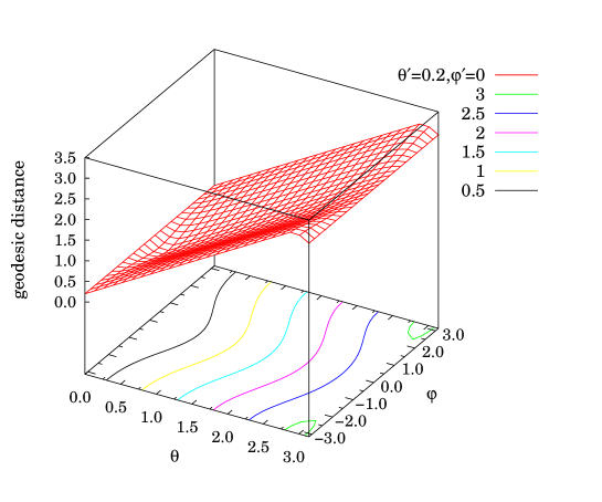
Figure 1: (color online) Three dimensional plot of the geodesic distance of Eq. (6) for $\theta^{\prime}=0.2$ and $\varphi^{\prime}=0$. From the surface graph we see how in proximity of the poles the geodesic distance between points moving along parallels is small while it increases rapidly if one moves along the meridians.

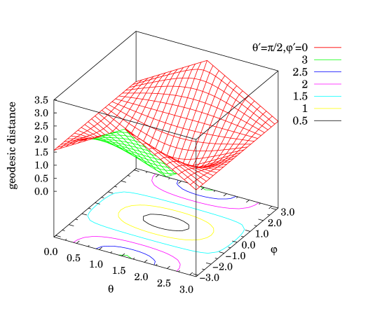
Figure 2: (color online) Three dimensional plot of the geodesic distance of Eq. (6) for $\theta^{\prime}=\pi/2$ and $\varphi^{\prime}=0$. From the surface graph we see how in proximity of the equator the geodesic distance between points moving in circles in the $(\theta,\varphi)$ plane is small while it increases rapidly if one moves along the parallels.

Clearly if we rotate the sphere the paths shape will simply rotate following the rotation of her poles. This anisotropy of the path conformations is rather counter intuitive since the sphere is notoriously isotropic but it reflects the inhomogeneity of the metric respect to the polar angle.

It is important to distinguish the effect that we just described due to the weight factor $\propto\exp(-\hbar ds^{2}/4\lambda\tau)$ stemming from the kinetic part of the primitive action from the measure factor $\prod_{j=1}^{M}\sqrt{\tilde{g}(j)}$ also entering the path integral. This last factor being also independent of the azimuthal angles will produce the same local density $\rho(\mathbf{q})$ under a rotation of the sphere around her axis through the poles. So, by isotropy, we conclude that the density must be a constant under any rotation, which means that the plasma must be uniform [36].

The temperature dependence can also be easily explained. at high temperature $\beta$ is small, $\Theta\gg 1$, and the path extending from $t=0$ to $t=\hbar\beta$ will be localized, of a small size, and quantum effects will be less relevant, whereas at low temperature $\beta$ is large, $\Theta\ll 1$, and the path will be delocalized, increased in size, it diffuses more on the surface, and quantum effects are more relevant. Usually we will be interested in measuring observables which are diagonal so that when dealing with the diagonal density matrix $\rho_{F}(\mathbf{Q},\mathbf{Q};\beta)$ we will observe ring paths such that $\mathbf{Q}(0)=\mathbf{Q}(\hbar\beta)$. Moreover at high temperature the diagonal density matrix will involve almost straight localized ring paths closing themselves on the identity permutation. Whereas at low temperature the delocalized paths will eventually wind through the $\hbar\beta$ periodicity by means of several different permutations ${\cal P}$, so that $\mathbf{Q}(0)={\cal P}\mathbf{Q}(\hbar\beta)$ and so on. Any permutation can be broken into a product of cyclic permutations. Each cycle corresponds to several paths “cross-linking” and forming a larger ring path. Quantum mechanically the plasma does this to lower its kinetic energy. According to Feynman’s 1953 theory [38], the superconductor transition is represented by the formation of macroscopic paths, i.e., those stretching across the whole sphere and involving on the order of N electrons. Or in other words, those ring paths percolating through the periodic boundary conditions $\theta=\theta+\pi$ and $\varphi=\varphi+2\pi$ by means of permutations.

In Fig. 3 we show a snapshot of the macroscopic path during a simulation of Ref. [1].

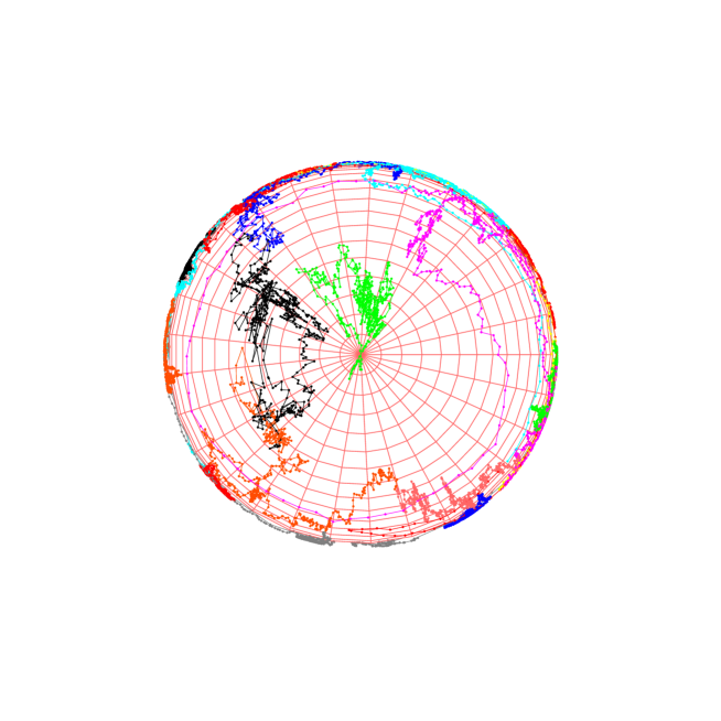
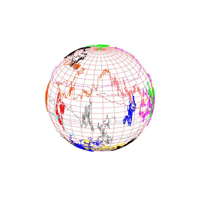
Figure 3: (color online) Snapshot of the macroscopic path during a simulation. The different paths have different colors. The simulation parameter specifying the thermodynamic condition are as follows: $a=5,\lambda=1,\beta=5,\mu=8$.

IV Conclusions

In this work we revised our restricted path integral Monte Carlo simulation [1] of a one-component spinless fermion plasma at finite, non-zero, temperature on the surface of a sphere. The Coulomb interaction is $e^{2}/r$ with $r$ the Euclidean distance between the two electrons of elementary charge $e$ (we could as well have chosen instead of $r$ the geodesic distance, $s$, within the sphere). This gives us an approximated numerical solution of the many-body problem. The exact solution cannot be accessed due to the fermion sign catastrophe. Impenetrable indistinguishable particles on the surface of a sphere admit, in general, anyonic statistics [43]. Here we just project the larger bride group onto the permutation group and choose the fermion sector for our study.

The path integral Monte Carlo method chosen in Ref. [1] used the primitive approximation for the action which could be improved for example by the use of the pair-product action [38]. The restriction was carried on choosing as the trial density matrix the one of ideal free fermion. This choice would of course return an exact solution for the simulation of ideal fermions but it furnishes just an approximation for the interacting coulombic plasma.

In this work we showed how the conformation anisotropy of the paths observed in the simulations of Ref. [1] can be explained through the inhomogeneous nature of the metric in the polar angle. Or equivalently from the inhomogeneous nature of the geodesic distance on the surface of the sphere. And this is ultimately due to the fact that the metric enters with the negative sign in the exponent of the primitive approximation of the density matrix. We should not confuse the anisotropy in the paths conformation with the fact that the plasma will always be homogeneous (with a constant local density $\rho$) on the sphere. In the degenerate regime (low $T$) the observed strong anisotropy in the path conformation near the poles or the equator of the sphere should also be due to a peculiar behavior in the properties of the $N$-particle off-diagonal density matrix. This, as it is well known, is directly related with a number of physical properties, like the quasi-particle excitation spectrum and the momentum distribution. Therefore, the system properties can deviate significantly from just a pure homogeneous 2D system, and the inhomogeneous nature of the space metric is of a particular importance.

We also suggested the possibility to observe a superconducting plasma at low temperature when we observe ring paths percolating through the periodic boundary conditions $\theta=\theta+\pi$ and $\varphi=\varphi+2\pi$ by means of permutations, even if some care has to be addressed to take into account the peculiar asymptotic behavior of the one-particle density matrix.

References

- Fantoni [2018a] R. Fantoni, “One-component fermion plasma on a sphere at finite temperature,” Int. J. Mod. Phys. C 29, 1850064 (2018a).
- Fantoni, Jancovici, and Téllez [2003] R. Fantoni, B. Jancovici, and G. Téllez, “Pressures for a one-component plasma on a pseudosphere,” J. Stat. Phys. 112, 27 (2003).
- Fantoni and Téllez [2008] R. Fantoni and G. Téllez, “Two dimensional one-component plasma on a flamm’s paraboloid,” J. Stat. Phys. 133, 449 (2008).
- Fantoni [2012a] R. Fantoni, “Two component plasma in a flamm’s paraboloid,” J. Stat. Mech. , 04015 (2012a).
- Fantoni [2012b] R. Fantoni, “The density of a fluid on a curved surface,” J. Stat. Mech. , 10024 (2012b).
- Fantoni [2016] R. Fantoni, “Exact results for one dimensional fluids through functional integration,” J. Stat. Phys. 163, 1247 (2016).
- Fantoni [2017] R. Fantoni, “The moment sum-rules for ionic liquids at criticality,” Physica A 477C, 187 (2017).
- Fantoni, Salari, and Klumperman [2012] R. Fantoni, J. W. O. Salari, and B. Klumperman, “The structure of colloidosomes with tunable particle density: Simulation vs experiment,” Phys. Rev. E 85, 061404 (2012).
- Fantoni and Tosi [1995] R. Fantoni and M. P. Tosi, “Coordinate space form of interacting reference response function of d-dimensional jellium,” Nuovo Cimento 17D, 1165 (1995).
- Fantoni [2013] R. Fantoni, “Radial distribution function in a diffusion monte carlo simulation of a fermion fluid between the ideal gas and the jellium model,” Eur. Phys. J. B 86, 286 (2013).
- Fantoni [2021a] R. Fantoni, “Jellium at finite temperature using the restricted worm algorithm,” Eur. Phys. J. B 94, 63 (2021a).
- Fantoni [2021b] R. Fantoni, “Form invariance of the moment sum-rules for jellium with the addition of short-range terms in the pair-potential,” Indian J. Phys. 95, 1027 (2021b).
- Fantoni [2021c] R. Fantoni, “Jellium at finite temperature,” Mol. Phys. 120, 4 (2021c).
- Rashid and Yusoff [2015] A. Rashid and M. Yusoff, eds., Graphene-based Energy Devices (Wiley-VCH, Weinheim, 2015).
- Tiwari and Syväjärvi [2015] A. Tiwari and M. Syväjärvi, eds., Graphene Materials: Fundamentals and Emerging Applications (Scrivener Publishing, Salem, Massachusetts, 2015).
- Guo, Song, and Chena [2010] P. Guo, H. Song, and X. Chena, “Hollow graphene oxide spheres self-assembled by w/o emulsion,” J. Mater. Chem. 20, 4867 (2010).
- Cao et al. [2013] J. Cao, Y. Wang, P. Xiao, Y. Chen, Y. Zhou, J.-H. Ouyang, and D. Jia, “Hollow graphene spheres self-assembled from graphene oxide sheets by a one-step hydrothermal process,” Carbon 56, 389 (2013).
- Wu et al. [2013] L. Wu, H. Feng, M. Liu, K. Zhang, and J. Li, “Graphene-based hollow spheres as efficient electrocatalysts for oxygen reduction,” Nanoscale 5, 10839 (2013).
- Shao et al. [2013] Q. Shao, J. Tang, Y. Lin, F. Zhang, J. Yuan, H. Zhang, N. Shinyaa, and L.-C. Qinc, “Synthesis and characterization of graphene hollow spheres for application in supercapacitors,” J. Mater. Chem. A 1, 15423 (2013).
- Zhao, Chen, and Wu [2016] Y. Zhao, M. Chen, and L. Wu, “Recent progress in hollow sphere-based electrodes for high-performance supercapacitors,” Nanotechnology 27, 342001 (2016).
- Cho, Lee, and Y.C.Kang [2016] J. S. Cho, J.-K. Lee, and Y.C.Kang, “Graphitic carbon-coated fese2 hollow nanosphere-decorated reduced graphene oxide hybrid nanofibers as an efficient anode material for sodium ion batteries,” Scientific Reports 6 (2016).
- Hao et al. [2016] D. Hao, C. Xuefen, Q. Liangdong, and Z. Xiaohui, “Fabrication, characterization and properties of superparamagnetic reduced graphene oxide/fe3o4 hollow sphere nanocomposites,” Rare Metal Materials and Engineering 45, 1669 (2016).
- Huang et al. [2017] W. Huang, S. Ding, Y. Chen, W. Hao, X. Lai, J. Peng, J. Tu, Y. Cao, and X. Li, “3d nio hollow sphere/reduced graphene oxide composite for high-performance glucose biosensor,” Scientific Reports 7 (2017).
- Bi et al. [2017] E. Bi, H. Chen, X. Yang, F. Ye, M. Yin, and L. Han, “Fullerene-structured mose2 hollow spheres anchored on highly nitrogen-doped graphene as a conductive catalyst for photovoltaic applications,” Scientific Reports 5 (2017).
- Brown et al. [2013] E. W. Brown, B. K. Clark, J. L. DuBois, and D. M. Ceperley, Phys. Rev. Lett. 110, 146405 (2013).
- Brown et al. [2014] E. Brown, M. A. Morales, C. Pierleoni, and D. M. Ceperley, “Quantum monte carlo techniques and applications for warm dense matter,” in Frontiers and Challenges in Warm Dense Matter, edited by F. Graziani et al. (Springer, 2014) pp. 123–149.
- Dornheim et al. [2016a] T. Dornheim, S. Groth, T. Sjostrom, F. D. Malone, W. M. C. Foulkes, and M. Bonitz, Phys. Rev. Lett. 117, 156403 (2016a).
- Dornheim et al. [2016b] T. Dornheim, S. Groth, T. Schoof, C. Hann, and M. Bonitz, “Ab initio quantum monte carlo simulations of the uniform electron gas without fixed nodes: The unpolarized case,” Phys. Rev. B 93, 205134 (2016b).
- Groth et al. [2016] S. Groth, T. Schoof, T. Dornheim, and M. Bonitz, “Ab initio quantum monte carlo simulations of the uniform electron gas without fixed nodes,” Phys. Rev. B 93, 085102 (2016).
- Groth et al. [2017] S. Groth, T. Dornheim, T. Sjostrom, F. D. Malone, W. M. C. Foulkes, and M. Bonitz, Phys. Rev. Lett. 119, 135001 (2017).
- Malone et al. [2016] F. D. Malone, N. S. Blunt, E. W. Brown, D. K. K. Lee, J. S. Spencer, W. M. C. Foulkes, and J. J. Shepherd, “Accurate exchange-correlation energies for the warm dense electron gas,” Phys. Rev. Lett. 117, 115701 (2016).
- Filinov et al. [2015] V. S. Filinov, V. E. Fortov, M. Bonitz, and Z. Moldabekov, “Fermionic path-integral monte carlo results for the uniform electron gas at finite temperature,” Phys. Rev. E 91, 033108 (2015).
- Fantoni [2018b] R. Fantoni, Int. J. Mod. Phys. C 29, 1850028 (2018b).
- Melik-Alaverdian, Bonesteel, and Ortiz [1997] V. Melik-Alaverdian, N. E. Bonesteel, and G. Ortiz, “Fixed-phase diffusion monte carlo study of the quantum-hall effect on the haldane sphere,” Phys. Rev. Lett. 79, 5286 (1997).
- Melik-Alaverdian, Ortiz, and Bonesteel [2001] V. Melik-Alaverdian, G. Ortiz, and N. E. Bonesteel, “Quantum projector method on curved manifolds,” J. Stat. Phys. 104, 449 (2001).
- Fantoni [2012c] R. Fantoni, “The density of a fluid on a curved surface,” J. Stat. Mech. , 10024 (2012c).
- Schulman [1981] L. S. Schulman, Techniques and applications of path integrals (John Wiley & Sons, 1981) chapter 24.
- D. M. Ceperley [1995] D. M. Ceperley, Rev. Mod. Phys. 67, 279 (1995).
- Note [1] For a space of constant curvature there is clearly no effect, as the term due to the curvature just leads to a constant multiplicative factor that has no influence on the measure of the various observables. One might have hoped that certain constrained coordinates, perhaps a relative coordinate in a molecule, would effectively live in a space of variable curvature. Perhaps gravitation will give us the system on which the effect of curvature can be seen, but at present the effect is purely in the realm of theory.
- M. H. Kalos and P. A. Whitlock [2008] M. H. Kalos and P. A. Whitlock, Monte Carlo Methods (Wiley-vch Verlag GmbH & Co. KGaA, Weinheim, 2008).
- Ceperley [1991] D. M. Ceperley, J. Stat. Phys. 63, 1237 (1991).
- Ceperley [1996] D. M. Ceperley, “Path integral monte carlo methods for fermions,” in Monte Carlo and Molecular Dynamics of Condensed Matter Systems, edited by K. Binder and G. Ciccotti (Editrice Compositori, Bologna, Italy, 1996).
- Fantoni [2021d] R. Fantoni, “How should we choose the boundary conditions in a simulation which could detect anyons in one and two dimensions?” J. Low Temp. Phys. 202, 247 (2021d).