On singularly perturbed systems that are monotone with respect to a matrix cone of rank $k$

Abstract

We derive a sufficient condition guaranteeing that a singularly perturbed linear time-varying system is strongly monotone with respect to a matrix cone $C$ of rank $k$. This implies that the singularly perturbed system inherits the asymptotic properties of systems that are strongly monotone with respect to $C$, which include convergence to the set of equilibria when $k=1$, and a Poincaré-Bendixson property when $k=2$. We extend this result to singularly perturbed nonlinear systems with a compact and convex state-space. We demonstrate our theoretical results using a simple numerical example.

I Introduction

Dynamical systems whose flow preserves the ordering induced by a proper cone $K$ are called monotone systems. Such systems play an important role in systems and control theory. We begin by reviewing the classic example that is based on the proper cone $K={\mathbb{R}}^{n}_{+}:=\{x\in{\mathbb{R}}^{n}:x_{i}\geq 0,\;i=1,\dots,n\}$, that is, the non-negative orthant in ${\mathbb{R}}^{n}$. This cone induces a (partial) ordering $\leq$ between vectors $a,b\in{\mathbb{R}}^{n}$ defined by

$$a\leq b\iff b-a\in K\iff a_{i}\leq b_{i},\;i=1,\dots,n.$$

Systems whose flow preserves this ordering are called positive systems [1] or cooperative systems [2] and have a rich theory. In particular, the seminal work of Hirsch [3, 4, 5, 6] (see also the work of Matano in [7, 8]) has led to what is now known as Hirsch’s generic convergence theorem, asserting that the generic precompact orbit of a strongly monotone system approaches the set of equilibria (see Poláčik [9, 10] and Smith-Thieme [11] for an improved version of this result). Angeli and Sontag [12] have extended the notion of a monotone system to a system with inputs and outputs, and showed how monotonicity can be applied to analyze the feedback connection of such systems.

A generalization of monotone systems are systems whose flow preserves the ordering induced by a cone of rank $k$ (abbreviated $k$-cone). A set $C\subset\mathbb{R}^{n}$ is called a $k$-cone if:

1. $C$ is closed,

2. $x\in C\implies\alpha x\in C$ for all $\alpha\in{\mathbb{R}}$,

3. $C$ contains a linear $k$-dimensional subspace, and no linear subspace of a higher dimension.

The notion of a $k$-cone was introduced by Fusco and Oliva [13, 14] in the finite-dimensional case, and by Krasnoselśkii et al. [15] in Banach spaces. To avoid degenerate cases, we will assume also that $C$ has a non-empty interior.

For example, if $P\in{\mathbb{R}}^{n\times n}$ is symmetric with $k$ negative eigenvalues and $n-k$ positive eigenvalues then the set

$$C_{P}^{-}:=\{x\in{\mathbb{R}}^{n}:x^{\mathsf{T}}Px\leq 0\}$$ (1)

is a $k$-cone. Since $C_{P}^{-}$ is defined by the matrix $P$, we refer to it as a matrix $k$-cone. Similarly,

$$C_{P}^{+}:=\{x\in{\mathbb{R}}^{n}:x^{\mathsf{T}}Px\geq 0\}$$

is a matrix $(n-k)$-cone.

In general, a $k$-cone is quite different from a proper cone, as it includes a linear subspace and it is typically not convex. Given a $k$-cone $C$, it is possible to define the relations:

$$a\leq^{\scriptstyle C}b\iff b-a\in C,$$

and

$$a\ll^{\scriptstyle C}b\iff b-a\in\operatorname{{\mathrm{i}nt}}(C),$$

but these are not (partial) orderings. In fact, they are neither antisymmetric nor transitive. A dynamical system is called monotone with respect to (w.r.t.) $C$ if its flow $\Phi$ satisfies

$$a\leq^{\scriptstyle C}b\implies\Phi_{t}(a)\leq^{\scriptstyle C}\Phi_{t}(b)\text{ for all }t\geq 0,$$

and strongly monotone w.r.t. $C$ if, in addition,

$$a\leq^{\scriptstyle C}b,\;a\not=b\implies\Phi_{t}(a)\ll^{\scriptstyle C}\Phi_{t}(b)\text{ for all }t>0.$$

For example, consider the LTI system $\dot{x}=Ax$, with $A\in{\mathbb{R}}^{n\times n}$, and the matrix $k$-cone in (1). Fix $a,b\in{\mathbb{R}}^{n}$ such that $a\leq^{\scriptstyle C_{P}^{-}}b$, that is, $(b-a)^{\mathsf{T}}P(b-a)\leq 0$. Then

$$(\Phi_{t}(b)-\Phi_{t}(a))^{\mathsf{T}}P(\Phi_{t}(b)-\Phi_{t}(a))$$

$$=(\exp(At)(b-a))^{\mathsf{T}}P(\exp(At)(b-a))$$

$$=(b-a)^{\mathsf{T}}\left(P+(PA+A^{\mathsf{T}}P)t+o(t)\right)(b-a),$$

implying that a sufficient condition for the flow to be strongly monotone w.r.t. $C_{P}^{-}$ is that

$$PA+A^{\mathsf{T}}P\preceq-2sP-\sigma I_{n},\text{ for some }s\geq 0,\sigma>0.$$ (2)

This linear matrix inequality (LMI) resembles the Lyapunov equation, but here $P$ is not necessarily positive-definite.

Moreover, Eq. (2) implies that the function $V:{\mathbb{R}}^{n}\to{\mathbb{R}}$ defined by $V(z):=z^{\mathsf{T}}Pz$ satisfies

$$\dot{V}(x(t))\leq-2sV(x(t))-\sigma x^{\mathsf{T}}(t)x(t)$$

along a solution of $\dot{x}=Ax$.

An important observation is that if $K$ is a proper cone then $C:=K\cup(-K)$ is a $1$-cone [14]. Since cooperative systems admit ${\mathbb{R}}^{n}_{+}\cup(-{\mathbb{R}}^{n}_{+})$ as an invariant set, the class of systems that are monotone w.r.t. a $k$-cone naturally includes the classical cooperative (and, more generally, monotone) dynamical systems. However, as noted above there is an essential difference between a $k$-cone, with $k\geq 2$, and a proper cone, and this requires substantially new ideas for exploring the implications of monotonicity w.r.t. a $k$-cone.

As noted by Sanchez [16], there are many important examples of flows that are monotone with respect to a $k$-cone, with $k\geq 2$, including: high-dimensional competitive systems (see, e.g., [17, 18, 19, 20, 21, 22, 23, 24, 25]); systems with quadratic cones like in (1) and associated Lyapunov-like functions (see, for example, [26, 27, 28, 29]); and monotone cyclic feedback systems with negative feedback [30, 31, 32, 33], arising from a wide range of neural and physiological control systems. A recent example of an important system that is monotone with respect to a 2-cone is the antithetic integral feedback system [34].

To the best of our knowledge, condition (2) appeared for the first time in the work of R. A. Smith [35, 36]. He showed that strong monotonicity w.r.t. to a matrix 2-cone implies a Poincaré-Bendixson property: the $\omega$-limit set of a bounded orbit containing no equilibria is a closed orbit. Such a result can be useful in establishing that a dynamical system admits a closed orbit, which is in general not trivial.

Consider a system that is strongly monotone with respect to a (not necessarily matrix) $k$-cone $C$, with $k\geq 2$. A nontrivial orbit $O(a):=\{\Phi_{t}(a):t\geq 0\}$ is called pseudo-ordered if there exist times $\tau_{1}\not=\tau_{2}$ such that $\Phi_{\tau_{1}}(a)\leq^{\scriptstyle C}\Phi_{\tau_{2}}(a)$. Otherwise, it is called unordered. The structure of an $\omega$-limit set of a pseudo-ordered orbit is much more complicated than in the case of a system that is monotone w.r.t. a proper cone, due to the lack of convexity of $C$. Sanchez [16, 37] showed that the closure of any orbit in the $\omega$-limit set of a pseudo-ordered orbit is ordered with respect to $C$, and proved a Poincaré-Bendixson property for pseudo-ordered orbits when $k=2$. Sanchez considered smooth finite dimensional flows, and used the $C^{1}$-Closing Lemma to prove his results. Feng, Wang and Wu [38] considered the more general case of a semiflow on a Banach space, without the smoothness requirement, and proved that the $\omega$-limit set $\omega(x)$ of a pseudo-ordered semiorbit admits a trichotomy: $\omega(x)$ is either ordered; or $\omega(x)$ is contained in the set of equilibria; or $\omega(x)$ possesses a certain ordered homoclinic property.

Recently, Feng, Wang, and Wu [39] proved that a system that is strongly monotone w.r.t. a $k$-cone admits an open and dense subset $D$ of the phase space such that orbits with initial point in $D$ are either pseudo-ordered or convergent to equilibria. This covers the celebrated Hirsch’s Generic Convergence Theorem for $k=1$, and yields a generic Poincaré-Bendixson property for $k=2$. Their approach uses ergodic arguments based on $k$-exponential separation.

Wang, Yao and Zhang [40] also analyzed systems that are strongly monotone w.r.t. a $k$-cone from a measure-theoretic perspective. They showed that prevalent (or, equivalently, almost all) orbits will be pseudo-ordered or convergent to equilibria. This reduces to Hirsch’s prevalent convergence Theorem for $k=1$; and implies an almost-sure Poincaré–Bendixson Theorem in the case $k=2$.

Weiss and Margaliot [41] introduced $k$-cooperative systems, i.e., ODE systems that are strongly monotone with respect to the $k$-cone of vectors in ${\mathbb{R}}^{n}$ with up to $k-1$ sign variations. They showed that $1$-cooperative systems are just cooperative systems, cyclic feedback systems with negative feedback are $2$-cooperative systems, and competitive systems are (up to a coordinate transformation) $(n-1)$-cooperative systems. They also established a strong Poincaré-Bendixson property for strongly $2$-cooperative nonlinear systems, namely, if the ${\omega}$-limit set of a precompact solution does not include an equilibrium point then it is a closed orbit. As noted above, Sanchez [16] proved a Poincaré-Bendixson property for certain trajectories of a system that is strongly monotone with respect to a $2$-cone. The results for 2-cooperative systems are stronger: they apply to every precompact trajectory. See [34] for an application of these results to a closed-loop model from systems biology.

Forni, Sepulchre and their colleagues [42, 43] considered monotone systems w.r.t. a matrix $k$-cone (see (1)) in a systems and control perspective, calling them $k$-dominant systems, and used (2) as the definition of $k$-dominance with rate $s$. Importantly, using the fact that (2) is an LMI, they extended the notion of a system that is monotone w.r.t. a matrix $k$-cone to systems with inputs and outputs, and studied the interconnections of such systems.

Singularly perturbed systems [44], [45, Ch. 11] appear naturally in many control applications. For instance, see [46, 47] for an application to low-gain integral control, and [48] for an application to power systems stability.

Wang and Sontag [49] showed that a singularly perturbed strongly monotone system inherits the generic convergence properties of strongly monotone systems, and demonstrated an application in systems biology. Niu and Xie [50] showed that singularly perturbed systems that are strongly monotone w.r.t. a 2-cone inherit the generic Poincaré-Bendixon property. The results in [49, 50] are based on geometric singular perturbations theory [51, 52].

Here, we consider $k$-dominance for singularly perturbed systems. We derive a new sufficient condition for a singularly perturbed system to be $k$-dominant. Our proof uses standard tools from linear algebra and dynamical systems theory, and does not require the heavy machinery of geometric singular perturbations theory. Another advantage of our approach is that it provides an explicit matrix cone $C_{\mathcal{P}}^{-}$ such that the perturbed system is strongly monotone w.r.t. this cone for all ${\varepsilon}>0$ sufficiently small.

The paper is organized as follows. Section II describes some preliminary results that are used later on. Section III describes our main results, and the final section concludes.

We use standard notation. Vectors [Matrices] are denoted by small [capital] letters. Denote ${\mathbb{R}}_{+}:=\{x\in{\mathbb{R}}\ |\ x\geq 0\}$. A matrix $A\in{\mathbb{R}}^{n\times n}$ is called positive-definite (denoted $A\succ 0)$ if $A$ is symmetric and $x^{\mathsf{T}}Ax>0$ for all $x\in{\mathbb{R}}^{n}\setminus\{0\}$. The inertia of a symmetric matrix $A\in{\mathbb{R}}^{n\times n}$ is the triple

$$\operatorname{{\mathrm{I}n}}(A):=(\nu(A),\zeta(A),\pi(A)),$$

in which $\nu(A)$, $\zeta(A)$ and $\pi(A)$ stand for the number of negative, zero, and positive eigenvalues of $A$, respectively. For example, $\operatorname{{\mathrm{I}n}}(A)=(0,0,n)$ [$\operatorname{{\mathrm{I}n}}(A)=(n,0,0)$] iff $A$ is positive-definite [negative-definite].

II Preliminaries

For the reader’s convenience, we recall some background on singular perturbation theory from [44, Chap. 5].

II-A Singular Perturbation Theory for LTV Systems

Consider the LTV singularly perturbed system

$$\dot{x}(t) =A(t)x(t)+B(t)z(t),$$

$${\varepsilon}\dot{z}(t) =C(t)x(t)+D(t)z(t),$$ (3)

where $x:{\mathbb{R}}_{+}\to{\mathbb{R}}^{n_{r}},z:{\mathbb{R}}_{+}\to{\mathbb{R}}^{n_{f}}$, and ${\varepsilon}>0$ small.

Assumption 1.

There exists $c_{1}>0$ such that

$$\mathrm{Re}(\lambda(D(t)))\leq-c_{1}<0\text{ for all }t\geq 0.$$

Assumption 2.

The matrices $A(t),B(t),C(t),D(t)$ are continuously differentiable, bounded, and with bounded derivatives for all $t\geq 0$.

Theorem 3.

[44, Theorem 3.1 (Ch. 5)] Assume that the matrices $A,B,C,D$ satisfy Assumptions 1 and 2. Then, there exists an ${\varepsilon}^{*}>0$ such that for all ${\varepsilon}\in(0,{\varepsilon}^{*})$ there exist continuously differentiable matrices $L_{\varepsilon}(t)$ and $H_{\varepsilon}(t)$, bounded for all $t\geq 0$, satisfying

$${\varepsilon}\dot{L}_{\varepsilon} =DL_{\varepsilon}-C-{\varepsilon}L_{\varepsilon}(A-BL_{\varepsilon}),$$ (4)

$$-{\varepsilon}\dot{H}_{\varepsilon} =H_{\varepsilon}D-B+{\varepsilon}H_{\varepsilon}L_{\varepsilon}B-{\varepsilon}(A-BL_{\varepsilon})H_{\varepsilon}.$$ (5)

Moreover,

$$L_{\varepsilon}=L_{0}+O({\varepsilon}),\quad H_{\varepsilon}=H_{0}+O({\varepsilon}),$$ (6)

with $L_{0}:=D^{-1}C$, $H_{0}:=BD^{-1}$.

Under the assumptions of Theorem 3, the matrix

$$T_{\varepsilon}(t):=\left[\begin{matrix}I_{n_{r}}&{\varepsilon}H_{\varepsilon}(t)\\ -L_{\varepsilon}(t)&I_{n_{f}}-{\varepsilon}L_{\varepsilon}(t)H_{\varepsilon}(t)\end{matrix}\right],$$ (7)

is well-defined and non-singular for all $t\geq 0$. Introducing the state-variables $\left[\begin{smallmatrix}\xi\\ \eta\end{smallmatrix}\right]:=(T_{\varepsilon})^{-1}\left[\begin{smallmatrix}x\\ z\end{smallmatrix}\right]$ transforms the singularly perturbed LTV system (II-A) to the decoupled system:

$$\begin{bmatrix}\dot{\xi}\\ \dot{\eta}\end{bmatrix}=\mathcal{A}_{\varepsilon}(t)\begin{bmatrix}\xi\\ \eta\end{bmatrix},$$ (8)

with

$$\mathcal{A}_{\varepsilon}(t):=\left[\begin{matrix}A(t)-B(t)L_{\varepsilon}(t)&0\\ 0&{\varepsilon}^{-1}D(t)+L_{\varepsilon}(t)B(t)\end{matrix}\right].$$ (9)

Remark 4.

It can be verified that $\det(T^{-1}_{\varepsilon}(t))=1$ for all $t\geq 0$ and all ${\varepsilon}>0$. Moreover, $T_{\varepsilon}$ is a Lyapunov transformation, namely, it is stability-preserving (see [44, Ch. 5] for more details).

Remark 5.

Theorem 3 guarantees that the matrices $L_{\varepsilon}(t)$ [$H_{\varepsilon}(t)$] converge when ${\varepsilon}\to 0$ to $L_{0}$ [$H_{0}$] (uniformly in $t\geq 0$), i.e., to the solutions of (4) obtained by setting ${\varepsilon}=0$.

The reduced (slow) model associated to (II-A) is

$$\dot{x}_{s}(t)=A_{0}(t)x_{s}(t),\text{ with }A_{0}(t):=A(t)-B(t)L_{0}(t),$$ (10)

while the boundary-layer (fast) systems is given by

$${\varepsilon}\dot{z}_{f}(t)=D(t)z_{f}(t),$$ (11)

where here $t\geq 0$ is treated as a fixed parameter.

Singular perturbation theory allows to deduce the stability of (II-A) based on properties of the slow and fast systems. The next result demonstrates this.

Theorem 6.

[44, Theorem 4.1 (Ch. 5)] Assume that the matrices $A,B,C,D$ in (II-A) satisfy Assumptions 1 and 2. Further, assume that the slow system (10) is uniformly asymptotically stable. Then, there exists an ${\varepsilon}^{*}>0$ such that for any ${\varepsilon}\in(0,{\varepsilon}^{*})$ the singularly perturbed system (II-A) is uniformly asymptotically stable. In particular, the state transition matrix $\phi_{{\varepsilon}}$ of (II-A) satisfies

$$\|\phi_{{\varepsilon}}(t,s)\|\leq me^{-\alpha(t-s)}\text{ for all }t\geq s\geq 0,$$

for some $m,\alpha>0$ that are independent of ${\varepsilon}$.

The proof of this theorem is based on using $T_{\varepsilon}$ in (7) to transform (II-A) into (8), and observing that $\xi$ is a regular perturbation of the uniformly asymptotically stable (slow) system (10) (see Theorem 3). Similarly, the stability of $\eta$ is linked to that of the fast variable $z_{f}$ in (11). For a detailed proof, we refer the reader to [44, Sec. 5.2].

III Main results

This section includes our main results.

III-A $p$-Dominance of a Singularly Perturbed LTV System

Our first result provides a sufficient condition for $p$-dominance of (II-A).

Theorem 7.

Consider the singularly perturbed LTV system (II-A), with $A,B,C,D$ satisfying Assumption 2. Suppose that there exist symmetric matrices $P_{r}\in{\mathbb{R}}^{n_{r}\times n_{r}}$ with $\operatorname{{\mathrm{I}n}}(P_{r})=(p,0,n_{r}-p)$, and $P_{f}\in{\mathbb{R}}^{n_{f}\times n_{f}}$ with $\operatorname{{\mathrm{I}n}}(P_{f})=(0,0,n_{f})$, rates $\lambda_{r},\lambda_{f}\geq 0$ and $\sigma_{r},\sigma_{f}>0$ such that

$$P_{r}A_{0}(t)+A_{0}^{\mathsf{T}}(t)P_{r}\preceq-2\lambda_{r}P_{r}-\sigma_{r}I_{n_{r}},$$ (12a)

$$P_{f}D(t)+D^{\mathsf{T}}(t)P_{f}\preceq-2\lambda_{f}P_{f}-\sigma_{f}I_{n_{f}},$$ (12b)

for all $t\geq 0$. Let $\mathcal{P}:=\begin{bmatrix}P_{r}&0\\ 0&P_{f}\end{bmatrix}$. Then there exists ${\varepsilon}^{*}>0$ such that for any ${\varepsilon}\in(0,{\varepsilon}^{*})$, system (II-A) is $p$-dominant w.r.t. $\mathcal{P}$ with rate $\lambda_{r}$.

Note that (12a) is a $p$-dominance condition for the reduced model (10). Since $P_{f}$ is positive-definite, (12b) is a contraction condition on the fast system (11) w.r.t. to a scaled $L_{2}$ norm (see, e.g., [53, 54]). This latter condition is a “strong version” of Assumption 1.

Proof.

Eq. (12b) implies that Assumption 1 holds, so by Theorem 3 it is enough to analyze (8). Let $\sigma:=(1/2)\min\{\sigma_{r},\sigma_{f}\}>0$. We claim that there exists ${\varepsilon}^{*}>0$ such that for any ${\varepsilon}\in(0,{\varepsilon}^{*})$, we have

$$\mathcal{P}\mathcal{A}_{\varepsilon}(t)+\mathcal{A}^{\mathsf{T}}_{\varepsilon}(t)\mathcal{P}\preceq-2\lambda_{m}\mathcal{P}-\sigma I_{n_{r}+n_{f}},$$

for all $t\geq 0$. To simplify the notation, we omit the dependence on $t$ from now on. By the block-diagonal form of $\mathcal{A}_{\varepsilon}$, it is enough to show that for any $t\geq 0$, we have

$$P_{r}(A-BL_{{\varepsilon}})+(A-BL_{{\varepsilon}})^{\mathsf{T}}P_{r}\preceq-2\lambda_{r}P_{r}-\sigma I_{n_{f}},$$ (13)

and

$$P_{f}({\varepsilon}^{-1}D+L_{{\varepsilon}}B)+({\varepsilon}^{-1}D+L_{{\varepsilon}}B)^{\mathsf{T}}P_{f}\\ \preceq-2\lambda_{r}P_{f}-\sigma I_{n_{f}},$$ (14)

Combining (12a), Assumption 2 and (6) implies that (13) holds. Furthermore, since $L_{\varepsilon}$ and $B$ are bounded, it follows from (12b) that the left hand side of (14) can be made arbitrarily negative-definite by taking ${\varepsilon}>0$ small enough, and in particular such that (14) holds, and this completes the proof. ∎

Specializing Theorem 7 to the case of LTI systems yields the following result.

Corollary 8.

Consider the LTI singularly perturbed system:

$$\dot{x}(t) =Ax(t)+Bz(t),$$

$${\varepsilon}\dot{z}(t) =Cx(t)+Dz(t),$$ (15)

with $D$ invertible, and let $A_{0}:=A-BD^{-1}C$. Suppose that there exist symmetric matrices $P_{r},P_{f}\in{\mathbb{R}}^{n\times n}$ with $\operatorname{{\mathrm{I}n}}(P_{r})=(p,0,n_{r}-p)$, $\operatorname{{\mathrm{I}n}}(P_{f})=(0,0,n_{f})$, rates $\lambda_{r},\lambda_{f}\geq 0$, and $\sigma_{r},\sigma_{f}>0$ such that

$$P_{r}A_{0}+A_{0}^{\mathsf{T}}P_{r}\preceq-2\lambda_{r}P_{r}-\sigma_{r}I_{n_{r}},$$ (16a)

$$P_{f}D+D^{\mathsf{T}}P_{f}\preceq-2\lambda_{f}P_{f}-\sigma_{f}I_{n_{f}}.$$ (16b)

Then there exists ${\varepsilon}^{*}>0$ such that for any ${\varepsilon}\in(0,{\varepsilon}^{*})$, system (8) is $p$-dominant with respect to $\mathcal{P}$ with rate $\lambda_{r}$.

In the particular case $p=0$ (so $P_{r}\succ 0$), this implies that for any ${\varepsilon}>0$ sufficiently small the perturbed system is $0$-dominant w.r.t. to the positive-definite matrix $\mathcal{P}$, and thus it is asymptotically stable. This recovers Theorem 6.

III-B $p$-Dominance in a Singularly Perturbed Nonlinear System

We now extend the analysis to time-invariant nonlinear systems. The basic idea is to consider the variational equation associated with the singularly perturbed nonlinear system (this is sometimes referred to as differential analysis or incremental analysis [42, 54, 55]). In our case, the variational system is a singularly perturbed LTV system.

Consider the singularly perturbed nonlinear system

$$\dot{x} =f(x,z),$$

$${\varepsilon}\dot{z} =g(x,z),$$ (17)

where ${\varepsilon}>0$, $f\in C^{2}(\mathbb{R}^{n_{r}}\times\mathbb{R}^{n_{f}};\mathbb{R}^{n_{r}})$, $g\in C^{2}(\mathbb{R}^{n_{r}}\times\mathbb{R}^{n_{f}};\mathbb{R}^{n_{f}})$, and $f(0,0)=0$, $g(0,0)=0$.

We assume that (III-B) admits a compact and convex state-space $\Omega_{x}\times\Omega_{z}\subset{\mathbb{R}}^{n_{r}}\times{\mathbb{R}}^{n_{f}}$ for any ${\varepsilon}>0$. Given an initial condition $\begin{bmatrix}x_{0}\\ z_{0}\end{bmatrix}\in\Omega_{x}\times\Omega_{z}$, the variational system of (III-B) is

$$\begin{gathered}\dot{x}_{\delta}=\frac{\partial f}{\partial x}(x,z)x_{\delta}+\frac{\partial f}{\partial z}(x,z)z_{\delta},\\ {\varepsilon}\dot{z}_{\delta}=\frac{\partial g}{\partial x}(x,z)x_{\delta}+\frac{\partial g}{\partial z}(x,z)z_{\delta},\end{gathered}$$ (18)

where the Jacobians are evaluated along the trajectory $\left[\begin{smallmatrix}x(t)\\ z(t)\end{smallmatrix}\right]\in\Omega_{x}\times\Omega_{z}$ of (III-B). Note that (18) is a singularly perturbed LTV system.

We assume that there exists $h\in C^{2}(\mathbb{R}^{n_{r}};\mathbb{R}^{n_{f}})$ such that $g(x,h(x))=0$ for all $x\in\mathbb{R}^{n_{r}}$. Then, the reduced model associated with (18) is

$$\dot{x}_{s}=\left[\frac{\partial f}{\partial x}(x,z)+\frac{\partial f}{\partial z}(x,z)\frac{\partial h}{\partial x}(x)\right]x_{s},$$ (19)

where

$$\frac{\partial h}{\partial x}(x)=-\left[\frac{\partial g}{\partial z}(x,h(x))\right]^{-1}\frac{\partial g}{\partial x}(x,h(x)).$$ (20)

The boundary-layer associated to (18) is

$${\varepsilon}\dot{z}_{f}=\frac{\partial g}{\partial z}(x,z_{f}+h(x))z_{f},$$ (21)

where here $x\in\mathbb{R}^{n_{r}}$ is treated as a fixed parameter. Let

$$\begin{gathered}A:=\frac{\partial f}{\partial x}(x,z),\quad B:=\frac{\partial f}{\partial z}(x,z),\\ C:=\frac{\partial g}{\partial x}(x,z),\quad D:=\frac{\partial g}{\partial z}(x,z),\end{gathered}$$ (22)

where for simplicity we omit the dependence of $A,B,C,D$ on $(x(t),z(t))$. Let

$$\begin{gathered}L_{0}:=D^{-1}C\quad\text{and}\quad A_{0}:=A-BL_{0}.\end{gathered}$$ (23)

Assumption 9.

The matrices $A,B,C,D$ are continuously differentiable, bounded, and with bounded derivatives for any initial condition $(x_{0},z_{0})\in\Omega_{x}\times\Omega_{z}$ of (III-B).

We can now state our second main result.

Theorem 10.

Consider the singularly perturbed nonlinear system (III-B), and assume that Assumption 9 holds. Suppose that there exist symmetric matrices $P_{r}\in{\mathbb{R}}^{n_{r}\times n_{r}}$ with $\operatorname{{\mathrm{I}n}}(P_{r})=(p,0,n_{r}-p)$, and $P_{f}\in{\mathbb{R}}^{n_{f}\times n_{f}}$ with $\operatorname{{\mathrm{I}n}}(P_{f})=(0,0,n_{f})$, rates $\lambda_{r},\lambda_{f}\geq 0$ and $\sigma_{r},\sigma_{f}>0$ such that

$$P_{r}A_{0}+(A_{0})^{\mathsf{T}}P_{r}\preceq-2\lambda_{r}P_{r}-\sigma_{r}I_{n_{r}},$$ (24a)

$$P_{f}D+D^{\mathsf{T}}P_{f}\preceq-2\lambda_{f}P_{f}-\sigma_{f}I_{n_{f}},$$ (24b)

for all $(x,z)$ emanating from initial conditions $(x_{0},z_{0})\in\Omega_{x}\times\Omega_{z}$ of (III-B). Let

$$\mathcal{P}:=\begin{bmatrix}P_{r}&0\\ 0&P_{f}\end{bmatrix}.$$

Then there exists ${\varepsilon}^{*}>0$ such that for any ${\varepsilon}\in(0,{\varepsilon}^{*})$, the system (III-B) is $p$-dominant w.r.t. $\mathcal{P}$ with rate $\lambda_{r}$.

Proof.

Fix $(x_{0},z_{0}),(\tilde{x}_{0},\tilde{z}_{0})\in\Omega_{x}\times\Omega_{z}$, and let $(x(t),z(t)),(\tilde{x}(t),\tilde{z}(t))$ denote the corresponding solutions of (III-B). Let $v(t):=x(t)-\tilde{x}(t)$, $w(t):=z(t)-\tilde{z}(t)$, $\bar{x}(t,r):=rx(t)+(1-r)\tilde{x}(t)$, and $\bar{z}(t,r):=rz(t)+(1-r)\tilde{z}(t)$, with $r\in[0,1]$. Then

$$\dot{v} =\int_{0}^{1}\frac{\partial f}{\partial x}(\bar{x},\bar{z})\mathop{}\!\mathrm{d}r\;v+\int_{0}^{1}\frac{\partial f}{\partial z}(\bar{x},\bar{z})\mathop{}\!\mathrm{d}r\;w,$$ (25)

$${\varepsilon}\dot{w} =\int_{0}^{1}\frac{\partial g}{\partial x}(\bar{x},\bar{z})\mathop{}\!\mathrm{d}r\;v+\int_{0}^{1}\frac{\partial g}{\partial z}(\bar{x},\bar{z})\mathop{}\!\mathrm{d}r\;w.$$

By Theorem 7, conditions (24) imply that (25) is $p$-dominant for all ${\varepsilon}>0$ sufficiently small. Using the compactness of $\Omega_{x}\times\Omega_{z}$ implies that there exists ${\varepsilon}^{*}>0$ such that (25) is $p$-dominant for all ${\varepsilon}\in(0,{\varepsilon}^{*})$ and all $(x_{0},z_{0})\in\Omega_{x}\times\Omega_{z}$. In other words,

$$\begin{bmatrix}x_{0}\\ z_{0}\end{bmatrix}-\begin{bmatrix}\tilde{x}_{0}\\ \tilde{z}_{0}\end{bmatrix}\in C^{-}_{\mathcal{P}}\setminus\{0\}\implies\begin{bmatrix}x(t)\\ z(t)\end{bmatrix}-\begin{bmatrix}\tilde{x}(t)\\ \tilde{z}(t)\end{bmatrix}\in\operatorname{{\mathrm{i}nt}}(C^{-}_{\mathcal{P}})$$

for all $t>0$, and this completes the proof. ∎

The next example demonstrates Theorem 10 using a singularly perturbed version of a mechanical system with a nonlinear spring from [42].

Example 11.

Consider the non-linear singularly perturbed system:

$$\dot{x}_{1} =x_{2},$$

$$\dot{x}_{2} =v(x_{1})-5z,$$

$${\varepsilon}\dot{z} =x_{2}-z,$$ (26)

where $v:{\mathbb{R}}\to{\mathbb{R}}$ is $C^{2}$, $v(0)=0$, and $v^{\prime}(s)\in[-5,2]$ for all $s\in{\mathbb{R}}$. The associated variational system is the LTV:

$$\dot{\delta x}_{1} =\delta x_{2},$$

$$\dot{\delta x}_{2} =v^{\prime}(x_{1})\delta x_{1}-5\delta z,$$

$${\varepsilon}\dot{\delta z} =\delta x_{2}-\delta z.$$ (27)

We can write this as the LTV system (II-A) with matrices

$$A=\begin{bmatrix}0&1\\ v^{\prime}(x_{1})&0\end{bmatrix},\ B=\begin{bmatrix}0\\ -5\end{bmatrix},\ C=\begin{bmatrix}0&1\end{bmatrix},\ D=-1.$$

Following Sec. II, we define

$$L_{0}:=D^{-1}C=-C,\quad A_{0}:=A-BL_{0}=\begin{bmatrix}0&1\\ v^{\prime}(x_{1})&-5\end{bmatrix}.$$

Clearly, $A_{0}$ is always in the convex hull of the matrices

$$\underline{M}:=\begin{bmatrix}0&1\\ -5&-5\end{bmatrix},\quad\overline{M}:=\begin{bmatrix}0&1\\ 2&-5\end{bmatrix}.$$

We choose

$$P_{r}:=\begin{bmatrix}-5.1987&3.6260\\ 3.6260&6.1987\end{bmatrix}.$$

Then $\operatorname{{\mathrm{I}n}}(P_{r})=(1,0,1)$, and

$$P_{r}\underline{M}+\underline{M}^{\mathsf{T}}P_{r} \preceq-2\lambda_{r}P_{r}-\sigma_{r}I_{2},$$

$$P_{r}\overline{M}+\overline{M}^{\mathsf{T}}P_{r} \preceq-2\lambda_{r}P_{r}-\sigma_{r}I_{2},$$

for $\lambda_{r}=2$, $\sigma_{r}=0.01$, which corresponds to (24a). Similarly, for $P_{f}=1$, $\lambda_{f}=1/2$, and $\sigma_{f}=1$, we have

$$P_{f}D+D^{\mathsf{T}}P_{f}\preceq-2\lambda_{f}P_{f}-\sigma_{f},$$

which corresponds to (24b). We conclude that all the conditions in Theorem 10 hold, so the system is $1$-dominant. Thus, every bounded trajectory converges to an equilibrium point. Fig. 1 depicts several trajectories of (11) with $v(x)=7\tanh(x)-5x$ and ${\varepsilon}=0.01$. It may be seen that indeed every trajectory converges to an equilibrium point.

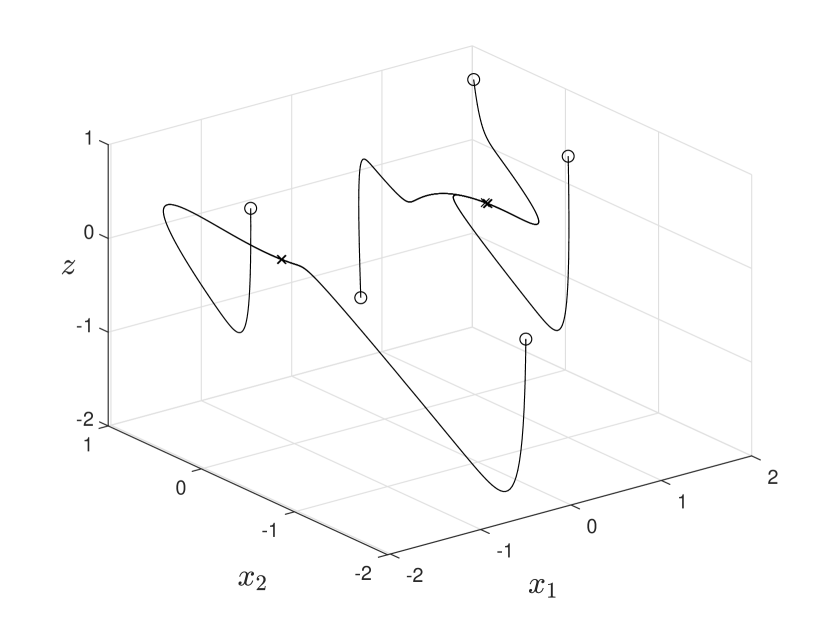
Figure 1: Several trajectories of (11). Initial conditions [equilibrium points] are marked with ’$\circ$’ [’x’].

IV Conclusion

Systems that are monotone w.r.t. a cone of rank $k$ satisfy useful asymptotic properties. This follows from the fact that, roughly speaking, almost all bounded solutions of such a system can be injectively projected into a $k$-dimensional subspace, so essentially the dynamics is $k$-dimensional [16].

We derived a sufficient condition guaranteeing that a singularly perturbed nonlinear system is monotone w.r.t. a matrix cone of rank $k$. The analysis is relatively simple and does not require using geometric singular perturbations theory. Another advantage of our approach is that it provides an explicit expression for the matrix $k$-cone $C_{\mathcal{P}}^{-}$.

We demonstrated our results using a synthetic example, but we believe that it may be useful in the analysis of real-world systems, e.g., power systems. Another possible direction for future research is to study the relation of our results to singularly perturbed $k$-contractive systems.

Acknowledgments

We are grateful to Yi Wang for helpful comments.

References

- [1] L. Farina and S. Rinaldi, Positive Linear Systems: Theory and Applications. Wiley-Interscience, 2000.
- [2] H. L. Smith, Monotone Dynamical Systems: An Introduction to the Theory of Competitive and Cooperative Systems, ser. Math. Surveys and Monographs. Providence, RI: Amer. Math. Soc., 1995, vol. 41.
- [3] M. W. Hirsch, “The dynamical systems approach to differential equations,” Bull. Amer. Math. Soc., vol. 11, pp. 1–64, 1984.
- [4] ——, “Stability and convergence in strongly monotone dynamical systems,” J. Reine Angew. Math., vol. 383, pp. 1–53, 1988.
- [5] ——, “Systems of differential equations which are competitive or cooperative I: Limit sets,” SIAM J. Math. An., vol. 13, pp. 167–179, 1982.
- [6] ——, “Systems of differential equations which are competitive or cooperative II: Convergence almost everywhere,” SIAM J. Math. Anal., vol. 16, pp. 423–439, 1985.
- [7] H. Matano, “Asymptotic behavior and stability of solutions of semilinear diffusion equations,” RIMS, Kyoto Univ., vol. 15, p. 401–454, 1979.
- [8] ——, “Strongly order-preserving local semi-dynamical systems-theory and applications,” in Semigroups, Theory and Applications, H. Brezis, M. Crandall, and F. Kappel, Eds. London: Longman Scientific and Technical, 1986, p. 178–185.
- [9] P. Poláčik, “Convergence in smooth strongly monotone flows defined by semilinear parabolic equations,” J. Diff. Eqns., vol. 79, pp. 89–110, 1989.
- [10] ——, “Generic properties of strongly monotone semiflows defined by ordinary and parabolic differential equations,” in Qualitative theory of differential equations (Szeged 1988). Amsterdam: North-Holland, 1990, pp. 519–530.
- [11] H. Smith and H. Thieme, “Convergence for strongly order-preserving seliflows,” SIAM J. Math. Anal., vol. 22, pp. 1081–1101, 1991.
- [12] D. Angeli and E. Sontag, “Monotone control systems,” IEEE Trans. Automat. Control, vol. 48, no. 10, pp. 1684–1698, 2003.
- [13] G. Fusco and W. Oliva, “Jacobi matrices and transversality,” Proc. R. Soc., Edinb. A, vol. 109, pp. 231–243, 1988.
- [14] ——, “A Perron theorem for the existence of invariant subspaces,” Ann. Mat. Pura Appl., vol. 160, pp. 63–76, 1991.
- [15] M. Krasnoselśkii, E. Lifshits, and A. Sobolev, Positive Linear Systems, the Method of Positive Operators. Berlin: Heldermann Verlag, 1989.
- [16] L. A. Sanchez, “Cones of rank 2 and the Poincaré–Bendixson property for a new class of monotone systems,” J. Diff. Eqns., vol. 246, no. 5, pp. 1978–1990, 2009.
- [17] S. Baigent, “Geometry of carrying simplices of 3-species competitive Lotka-Volterra systems,” Nonlinearity, vol. 26, pp. 1001–1029, 2013.
- [18] ——, “Carrying simplices for competitive maps,” in Difference Equations, Discrete Dynamical Systems and Applications, S. Elaydi, C. Pötzsche, and A. L. Sasu, Eds. Cham, Switzerland: Springer, 2019, p. 3–29.
- [19] M. W. Hirsch, “Systems of differential equations which are competitive or cooperative III: Competing species,” Nonlinearity, vol. 1, pp. 51–71, 1988.
- [20] J. Jiang, J. Mierczyński, and Y. Wang, “Smoothness of the carrying simplex for discrete-time competitive dynamical systems: a characterization of neat embedding,” J. Diff. Eqns., vol. 246, pp. 1623–1672, 2009.
- [21] J. Mierczyński, “The property of convex carrying simplices for competitive maps,” Ergod. Theory Dyn. Syst., vol. 40, pp. 1335–1350, 2020.
- [22] ——, “The property of convex carrying simplices for a class of competitive system of ODEs,” J. Diff. Eqns., vol. 111, pp. 385–409, 1994.
- [23] J. Mierczyński, L. Niu, and A. Ruiz-Herrera, “Linearization and invariant manifolds on the carrying simplex for competitive maps,” J. Diff. Eqns., vol. 267, pp. 7385–7410, 2019.
- [24] J. Jiang and L. Niu, “On the equivalent classification of three-dimensional competitive Leslie/Gower models via the boundary dynamics on the carrying simplex,” J. Math. Biol., vol. 74, pp. 1223–1261, 2017.
- [25] Y. Wang and J. Jiang, “The general properties of discrete-time competitive dynamical systems,” J. Diff. Eqns., vol. 176, pp. 470–493, 2001.
- [26] R. Ortega and L. Sanchez, “Abstract competitive systems and orbital stability in ,” Proc. Amer. Math. Soc., vol. 128, pp. 2911–2919, 2000.
- [27] R. A. Smith, “Existence of periodic orbits of autonomous ordinary differential equations,” Proc. R. Soc., Edinb. A, vol. 85, pp. 153–172, 1980.
- [28] ——, “Orbital stability for ordinary differential equations,” J. Diff. Eqns., vol. 69, pp. 265–287, 1987.
- [29] L. Feng, Y. Wang, and J. Wu, “Generic convergence to periodic orbits for monotone flows with respect to 2-cones and applications to SEIRS models,” SIAM J. Appl. Math., vol. 82, no. 5, pp. 1829–1850, 2022.
- [30] J. Mallet-Paret and R. Nussbaum, “Tensor products, positive linear operators, and delay-differential equations,” J. Dynam. Diff. Eqns., vol. 25, pp. 843–905, 2013.
- [31] J. Mallet-Paret and G. Sell, “The Poincaré-Bendixson theorem for monotone cyclic feedback systems with delay,” J. Diff. Eqns., vol. 125, pp. 441–489, 1996.
- [32] J. Mallet-Paret and H. Smith, “The Poincaré-Bendixson theorem for monotone cyclic feedback systems,” J. Dynam. Diff. Eqns., vol. 2, pp. 367–421, 1990.
- [33] T. Ben-Avraham, G. Sharon, Y. Zarai, and M. Margaliot, “Dynamical systems with a cyclic sign variation diminishing property,” IEEE Trans. Automat. Control, vol. 65, pp. 941–954, 2020.
- [34] M. Margaliot and E. D. Sontag, “Compact attractors of an antithetic integral feedback system have a simple structure,” 2019. [Online]. Available: https://www.biorxiv.org/content/10.1101/868000v1
- [35] R. A. Smith, “The Poincaré–Bendixson theorem for certain differential equations of higher order,” Proc. R. Soc., Edinb. A, vol. 83, no. 1-2, p. 63–79, 1979.
- [36] ——, “Existence of periodic orbits of autonomous ordinary differential equations,” Proc. R. Soc., Edinb. A, vol. 85, pp. 153–172, 1980.
- [37] L. A. Sanchez, “Existence of periodic orbits for high-dimensional autonomous systems,” J. Math. Anal. Appl., vol. 363, pp. 409–418, 2010.
- [38] L. Feng, Y. Wang, and J. Wu, “Semiflows “monotone with respect to high-rank cones” on a Banach space,” SIAM J. Math. Anal., vol. 49, pp. 142–161, 2017.
- [39] ——, “Generic behavior of flows strongly monotone with respect to high-rank cones,” J. Diff. Eqns., vol. 275, pp. 858–881, 2021.
- [40] Y. Wang, J. Yao, and Y. Zhang, “Prevalent behavior and almost sure Poincaré–Bendixson theorem for smooth flows with invariant -cones,” J. Dyn. Diff. Equat., 2022, to appear.
- [41] E. Weiss and M. Margaliot, “A generalization of linear positive systems with applications to nonlinear systems: Invariant sets and the Poincaré-Bendixson property,” Automatica, vol. 123, p. 109358, 2021.
- [42] F. Forni and R. Sepulchre, “Differential dissipativity theory for dominance analysis,” IEEE Trans. Automat. Control, vol. 64, no. 6, pp. 2340–2351, 2018.
- [43] F. A. Miranda-Villatoro, F. Forni, and R. J. Sepulchre, “Analysis of Lur’e dominant systems in the frequency domain,” Automatica, vol. 98, pp. 76–85, 2018.
- [44] P. Kokotović, H. K. Khalil, and J. O’reilly, Singular Perturbation Methods in Control: Analysis and Design. SIAM, 1999.
- [45] H. Khalil, Nonlinear Systems. Prentice Hall, 2002.
- [46] P. Lorenzetti and G. Weiss, “Saturating PI control of stable nonlinear systems using singular perturbations,” IEEE Trans. Automat. Control, vol. 68, no. 2, pp. 867–882, 2023.
- [47] ——, “PI control of stable nonlinear plants using projected dynamical systems,” Automatica, vol. 146, p. 110606, 2022.
- [48] P. Lorenzetti, Z. Kustanovich, S. Shivratri, and G. Weiss, “The equilibrium points and stability of grid-connected synchronverters,” IEEE Trans. on Power Systems, vol. 37, no. 2, pp. 1184–1197, 2022.
- [49] L. Wang and E. D. Sontag, “Singularly perturbed monotone systems and an application to double phosphorylation cycles,” J. Nonlinear Sci., vol. 18, p. 527–550, 2008.
- [50] L. Niu and X. Xie, “Generic Poincaré-Bendixson theorem for singularly perturbed monotone systems with respect to cones of rank-2,” 2021. [Online]. Available: https://arxiv.org/abs/2110.11783v1
- [51] N. Fenichel, “Geometric singular perturbation theory for ordinary differential equations,” J. Diff. Eqns., vol. 31, p. 53–98, 1979.
- [52] K. Sakamoto, “Invariant manifolds in singular perturbation problems for ordinary differential equations,” Proc. R. Soc., Edinb. A, vol. 116, p. 45–78, 1990.
- [53] W. Lohmiller and J.-J. E. Slotine, “On contraction analysis for non-linear systems,” Automatica, vol. 34, pp. 683–696, 1998.
- [54] Z. Aminzare and E. D. Sontag, “Contraction methods for nonlinear systems: A brief introduction and some open problems,” in Proc. 53rd IEEE CDC, Los Angeles, CA, 2014, pp. 3835–3847.
- [55] C. Wu, I. Kanevskiy, and M. Margaliot, “-contraction: theory and applications,” Automatica, vol. 136, p. 110048, 2022.