Data driven approach to sparsification of reaction diffusion complex network systems

Abstract

Graph sparsification is an area of interest in computer science and applied mathematics. Sparsification of a graph, in general, aims to reduce the number of edges in the network while preserving specific properties of the graph, like cuts and subgraph counts. Computing the sparsest cuts of a graph is known to be NP-hard, and sparsification routines exists for generating linear sized sparsifiers in almost quadratic running time $O(n^{2+\epsilon})$. Consequently, obtaining a sparsifier can be a computationally demanding task and the complexity varies based on the level of sparsity required. In this study, we extend the concept of sparsification to the realm of reaction-diffusion complex systems. We aim to address the challenge of reducing the number of edges in the network while preserving the underlying flow dynamics. To tackle this problem, we adopt a relaxed approach considering only a subset of trajectories. We map the network sparsification problem to a data assimilation problem on a Reduced Order Model (ROM) space with constraints targeted at preserving the eigenmodes of the Laplacian matrix under perturbations. The Laplacian matrix ($L=D-A$) is the difference between the diagonal matrix of degrees ($D$) and the graph’s adjacency matrix ($A$). We propose approximations to the eigenvalues and eigenvectors of the Laplacian matrix subject to perturbations for computational feasibility and include a custom function based on these approximations as a constraint on the data assimilation framework. We demonstrate the extension of our framework to achieve sparsity in parameter sets for Neural Ordinary Differential Equations (neural ODEs).
Keywords: Complex systems, Data assimilation, Differential equations, Dimensionality reduction, Sparse matrices, Network theory, Artificial intelligence.

1 Introduction

Modern deep learning frameworks, which utilize recurrent neural network decoders and convolutional neural networks, are characterized by a significant number of parameters. Finding redundant edges in such networks and rescaling the weights can prove very useful; one such work is done as in [9]. Another line of thought involves learning differential equations from data ([34], [35], [28]), where the data generation part is rendered accessible by using sparse neural networks. These types of work find applications in areas like fluid dynamics, see [45]. Reducing the number of parameters in neural ODEs (ODENets) which can be used to model many complex systems is another motivation for this work.

We define a graph $G=(V,E,w)$ where $V$, $E$ denote the set of vertices and edges of the graph and ${w}$ denotes the weight function, that is ${w}:V\times V\rightarrow\mathbb{R}$. A sparsifier of a graph aims at reducing the number of edges in the graph such that the new reweighted graph $\bar{G}=(V,\bar{E},\bar{w})$ achieves a specific objective like preserving quadratic form of the Laplacian matrix, cuts, subgraph counts. E.g., In the case of spectral sparsifiers, we have

$$\begin{split}\frac{x^{T}Lx}{(1+\epsilon)}\leq\,x^{T}\bar{L}x\leq\,(1+\epsilon)x^{T}Lx\;\;\forall\,x\in\mathbb{R}^{n},\;\;\\ \textrm{where}\;|V|=n,\epsilon\in(0,1).\\ \end{split}$$

The notion of cut sparsification, which produces weighted subgraphs for which each cut is approximated, was introduced by Karger ([18],[19]). The idea involves sampling individual edges of the graph with probability $p$; the resulting sparsifier has size $O(pm)$, where $m=|E|$, the cardinality of the set of edges of the graph. An improved work for producing cut sparsifiers was based on the non-uniform sampling of edges as shown in ([6],[5]). There are other types of sparsifiers which preserve subgraph counts, described as in [1]. Spectral sparsifiers are a more robust form of sparsifiers compared to cut sparsifiers. They aim to preserve the Laplacian quadratic form, as described in [42].

Spielman and Teng introduced a more advanced form of sparsification known as spectral sparsifiers ([42]). Spectral sparsifiers approximate the quadratic form of the graph Laplacian matrix. Such sparsifiers help in solving systems of linear equations ([41], [42]). The resulting sparsified graph exhibits an edge count approximated as $O(n\log(n)^{c}$), where $c$ is a large constant. In their study, Spielman and Srivastava ([40]) demonstrated that it is possible to construct a sparsifier for any graph with $n$ vertices, containing $O(\frac{n\log(n)}{\epsilon^{2}}$) edges. Additionally, they introduced a linear algorithm to achieve this objective. Another work by Goyal, Rademacher and Vempala ([16]) proposed to create cut sparsifiers from random spanning trees. Batson, Spielman and Srivastava ([4]) construct sparsifiers with size $O(\frac{n}{\epsilon^{2}}$) edges in $O(\frac{mn^{3}}{\epsilon^{2}}$) time using a determinstic algorithm. Fung and Harvey devised an algorithm that samples edges based on the inverse of edge connectivity to produce cut sparsifiers ([14]). Additionally they also describe an approach to produce cut sparsifiers from uniformly random spanning trees. A meta-learning-based approach for graph sparsification is discussed in ([44]). The use of sparsification routines, as discussed in ([2]), enables the creation of linear-sized sparsifiers in nearly quadratic time. This approach addresses the sparsification problem by treating it as a regret minimization problem.

We present literature that focuses on preserving the dynamic nature of dynamical systems. The paper by Cencetti, Clusella, and Fanelli ([12]) explores methods for altering the network’s topology while maintaining its dynamic characteristics intact; the new network obtained was isodynamic to the former. Kumar, Ajayakumar and Raha, in their work ([21]), provide mathematical conditions for finding stable bi-partitions of a complex network and also provide a heuristic algorithm for the same. Graph partitioning does not alter the edge weights of graphs; however, it can cause the deletion of edges. This work shows that constrained internal patch dynamics with sufficient network connectivity ensures stable dynamics in subnetworks around its co-existential equilibrium point.

Contributions of our paper: Techniques to rewire the edges of the graph while preserving isodynamic behaviour for complex systems have been discussed in [12]. However, eliminating redundant edges of the graph while preserving the isodynamic behaviour of such complex systems by making use of observational data points in reduced dimension using dimensionality reduction techniques like Proper Orthogonal decomposition (POD) are the main contributions of our work. The problem of sparsification is approached as a Data assimilation problem with constraints. Decision variables are the unknown weights of the graph. The objective is to make this vector of weights as sparse as possible. If the perturbed Laplacian matrix has many eigenmodes similar to the eigenmodes of the given network, patterns produced in the new graph would be highly correlated to the patterns in the network ([12]). Generating eigenvalues and eigenvectors at each iteration of the optimization process is computationally intensive. To overcome this, we propose scalable algorithms which generates approximations to the eigenvalue and eigenvector for the Laplacian matrix subject to perturbations.

The structure of the article is as follows: we begin by presenting some background material from spectral graph theory. A brief overview of reaction-diffusion systems on graphs is provided in the next section. We briefly introduce the adjoint method for data assimilation, which can be applied to the parameter estimation problem. In the subsequent sections, we present the reduced vector field for the chemical Brusselator reaction-diffusion system on the graph and discuss various performance metrics. Challenges involved in ensuring isodynamic behaviour are presented in the next section, the challenging aspect being getting good estimates of the eigenpair of the perturbed Laplacian matrix iteratively. We explore approximations of the eigenpair and their effectiveness in the next section, followed by formulating the optimization problem and its challenges. We present experimental results on real-world graphs to demonstrate the effectiveness of our approach. In Section 8, we show how to produce sparse neural ODENets using the framework for a linear dynamical system.

2 Background

2.1 Laplacian matrix:($L$)

The Laplacian of an undirected weighted graph $G=(V,E)$, where $|V|=n,|E|=m$ with a weight function $w:V\times V\rightarrow\mathbb{R}$ is given by

$$L\left(u,v\right)=\;\left\{\begin{array}[]{ll}d_{v}-w\left(u,v\right)&\mathrm{if}\;u=v,\\ -w\left(u,v\right)&\mathrm{if}\;u\;\mathrm{and}\;v\;\mathrm{are}\;\mathrm{adjacent},\\ 0&\mathrm{otherwise}\ldotp\end{array}\right.$$

Where $d_{v}=\sum_{u\sim v}w(u,v)$ denotes the degree of vertex $v$.

2.2 Incidence matrix:($B$)

The incidence matrix $B_{m\times n}$ with a given orientation of edges of a graph is given by

$$B\left(e,v\right)=\;\left\{\begin{array}[]{ll}1&\mathrm{if}\;v\;\mathrm{is}\;e^{\prime}s\;\mathrm{head},\\ -1&\mathrm{if}\;v\;\mathrm{is}\;e^{\prime}s\;\mathrm{tail},\\ 0&\mathrm{otherwise}\ldotp\end{array}\right.$$

The graph Laplacian matrix for a given orientation with weights $\bar{w}_{i}=\gamma_{i}w_{i},\;i=1,2,\ldots,m$ can be expressed as

$$\begin{split}L=B^{T}W^{1/2}\textrm{diag}(\gamma)W^{1/2}B\quad\textrm{, where }\gamma\in\mathbb{R}^{m}\textrm{ represents the multipliers of the weights},\\ \end{split}$$

$W$ represents the diagonal matrix of weights $w_{i},\;i=1,2,\ldots,m.$

3 Dynamical systems involving graphs

The general form of a reaction-diffusion system is outlined below, as presented in the work of Cencetti et al ([12]). Each node in the network, denoted as $j$, possesses an $\mathrm{m}$-dimensional variable $r_{j}(t)\in\mathbb{R}^{\mathrm{m}}$ that characterizes its activity at time $t$. The evolution of $r_{j}$ over time follows a specific set of rules, beginning from an initial state $r_{j}(0)$ as described below

$$\frac{dr_{j}}{dt}=\mathcal{F}(r_{j})+K\sum_{k=1}^{N}A_{jk}\mathcal{G}(r_{k}-r_{j})\hskip 14.22636ptj=1,2,....N$$

Here $\mathcal{F}$ denotes the reaction component, and the remaining terms account for the diffusion in the graph. $\mathcal{F}:\mathbb{R}^{\mathrm{m}}\rightarrow\mathbb{R}^{\mathrm{m}}$, $\mathcal{G}:\mathbb{R}^{\mathrm{m}}\rightarrow\mathbb{R}^{\mathrm{m}}$. One such Reaction-diffusion system is given by the alternating self-dynamics Brusselator model (Figure 1) where we couple the inter-patch dynamics using the graph Laplacian matrix,

$$\left\{\begin{array}[]{l}\dot{x}_{i}\;=\;a-\left(b+d\right)x_{i}+c\;x_{i}^{2}y_{i}-D_{x}\;\sum_{j}L{\;}_{\mathrm{ij}}x_{j}\\ {\dot{y}_{i}\;=\;\mathrm{b}}x_{i}-c\;x_{\;i}^{2}y_{i}-D_{y}\;\sum_{j}L_{\mathrm{ij}}\;y_{j}\end{array}\right.$$ (1)

With $r_{i}=(x_{i},y_{i})\in\mathbb{R}^{2}$. The system as defined by Equation (1) has fixed points

$$r^{\star}=(x_{i},y_{i})=(\frac{a}{d},\frac{bd}{ac})\,\forall\,i.$$

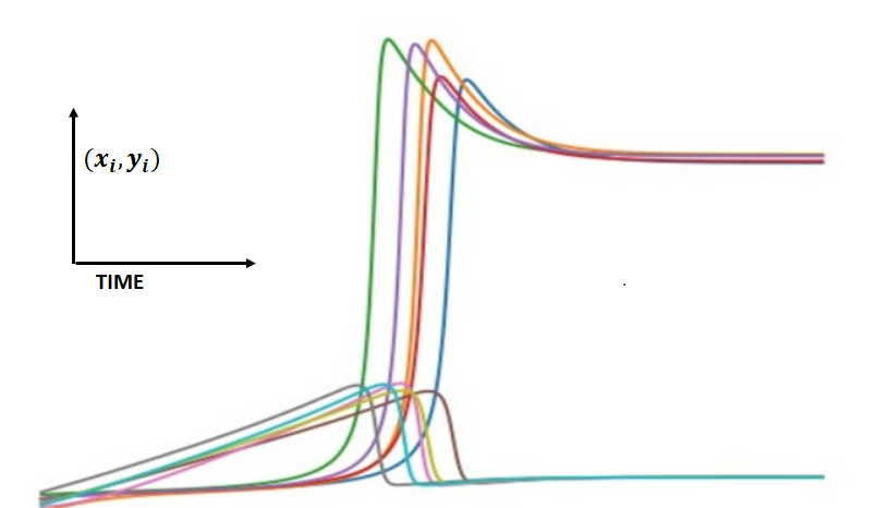
Figure 1: Brusselator dynamics

Our primary objective is to find a graph $\bar{G}=(V,\bar{E},\bar{w})$ with a new sparse weight function $\bar{w}$ such that on solving Equation (1) using the updated graph $\bar{G}$ we get solutions $\bar{x_{i}}\in B(x_{i},\delta_{i}),\bar{y_{i}}\in B(y_{i},\Delta_{i})\;\forall\;i$, where $\delta_{i}$ and $\Delta_{i}$ are relatively small. We will demonstrate the problem on a linear dynamical system involving the Laplacian matrix. The heat kernel matrix involving the Laplacian matrix is given as follows,

$$H_{t}=e^{-Lt}$$ (2)

Differentiating Equation (2) with respect to time, we get

$$\frac{dH_{t}}{dt}=-LH_{t}.$$

This system can be considered a system of odes of the form

$$\hskip 71.13188pt\frac{d\mathcal{F}(x,t)}{dt}=-L\mathcal{F}(x,t)$$ (3)

According to the fundamental Theorem of linear systems, we know that the solution to such a system with initial condition $\mathcal{F}(x,0)=f(x)$ is $\mathcal{F}(x,t)=e^{-Lt}f(x)$ and this solution is unique. The underlying quantity which follows ODE described in Equation (3) could be temperature, chemical reactants, and ecological species. If we use an approximation for $L$, let it be $\bar{L}$ in the above equation with the same initial condition, the solution turns out to be solutions to the ode of the form

$$\hskip 71.13188pt\frac{\partial\bar{\mathcal{F}}}{dt}=-\bar{L}\bar{\mathcal{F}}$$ (4)

$\bar{\mathcal{F}}(x,t)=e^{-\bar{L}t}f(x)$. The error in this substitution at node $x$ for a time $t$ is given by

$$H(x,t)=\mathcal{F}(x,t)-\bar{\mathcal{F}}(x,t),$$

$$H(x,t)=(\sum_{k=1}^{\infty}\frac{{L}^{k}(-t)^{k}}{k!})f(x)-(\sum_{k=1}^{\infty}\frac{{\bar{L}}^{k}(-t)^{k}}{k!})f(x).$$

Given some random initial conditions {$\mathcal{F}_{0\alpha}\}\in\mathbb{R}^{n},\alpha=1,2....,\omega$, one could discretize system as described by Equation (4) to obtain solutions at various time points using a numerical scheme. The discretization of the dynamics for the system described by Equation (4) is as follows,

$$\hskip 14.22636pt\bar{\mathcal{F}}^{\alpha}_{q+1}=M(\bar{\mathcal{F}}^{\alpha}_{q},\bar{w})$$ (5)

where $M:\mathbb{R}^{n}\times\mathbb{R}^{m}\rightarrow\mathbb{R}^{n}$ with $M=(M_{1},M_{2},.....,M_{n})^{T},M_{i}=M_{i}(\bar{\mathcal{F}}^{\alpha}_{q},\bar{w})$ for $1\leq i\leq n$ and $0\leq q\leq S$, $S$ denotes the last time-step, and $\bar{\mathcal{F}}^{\alpha}_{0}\in\mathbb{R}^{n}$ is the initial condition which is assumed to be known. The primary objective would be to obtain a sparse vector of weights $\bar{w}$ which minimizes the error $H$ as explained above, subject to the discrete dynamics shown in Equation (5). This forms the core of the data assimilation problem. To know more about data assimilation, one could refer to ([27], [39], [24]).

4 Adjoint method for data assimilation

Parameter estimation problems have rich literature ([32], [11], [3], [8]). Using Unscented and Extended Kalman filtering-based approaches are not recommended when constraints on parameters are imposed ([33]). We use the Adjoint sensitivity method for the parameter estimation ([23]). In this section, we provide a brief overview of this method and how it could be used in parameter estimation.
Statement of the Inverse Problem: The objective is to estimate the optimal control parameter $\alpha$ that minimizes the cost function $J(\alpha)$ based on a given set of observations $\{\textbf{$z_{k}$}\in\mathbb{R}^{n}\mid 1\leq k\leq N\}$. These observations represent the true state, and the model state $x_{k}$ follows a specific relationship described by $x_{k}=M(x_{k-1},\alpha)$. The state variable $x$ belongs to $\mathbb{R}^{n}$, denoted as $x=(x_{1},x_{2},\dots,x_{n})$, and $F:\mathbb{R}^{n}\times\mathbb{R}^{p}\rightarrow\mathbb{R}^{n}$ represents a mapping function. Specifically, $F=(F_{1},F_{2},\dots,F_{n})$ where $F_{i}=F_{i}(x,\alpha)$ for $1\leq i\leq n$ and $\alpha\in$ $\mathbb{R}^{p}$.
Consider the nonlinear system of the type

$$\frac{dx}{dt}=F(x,\alpha)$$ (6)

with $x(0)=c,$ being the initial condition assumed to be known, $\alpha$ is a system parameter assumed to be unknown. The vector $x(t)$ denotes the state of the system at time t, and $F(x,\alpha)$ represents the vector field at point $x$. If each component of $F_{i}$ of $F$ is continuously differentiable in $x$, the solution to the initial value problem (IVP) exists and is unique.

The Equation (6) can be discretized using many schemes ([10]), and the resulting discrete version of the dynamics can be represented as

$$x_{k+1}=M(x_{k},\alpha)$$

The function $M:\mathbb{R}^{n}\times\mathbb{R}^{p}\rightarrow\mathbb{R}^{n}$ can be represented as $M=(M_{1},M_{2},\ldots,M_{n})$, where each $M_{i}=M_{i}(x_{k},\alpha)$ for $1\leq i\leq n$.

Let us define a function $J:\mathbb{R}^{n}\rightarrow\mathbb{R}$ as follows, ([27])

$$J(\alpha)=\frac{1}{2}\sum_{k=1}^{N}<(z_{k}-x_{k}),(z_{k}-x_{k})>$$

4.1 Adjoint sensitivity with respect to parameter $\alpha$

$$\begin{array}[]{l}\delta J(\alpha)\;=\sum_{k=1}^{N}<\eta_{k},\delta x_{k}>\;\;\;\text{\; for more details refer \cite[cite]{[\@@bibref{}{lakshmivarahan_lewis_2010}{}{}]}}\\ \\ \;\;\;\;\;\;\;\;\;\;\;\;=\sum_{k=1}^{N}<\eta_{k},V_{k}\delta\alpha>\\ \\ \;\;\;\;\;\;\;\;\;\;\;\;\;=<\sum_{k=1}^{N}V_{k}^{T}\eta_{k},\delta\alpha>\\ \end{array}$$

$$\text{where \;}V_{k}=A_{k-1}V_{k-1}+B_{k-1}$$ (7)

$$A_{k-1}=D_{k-1}(M(x_{k-1},\alpha))\in\mathbb{R}^{n\times n}\text{\;and\;}B_{k-1}=D_{\alpha}(M(x_{k-1},\alpha))\in\mathbb{R}^{n\times p}.$$

The recursive relation focuses on finding the sensitivity of $J$ with respect to the parameter $\alpha$. Iterating Equation (7), we get

$$\begin{array}[]{l}V_{k}=\sum_{j=0}^{k-1}(\prod_{s=j+1}^{k-1}A_{s})B_{j}\\ \end{array}$$

The above recursive relation deals with the product of sensitivity matrices.
The first variation of $J$ after specific calculations is given by (see [27])

$$\delta J=<\sum_{k=1}^{N}\sum_{j=0}^{k-1}B_{j}^{T}(\prod_{s=k-1}^{j+1}A_{s}^{T})\eta_{k},\delta\alpha>,\;\;\text{where}\;\;\eta_{k}=x_{k}-z_{k},\\ \prod\,\text{denotes reverse product.}$$ (8)

From first principles

$$\delta J=<\nabla_{\alpha}J(\alpha),\delta\alpha>$$

Comparing first principles with Equation (8), we get

$$\nabla_{\alpha}J(\alpha)=\sum_{k=1}^{N}\sum_{j=0}^{k-1}B_{j}^{T}(\prod_{s=k-1}^{j+1}A_{s}^{T})\eta_{k}$$

4.1.1 Adjoint method Algorithm

1. Start with $x_{0}$ and compute the nonlinear trajectory $\{x_{k}\}_{k=1}^{N}$ using the model $x_{k+1}=M(x_{k},\alpha)$

2. $\lambda_{N}=\eta_{N}$

3. Compute $\lambda_{j}=A_{j}^{T}\lambda_{j+1}+\bar{\eta_{j}}$ for $j=N-1\text{\;to\;}k$, $\bar{\lambda}_{k}=B_{k-1}^{T}\lambda_{k}$, $k=1\text{\;to\;}N$, $\bar{\eta}_{j}=\delta_{j,j_{i}}\eta_{j}$ with $\delta_{j,j_{i}}=1$ when $j=j_{i}$ , else 0

4. sum = 0, sum = sum + $\bar{\lambda}_{k}$ vectors from $k=1\text{\;to\;}N$

5. $\nabla_{\alpha}J(\alpha)=\text{sum}$

6. Using a minimization algorithm find the optimal $\alpha^{*}$ by repeating steps 1 to 5 until convergence

4.2 Computing the Jacobians $D_{k}\left(M\right)$ and $D_{\alpha}\left(M\right)$

This section discusses how to compute the Jacobian matrices described in Section 4.1. The numerical solution of an ODE at timestep $j+1$($y_{j+1}\approx x_{j+1}$) with slope function $\frac{dx}{dt}=f(t,x)$ given $d$ slopes($k_{d}$), where $x\in\mathbb{R}^{n}$ and $f:\mathbb{R}\times\mathbb{R}^{n}\rightarrow\mathbb{R}^{n}$ is given by $y_{j+1}=y_{j}+b_{1}k_{1}+b_{2}k_{2}+....+b_{d}k_{d}$, where $k_{i}=hf(t+c_{i}h,x+a_{i1}k_{1}+a_{i2}k_{2}+...a_{in}k_{n})$. See [10] to learn more about numerical analysis.

We demonstrate computing $D_{k}(M)$ using an explicit numerical scheme, particularly the Euler forward method on the Lotka-Volterra model.

$$\left\{\begin{array}[]{ll}\begin{array}[]{l}\frac{{\mathrm{dx}}_{1}}{\mathrm{dt}\;}=\alpha x_{1}-\beta x_{1}x_{2}\\ \\ \frac{{\mathrm{dx}}_{2}}{\mathrm{dt}}=\delta x_{1}x_{2}-\gamma x_{2}\\ \\ \end{array}&\end{array}\right.$$

When we apply the standard forward Euler scheme, we obtain

$$x_{k+1}=M(x_{k})$$

where $x_{k}=(x_{1k},x_{2k}),\;\textbf{M}(x_{k})=(M_{1}(x_{k}),M_{2}(x_{k}))$ where

$$\begin{array}[]{l}M_{1}\left(x_{k}\right)=x_{1k}+\left(\Delta t\right)\left(\alpha\,x_{1k}-\beta\,x_{1k}x_{2k}\right)\\ M_{2}\left(x_{k}\right)=x_{2k}+\left(\Delta t\right)(\delta\;x_{1k}x_{2k}-\gamma\,x_{2k})\end{array}$$

It can be seen that

$$D_{k}(M)=A_{k}=\left[\begin{array}[]{cc}1+\Delta t\;\left(\alpha-\beta\;x_{2k}\right)&-\Delta t\;\beta\;x_{1k}\\ \Delta t\;\delta\;x_{2k}&1+\Delta t\;\left(\delta\;x_{1k}-\gamma\;\right)\end{array}\right]$$

$$D_{\alpha}(M)=B_{k}=\left[\begin{array}[]{cccc}\Delta tx_{1k}&\Delta t\left(-x_{1k}x_{2k}\right)&0&0\\ 0&0&-\Delta tx_{2k}&\Delta tx_{1k}{\;x}_{2k}\end{array}\right]$$

4.3 Using reduced order model for dynamical systems

When dealing with graphs of considerable size, the dimensionality of the state vector becomes a concern due to its potential impact on computational efficiency. To address this issue, dimensionality reduction techniques like POD, also known as Karhunen–Lo‘eve, can be applied. The work described in [36] discusses the utilization of POD as a means to alleviate the computational complexity associated with large graph sizes. The procedure requires snapshots of solutions of a dynamical system with a vector field $f$ $\in\mathbb{R}^{n}$.

$$\hskip 14.22636pt\dot{x}=f(x,t)$$ (9)

Using the snapshot solutions, we could create a matrix $\rho$ of projection $\in\mathbb{R}^{k\times n}$ where k denotes the reduced order dimension and the mean $\bar{x}$, see [36] for more details. The reduced order model of the system as described by Equation (9) is then given by

$$\dot{z}=\rho f(\rho^{T}z+\bar{x},t).$$

If we are solving an initial value problem with $x(0)=x_{0}$ , then the reduced model will have the initial condition $z(0)=z_{0}$ , where

$$z_{0}=\rho(x_{0}-\bar{x}).$$

The reduced order model for system as described by Equation (4) given the matrix $\rho$ of projection is

$$\dot{z}=-\rho\bar{L}\rho^{T}z-\rho\bar{L}\bar{x}=\psi(z,\bar{w}).$$

The reduced order model for system described by Equation (1) is obtained as follows.
Notation: If $p$ and $q$ are vectors, then $p\,\odot\,q$ represents element-wise multiplication, and $p^{\circ n}$ raises every element of the vector $p$ to power n. Let $B$ be a matrix $\in\mathbb{R}^{n\times n}$, then $B(1:2,:)$ indicates the first 2 rows of $B$ and all the columns of the matrix $B$.
In the context of approximating the vector field, we introduce the concept of multipliers ($\bar{\gamma}$), as defined in Section 2.2. This concept plays a crucial role in our analysis, $\bar{w}=W\bar{\gamma}$.

$$\dot{z}\qquad = \mathbb{\psi}(z,\bar{\gamma}) f2$$ ()

$$= \rho\;h(z)-D_{x}\;\rho(:,1:n)B^{T}W^{1/2}\mathrm{diag}(\bar{\gamma})W^{1/2}B(\rho^{T}(1:n,:)z+\bar{x}(1:n))$$

$$-D_{y}\;\rho(:,n+1:2n)B^{T}W^{1/2}\mathrm{diag}(\bar{\gamma})W^{1/2}B(\rho^{T}(n+1:2n,:)z+\bar{x}(n+1:2n))$$

$$h(z)=\begin{pmatrix}a\mathrm{1}_{n\times 1}-(b+d)(\rho^{T}(1:n,:)z+\bar{x}(1:n))+c[(\rho^{T}(1:n,:)z+\bar{x}(1:n))^{\circ 2}]\odot\\ (\rho^{T}(n+1:2n,:)z+\bar{x}(n+1:2n))\\ \\ b(\rho^{T}(1:n,:)z+\bar{x}(1:n))-c((\rho^{T}(1:n,:)z+\bar{x}(1:n))^{\circ 2})\odot(\rho^{T}(n+1:2n,:)z\\ +\bar{x}(n+1:2n))\\ \end{pmatrix}$$

$$\nabla_{z}h_{e}{\left(z\right)}^{T}\bigg{|}_{e=1,2,..,n} =-\left(b+d\right)\rho^{T}\left(e,:\right)+c\left({\left(\rho^{T}\left(e,:\right)z+\bar{x}_{e}\right)}^{2}\right)\rho^{T}\left(n+e,:\right)\$$

$$+2c\left(\rho^{T}\left(e,:\right)z+\bar{x}e\right)\left(\rho^{T}\left(n+e,:\right)z+\bar{x}_{n+e}\right)\rho^{T}(e,:)$$

$$\nabla_{z}{h_{f}(z)}^{T}\bigg{|}_{f=n+1,n+2,..,2n} =b\rho^{T}(f-n,:)-c(\rho^{T}(f-n,:)z+\bar{x}_{f-n})^{2}(\rho^{T}(f,:))$$

$$-\,2c(\rho^{T}(f-n,:)z+\bar{x}_{f-n})\,(\rho^{T}(f,:)z+\bar{x}_{f})\,\rho^{T}(f-n,:)$$

$$D_{z}\psi(z,\bar{\gamma}) =\rho D_{z}h(z)-D_{x}\,\rho(:,1:n)B^{T}W^{1/2}\text{diag}(\bar{\gamma})W^{1/2}B\rho^{T}(1:n,:)$$

$$-D_{y}\,\rho(:,n+1:2n)B^{T}W^{1/2}\text{diag}(\bar{\gamma})W^{1/2}B\rho^{T}(n+1:2n,:)$$

$$D_{\bar{\gamma}}\psi(z,\bar{\gamma}) =-D_{x}\rho(:,1:n)B^{T}W^{1/2}(\text{diag}(W^{1/2}B\rho^{T}(1:n,:)z$$

$$+W^{1/2}B\bar{x}(1:n)))-D_{y}\;\rho(:,n+1:2n)B^{T}W^{1/2}$$

$$(\text{diag}(W^{1/2}B\rho^{T}(n+1:2n,:)z+W^{1/2}B\bar{x}(n+1:2n)))$$

4.4 POD method performance

Work in [36] discusses the computational advantages when using POD on the general linear and non-linear dynamical system. We present the program execution times (Figures 3 and 2) when evaluating the vector field as well as the Jacobian matrix-vector product considering the Jacobian with respect to the state and the parameter on the reduced order model of the system as described by Equation (1).

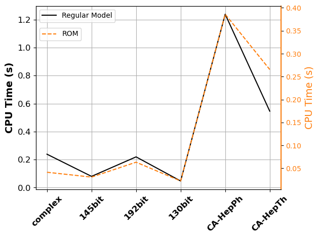
Time taken to evaluate vector field $f$ Equation (9) of regular model vs ROM vector field, see Equation ($f2$).

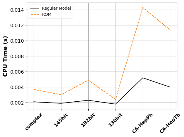
Execution time for $A^{T}_{s}x_{s}$ in ROM and full model with a random vector $x_{s}$.(see Section 8)

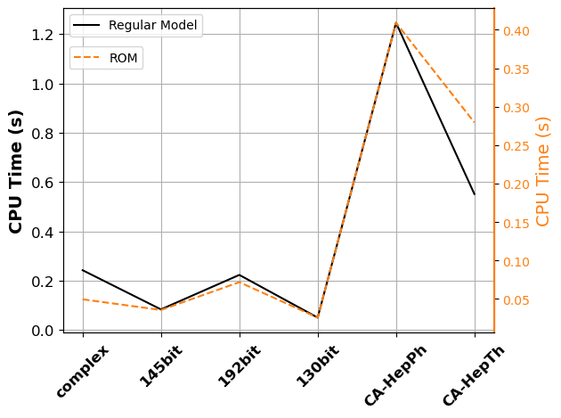
Time taken for ROM versus regular model.

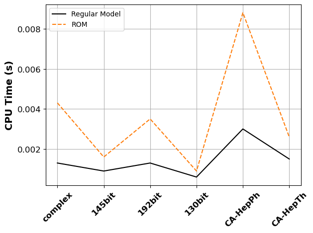
Execution time for $B^{T}_{j}y_{j}$ in ROM and full model with a random vector $y_{j}$.(see Section 8)

Figure 2: Impact of model reduction techniques for some real world graphs

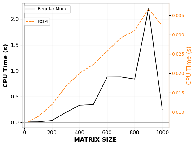
Time taken to evaluate vector field $f$ Equation 9 of regular model vs ROM vector field, see Equation ($f2$).

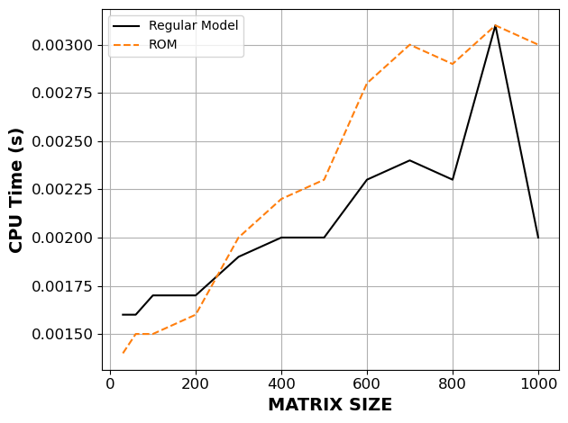
Execution time for $A^{T}_{s}x_{s}$ in ROM and full model with a random vector $x_{s}$.(see Section 8)

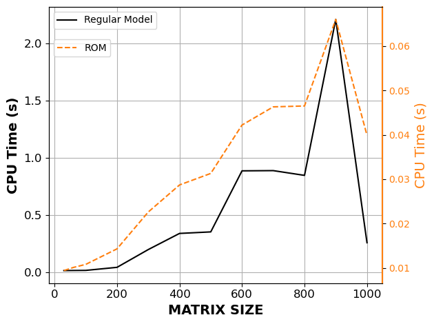
Time taken for ROM versus regular model.

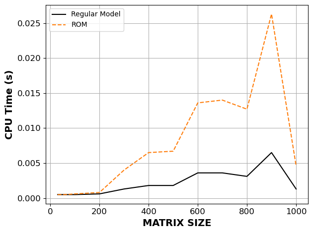
Execution time for $B^{T}_{j}y_{j}$ in ROM and full model with a random vector $y$.(see Section 8)

Figure 3: Impact of model reduction techniques for random graphs

5 Problem statement

Considering a subset of trajectories of a complex system on an undirected graph, the objective is to create an edge sparsifier (i.e. graphs with fewer edges than the original graph), and the sparse graph should produce patterns similar to the given subset of trajectories. This problem is posed as a constrained optimization problem where the objective function is made to include a term involving the difference between the observations from the given trajectories projected into a reduced dimension at various time points and the state vectors generated by the reduced order forward model based on the sparsified graph. An $\ell_{1}$ norm term of the weight multipliers ($\bar{\gamma}$) (Section 2.2) is also introduced as a penalty term in the objective function to induce sparsity.

The new weight vector $\bar{w}=\textrm{diag($w$)}\bar{\gamma}$. We denote the perturbed Laplacian matrix $L^{{}^{\prime}}=L+B^{T}DB,$ where $D=\text{diag(}\bar{w}-w)$. When this perturbed Laplacian matrix has many eigenmodes similar to the eigenmodes of the original network, the resulting patterns in the new graph will be highly correlated with the patterns in the original network. Thus any patterns or behaviours induced in the original network will likely be present in the new graph, see [12]. Computation of eigenmodes of the Laplacian matrix can be computationally intensive, so we propose approximations to determine the eigenmodes of the Laplacian matrix under perturbations, see Section 5.1.2.

5.1 Ensuring isodynamic behaviour

This section discusses techniques to ensure isodynamic behaviour on the sparse graph and the challenges involved. The dispersion relation connects the stability of the system as described by Equation (1) with the Laplacian matrix eigenvalues. A graph with no unstable mode will have (Re$(\lambda)<0)\,\forall\,\alpha$. The contribution of the $\alpha$-th eigenvalue to the stability of the system is given by the eigenvalues of the following matrix,

$$J_{\alpha}=D_{r}\mathcal{F}(r^{\star})-\left[\begin{array}[]{cc}D_{x}&0\\ 0&D_{y}\end{array}\right]\lambda{\;}^{(\alpha)}\;$$

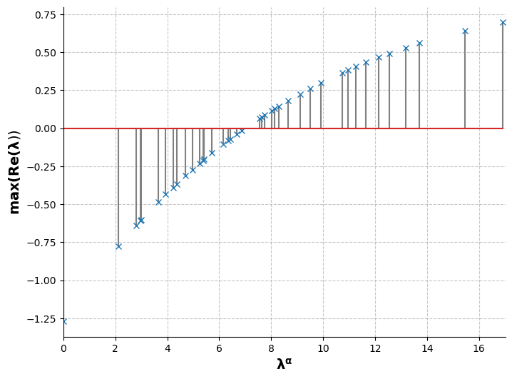
Figure 4: Plot showing the stable and unstable eigenmodes of reaction-diffusion system as described by Equation (1) on an Erdős-R$\acute{e}$nyi random graph

Figure 4 indicates the stable and unstable eigenmodes of a reaction-diffusion system (Eq. 1) cast on a random graph. The study in [12] aims at producing a pattern invariant network using techniques like eigenmode randomization and local rewiring. One could use the error function employed in the local rewiring methodology as mentioned in [12] as a constraint to the optimization problem discussed in Section 6 but computing this function iteratively can become computationally expensive. The error function imposed as a constraint will be generally non-smooth. Methods to approach such non-smooth optimization problems using global optimization algorithms like Genetic algorithms are discussed in [30], however mutliple function evaluations can make these methods ineffective. The error function ($\zeta$) introduced below is a modified variant of the one described in [12].

$$\zeta=n\zeta_{l}+\zeta_{q}$$

$$\zeta_{l}=\frac{\sum_{i=1}^{n_{p}}|\tilde{\lambda}_{i}-\lambda_{i}|^{2}}{n_{p}\;\;\sum_{i=1}^{n_{p}}(\lambda_{i})^{2}}$$

$$\zeta_{q}=\frac{\sum_{i=1}^{n_{p}}|\langle\tilde{\phi}_{i},\phi_{i}\rangle-1|^{2}}{n_{p}}$$

Here $n_{p}$ denotes the number of eigenmodes preserved; we accept the new graph if the error function $\zeta$ is less than a tolerance value.

In the presence of a connected input graph, we impose a minimum connectivity constraint to minimize the number of disconnected components, which, in turn, affects the error function (see Section 5.1). The intuition is taken from work in [21] which states that when the sum of two lowest degrees of the graph component can influence the second smallest eigenvalue of the Laplacian matrix. We control the sum of degrees of the graph by ensuring that the unsigned incidence matrix times the weight vector is greater than a required connectivity level, say $\tau\mathbf{1}_{n\times 1}$ with $\tau$ being a user-defined parameter. We demonstrate this using an example, see Figure 5.

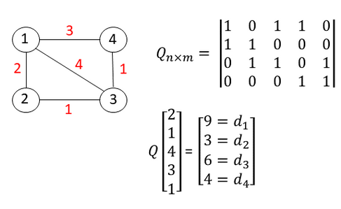
Figure 5: Figure illustrating on how the connectivity constraint is imposed using the unsigned incidence matrix. We consider an unweighted graph having 4 nodes and the multipliers are denoted by red. Here $Q$ denotes the unsigned incidence matrix, weight vector $w$ = diag($\mathbf{1}_{5\times 1})\gamma$, where $\gamma$ are the multipliers denoted by red. Degree vector $d=Q\gamma$.

5.1.1 Eigenvalue and eigenvector computation for the Laplacian matrix under perturbations

Lemma 5.1.

(Sherman-Morrison formula). If A is a singular $n\times n$ matrix and x is a vector, then

$$(A+xx^{T})^{-1}=A^{-1}-\frac{A^{-1}xx^{T}A^{-1}}{1+x^{T}A^{-1}x}.$$

Lemma 5.2.

(matrix determinant lemma) If A is nonsingular and x is a vector, then

$$\text{det}(A+xx^{T})=\text{det}(A)(1+x^{T}A^{-1}x).$$

We present the challenges in finding the eigenpair during each iteration of the optimization procedure. If there is a change to only one of the edges of the graph, then one could use the approximate model described as in [4] making use of Lemma 5.1 and 5.2 to find the eigenpairs. At iteration $q$ of the algorithm, we will get a new graph with the weights modified according to the scale factor $\bar{\gamma}^{q}$. We define the matrix $D=\text{diag(}\bar{\gamma}^{q}-\mathbf{1}_{m\times 1}$) and $\tilde{\lambda}=\mathrm{diag(}\lambda_{1},\lambda_{2},\lambda_{3},..,\lambda_{n})$ denotes the eigenvalues of matrix $L$. We define the new Laplacian matrix as $L^{{}^{\prime}}=L+B^{T}W^{1/2}DW^{1/2}B.$ The characteristic polynomial of matrix $L^{{}^{\prime}}$ is given by,

$$\chi_{L^{{}^{\prime}}}(\lambda,D)=\mathrm{det(}L^{{}^{\prime}}-\lambda I)=\mathrm{det(}\Phi\,\tilde{\lambda}\,\Phi^{T}+B^{T}W^{1/2}DW^{1/2}B-\lambda I)\;$$

Using the property of determinants we get the following

$$\chi_{L^{{}^{\prime}}}(\lambda,D)=\text{det(}\Sigma+U^{T}DU)\,\,\text{where}\,\,U^{T}=\Phi^{T}B^{T}W^{1/2}$$

$$\Sigma=diag(1,\lambda_{2}-\lambda,....,\lambda_{n}-\lambda)$$

$$\begin{array}[]{l}\text{ $\chi_{L^{{}^{\prime}}}(\lambda$, $D$) = det}\left[\begin{array}[]{cccc}1&0&\ldotp&0\\ 0&u_{2}^{T}Du_{2}+\lambda_{2}-\lambda&\ldotp&u_{2}^{T}Du_{n}\\ \ldotp&u_{3}^{T}Du_{2}&\ldotp&u_{3}^{T}Du_{n}\\ \ldotp&\ldotp&\ldotp&\ldotp\\ 0&u_{n}^{T}Du_{2}&\ldotp&u_{n}^{T}Du_{n}+\lambda_{n}-\lambda\end{array}\right]\\ \\ \text{$\chi_{L^{{}^{\prime}}}(\lambda$, $D$) = det }\bigg{(}\left[\begin{array}[]{ccc}\mathrm{trace}\left(u_{2}{\;u}_{2}^{T}\;D\right)+\lambda_{2}-\lambda&\ldotp&\ldotp\\ \mathrm{trace}\left(u_{3}\;u_{2}^{T}\;D\right)&\ldotp&\ldotp\\ \ldotp&\ldotp&\ldotp\\ \mathrm{trace}\left(u_{n}u_{2}^{T}\;D\right)&\ldotp&\ldotp\end{array}\right]\bigg{)}\end{array}$$

Finding the determinant of matrices with symbolic variables is described in [20]. We need to precompute only the diagonal elements of $u_{i}u^{T}_{j}$ to obtain the expression for the characteristic polynomial since $D$ is a diagonal matrix. Finding all the roots of the polynomial at each iteration and filtering out the highest roots may be more computationally expensive than finding only extreme eigenvalues as in ([25], [43]).

Example:

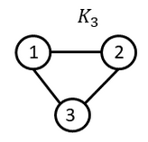
Figure 6: Complete graph $\mathbb{K}_{3}$

Let us consider the case of a complete graph on 3 vertices $\mathbb{K}_{3}$ Figure 6. The Laplacian matrix of this graph is given by

$$\;\;\;L=\begin{bmatrix}2&-1&-1\\ -1&2&-1\\ -1&-1&2\\ \end{bmatrix}$$

The eigenvalues of the matrix $L$ are $\lambda_{1}=0,\lambda_{2}=3,\lambda_{3}=3.$ Now let us perturb two of the weights of this graph and let the multiplier vector $\bar{\gamma}=[1.2,1.4,1]$. The matrix $D=\mathrm{diag(\bar{\gamma}}-\mathbf{1}_{3\times 1}).$ The matrix $B^{T}$ is given as follows,

$$\;\;\;B^{T}=\begin{bmatrix}1&0&-1\\ -1&1&0\\ 0&-1&1\\ \end{bmatrix}$$

The expression given by Equation (5.1.1) will then become $p(\lambda)=\mathrm{det(}\begin{bmatrix}3.9374-\lambda&-0.0786\\ -0.0786&3.2626-\lambda\end{bmatrix})$. $p(\lambda)=\lambda^{2}-7.2\lambda+12.84.$ The roots of the polynomial $p$ are given by 3.2536 and 3.9464, which are the eigenvalues of the matrix $L^{{}^{\prime}}$.
The effect on eigenvalues of a matrix with a perturbation is studied in [7]. One such significant result in the field of perturbation theory is given below.

Theorem 5.3.

([7]) If A and A + E are $n\times n$ symmetric matrices, then

$$|\lambda_{k}(A+E)-\lambda_{k}(A)|\leq||E||_{2}$$

for $k=1:n$

The aforementioned result can be employed to approximate the eigenvalue term in the error function ($\zeta_{l}$) described in Section 5.1. However, we currently lack a bound for the $\zeta_{q}$ term, and computing the $\ell_{2}$ norm of the matrix involves finding the largest eigenvalue, which is computationally expensive.
We propose an approximation for the eigenvalue and the eigenvector for the new Laplacian matrix based on the eigenvalues and eigenvectors of the original Laplacian matrix making use of the method of Rayleigh iteration, which produces an eigenvalue, eigenvector pair.
Rayleigh Iteration: $A\in\mathbb{R}^{n\times n}$ symmetric
$x_{0}$ given, $||x_{0}||_{2}=1$

  for $i=0,1$ to … do

     $\mu_{k}=r(x_{k})$   $(r(x)=\frac{x^{T}Ax}{x^{T}x})$

     Solve ($A$ - $\mu_{k}\mathbb{I})z_{k+1}=x_{k}$ for $z_{k+1}$

     $x_{k+1}=z_{k+1}/||z_{k+1}||_{2}$

  end for

5.1.2 Approximations to eigenpair

The Rayleigh quotient iteration algorithm is a powerful tool for computing eigenvectors and eigenvalues of symmetric or Hermitian matrices. It has the property of cubical convergence, but this only holds when the initial vector is chosen to be sufficiently close to one of the eigenvectors of the matrix being analyzed. In other words, the algorithm will converge very quickly if the initial vector is chosen carefully. From the first step in Rayleigh iteration we get $\mu_{0}=\lambda_{i}+\epsilon$, if we consider the $i$-th eigenvector $\phi_{i}$ as the initial point $x_{0}$. The next step requires solving for $z_{1}$ in the linear system $(A+E-\mu_{0}I)z_{1}=x_{0}$. Conducting the sensitivity of the linear system with a singularity is difficult to determine and is not trivial. The solution to the system $(A-\mu_{0}I)z=\phi_{i}$ is given by $-\frac{\phi_{i}}{\epsilon}$. The first iterate using the conjugate gradient method would then be given by $y_{i}=\frac{1}{\epsilon\;}\;\left(\frac{a^{T}a\;\;E\phi_{i}}{a^{T}\left(A+E-\lambda_{i\;}I\;-\epsilon I\;\right)a\;\;}-\phi_{i\;}\right)$. We consider this iterate as our eigenvector approximation after normalizing. The proposed approximations to the eigenpair are given below,

$$(\hat{\lambda}_{i},\hat{x}_{i})=\bigg{(}r(y_{i}),\frac{y_{i}}{||y_{i}||}\bigg{)}$$

In the following theorem, we propose bounds on the approximations of the proposed eigenpair.

Theorem 5.4.

Let $G$ be an undirected graph with Laplacian matrix $L$ and $L^{{}^{\prime}}=L+E$ be the perturbed Laplacian matrix, where $E=B^{T}DB$ represents the perturbations in the Laplacian matrix. We denote the $i$-th eigenvector estimate as $\hat{x}_{i}=\frac{y_{i}}{||y_{i}||_{2}}$, $y_{i}=\frac{1}{\epsilon\;}\;\left(\frac{a^{T}a\;\;E\phi_{i}}{a^{T}\left(A+E-\lambda_{i\;}I\;-\epsilon I\;\right)a\;\;}-\phi_{i\;}\right)$. Then $||(L+E-r(y_{i})I\,)\hat{x}_{i}||_{2}\leq\tau+||E||_{2}$, $\epsilon=\phi_{i}^{T}E\phi_{i}.$ Where $a=E\phi_{i}$, $\tau=max(|\lambda_{n}-\lambda_{2}(L+E)|,\lambda_{n}(L+E))$. $\lambda_{n}\geq\lambda_{n-1}\geq...\geq\lambda_{2}\geq\lambda_{1}$ denotes the eigen values of the Laplacian matrix of graph $G$.

Proof.

$||((L+E)-\frac{y_{i}^{T}(L+E)y_{i}}{y_{i}^{T}y_{i}}I)\hat{x}_{i}||=||(\Phi\Lambda\Phi^{T}-\frac{y_{i}^{T}(L+E)y_{i}}{y_{i}^{T}y_{i}}I+E)\hat{x}_{i}||$ (since Laplacian matrix is diagonalizable and $L=\Phi\Lambda\Phi^{T}$).

$$||(\Phi\Lambda\Phi^{T}-\frac{y_{i}^{T}(L+E)y_{i}}{y_{i}^{T}y_{i}}I+E)\hat{x}_{i}||\leq$$

$$||\Phi(\Lambda-\frac{y_{i}^{T}(L+E)y_{i}}{y_{i}^{T}y_{i}}I)\Phi^{T}+E||\,\,||\hat{x}_{i}||=||\Phi(\Lambda-\frac{y_{i}^{T}(L+E)y_{i}}{y_{i}^{T}y_{i}}I)\Phi^{T}+E||$$

Using the triangular inequality of matrix norms, the above inequality becomes

$$\leq||\Phi(\Lambda-\frac{y_{i}^{T}(L+E)y_{i}}{y_{i}^{T}y_{i}}I)\Phi^{T}||+||E||\leq\tau+||E||$$

It can be observed that $\mathbf{1}^{T}y_{i}=0$ and from the definition, we have $\lambda_{k}(L)=\mathrm{inf_{x\perp P_{k-1}}\,}\frac{x^{T}Lx}{x^{T}x}$ where $P_{k-1}$ is the subspace generated by eigenvectors of the Laplacian matrix $L$ given by
$\mathrm{span(}v_{1},v_{2},...,v_{k-1}).$ Thus the Fielder value or the second smallest eigenvalue $\lambda_{2}$ of the Laplacian matrix is given by $\lambda_{2}=\mathrm{inf_{x\perp\mathrm{1}}}\frac{x^{T}Lx}{x^{T}x}$ and the largest eigenvalue $\lambda_{n}=\text{sup}_{x}\frac{x^{T}Lx}{x^{T}x}$. Thus the above inequality becomes

$$\leq\tau+||E||\mathrm{\,\,,where\,\,\tau=max(|\lambda_{n}-\lambda_{2}(\textit{L+E})|,\lambda_{n}(\textit{L+E}))}$$

∎

The error function using the estimate would then be

$$\boxed{\bar{\zeta}=n\frac{\sum_{i=1}^{n_{p}}|\hat{\lambda}_{i}-\lambda_{i}|^{2}}{n_{p}\;\;\sum_{i=1}^{n_{p}}(\lambda_{i})^{2}}+\frac{\sum_{i=1}^{n_{p}}|\langle\hat{x}_{i},\phi_{i}\rangle-1|^{2}}{n_{p}}}$$

From ([37]), the following definition apply to pseudo spectra of matrices.
If $A$ is an $N\times N$ matrix and for $\lambda$ to be an $\epsilon-$pseudo-eigenvalue of A is

$$\sigma_{N}(\lambda I-A)\leq\epsilon$$

where $\sigma_{N}$ denotes the smallest singular value. From the above definition, we can see that our estimate $\hat{\lambda}_{i}$ is a $\tau+||E||_{2}$-pseudo eigenvalue of L.
We modify the constraint $\zeta\leq\beta_{1}$ by $\bar{\zeta}\leq k_{1}\beta_{1}$, where $k_{1}$ and $\beta_{1}$ are user defined constants.
We present numerical experiments on certain graphs, and for every graph, we take the number of eigenmodes to preserve as the largest eigenmodes of the Laplacian matrix of the graph. Random perturbation is given to every edge of the graph, and a comparison is between $\zeta$ and $\bar{\zeta}$ (Table 1).

Figures showing the effectiveness of the approximate eigenpair in preserving the eigenvalues and eigenvectors are described by Figures in Section 2.

Theorem 5.5.

Given an undirected graph $G=(V,E,W)$, with the Laplacian matrix $L$, then the matrix $M=L-(pI)$ is not orthogonal $\forall\,p\in\mathbb{R}$ if the minimum degree of the graph $d_{\mathrm{min}}(G)>2.$

Proof.

We prove the above theorem by contradiction. For a matrix $M$ to be orthogonal, we require $M^{T}M=I$. The eigenvalue decomposition of the matrix $L=\Phi\Lambda\Phi^{T}$. Applying the definition of the orthogonality of matrices to the matrix $M$, we get $\Phi(\Lambda-pI)^{2}\Phi^{T}=I$. Using the property of similarity of matrices, we can observe that all the eigenvalues of $\Phi(\Lambda-pI)^{2}\Phi^{T}$ should be 1. From the zero eigenvalue of the matrix $L$, $p=\pm 1$. The remaining eigenvalues of the Laplacian matrix should be either 0 or 2 according to this $p$ value, but since the minimum degree of the graph is greater than 2, this cannot be the case as the largest eigenvalue of the Laplacian matrix of the graph will be greater than or equal to the minimum degree ($\lambda_{n}\geq d_{\text{min}}>2,\;\lambda_{n}=\text{sup}_{x}\frac{x^{T}Lx}{x^{T}x}$, taking $x=e_{1}$, where $e_{i}$ denotes the canonical vector with a 1 in the $i$th coordinate and $0^{\prime}$s elsewhere). ∎

We make use of Theorem 5.5 in the section below (see Eq. 5.1).

Points of discontinuity for the function $\bar{\zeta}$

Discontinuities in $\bar{\zeta}$ can happen due to the following cases,
Case 1:

$$\phi_{i}^{T}E\phi_{i}=0.$$

Case 2:

$$a^{T}(L+E-\lambda_{i}I-\epsilon I)a=0,\text{\;where\;}a=E\phi_{i}\neq\mathbf{0}_{n\times 1}.$$

Considering the first case, one possibility is when $E$ is a rotation matrix. However matrix $E$ is not orthogonal $(\text{det}(E)=0)$. The other possibility is when $\phi_{i}\,\in$ nullspace($E$). If this happens, then we could see that $(\lambda_{i},\phi_{i})$ is an eigenvalue, eigenvector pair for the new Laplacian matrix. Possible candidates of $\gamma$ satisfying this condition are given by the solution to the under-determined linear system under non-negativity constraints.

$$R\gamma=\lambda_{i}\phi_{i},\,\mathrm{where\,\,}R=B^{T}W^{1/2}\text{$\text{diag}(W^{1/2}B\phi_{i})$}$$

$$\gamma\geq 0$$

Case 2 occurs when $a\neq\mathbf{0}_{n\times 1}\,\text{and}\,a^{T}(\tilde{L}-(\lambda_{i}+\phi_{i}^{T}E\phi_{i})I)a=0.$ One possibility is that $M_{i}=(\tilde{L}-(\lambda_{i}+\phi_{i}^{T}E\phi_{i})I)$ needs to be a rotation matrix, but this case cannot happen if we impose a minimum degree constraint as mentioned in Theorem 5.5. Elements in the nullspace of matrix $M_{i}$ under non-negativity constraints are candidates for discontinuity of the function $\bar{\zeta}$. We modify the eigenpair based on the following discontinuities.

$$(\tilde{\lambda}_{i},\tilde{\phi}_{i})=\begin{cases}(\lambda_{i},\phi_{i}),\hskip 85.35826pt\text{if }E\phi_{i}=\mathbf{0}_{n\times 1}\\ (\frac{a^{T}M_{i}a}{a^{T}a},\phi_{i}),\hskip 68.2866pt\text{if }y_{i}=\mathbf{0}_{n\times 1}\text{\;and\;}\\ \hskip 147.95433ptE\phi_{i}\neq\mathbf{0}_{n\times 1}\\ (\lambda_{i}+\phi_{i}^{T}E\phi_{i},\frac{a}{||a||}),\hskip 42.67912pt\text{if }M_{i}a=\mathbf{0}_{n\times 1},\\ \hskip 128.0374pty_{i},E\phi_{i}\neq\mathbf{0}_{n\times 1}\\ \hskip 128.0374pt\text{\; and \;}||y_{i}||<\infty\\ (\hat{\lambda}_{i},\hat{x}_{i}),\hskip 85.35826pt\text{otherwise}\end{cases}$$

The error function now is modified as

$$\bar{\zeta}(\bar{\gamma})=\frac{n}{n_{p}\sum_{i=1}^{n_{p}}(\lambda^{i})^{2}}\sum_{i=1}^{n_{p}}(\tilde{\lambda}_{i}-\lambda_{i})^{2}+\frac{1}{n_{p}}\sum_{i=1}^{n_{p}}(\langle\tilde{\phi_{i}},\phi_{i}\rangle-1)^{2}.$$

The summation terms could be computed in parallel using multiple cores of the machine for large graphs. The speedup obtained when evaluating this function in parallel is shown in Table 1 and Figure 8.

Gradient of error function $\bar{\zeta}$

$$\frac{d\bar{\zeta}}{d\gamma}=\frac{2n}{n_{p}\sum_{i=1}^{n_{p}}(\lambda^{i})^{2}}\sum_{i=1}^{n_{p}}(\tilde{\lambda}_{i}-\lambda_{i})\frac{d\tilde{\lambda}_{i}}{d\bar{\gamma}}+\frac{2}{n_{p}}\sum_{i=1}^{n_{p}}(\langle\tilde{\phi}_{i},\phi_{i}\rangle-1)\hskip 5.69054pt(D_{\bar{\gamma}}\tilde{\phi}_{i})^{T}\phi_{i}$$

$$\hat{\lambda}_{i}=\frac{y(\bar{\gamma})^{T}\tilde{L}y(\bar{\gamma})}{y(\bar{\gamma})^{T}y(\bar{\gamma})}$$

$$\frac{d\hat{\lambda}_{i}}{d\bar{\gamma}}=\frac{y(\bar{\gamma})^{T}y(\bar{\gamma})\hskip 5.69054pt\nabla{y(\bar{\gamma})^{T}\tilde{L}y(\bar{\gamma})}-(y(\bar{\gamma})^{T}\tilde{L}y(\bar{\gamma}))\;\nabla{y(\bar{\gamma})^{T}y(\bar{\gamma})}}{(y(\bar{\gamma})^{T}y(\bar{\gamma}))^{2}}$$

$$\nabla_{\bar{\gamma}}{y(\bar{\gamma})^{T}\tilde{L}y(\bar{\gamma})}=2D_{\bar{\gamma}}(B_{1}(\bar{\gamma}))^{T}B_{1}(\bar{\gamma})$$

$$B_{1}(\bar{\gamma})=\bar{\gamma}^{1/2}W^{1/2}By(\bar{\gamma})$$

$$\nabla{y(\bar{\gamma})^{T}y(\bar{\gamma})}=2(D_{\bar{\gamma}}y(\bar{\gamma}))^{T}y(\bar{\gamma})$$

$$\hat{x}_{i}=\frac{y(\bar{\gamma})}{||y(\bar{\gamma})||},\;\nabla\left(\frac{y_{j}(\bar{\gamma})}{||y||}\right)=\left(\frac{\nabla y_{j}(\bar{\gamma})}{||y||}-\frac{y_{j}(\bar{\gamma})\,D_{\bar{\gamma}}y(\bar{\gamma})^{T}y(\bar{\gamma})}{||y||^{3}}\right)$$

Graph	n	$n_{p}$	m	Relative error $\frac{(\zeta-\bar{\zeta})}{\zeta}$	speedup    (serial)	speedup   (parallel)
complex	1408	282	46326	0.0013	1.5532	0.9061
145bit	1002	201	11251	0.0122	3.2414	0.4946
192bit	2600	520	35880	0.0362	13.7567	11.9106
130bit	584	117	6058	0.0088	2.9379	0.1888
Ca-HepPh	11204	2241	117619	0.0079	27.4243	77.1951
Ca-HepTh	8638	1728	24806	0.0341	83.6472	184.8210

Table 1: Table showing comparison of $\zeta$ and $\bar{\zeta}$ for real world graphs with random perturbation to the edges.

6 Optimization problem

The sparsification framework we propose involves solving a constrained optimization problem, and the underlying constrained optimization problem is discussed in this section. In the optimization objective function (Eq. 10), we strive to promote sparsity in the multipliers by incorporating a term that involves the $\ell_{1}$ norm. Optimization using $\ell_{1}$ term generally induces sparsity. The term ($T_{1}$) in the objective function seeks to minimize the disparity between the observations at different time points, projected onto a reduced dimensional space derived from various trajectories, and the states obtained at these times using the reduced order model with the weights $\bar{w}=\text{diag($w$)}\bar{\bar{\gamma}}$. Here $F^{c}(t_{j})$ represents the observation from trajectory $c$ at time $t_{j}$. The initial conditions used to get observations $F^{c}(\cdot)$ will be kept invariant (Eq. 9.c2). $Q^{{}^{\prime}}=Q\,\text{diag($w$)}$, where $Q$ represents the unsigned incidence matrix of the graph (Figure 5), matrix $Q^{{}^{\prime}}$ is used to impose the connectivity constraint (Eq. 9.c3). $A^{c}$ contains indices of observations assimilation from trajectory c. $\bar{F}^{c}(\cdot)$ follows the forward model $M(\cdot)$, the discretization for the reduced order model (Eq. 9.c1). Constraint $\bar{\zeta}\leq k_{1}\beta_{1}$ tries to minimize perturbations to the largest $n_{p}$ eigenmodes of the Laplacian matrix (Eq. 9.c5).

$$\\ \\ \textbf{minimize}\,\,J(\bar{\gamma})=\underbrace{\frac{\sum_{c=1}^{\omega}\sum_{j\in A^{c}}||(F^{c}(t_{j})-\bar{F}^{c}(t_{j})\;)||^{2}}{2}}_{T_{1}}+\color[rgb]{0,0,1}{{\frac{\alpha}{2}\sum_{i=1}^{m}|\bar{\gamma}_{i}|}}$$ (10)

subject   to

$$\bar{\mathcal{F}}^{c}_{q+1}=M(\bar{\mathcal{F}}^{c}_{q},\bar{\gamma})\quad c=1,\dots,\omega,\;\;q=0,1,\dots,T-1,$$ (9.c1)

$$\bar{F}^{c}_{0}=F^{c}_{0}$$ (9.c2)

$$Q^{{}^{\prime}}\bar{\gamma}\geq\tau\quad$$ (9.c3)

$$\bar{\gamma}_{j}\geq 0, j=1,2,\dots,m$$ (9.c4)

$$\bar{\zeta}(\bar{\gamma})\leq k_{1}\,\beta_{1}$$ (9.c5)

The first variation of $J$ is given by

$$\vspace{-0.5mm}\delta J=\sum_{c=1}^{\omega}\sum_{j\in A_{c}}<(V_{j}^{c})^{T}\eta_{j}^{c},\delta\bar{\gamma}>+{\color[rgb]{0,0,1}\frac{\alpha}{2}<(\frac{|\bar{\gamma}_{1}|}{\bar{\gamma}_{1}},...,\frac{|\bar{\gamma}_{i}|}{\bar{\gamma}_{i}},..,\frac{|\bar{\gamma}_{n}|}{\bar{\gamma}_{n}}),\delta\bar{\gamma}>}\,\text{, see Equation (\ref{first_var})}$$

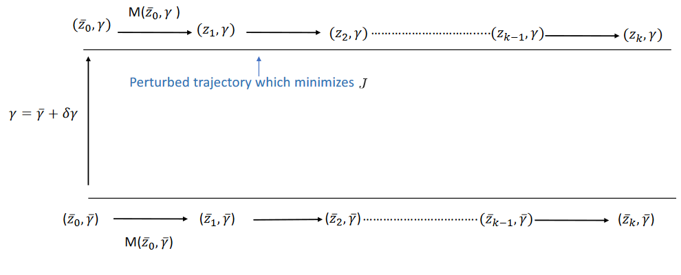
Figure 7: Data Assimilation approach.

The primary focus of our optimization routine is to minimize the function $J$ (Eq. (10)) subject to constraints. The gradient of $J$ is obtained using the adjoint method algorithm as mentioned in (Section 4.1.1). The model $M(\cdot)$ used for forward dynamics represents the discretization for the ROM to reduce computational complexity.

If we consider the optimization problem without the non-linear constraint, we can observe that the search space for our objective function described in (Eq. 10) can be made closed by using the substitution ($\bar{\gamma}=\gamma^{+}-\gamma^{-}$, $||\bar{\gamma}||_{1}=\mathbf{1}^{T}\gamma^{+}+\mathbf{1}^{T}\gamma^{-}$), where $\gamma^{+}$ represents the positive entries in $\gamma$, 0 elsewhere and $\gamma^{-}$ represents the negative entries in $\gamma$ and 0 elsewhere. So the objective function and the constraints are continuous. So we have an optimization problem as described below,

$$\min_{x\in X}f(x)\ \text{subject to\;}h_{j}(x)\leq 0,\;\;j=1,2,...n.$$

Set $X$ is closed where functions $f$ and $h_{j}$ are continuous. We could use the Barrier methods for optimization as described in ([30],[29]). The feasibility set $S=X\cap\{x\,|\,h_{j}(x)\leq 0\}$. If we generate a decreasing sequence $\epsilon_{k}$, let us denote $x_{k}$ as a solution to the problem $\mathrm{min_{x\in S}}\,\,f(x)+\epsilon_{k}B(x)$. Then every limit point of $\{x_{k}\}$ is a solution to the problem. One selection of barrier function $B(x)=-\sum_{j=1}^{n}\log(-h_{j}(x))$(Barrier convergence theorem). However, because of the discontinuities in the non-linear constraint, convergence in the constrained optimization problem may not be obtained. Heuristic algorithms for global optimization described in [30], like Genetic algorithms, Pattern search algorithms exist however require multiple function evaluations.

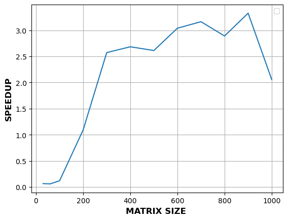
Figure 8: Speedup obtained for non-linear constraint evaluation.

Since the computation of the objective function in the optimization problem (Section 6) is computationally expensive, we do not prefer such methods.
ALGORITHM
  INPUT: $\displaystyle\text{An undirected Graph\;}G=(V,E,w)$ $\displaystyle\alpha-\;\ell_{1}\;\text{regularization parameter}$ $\displaystyle\tau_{|V|\times 1}-\text{connectivity parameter}$ $\displaystyle\epsilon-\text{edge pruning parameter}$ $\displaystyle N-\text{\;number of trajectories taken for POD step}$ $\displaystyle\omega-\text{number of trajectories taken for assimilation}$ $\displaystyle p_{1},p_{2},\dotsc,p_{\omega}-p_{i}\text{\;represents the number of points taken from trajectory $i$\;}\text{for assimilation}$ $\displaystyle k-\text{\;reduced dimension}$ $\displaystyle n_{p}-\text{number of eigenmodes taken for the non-linear constraint}$ $\displaystyle k_{1},\beta_{1}-\text{non-linear constraint parameters}$ $\displaystyle F^{1}_{0},F^{2}_{0},.....,F^{N}_{0}-\text{initial conditions for $N$ trajectories}$     OUTPUT: Sparse graph $\tilde{G}=(V,\tilde{E},\tilde{w})$          Procedure:   1. Run the forward reaction-diffusion model as in (Eq. 1) with initial conditions $F^{1}_{0},F^{2}_{0},.....,F^{N}_{0}$ and sample $p_{i}$ number of data points in the interval $[0,T]$, $i=1,2,\dotsc,\omega$ for assimilation, Sample data points at regular intervals for each trajectory thus obtaining the snapshot matrix containing $N$ trajectories.      2. From the snapshot matrix, obtain the matrix $\rho$ of projection and mean $\bar{x}$ as mentioned in (Section 4.3), selecting the $k$ largest eigenvectors of the covariance matrix.      3. From the $N$ trajectories, select $\omega\leq N$ trajectories for the data assimilation correction part.   4. Using the sampled trajectories, run the minimization procedure on the optimization problem discussed in (Section 6) to obtain the weight multipliers $\bar{\gamma}$.   5. On obtaining the multipliers, construct the weights $\bar{w}$ using the multiplier $\bar{\gamma}$, $\bar{w}=\text{diag($w$)}\bar{\gamma}$. Remove weights less than $\epsilon$ to obtain the new weights $w^{{}^{\prime}}$.   6. Construct $\tilde{G}$ using the weights $w^{{}^{\prime}}$. END ALGORITHM

Running time of the procedure

The time-consuming step in our sparsification procedure is solving a constrained non-linear programming problem (step 4 in algorithm). For every iteration of the optimization procedure, we need to compute the projected vector field (Eq. $f2$) which takes $O(k|V|^{2}$) operations. Evaluation of the gradient takes $O(k|E|)$ operations (Figure  9(a)).

The nonlinear constraint evaluation and the gradient evaluation take $O(|V|^{2}n_{p})$ and $O(|E|^{2}n_{p}$) operations (Figure 9(b)) respectively. Article [31] describes the challenges involved in solving a nonlinear constrained optimization problem. We exploit parallelism in the nonlinear constraint evaluation steps, and the speedups are shown in Figure 8.

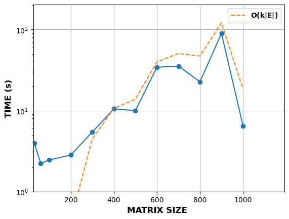
((a)) Figure showing the time complexity of cost function.

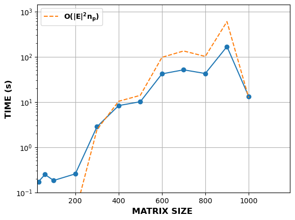
((b)) Figure showing time complexity of the non-linear constraint.

Figure 9: Time complexity

7 Results

The framework developed is applied to several real-world graphs ([38],[26]). The parameters in algorithm described in Section 6 were assigned as follows $\alpha=16\log(|E|)$, $p_{1},p_{2}$ = 50, $D_{x}=0.1$, $D_{y}=1.4$, $N=2$, $\omega=2$, $k_{1}=1$, $\beta_{1}=10^{-2}$, $\tau=\text{max(2.1,\,}0.1\,d_{\mathrm{min}})\mathbf{1}_{n\times 1}\,\,$, $\epsilon=10^{-2}$, $k=\mathrm{min(}\lceil\frac{n}{5}\rceil,50)$ and $n_{p}=\lceil n/5\rceil$, where $d_{\mathrm{min}}$ denotes the minimum degree of the graph. We include the $n_{p}$ largest eigenvalues and eigenvectors of the Laplacian matrix in the non-linear constraint evaluation step. The Euler forward method is used for finding the solution at discrete time steps in the adjoint sensitivity step, and the explicit Range-Kutta 4 slope method is used to generate snapshot matrices required for the POD step. The tabulated results on some real-world graphs are mentioned below (Table 2). The constrained optimization step is solved in MATLAB [17], and we are using the interior point method for constrained optimization as described in [31]. The correlation coefficient $R$ is obtained by comparing the grid of solution points of reaction-diffusion system (Eq. 1) on the original and sparsified graph for a random perturbation to the equilibrium point. We present an illustrative example of our frameworks performance on a 50-node Erdős-R$\acute{e}$nyi random graph, as depicted in Figure 10.

Figure 9 illustrates the comparison between the eigenpairs of the given graph and its corresponding sparsifier in Table 2.

Table 2:

complex

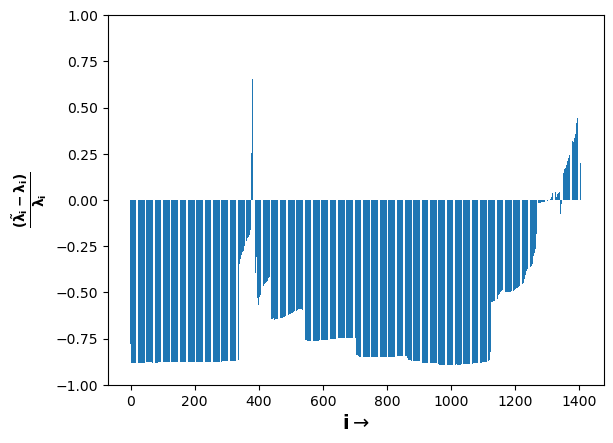
10.1(a)

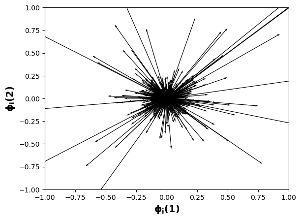
10.1(b)

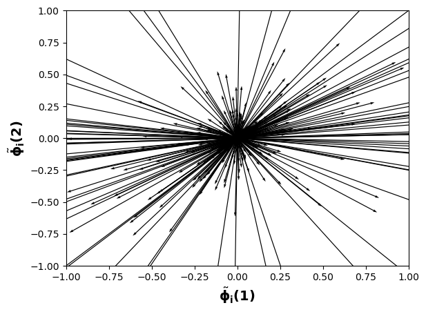
10.1(c)

130bit

10.2(a)

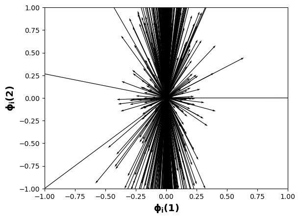
10.2(b)

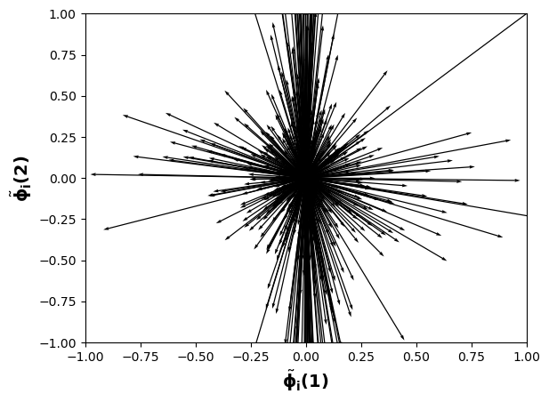
10.2(c)

145bit

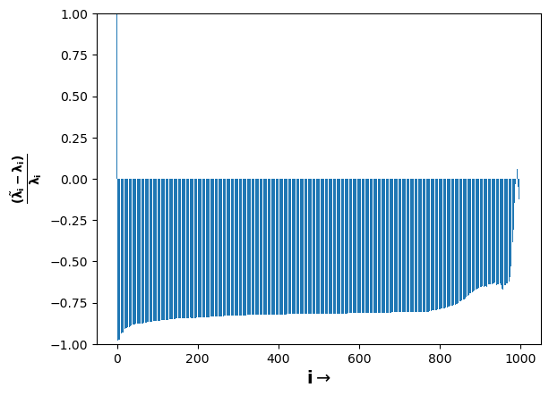
10.3(a)

10.3(b)

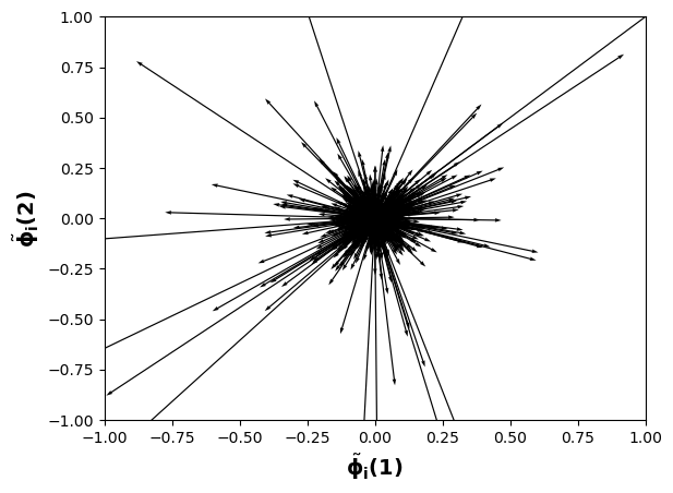
10.3(c)

192bit

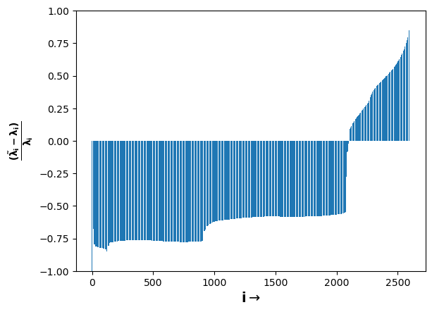
10.4(a)

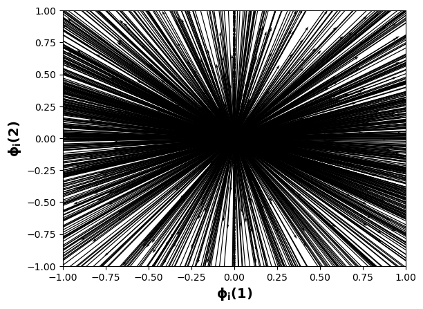
10.4(b)

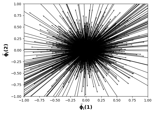
10.4(c)

CA-HepTh

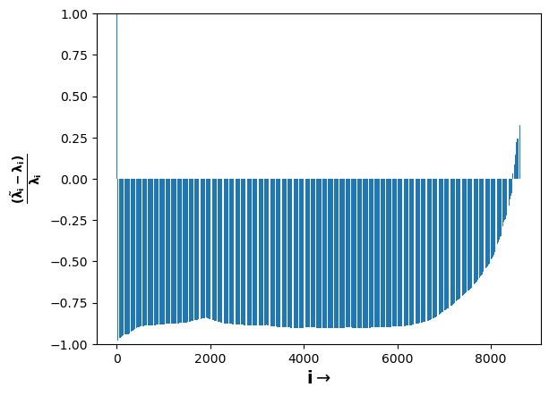
10.5(a)

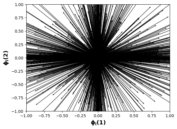
10.5(b)

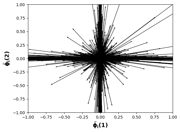
10.5(c)

Figure 9: Figures 10.(1-5)(a) shows the relative changes in the eigenvalues of the Laplacian matrix of the sparsifier($\frac{\tilde{\lambda}_{i}-\lambda_{i}}{\lambda_{i}}$). Figures 10.(1-5)(b) plot showing the first two coordinates of all the eigenvectors of the Laplacian matrix of the graph in the x and y-axis. Figures 10.(1-5)(c) plot showing the first two coordinates of all the eigenvectors of the Laplacian matrix of the sparsifier in the x and y-axis.

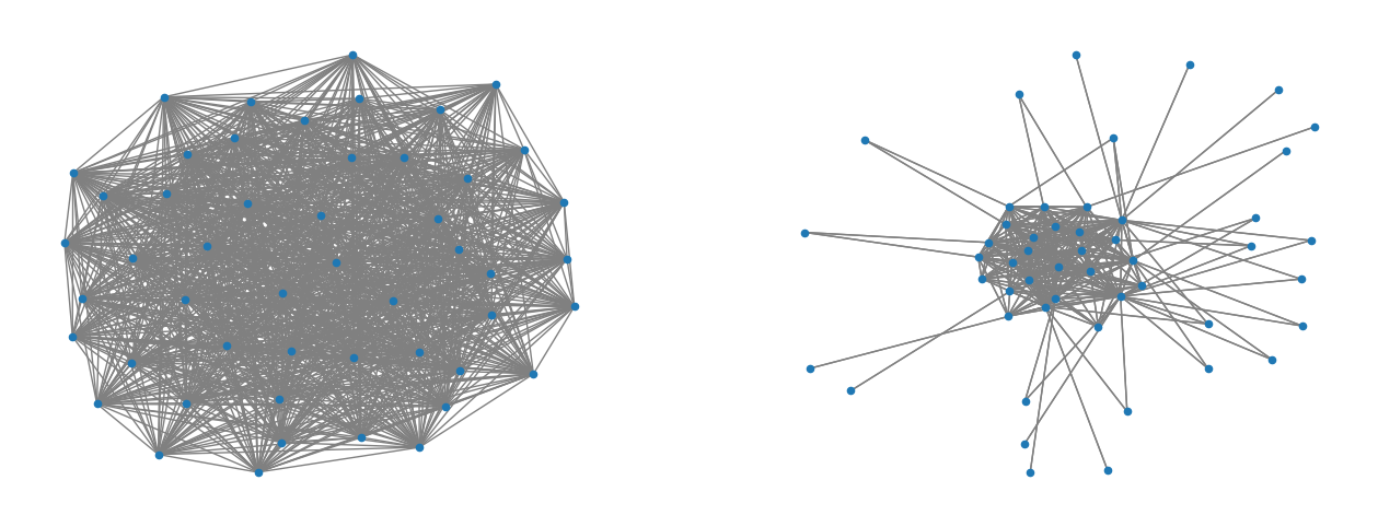
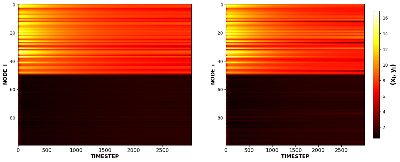
Figure 10: Figure showing patterns produced on an Erdős-R$\acute{e}$nyi 50 node random graph on the left and its sparsifier on the right.

8 Sparsifying ODENets

Neural ODEs or Neural Ordinary Differential Equations were first introduced by Chen et al. in their 2018 paper ”Neural Ordinary Differential Equations” [13]. The basic idea behind neural ODEs is to parameterize the derivative of the hidden state using a neural network. This allows the network to learn the system’s evolution over time rather than just mapping inputs to outputs. In other words, the neural network becomes a continuous function that can be integrated over time to generate predictions.

One of the key advantages of neural ODEs is that they can be used to model systems with complex dynamics, such as those found in physics, biology, and finance. They have been used for various applications, including image recognition, time series prediction, and generative modelling. This section looks at the possibility of our framework in sparsifying such ODENets. In this section, our focus lies in addressing the following question: Can we mimic the dynamics of a dynamical system on a neural ODENet with a collection of snapshots of solutions using a sparse set of parameters by leveraging the adjoint sensitivity framework within a reduced-dimensional setting?
Let us consider an example of a Linear dynamical system defined below.

$$\frac{dx}{dt}=Ax+b,\;\;A\in\mathbb{R}^{6\times 6},\;b\in\mathbb{R}^{6}.$$ (11)

For a predefined initial condition $x(0)=x_{0}$, the above problem will be an IVP. The neural network architecture proposed has one hidden layer with 50 neurons, with the input and output layers having six neurons for our experiment. A nonlinear activation is given at the output layer. The neural network output function proposed is given by

$$nn(x(t))=\sinh[\theta_{2}\theta_{1}x(t)+\theta_{2}b_{1}+b_{2}]$$

$$\text{\,\,}\theta_{1}\in\mathbb{R}^{50\times 6},\theta_{2}\in\mathbb{R}^{6\times 50},b_{1}\in\mathbb{R}^{50},b_{2}\in\mathbb{R}^{6}.$$

Procedure

1. Generate the projection matrix $\rho\in\mathbb{R}^{2\times 6}$ and mean $\bar{x}\in\mathbb{R}^{6}$ of projection based on the POD method (Section 4.3) using the snapshot matrix consisting of data points from the linear dynamical system (Eq. 11).

2. Sample $p$ data points without replacement from the snapshot matrix for assimilation, denoting this data as $\mathcal{D}=\{x_{i}\}_{i=1,2,\ldots,p}$. Using the projection matrix, project the data into reduced dimension ($\mathcal{D}_{\text{proj}}=\{\rho(x_{i}-\bar{x})\}_{i=1,2,\ldots,p}$). The projected neural network output function is given by,

   $$(nn_{\textbf{proj}}(z(t))=\rho\,\sinh[\theta_{2}\theta_{1}\rho^{T}z(t)+\theta_{2}\theta_{1}\bar{x}+\theta_{2}b_{1}+b_{2}]$$

3. For the sake of simplicity, we assume the parameters to be constant over time intervals. The adjoint sensitivity method for data assimilation is used to recover the parameters. The Euler forward method is used for the discretization of the projected neural ODE slope function. The cost function used for obtaining the parameters is given by (Eq. 10). For this experiment, we utilized a set of 10 observations obtained from a single trajectory, randomly selected from a pool of 500 timesteps. Additionally, the chosen regularization parameter $\alpha$ was set to 40.

   

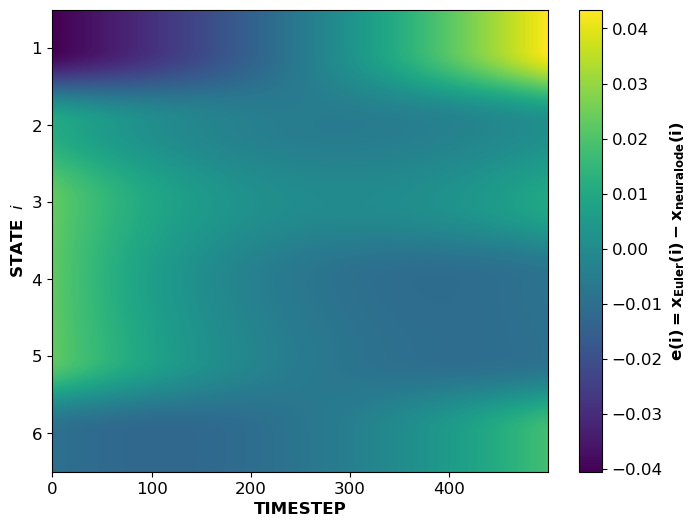
   Figure 11: Error in the solution obtained from neural ODENet compared with the Euler forward method on the linear dynamical system (Eq. 11).

   

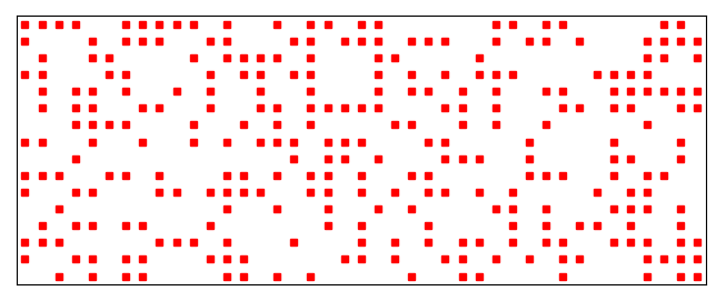
   Figure 12: Sparsity pattern in the parameter vector of the neural ODENet.

No constraints on the neural ODENet parameters are imposed, so the parameter estimation problem is unconstrained. The difference in the solutions obtained from the neural ODENet and the Euler forward step on the linear dynamical system described by Equation (11) is shown in the Figure 12. The number of non-sparse parameters obtained from step 3 is 289. The sparsity pattern of the parameters of the neural ODENet is shown in Figure 12.

9 Conclusion

We have developed a novel framework that enables efficient sparsification of undirected graphs through a dynamic optimization problem considering a subset of trajectories in a ROM space. The optimization objective focuses on preserving the patterns in a reduced dimension and giving importance to producing a sparse vector of weights. Our approach delivers good computational performance, with significantly high correlation coefficients obtained when comparing solutions for the sparse and original graphs under random perturbations. Table 1 compares the proposed approximations of the eigenpairs (Theorem 5.4) with the actual eigenpairs for several real-world graphs under random perturbations to the edges of the graph.

The adjoint method cost function on a ROM with an $\ell_{1}$ norm term produced a sparse vector of weight multipliers, as shown in Table 2, and the sparse network produced patterns similar to the given network. The framework proved to be also effective in sparsifying ODENets; the sparsity patterns are shown in Figure 12. To further improve our approach’s computational efficiency, we leveraged multi-core processing for evaluating the error function ($\bar{\zeta}$), resulting in significant speedup (Figure 8) when analyzing large graphs. Corrections done using observations in a ROM space proved to provide good computational performance; Figure 3 and Figure 2 demonstrate the performance of the POD method for the reaction-diffusion system (Eq. 1) on both random and real-world graphs.

The framework can be generalised to any reaction-diffusion systems involving undirected graphs. However, sparsifying and generating isodynamic patterns in the heterogeneous Kuramoto model as described in [22] and in other systems like the Ginzgurg-Landau model ([15]) involving directed graphs are out of scope for this work.

References

- [1] Kook Jin Ahn, Sudipto Guha, and Andrew McGregor. Graph sketches. Proceedings of the 31st symposium on Principles of Database Systems - PODS ’12, 2012.
- [2] Zeyuan Allen-Zhu, Zhenyu Liao, and Lorenzo Orecchia. Spectral sparsification and regret minimization beyond matrix multiplicative updates, 2015.
- [3] Y. Bard. Nonlinear parameter estimation. Academic Press, 1974.
- [4] Joshua Batson, Daniel A. Spielman, and Nikhil Srivastava. Twice-ramanujan sparsifiers. SIAM Review, 56(2):315–334, 2014.
- [5] András A. Benczúr and David R. Karger. Approximating s-t minimum cuts in Õ(n2) time. Proceedings of the twenty-eighth annual ACM symposium on Theory of computing - STOC ’96, 1996.
- [6] András A. Benczúr and David R. Karger. Randomized approximation schemes for cuts and flows in capacitated graphs. SIAM Journal on Computing, 44(2):290–319, 2015.
- [7] Rajendra Bhatia. Perturbation bounds for matrix eigenvalues. SIAM, 2007.
- [8] L. T. Biegler, J. J. Damiano, and G. E. Blau. Nonlinear parameter estimation: A case study comparison. AIChE Journal, 32(1):29–45, 1986.
- [9] Jenna A. Bilbrey, Kristina M. Herman, Henry Sprueill, Soritis S. Xantheas, Payel Das, Manuel Lopez Roldan, Mike Kraus, Hatem Helal, and Sutanay Choudhury. Reducing down(stream)time: Pretraining molecular gnns using heterogeneous ai accelerators, 2022.
- [10] Richard L. Burden, J. Douglas Faires, and Annette M. Burden. Numerical analysis. Cengage Learning, 2016.
- [11] Makis Caracotsios and Warren E. Stewart. Sensitivity analysis of initial value problems with mixed odes and algebraic equations. Computers and amp; Chemical Engineering, 9(4):359–365, 1985.
- [12] Giulia Cencetti, Pau Clusella, and Duccio Fanelli. Pattern invariance for reaction-diffusion systems on complex networks. Scientific Reports, 8(1), 2018.
- [13] Tian Qi Chen, Yulia Rubanova, Jesse Bettencourt, and David Duvenaud. Neural ordinary differential equations. CoRR, abs/1806.07366, 2018.
- [14] Wai Shing Fung and Nicholas J. A. Harvey. Graph sparsification by edge-connectivity and random spanning trees. CoRR, abs/1005.0265, 2010.
- [15] Vladimir García-Morales and Katharina Krischer. The complex ginzburg–landau equation: An introduction. Contemporary Physics, 53(2):79–95, 2012.
- [16] Navin Goyal, Luis Rademacher, and Santosh Vempala. Expanders via random spanning trees. Proceedings of the Twentieth Annual ACM-SIAM Symposium on Discrete Algorithms, 2009.
- [17] The MathWorks Inc. Matlab version: 9.13.0 (r2022b), 2022.
- [18] David R. Karger. Random sampling in cut, flow, and network design problems. Proceedings of the twenty-sixth annual ACM symposium on Theory of computing - STOC ’94, 1994.
- [19] David R. Karger. Random sampling in cut, flow, and network design problems. Mathematics of Operations Research, 24(2):383–413, 1999.
- [20] Tanya Khovanova and Ziv Scully. Efficient calculation of determinants of symbolic matrices with many variables, 2013.
- [21] Dinesh Kumar, Abhishek Ajayakumar, and Soumyendu Raha. Stability aware spatial cut of metapopulations ecological networks. Ecological Complexity, 47:100948, 2021.
- [22] Yoshiki Kuramoto. Chemical turbulence. Chemical Oscillations, Waves, and Turbulence, page 111–140, 1984.
- [23] S. Lakshmivarahan and J. M. Lewis. Forward sensitivity approach to dynamic data assimilation. Advances in Meteorology, 2010:1–12, 2010.
- [24] Kody Law, Andrew Stuart, and Konstantinos Zygalakis. Data assimilation: A mathematical introduction. Springer, 2015.
- [25] R. B. Lehoucq, D. C. Sorensen, and C. Yang. Arpack users’ guide. 1998.
- [26] Jure Leskovec and Andrej Krevl. SNAP Datasets: Stanford large network dataset collection. http://snap.stanford.edu/data, June 2014.
- [27] John M. Lewis, Sivaramakrishnan Lakshmivarahan, and Sudarshan Kumar Dhall. Dynamic Data Assimilation: A least squares approach. Cambridge Univ. Press, 2009.
- [28] Zichao Long, Yiping Lu, Xianzhong Ma, and Bin Dong. Pde-net: Learning pdes from data, 2017.
- [29] David G. Luenberger and Yinyu Ye. Linear and nonlinear programming. Springer, 2021.
- [30] Jorge Nocedal and Stephen J. Wright. Numerical optimization. Springer, 2006.
- [31] Jorge Nocedal, Figen Öztoprak, and Richard A. Waltz. An interior point method for nonlinear programming with infeasibility detection capabilities. Optimization Methods and Software, 29(4):837–854, 2014.
- [32] Ivo Nowak. Relaxation and decomposition methods for mixed integer nonlinear programming. International Series of Numerical Mathematics, 2005.
- [33] Cheryl C. Qu and Juergen Hahn. Process monitoring and parameter estimation via unscented kalman filtering. Journal of Loss Prevention in the Process Industries, 22(6):703–709, 2009.
- [34] Maziar Raissi and George Em Karniadakis. Hidden physics models: Machine learning of nonlinear partial differential equations. Journal of Computational Physics, 357:125–141, mar 2018.
- [35] Maziar Raissi, Paris Perdikaris, and George Em Karniadakis. Multistep neural networks for data-driven discovery of nonlinear dynamical systems, 2018.
- [36] Muruhan Rathinam and Linda R. Petzold. A new look at proper orthogonal decomposition. SIAM Journal on Numerical Analysis, 41(5):1893–1925, 2003.
- [37] Satish C. Reddy and Lloyd N. Trefethen. Lax-stability of fully discrete spectral methods via stability regions and pseudo-eigenvalues. Computer Methods in Applied Mechanics and Engineering, 80(1-3):147–164, 1990.
- [38] Ryan A. Rossi and Nesreen K. Ahmed. The network data repository with interactive graph analytics and visualization. In Proceedings of the Twenty-Ninth AAAI Conference on Artificial Intelligence, 2015.
- [39] Särkkä Simo. Bayesian filtering and smoothing. Cambridge Univ. Press, 2013.
- [40] Daniel A. Spielman and Nikhil Srivastava. Graph sparsification by effective resistances. Proceedings of the fortieth annual ACM symposium on Theory of computing, 2008.
- [41] Daniel A. Spielman and Shang-Hua Teng. Nearly-linear time algorithms for graph partitioning, graph sparsification, and solving linear systems. Proceedings of the thirty-sixth annual ACM symposium on Theory of computing - STOC ’04, 2004.
- [42] Daniel A. Spielman and Shang-Hua Teng. Spectral sparsification of graphs. SIAM Journal on Computing, 40(4):981–1025, 2011.
- [43] G. W. Stewart. A krylov–schur algorithm for large eigenproblems. SIAM Journal on Matrix Analysis and Applications, 23(3):601–614, 2002.
- [44] Guihong Wan and Haim Schweitzer. Edge sparsification for graphs via meta-learning. 2021 IEEE 37th International Conference on Data Engineering (ICDE), 2021.
- [45] Steffen Wiewel, Moritz Becher, and Nils Thuerey. Latent-space physics: Towards learning the temporal evolution of fluid flow, 2018.