Using Explanations to Guide Models

Abstract

Deep neural networks are highly performant, but might base their decision on spurious or background features that co-occur with certain classes, which can hurt generalization. To mitigate this issue, the usage of ‘model guidance’ has gained popularity recently: for this, models are guided to be “right for the right reasons” [42] by regularizing the models’ explanations to highlight the right features. Experimental validation of these approaches has thus far however been limited to relatively simple and / or synthetic datasets. To gain a better understanding of which model-guiding approaches actually transfer to more challenging real-world datasets, in this work we conduct an in-depth evaluation across various loss functions, attribution methods, models, and ‘guidance depths’ on the PASCAL VOC 2007 and MS COCO 2014 datasets, and show that model guidance can sometimes even improve model performance. In this context, we further propose a novel energy loss, show its effectiveness in directing the model to focus on object features. We also show that these gains can be achieved even with a small fraction (e.g. $1\%$) of bounding box annotations, highlighting the cost effectiveness of this approach. Lastly, we show that this approach can also improve generalization under distribution shifts. Code will be made available.

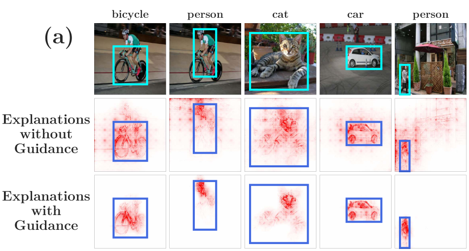
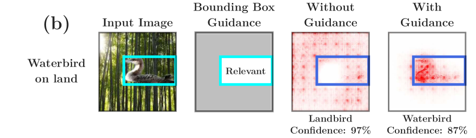
Fig. 1: (a) Model guidance increases object focus. Models may rely on irrelevant background features or spurious correlations (e.g. presence of person provides positive evidence for bicycle, center row, col. 1). Guiding the model via bounding box annotations can mitigate this and consistently increases the focus on object features (bottom row). (b) Model guidance can improve accuracy. In the presence of spurious correlations in the training data, non-guided models might focus on the wrong features. In the example image in (b), the waterbird is incorrectly classified to be a landbird due to the background (col. 3). Guiding the model via bounding box annotation (as shown in col. 2), the model can be guided to focus on the bird features for classification (col. 4).

1 Introduction

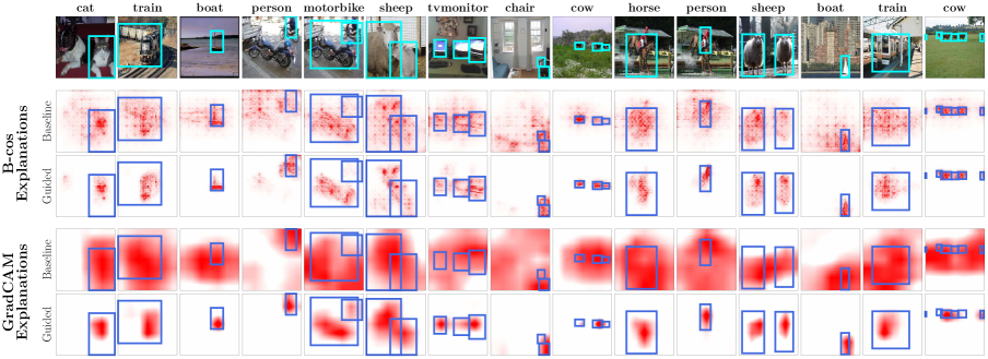
Fig. 2: Qualitative results of model guidance. We show model-inherent B-cos explanations (input layer) of a B-cos ResNet-50 and GradCAM explanations (final layer) of a conventional ResNet-50 before (‘Standard’) and after optimization (‘Guided’) for images from the VOC test set, using our proposed Energy loss (Eq. 6). Guiding the model via bounding box annotations consistently increases the focus on object features for both methods. Specifically, we find that background attributions are consistently suppressed in both cases.

Deep neural networks (DNNs) excel at learning predictive features that allow them to correctly classify a set of training images with ease. The features learnt on the training set, however, do not necessarily transfer to unseen images: e.g., instead of learning the actual class-relevant features, DNNs might memorize individual images (cf. [13]) or exploit spurious correlations in the training data (cf. [61]). For example, if bikes are highly correlated with people in the training data, a model might learn to associate the presence of a person in an image as positive evidence for a bike (e.g. Fig. 1a, col. 1, rows 1-2), which can limit how well it generalizes. Similarly, a bird classifier might rely on background features from the bird’s habitat, and fail to correctly classify in a different habitat (cf. Fig. 1b cols. 1-3 and [35]).

To detect and thus be able to correct such behaviour, recent advances in model interpretability have provided attribution methods (e.g. [46, 55, 50, 6]) as a means to understand a model’s reasoning. These methods typically provide attention maps that highlight regions of importance in an input to explain the model’s decisions. Consequently, they can be used to identify incorrect reasoning such as reliance on spurious or irrelevant features such as in Fig. 1b.

As many attribution methods are in fact themselves differentiable (e.g. [50, 55, 46, 6]), recent work [42, 49, 19, 18, 59, 57] has explored the idea of using them to guide the models to make them “right for the right reasons” [42]. Specifically, models can be guided by jointly optimizing for correct classification as well as for localization of attributions to human annotated masks. This can help the model focus on the relevant features of a class, and correct errors in reasoning (Fig. 1b, col. 4). Such guidance has the added benefit of providing well-localized masks that are easier to understand for end users (e.g. Fig. 2).

While model guidance has shown promising results, it has thus far been limited to simple and/or synthetic datasets, usually for binary classification tasks. Further, their evaluation is typically limited to specific attribution methods and localization optimization strategies, and they greatly vary in the types of datasets and human annotations used, which makes it difficult to compare them and understand if they translate to more challenging, real-world settings.

In this work, we perform an in-depth evaluation of model guidance on real-world, large scale datasets, and compare the effectiveness of a variety of attribution methods and localization losses. To reduce annotation cost, we only use coarse bounding box annotation masks over objects of each class in an image, and show that while existing approaches can localize to the masks, they often force the model to attribute background regions within the mask and worsen attribution granularity (cf. Fig. 7). To mitigate this, we propose a novel Energy localization loss, and show that it can be used with coarse annotations to guide models to focus only on the object itself (Fig. 1a, row 3).

Contributions. (1) We perform the first evaluation of model guidance on challenging large scale multi-label classification datasets (PASCAL VOC 2007 [12], MS COCO 2014 [28]), and compare across attribution methods, layers, and localization loss functions. Further, we show that, despite being relatively coarse, using bounding box supervision can provide sufficient guidance to the models while taking advantage of pre-existing annotations. (2) We propose a novel Energy loss for model guidance, and show its efficacy at localizing attributions to object features while avoiding irrelevant background features within the annotation masks. (3) We show that model guidance can be performed cost-effectively by using annotation masks that are noisy or are available for only a small fraction (e.g. $1\%$) of the training data. (4) We show through experiments on the Waterbirds-100 dataset [44, 35] that model guidance with a small number of annotations can help improve the model’s generalization under distribution shifts in the test data.

2 Related Work

Attribution Methods [51, 53, 55, 50, 46, 60, 10, 24, 8, 36, 15, 63, 40, 9, 4] are often used to explain black-box models by generating heatmaps that highlight input regions important to the model’s decision. However, such methods are often not faithful to the model [1, 39, 25, 65, 2] and risk misleading users. Recent work proposes inherently interpretable models [7, 6] that address this by providing model-faithful explanations by design. In our work, we use both popular post-hoc and model-inherent attribution methods to guide models and discuss their effectiveness.

Attribution Priors: Several approaches have been proposed for training better models by enforcing desirable properties on their attributions. These include enforcing consistency against augmentations [38, 37, 20], smoothness [11, 31, 26], separation of classes [64, 37, 54, 32, 52], or constraining the model’s attention [17, 3]. In contrast, in this work, we focus on providing explicit human guidance to the model using bounding box annotations. This constitutes more explicit guidance but allows fine-grained control over the model’s reasoning even with few annotations.

Model Guidance: In contrast to the indirect regularization effect achieved by attribution priors, approaches have also been proposed (cf. [16, 58]) to actively guide models using attributions as a tool, for a variety of tasks such as classification [42, 19, 18, 41, 35, 21, 56, 30, 59, 57, 45, 48, 29, 49, 62], segmentation [27], VQA [47, 56], and knowledge distillation [14]. The goal of such approaches is not only to improve performance, but also make sure that the model is “right for the right reasons” [42]. For classifiers, this typically involves jointly optimizing both for classification performance and localization to object features. However, most prior work evaluate on simple datasets [42, 48, 19, 18] or require modifying the network architecture [30, 29]. In this work, we conduct an in-depth evaluation and propose a novel loss function for guiding DNNs, and show its utility on much more challenging real-world multi-label classification datasets (PASCAL VOC 2007, MS COCO 2014). We also provide a comprehensive comparison against the localization losses introduced and used in the closest related work, i.e. RRR [42], HAICS [49], and GRADIA [19], and discuss their utility. Model guidance has also been used to mitigate reliance on spurious features using language guidance [35], and we show that using a small number of coarse bounding box annotations can be similarly effective.

Evaluating Model Guidance: The benefits of model guidance have typically been shown via improvements in classification performance (e.g. [42, 41]) or localization to the object mask (e.g. [18, 27]) by computing the IoU with the attribution maps. In addition to evaluating on these metrics as done in prior work, we also evaluate on the EPG metric [60], and use it to derive our energy loss.

3 Guiding Models Using Attributions

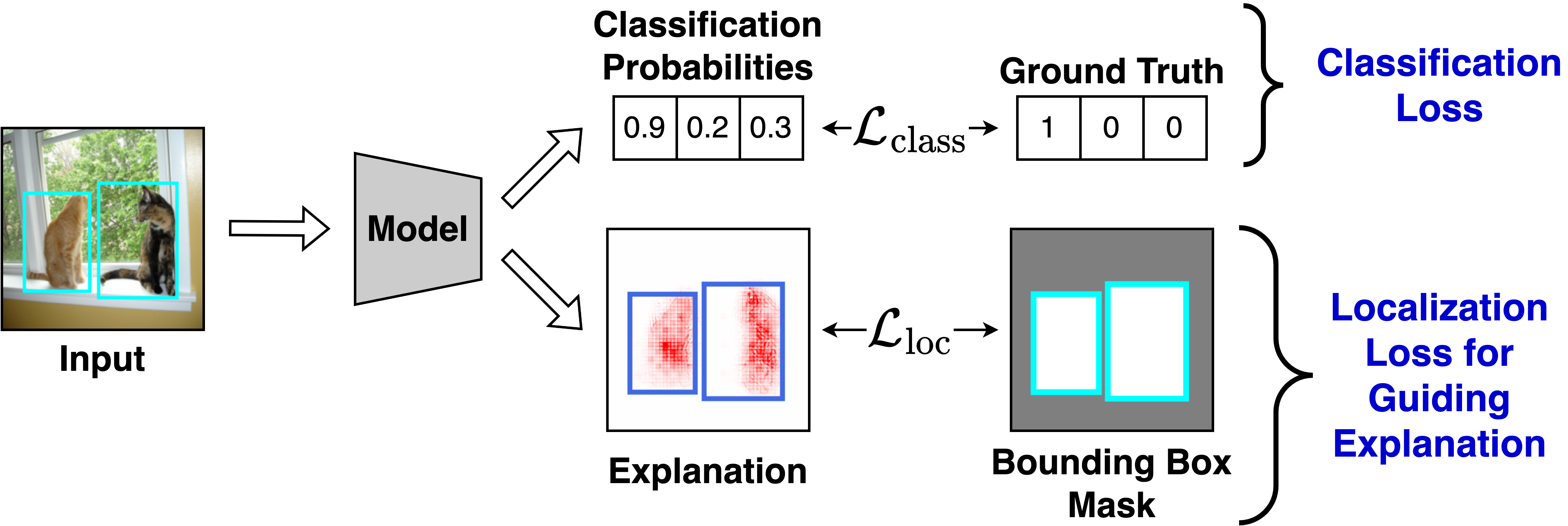
Fig. 3: Model guidance overview. We jointly optimize for classification ($\mathcal{L}_{\text{class}}$) and localization of attributions to human-annotated bounding boxes ($\mathcal{L}_{\text{loc}}$), to guide the model to focus on object features. Various localization loss functions can be used, see Sec. 3.4.

In this section, we provide an overview of the model guidance approach that jointly optimizes for classification and localization (Sec. 3.1). Specifically, we describe the attribution methods (Sec. 3.2), metrics (Sec. 3.3), and localization loss functions (Sec. 3.4) that we evaluate in Sec. 5. In Sec. 3.4.1 we then introduce our proposed Energy loss, and in Sec. 3.5 we discuss our strategy to train for localization in the presence of multiple ground truth classes.

Notation: We consider a multi-label classification problem with $K$ classes with $X\mkern 1.25mu{\in}\mkern 1.25mu\mathbb{R}^{C\times H\times W}$ the input image and $y\mkern 1.25mu{\in}\mkern 1.25mu\{0,1\}^{K}$ the one-hot encoding of the image labels. With $A_{k}\mkern 1.25mu{\in}\mkern 1.25mu\mathbb{R}^{H\times W}$ we denote an attribution map for a class $k$ for $X$ using a classifier $f$; $A_{k}^{+}$ denotes the positive component of the attributions, and $\hat{A}_{k}=\frac{A_{k}}{\max(A_{k})}$ normalized attributions. Finally, $M_{k}\mkern 1.25mu{\in}\mkern 1.25mu\{0,1\}^{H\times W}$ denotes the binary mask for class $k$, which is the given by the union of bounding boxes of all occurrences of class $k$ in $X$.

3.1 Model Guidance Procedure

Following prior work (e.g. [42, 49, 19, 18]), the model is trained jointly for classification and localization (cf. Fig. 3):

$$\textstyle\mathcal{L}=\mathcal{L}_{\text{class}}+\lambda_{\text{loc}}\mathcal{L}_{\text{loc}}\;.$$ (1)

I.e., the loss consists of a classification loss ($\mathcal{L}_{\text{class}}$), for which we use binary cross-entropy, and a localization loss ($\mathcal{L}_{\text{loc}}$), which we discuss in Sec. 3.4; here, the hyperparameter $\lambda_{\text{loc}}$ controls the weight given to each of the objectives.

3.2 Attribution Methods

In contrast to prior work that typically use GradCAM [46] attributions, we perform an evaluation over a selection of popularly used differentiable attribution methods which have been shown to localize well [39]: IxG [50], IntGrad [55], and GradCAM [46]. We further evaluate model-inherent explanations of the recently proposed B-cos models [6]. To ensure comparability across attribution methods [39], we evaluate all attribution methods at the input, various intermediate, and the final spatial layer.

GradCAM [46] is a popular method that weighs feature maps, typically at the final layer (i.e. last spatial layer), with pooled gradients with respect to the maps.

IxG [50] computes the element-wise product of the input and gradients with respect to the input, and serve as a faithful approximation of the contribution of a local neighbourhood in the input to the output.

IntGrad [55] takes an axiomatic approach and is formulated as the integral of gradients over a straight line path to the input from a baseline. Approximating this integral requires several gradient computations, making it computationally expensive for use in model guidance. To alleviate this, when optimizing with IntGrad, we use the recently proposed $\mathcal{X}$-DNN models [23] that efficiently compute IntGrad attributions by removing bias terms in the network.

B-cos [6] attributions are generated using the inherently-interpretable B-cos networks, which promote alignment between the input $\mathbf{x}$ and a dynamic weight matrix $\mathbf{W}(\mathbf{x})$ during optimization. In our experiments, we use the contribution maps given by the element-wise product of the dynamic weights with the input ($\mathbf{W}^{T}_{c}(\mathbf{x})\odot\mathbf{x}$), which faithfully represent the contribution of each pixel to class $c$. We also provide a differentiable implementation of B-cos explanations to use them for model guidance (supplement).

3.3 Evaluation Metrics

We evaluate the models’ performance on both our training objectives: classification and localization. For classification, we use the F1 score and mean average precision (mAP). We discuss the localization metrics below.

Intersection over Union (IoU) is a commonly used metric (cf. [18]) that thresholds the attributions to predict a binary mask and computes the ratio of the area of intersection with that of union of this mask with the bounding boxes. The optimal threshold is typically selected [15] via a heldout set.

Energy-based Pointing Game (EPG) [60] measures the concentration of attribution energy within the mask, i.e. the fraction of positive attributions inside the bounding boxes:

$$\text{EPG}_{k}=\frac{\sum_{h=1}^{H}\sum_{w=1}^{W}M_{k,hw}A^{+}_{k,hw}}{\sum_{h=1}^{H}\sum_{w=1}^{W}A^{+}_{k,hw}}\;.$$ (2)

In contrast to IoU, this is sensitive to the relative magnitude of attributions within an attribution map, and as a result more faithfully takes into account the importance given to each input region. Like IoU, the scores lie in $[0,1]$, with higher scores indicating better localization.

3.4 Localization Losses

We evaluate the most commonly used localization losses ($\mathcal{L}_{\text{loc}}$ in Eq. 1) from prior work. We describe these losses as applied on attribution maps of an image for a single class $k$, and propose our novel Energy loss (Sec. 3.4.1).

$L_{1}$ loss ([19, 18], Eq. 3) minimizes the $L_{1}$ distance between the annotation mask and the normalized positive attributions $A_{k}^{+}$, and guides the model to attribute uniformly to the existing highest attribution value within the mask, while suppressing attributions outside the mask.

$$\textstyle\mathcal{L}_{\text{loc},k}=\frac{1}{H\times W}\sum_{h=1}^{H}\sum_{w=1}^{W}\lVert M_{k,hw}-\hat{A}_{k,hw}^{+}\rVert_{1}$$ (3)

Per-pixel cross entropy (PPCE) loss ([49], Eq. 4) applies a binary cross entropy loss between the mask and the normalized positive annotations within the mask, and guides the model to maximize the attributions inside the mask:

$$\textstyle\mathcal{L}_{\text{loc},k}=-\frac{1}{\lVert M_{k}\rVert_{1}}\sum_{h=1}^{H}\sum_{w=1}^{W}M_{k,hw}\log(\hat{A}_{k,hw}^{+})\;.$$ (4)

However, since it does not apply any constraint on attributions outside the mask, there is no explicit pressure to the model to avoid spurious features.

RRR* loss ([42], Eq. 5). In [42], the authors introduced the RRR loss applied to the models’ gradients $\hat{A}_{k,hw}$ as

$$\textstyle\mathcal{L}_{\text{loc},k}=\sum_{h=1}^{H}\sum_{w=1}^{W}(1-M_{k,hw})\hat{A}_{k,hw}^{2}\;.$$ (5)

To extend it to our setting, we generalize this loss and take $\hat{A}_{k,hw}$ to be given by an arbitrary attribution method (e.g. IntGrad); we denote this generalized version by RRR*.

3.4.1 Energy Loss

As discussed in Sec. 3.4, existing localization losses do not constrain attributions across the entire input (RRR*, PPCE), or force the model to attribute uniformly within the mask even if it includes irrelevant background regions ($L_{1}$, PPCE). To mitigate this, inspired by the EPG metric ([60], Eq. 2), we propose a novel Energy localization loss to directly optimize for maximizing this metric (Eq. 6):

$$\textstyle\mathcal{L}_{\text{loc},k}=-\text{EPG}_{k}$$ (6)

In contrast to $L_{1}$ and PPCE, the Energy loss does not guide attributions to be uniform within the mask. Given that we use coarse bounding box annotations, this allows the model to focus on object features while ignoring the background regions within the bounding boxes. As such, this loss provides effective guidance while allowing the model to learn what to focus on within the bounding boxes, see Sec. 5.

3.5 Efficient Optimization

In contrast to prior work [42, 49, 19, 18], we perform model guidance on a multi-label classification setting, and consequently there are multiple ground truth classes whose attribution localization could be optimized. Computing and optimizing for several attributions within an image would add a significant overhead to the computational cost of training (multiple backward passes). Hence, for efficiency, we sample one ground truth class $k$ per image at random for every batch and only optimize for localization of that class, i.e., $\mathcal{L}_{\text{loc}}\mkern 1.25mu{=}\mkern 1.25mu\mathcal{L}_{\text{loc},k}$. We find that this still provides effective model guidance while keeping the training cost tractable.

4 Experimental Setup

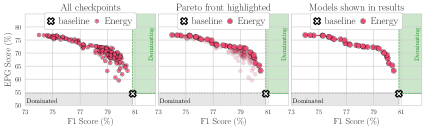
Fig. 4: Selecting models for evaluation. For each configuration, we evaluate every model at every checkpoint and measure its performance across various metrics (F1, EPG, IoU) on the validation set; i.e. every point in the left graph corresponds to one model (for B-cos models optimized via the Energy loss at the input layer). Instead of evaluating a single model on the test set, we evaluate all Pareto-dominant models, as indicated in the center and right plot.

In this section, we describe our experimental setup and how we select the best models across metrics. Full training details can be found in the supplement. We evaluate across the full sweep of combinations of choices for each category, and discuss our results in Sec. 5.

Datasets: We evaluate on PASCAL VOC 2007 [12] and MS COCO 2014 [28] for multi-label image classification. In Sec. 5.5, to understand the effectiveness of model guidance in mitigating spurious correlations, we also evaluate on the synthetically constructed Waterbirds-100 dataset [44, 35], where landbirds are perfectly correlated with land backgrounds on the training and validation sets, but are equally likely to occur on land or water in the test set (similar for waterbirds and water). With this dataset, we evaluate model guidance for suppressing undesired features.

Attribution Methods and Architectures: As described in Sec. 3.2, we evaluate with IxG [50], IntGrad [55], B-cos [6], and GradCAM [46] using models with a ResNet-50 [22] backbone. For IntGrad, we use an $\mathcal{X}$-DNN ResNet-50 [23] to reduce the computational cost, and a B-cos ResNet-50 for the B-cos attributions. We optimize the attributions at the input and final layer; for intermediate layer results, see supplement. Given the similarity of the results between GradCAM and IxG, and since B-cos attributions performed better than GradCAM for B-cos models, we show GradCAM results in the supplement. All models were pretrained on ImageNet [43], and model guidance was performed starting from a baseline model fine-tuned on the target dataset.

Localization Losses: As described in Sec. 3.4, we compare four localization losses in our evaluation: (i) Energy, (ii) $L_{1}$ [19, 18], (iii) PPCE [49], and (iv) RRR* (cf. Sec. 3.4, [42]).

Evaluation Metrics: As discussed in Sec. 3.3, we evaluate both for classification and localization performance of the models. For classification, we report the F1 scores, similar results with mAP scores can be found in the supplement. For localization, we evaluate using the EPG and IoU scores.

Selecting the best models: As we evaluate for two distinct objectives (classification and localization), it is non-trivial to decide which models to select during training. E.g., a model that provides the best classification performance might provide significantly worse localization performance than a model that provides slightly lower classification performance but much better localization. Finding the right balance and deciding which of those models in fact constitutes the ‘better’ model depends on the preference of the end user. Hence, instead of selecting models based on a single metric, we select the set of Pareto-dominant models [33, 34, 5] across three metrics—F1, EPG, and IoU—for each training configuration, as defined by a combination of attribution method, layer, and loss. Specifically, as shown in Fig. 4, we train for each configuration using three different choices of $\lambda_{\text{loc}}$, and select the set of Pareto-dominant models among all checkpoints (epochs and $\lambda_{\text{loc}}$). This provides a more holistic view of the general trends on the effectiveness of model guidance for each configuration.

5 Experimental Results

(a) PASCAL VOC results for EPG vs. F1.

(b) MS COCO results for EPG vs. F1.

Fig. 5: EPG vs. F1, for different datasets ((a): VOC; (b): COCO), losses (markers) and models (columns), optimized at different layers (rows); additionally, we show the performance of the baseline model before fine-tuning and demarcate regions that strictly dominate (are strictly dominated by) the baseline performance in green (grey). For each configuration, we show the Pareto fronts (cf. Fig. 4) across regularization strengths $\lambda_{\text{loc}}$ and epochs (cf. Sec. 5 and Fig. 4). We find the Energy loss to give the best trade-off between EPG and F1.

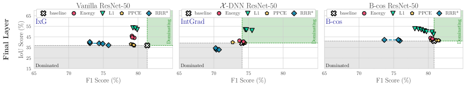
Fig. 6: IoU vs. F1, for different losses (markers) and models (columns) for VOC; results for COCO are in the supplement. Additionally, we show the performance of the baseline model before fine-tuning and demarcate regions that strictly dominate (are strictly dominated by) the baseline model in green (grey). For each configuration, we show the Pareto fronts (Fig. 4) across regularization strengths $\lambda_{\text{loc}}$ and all epochs; for details, see Secs. 4, LABEL: and 5. Across all configurations, we find the $L_{1}$ loss to provide the largest gains in IoU at the lowest cost.

In this section, we discuss our experimental findings. In particular, in Sec. 5.1, we first discuss the impact of the loss functions on the EPG and IoU scores of the models; in Sec. 5.2, we then analyze the impact of the models and attribution methods; further in Sec. 5.3, we show that guiding the models via their explanations can even lead to improved classification accuracy. In Sec. 5.4, we present two ablation studies in which we evaluate and discuss the cost of model guidance approaches: in particular, we study model guidance with limited additional labels and with increasingly coarse bounding boxes. Finally, in Sec. 5.5, we show the utility of model guidance in improving accuracy in the presence of distribution shifts. For easier reference, we further label our individual findings as R1–R8.

Note. To draw conclusive insights and highlight general and reliable trends in the experiments, we compare the Pareto curves (see Fig. 4) of individual configurations. If the Pareto curve of a specific loss (e.g. Energy in Fig. 5) consistently Pareto-dominates the Pareto curves of all other losses, we can confidently conclude that for the combination of evaluated metrics (e.g. EPG vs. IoU), this loss is the best choice.

5.1 Comparing loss functions for model guidance

In the following, we highlight the main insights gained from the quantitative evaluations. For a qualitative comparison between the losses, please see Fig. 7; note that we show examples for a B-cos models as the differences become clearest—full results are shown in the supplement.

R1 The energy loss yields the best EPG scores. In Fig. 5, we plot the Pareto curves for EPG vs. F1 scores for a wide range of configurations (see Sec. 4) on VOC (a) and COCO (b); specifically, we group the results by model type (Vanilla, $\mathcal{X}$-DNN, B-cos), the layer depths at which the attribution was regularized (Input / Final), and the loss used during optimization (Energy, $L_{1}$, PPCE, RRR*). From these results it becomes apparent that the optimization with the energy loss yields the best trade-off between accuracy (F1) and the EPG score: e.g., when looking at the upper right plot in Fig. 5(a) we can see that the Energy loss (red dots) improves over the baseline B-cos model (white cross) by improving the localization in terms of EPG score with only a minor cost in classification performance (i.e. F1 score). Further trading off F1 scores yields even higher EPG scores. Importantly, the Energy loss Pareto-dominates all the other losses (RRR*: blue diamonds; $L_{1}$: green triangles; PPCE: yellow pentagons). This is is also true for the other networks (Vanilla ResNet-50, Fig. 5(a) (top left), and $\mathcal{X}$-DNN, Fig. 5(a) (top center)) and at the final layer (bottom row). When comparing Fig. 5(a) and Fig. 5(b), we find these results to be highly consistent between datasets.

R2 The $L_{1}$ loss yields the best IoU performance. Similarly, in Fig. 6, we plot the Pareto curves of IoU vs. F1 scores for various configurations at the final layer; for the IoU results at the input layer and on the COCO dataset, please see the supplement. For IoU, the $L_{1}$ loss provides the best trade-off and, with few exceptions, $L_{1}$-guided models Pareto-dominate all other models in all configurations.

R3 The Energy loss focuses best on class-specific features. By not forcing the models to highlight all features within the bounding boxes (see Sec. 3.4.1), we qualitatively find it to preserve more detail (cf. Figs. 7, LABEL: and 9) and to suppress background features also within the bounding boxes. This qualitative observation is confirmed when measuring the Energy (Eq. 2) just withing the bounding boxes: for this, we take advantage of the segmentation mask annotations available for a subset of the VOC test set. Specifically, we measure the energy contained in the segmentation masks versus the entire bounding box, which indicates how much of the attributions actually highlight on-object features. We find that the energy loss outperforms $L_{1}$ across all models and configurations; for details, please see the supplement.

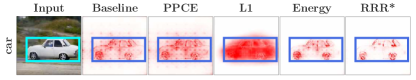
Fig. 7: Loss comparison for input attributions (atts.) of a B-cos model. We show atts. before (baseline, col. 2) and after guidance (cols. 3-6) for a specific image (col. 1) and its bounding box annotation. We find that Energy and RRR* yield sparse atts, whereas $L_{1}$ yields smoother atts, as it is optimized to fill the entire bounding box. For PPCE we observe only a minor effect on the atts.

In short, we find that the Energy loss works best for improving the EPG metric, whereas the $L_{1}$ loss yields the highest gains in terms of IoU; depending on the use case, either of these losses could thus be recommendable. However, we find that the Energy loss is more robust to annotation errors (R8, Sec. 5.4), and, as discussed in R3, the Energy loss more reliably focuses on object-specific features.

5.2 Comparing models and attribution methods

In the following, we highlight our findings with respect to differences between attribution methods and models.

R4 At the input layer, B-cos explanations perform best. We find that the B-cos models not only achieve the highest EPG/IoU performance before fine-tuning the models (‘baselines’), but also obtain the highest gains in EPG and IoU and thus the highest overall performance (for EPG see Fig. 5, right; for IoU, see supplement): e.g., an Energy-based B-cos model achieves an EPG score of 71.7 @ 79.4%F1, thus significantly outperforming the best EPG scores of both other model types at a much lower cost in F1 (Vanilla: 55.8 @ 69.0%, $\mathcal{X}$-DNN: 62.3 @ 68.9%). This is also observed qualitatively, as we show in the supplement.

R5 Regularizing at the final layer yields consistent gains. As can be seen in Fig. 5 (bottom) and 6, all models can be ‘guided’ well when applying regularization at the final layer and show improvements in IoU as well as the EPG score.

In short, we find model guidance to work well across all tested models when optimizing at the final layer (R5), highlighting its wide applicability. However, to obtain highly detailed and well-localized attributions at the input layer, the model-inherent explanations of the B-cos models seem to lend themselves much better to such guidance (R4).

5.3 Improving accuracy with model guidance

R6 Model guidance can improve accuracy. For both the Vanilla models (final layer) and the $\mathcal{X}$-DNNs (input+final), we found models that improve the localization metrics and the F1 score. These improvements are particularly pronounced for the $\mathcal{X}$-DNN: e.g., we find models that improve the EPG and F1 scores by $\Delta\mkern 1.25mu{=}\mkern 1.25mu7.2$ p.p.  and $\Delta\mkern 1.25mu{=}\mkern 1.25mu1.4$ p.p. respectively (Fig. 5, center top), or the IoU and F1 scores by $\Delta\mkern 1.25mu{=}\mkern 1.25mu1.4$ p.p. and $\Delta\mkern 1.25mu{=}\mkern 1.25mu11.9$ p.p. (Fig. 6, center).

However, overall we observe a trade-off between localization and accuracy (Figs. 5 and 6). Given the similarity of the training and test distributions, focusing on the object need not improve classification performance, as spurious features are also present at test time. Further, the guided model is discouraged from relying on contextual features, making the classification more challenging. In Sec. 5.5, we show that guidance can significantly improve performance when there is a distribution shift between training and test.

5.4 Efficiency and robustness considerations

Guiding models via bounding boxes of course requires additional annotation effort, increasing the cost of data collection. In this section, we therefore assess the robustness of guiding the model with a limited number of annotations (R7) and with increasingly coarse annotations (R8).

R7 Model guidance requires only few add. annotations. In Fig. 10, we show that the EPG score can be significantly improved with a very limited number of annotations; for IoU results, see supplement. Specifically, we find that when using only 1% of the training data (25 annotated images) for VOC, improvements of up to $\Delta\mkern 1.25mu{=}\mkern 1.25mu23.0$ p.p. ($\Delta\mkern 1.25mu{=}\mkern 1.25mu1.4$) in EPG (IoU) can be obtained, at a minor drop in F1 ($\Delta\mkern 1.25mu{=}\mkern 1.25mu0.3$ p.p. and $\Delta\mkern 1.25mu{=}\mkern 1.25mu2.5$ p.p. respectively). When annotating up to 10% of the images, very similar results can be achieved as with full annotation (see e.g. cols. 2+3 in Fig. 10).

R8 The energy loss is highly robust to annotation errors. As discussed in Sec. 3.4.1, the energy loss only ‘tells’ the model which features not to use and does not impose a uniform prior on the attributions within the bounding boxes. As a result, we find it to be much more stable to annotation errors: e.g., in Fig. 8, we visualize how the EPG (top) and IoU (bottom) scores of the best performing models under the Energy (left) and $L_{1}$ loss (right) evolve when using coarser bounding boxes; for this, we simply dilate the bounding box size by $p\mkern 1.25mu{\in}\mkern 1.25mu\{10,25,50\}$% during training, see Fig. 9. While the models optimized via the $L_{1}$ loss achieve increasingly worse results (right), the Energy-optimized models are essentially unaffected by the coarseness of the annotations.

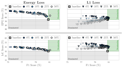
Fig. 8: Quantitative results for dilated bounding boxes for a B-cos model at the input layer. We show EPG and IoU (top and bottom) results for models trained with various amounts of annotation errors (increasingly large bounding boxes, see Fig. 9). The Energy loss yields highly consistent results despite training with heavily dilated bounding boxes (left), whereas the results of the $L_{1}$ loss (right) worsen markedly.

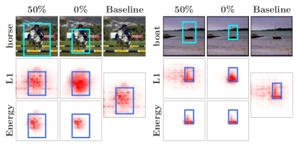
Fig. 9: Qualitative results for dilated bounding boxes for a B-cos model at input. Examples for attributions (rows 2+3) of models trained with dilated bounding boxes (row 1). In contrast to $L_{1}$, models trained with Energy show significant gains in object focus even with significant noise (e.g. ‘Baseline’ vs. ‘50%’).

In short, we find that the models can be guided effectively at a low cost in terms of annotation effort, as only few annotations (e.g. 25 for VOC) are required (cf. R7), and, especially for the Energy loss, these annotations can be very coarse and do not have to be ‘pixel-perfect’ (cf. R8).

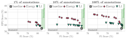
Fig. 10: EPG results with limited annotations for a B-cos model at the input layer, optimized with the Energy and the $L_{1}$ loss. Using bounding box annotations for as little as 1% (left) of the images yields significant improvements in EPG, and with 10% (center) similar gains as in the fully annotated setting (right) are obtained.

5.5 Effectiveness against spurious correlations

To evaluate the potential for mitigating spurious correlations, we evaluate model guidance with the Energy and $L_{1}$ losses on the synthetically constructed Waterbirds-100 dataset [44, 35]. We perform model guidance under two settings: (1) the conventional setting to classify between landbirds and waterbirds, using the region within the bounding box as the mask; and (2) the reversed setting [35] to classify the background, i.e., land vs. water, using the region outside the bounding box as the mask. To simulate a limited annotation budget, we only use bounding boxes for a random 1% of the training set, and report results averaged over four runs. We show the results for the worst-group accuracy (i.e., images containing a waterbird on land) and the overall accuracy using B-cos models in Tab. 1; full results for all attributions and models can be found in the supplement.

Both losses consistently and significantly improve the accuracy in the conventional and the reversed settings by guiding the model to select the ‘right’ features, i.e. birds (conventional) or background (reversed). This guidance can also be observed qualitatively (cf. Fig. 11).

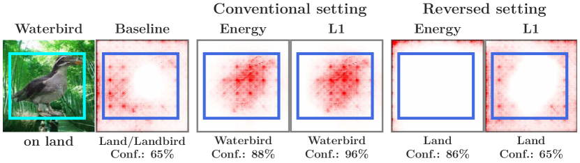
Fig. 11: Qualitative Waterbirds-100 results. A non-guided model might focus on the background to classify birds (baseline) and thus misclassify waterbirds on land (col. 2). Guided models can correct such errors and focus on the desired feature: in cols. 3+4 (5+6) the model is guided to classify by using the bird (background) features and arrives at the desired prediction. Model prediction (+confidence) shown below the images.

	Conventional		Reversed
Model	Worst	Overall	Worst	Overall
Baseline	43.4 ($\pm$2.4)	68.7 ($\pm$0.2)	56.6 ($\pm$2.4)	80.1 ($\pm$0.2)
Energy	56.1 ($\pm$4.0)	71.2 ($\pm$0.1)	62.8 ($\pm$2.1)	83.6 ($\pm$1.1)
$L_{1}$	51.1 ($\pm$1.9)	69.5 ($\pm$0.2)	58.8 ($\pm$5.0)	82.2 ($\pm$0.9)

Table 1: Evaluation on the Waterbirds-100 dataset. We find that model guidance is effective in improving both worst-group and overall accuracy in the conventional (Landbird vs. Waterbird) and reversed (Land vs. Water) settings; full results in the supplement.

6 Discussion And Conclusion

In this work, we comprehensively evaluated various models, attribution methods, and loss functions for their utility in guiding models to be “right for the right reasons”.

In summary, we find that guiding models via bounding boxes can significantly improve EPG and IoU performance of the optimized attribution method, with the Energy loss working best to improve the EPG score (R1) and the $L_{1}$ loss yielding the highest gains in IoU scores (R2). While the B-cos models achieve the best results in IoU and EPG score at the input layer (R4), all tested model types (Vanilla, $\mathcal{X}$-DNN, B-cos) lend themselves well to being optimized at the final layer (R5). Further, we find that regularizing the explanations of the models and thereby ‘telling them where to look’ can even increase the object recognition performance (mAP/accuracy) of some models (R6), especially when strong spurious correlations are present (Sec. 5.5). Interestingly, those gains (EPG, IoU), can be achieved with relatively little additional annotation (R7). Lastly, we find that by not assuming a uniform prior over the attributions within the annotated bounding boxes, training with the energy loss is more robust to annotation errors (R8) and results in models that produce attribution maps that are more focused on class-specific features (R3).

Table of Contents

In this supplement to our work on using explanations to guide models, we provide:

1. Additional qualitative results (VOC and COCO) A
   In this section, we present additional qualitative results. In particular, we provide:

   (A.1)    Detailed comparisons between models, layers, and losses. (VOC + COCO).
   (A.2)    Additional visualizations for training with dilated bounding boxes (VOC + COCO).
   

2. Additional quantitative results (VOC and COCO) B
   In this section, we present additional quantitative results. In particular, we show:

   (B.1)    The remaining localization vs. accuracy comparisons (VOC + COCO).
   (B.2)    The results of guiding models via GradCAM. (VOC + COCO).
   (B.3)    Results for optimizing at intermediate layers (VOC).
   (B.4)    Results for measuring on-object EPG scores (VOC).
   (B.5)    Additional analyses regarding training with few annotated images (VOC).
   (B.6)    Additional analyses regarding the usage of coarse bounding boxes (VOC).
   

3. Additional results on the Waterbirds dataset C
   In this section, we provide additional results for the Waterbirds-100 dataset. In particular, we provide full results regarding classification performance with and without model guidance as well as additional qualitative visualizations of the attribution maps.
   

4. Implementation details D
   In this section, we provide relevant implementation details; note that all code will be made available upon publication. In particular, we provide:

   (D.1)    Training details across datasets (VOC + COCO + Waterbirds).
   (D.2)    Implementation details for twice-differentiable B-cos models.
   

5. Full results across all experiments. X
   Given the large amount of experimental results, in each of the preceding sections we show only a sub-selection of those results for improved readability. In section X, we provide the full results across datasets, models, layers, experiments, and metrics, to peruse at the reader’s convenience.  
   

Appendix A Additional Qualitative Results (VOC and COCO)

A.1 Qualitative Examples Across Losses, Attribution Methods, and Layers

PASCAL VOC 2007.

Input

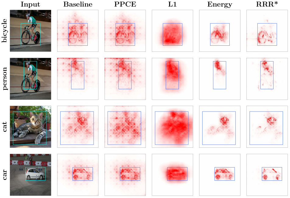
Final

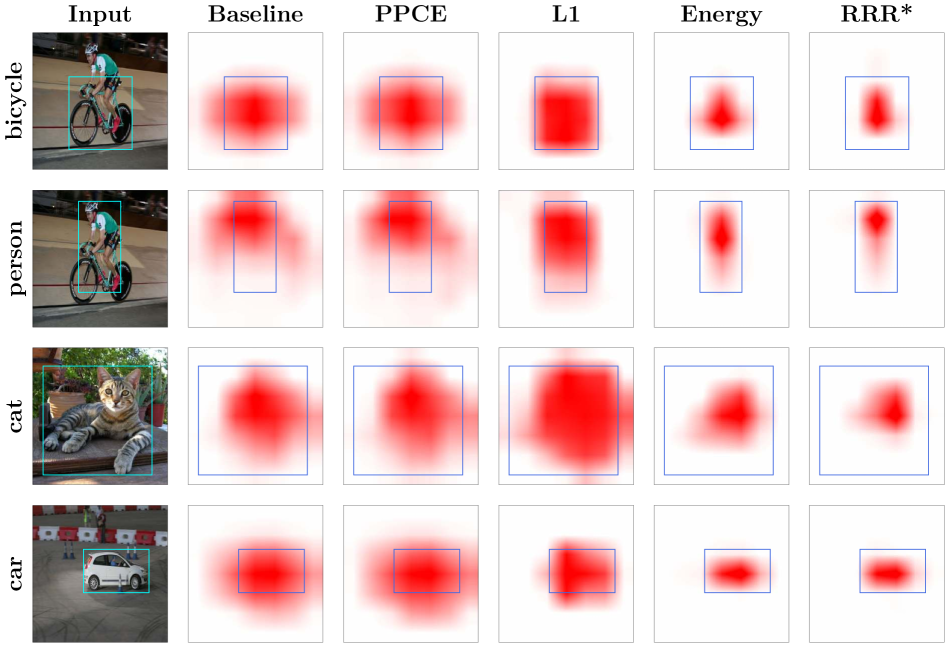
(a) B-cos ResNet-50.

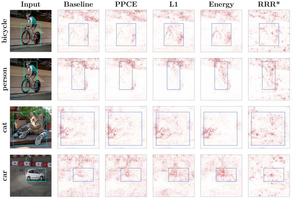
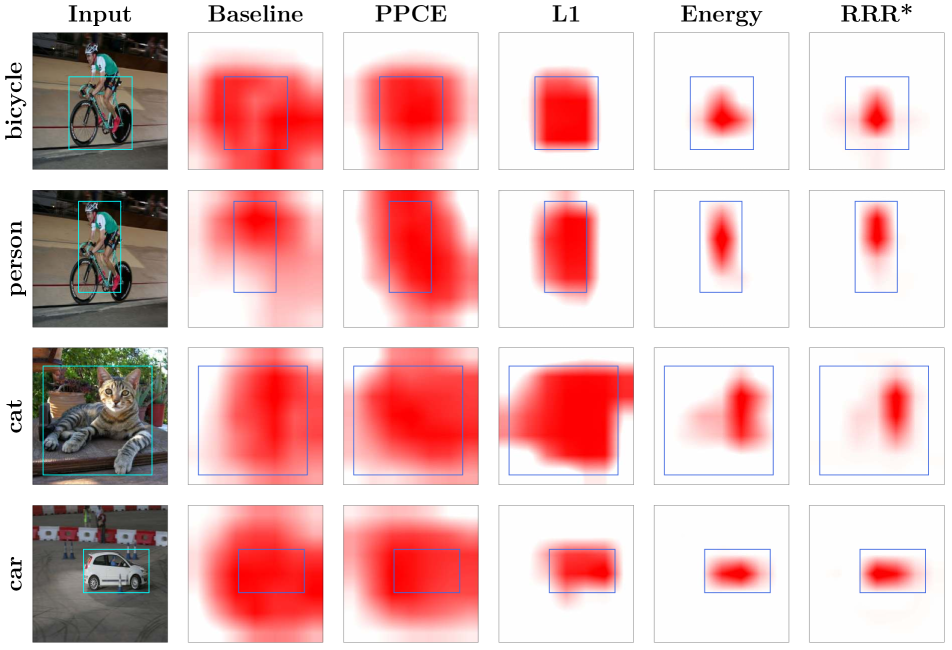
(b) Vanilla ResNet-50.

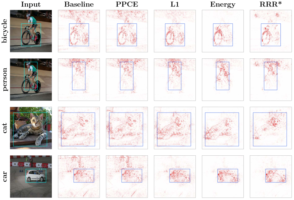
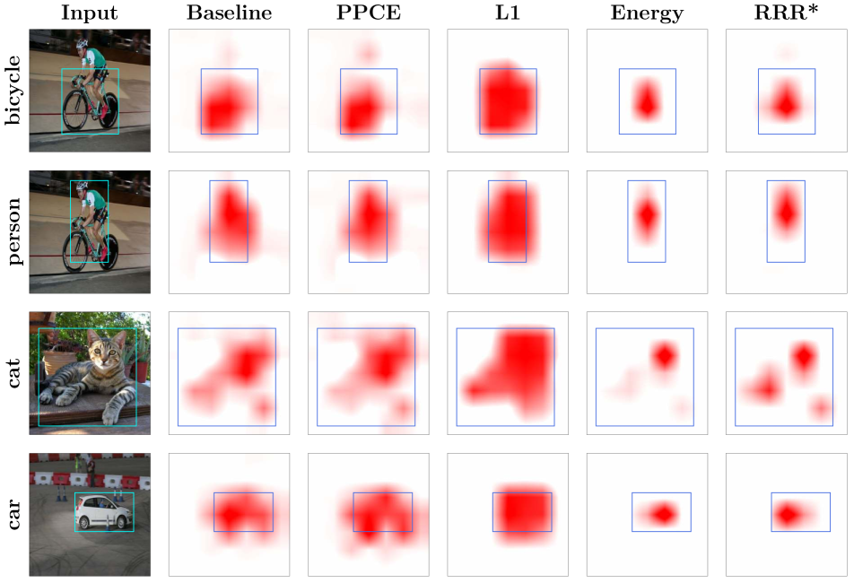
(c) $\mathcal{X}$-DNN ResNet-50.

Fig. A2: Qualitative examples from the VOC dataset. In particular, this figure allows to compare between models (major rows, i.e. (a), (b), and (c)) losses (major columns) and layers (left+right) for multiple images (minor rows).

MS COCO 2014.

Input

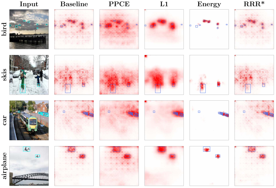
Final

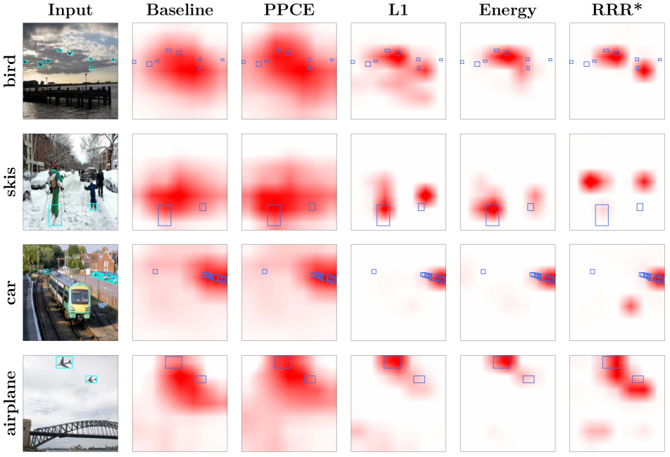
(a) B-cos ResNet-50.

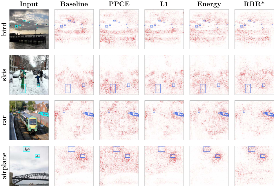
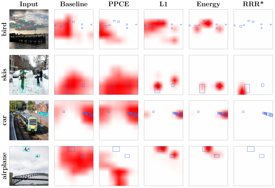
(b) Vanilla ResNet-50.

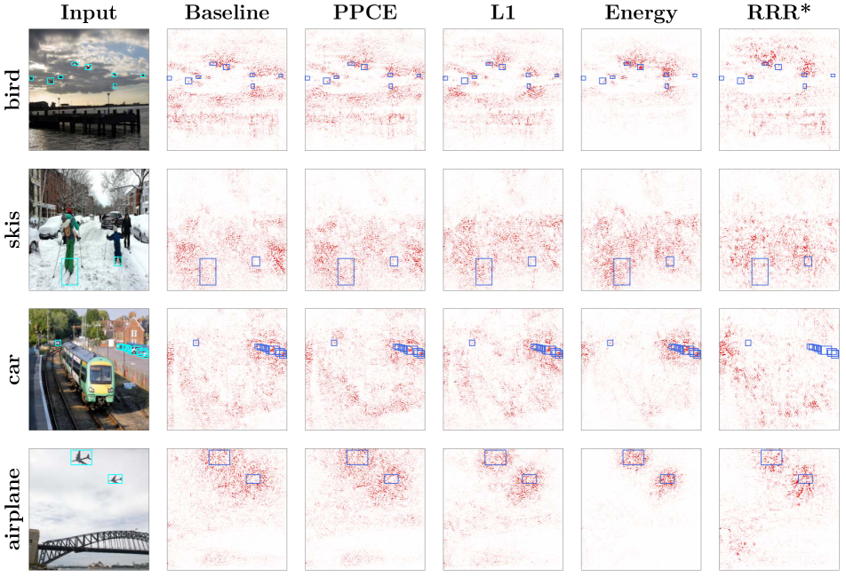
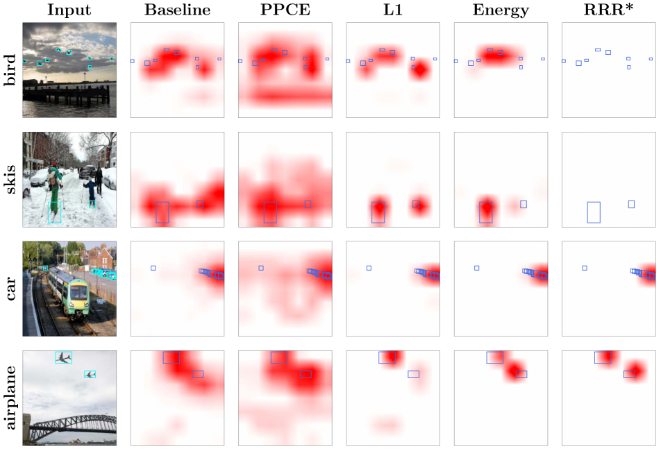
(c) $\mathcal{X}$-DNN ResNet-50.

Fig. A4: Qualitative examples from the COCO dataset. In particular, this figure allows to compare between models (major rows, i.e. (a), (b), and (c)) losses (major columns) and layers (left+right) for multiple images (minor rows).

Additional qualitative examples.

PASCAL VOC 2007

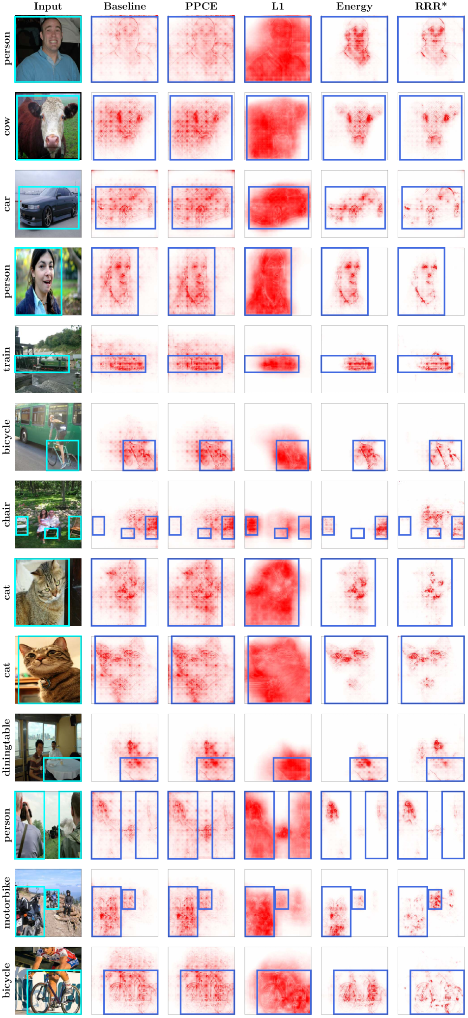
MS COCO 2014

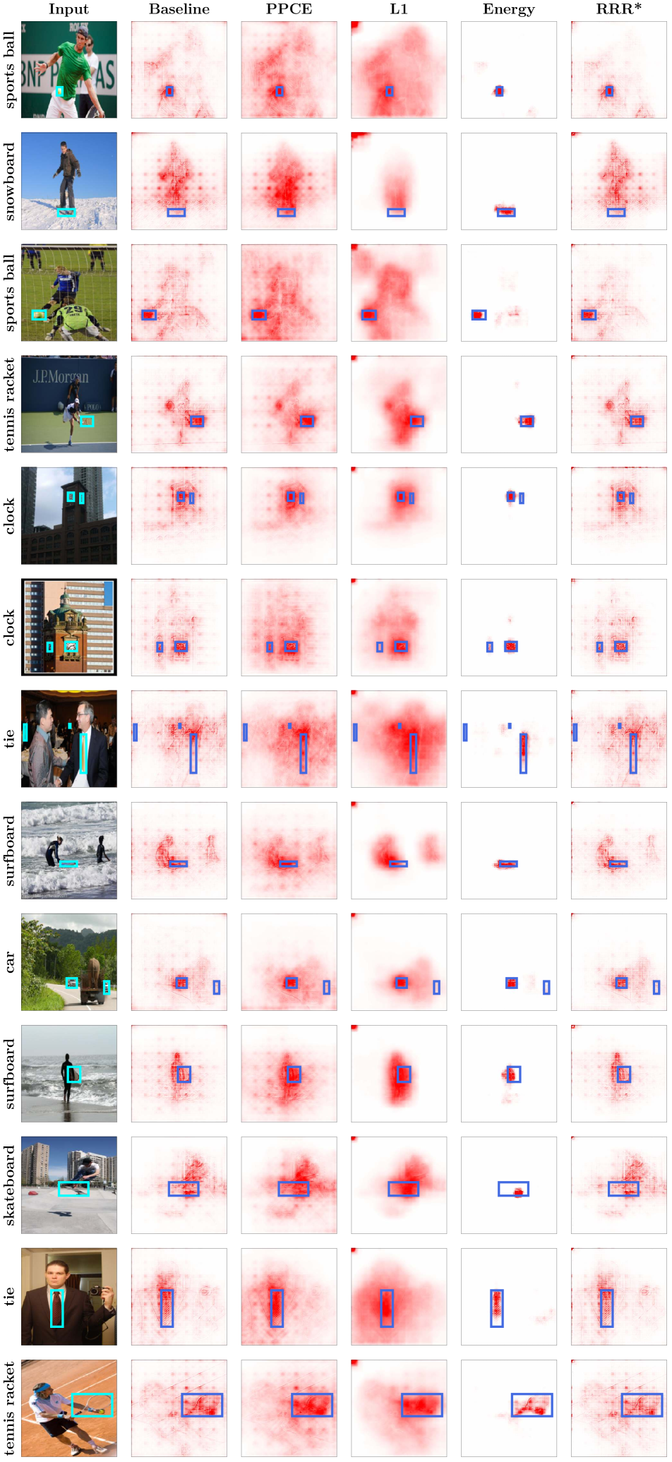
Fig. A6: Qualitative examples from the VOC (left) and COCO (right) datasets. In particular, here we just show additional examples for the B-cos models with input attributions, as this configuration exhibits the most detail. We show results for such models trained with different losses (columns) for multiple images (rows).

In Figs. A2 and A4, we visualize attributions across losses, attribution methods, and layers for the same set of examples from the VOC and COCO datasets respectively. As discussed in the main paper, we make the following observations.

First, when guiding models at the final layer, we observe a marked improvement in the granularity of the attribution maps for all losses (R5), except for PPCE, for which we do not observe notable differences. The improvements are particularly noticeable on the COCO dataset (Fig. A4, “Final” column), in which the objects tend to be smaller. E.g., when looking at the airplane image (last row per model), we observe much fewer attributions in the background after applying model guidance.

Second, as the $L_{1}$ loss optimizes for uniform coverage within the bounding boxes, it provides coarser attributions that tend to fill the entire bounding box (cf. R3). This can be observed particularly well for the large objects from the VOC dataset: e.g., whereas models trained with the Energy and the RRR loss highlight just a relatively small area within the bounding box of the cat (Fig. A2, ”Final” column, third row), the $L_{1}$ loss yields much more distributed attributions for all models.

Third, at the input layer, the B-cos models show the most notable qualitative improvements (cf. R4). In particular, although the $\mathcal{X}$-DNN models show some reduction in noisy background attributions (e.g. last rows in Fig. 2(c) and Fig. 4(c)), the attributions remain rather noisy for many of the images; for the Vanilla models, the improvements are even less pronounced (Fig. 2(b), Fig. 4(b)). The B-cos models, on the other hand, seem to lend themselves better to such guidance being applied to the attributions at the input layer (Fig. 2(a), Fig. 4(a)) and the resulting attributions show much more detail (Energy + RRR) or an increased focus on the entire bounding box ($L_{1}$). Especially with the Energy, the B-cos models are able to clearly focus on even small objects, see Fig. 4(a).

For additional results from both the VOC as well as the COCO dataset, please see Fig. A6.

A.2 Additional visualizations for training with coarse bounding boxes

In this section, we show more detailed and additional examples of models trained with coarser bounding boxes, i.e. with bounding boxes that are purposefully dilated during training by various amounts (10%, 25%, or 50%), see Fig. A7. In accordance with our findings in the main paper (cf. R8), we observe that the Energy loss is highly robust to such ‘annotation errors’: the attribution maps improve noticeably in all cases (compare the Energy row with the respective baseline result). In contrast, the $L_{1}$ loss seems more dependent on high-quality annotations, which we also observe quantitatively, see Fig. B9.

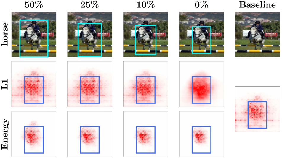
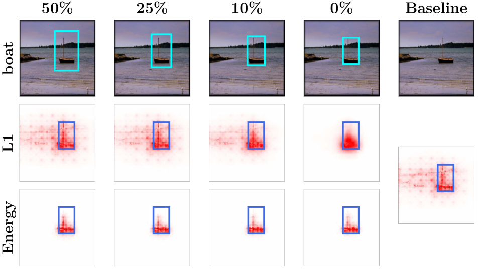
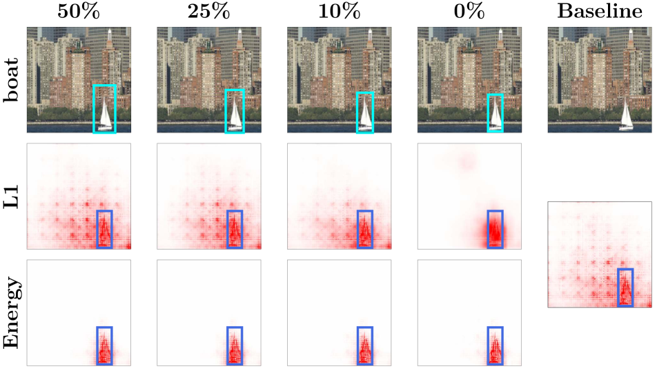
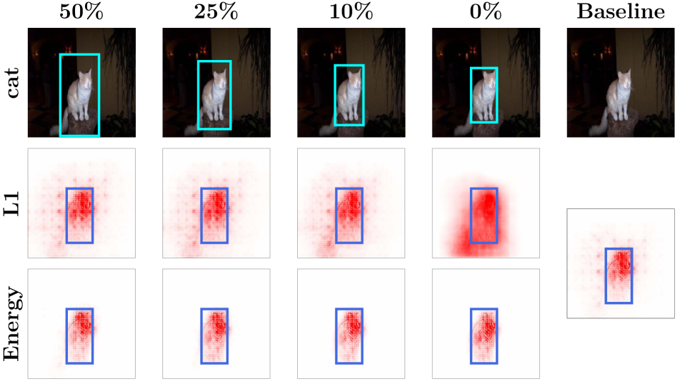
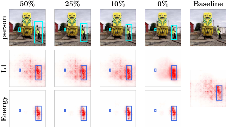
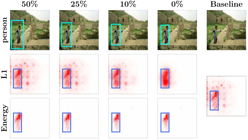
Fig. A7: Qualitative examples of the impact of using coarse bounding boxes for guidance. We show examples of B-cos attributions from the input layer on the baseline model and on models guided with the Energy and $L_{1}$ localization losses with varying degrees of dilation $\{10\%,25\%,50\%\}$ in bounding boxes during training. For each example (block in the figure), we show the image and bounding boxes with varying degrees of dilation (top row), attributions with the $L_{1}$ localization loss (middle row), and attributions with the Energy localization loss (bottom row). We find that in contrast to using the $L_{1}$ localization loss, guidance with Energy localization loss maintains localization of attributions to on-object features even with dilated bounding boxes. Note that bounding boxes are dilated only during training, not during evaluation. Bounding boxes in light blue show the extent of dilation that would have been used had the image been from the training set, while those in dark blue show undilated bounding boxes that are used during evaluation.

Appendix B Additional Quantitative Results (VOC and COCO)

In this section, we provide additional quantitative results from our experiments on the VOC and COCO datasets. Specifically, in Sec. B.1, we show additional results comparing classification and localization performance. In Sec. B.2 we present results for guiding models via GradCAM attributions. In Sec. B.3, we show that training at intermediate layers can be a cost-effective way approach to performing model guidance. In Sec. B.4, we evaluate how well the attributions localize to on-object features (as opposed to background features) within the bounding boxes, and find that the Energy outperforms other localization losses in this regard. In Sec. B.5, we provide additional analyses regarding training with a limited number of annotated images. Finally, in Sec. B.6, we provide additional analyses regarding the usage of coarse, dilated bounding boxes during training.

B.1 Comparing Classification and Localization Performance

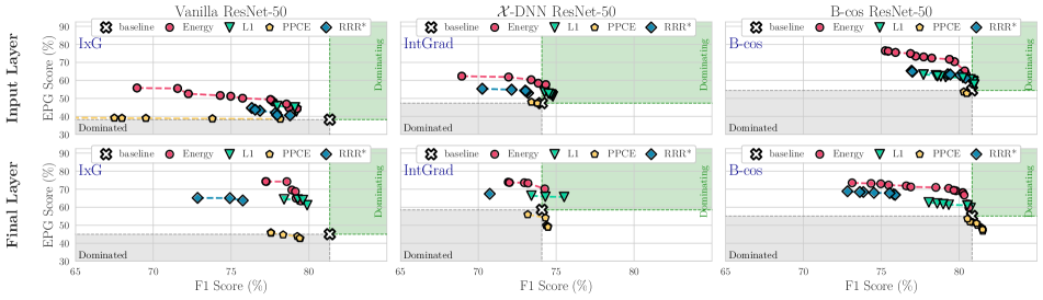
(a) EPG vs. F1.

(b) IoU vs. F1.

Fig. X1: EPG (a) and IoU (b) vs. F1 on VOC, for different losses (markers) and models (columns), optimized at different layers (rows); additionally, we show the performance of the baseline model before fine-tuning and demarcate regions that strictly dominate (are strictly dominated by) the baseline performance in green (grey). For each configuration, we show the Pareto fronts (cf. Fig. 4) across regularization strengths $\lambda_{\text{loc}}$ and epochs (cf. Sec. 5 and Fig. 4). We find the Energy loss to give the best trade-off between EPG and F1, whereas the $L_{1}$ loss (especially at the final layer) provides the best trade-off between IoU and F1. We further find these results to be consistent across datasets, see Fig. X2.

In this section, we discuss additional quantitative findings with respect to localization and classification performance metrics (IoU, mAP) for a selected subset of the experiments; for a full comparison of all layers and metrics, please see Figs. X1, LABEL:, X2, LABEL:, X3, LABEL: and X4.

Additional IoU results. In Figs. B1 and B2, we show the remaining results comparing IoU vs. F1 scores that were not shown in the main paper for VOC and COCO respectively. Similar to the results in the main paper for the EPG metric (Fig. 5), we find that the results between datasets are highly consistent for the IoU metric.

In particular, as discussed in Sec. 5.1, we find that the $L_{1}$ loss yields the largest improvements in IoU when optimized at the final layer, see bottom rows of Figs. B1, LABEL: and B2. At the input layer, we find that Vanilla and $\mathcal{X}$-DNN ResNet-50 models are not improving their IoU scores noticeably, whereas the B-cos models show significant improvements. We attribute this to the noisy patterns in the attribution maps of Vanilla and $\mathcal{X}$-DNN models, which might be difficult to optimize.

IoU results on VOC.

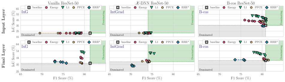
Fig. B1: IoU results on PASCAL VOC 2007. We show IoU vs. F1 for all localization loss functions, attribution methods, and layers. In contrast to the consistent improvements observed at the final layer with the $L_{1}$ loss, the IoU metric only noticeably improves for the B-cos models after model guidance. We attribute this to the high amount of noise present in the attribution maps of Vanilla and $\mathcal{X}$-DNN models, see e.g. Figs. A2, LABEL: and A4. For results on the COCO dataset, please see Fig. B2.

IoU results on COCO.

Fig. B2: IoU results on MS COCO 2014. We show IoU vs. F1 for all localization loss functions, attribution methods, and layers. In contrast to the consistent improvements observed at the final layer with the $L_{1}$ loss, the IoU metric only noticeably improves for the B-cos models after model guidance. We attribute this to the high amount of noise present in the attribution maps of Vanilla and $\mathcal{X}$-DNN models, see e.g. Figs. A2, LABEL: and A4. For results on the VOC dataset, please see Fig. B1.

Using mAP to evaluate classification performance. In all results so far, we plotted the localization metrics (EPG, IoU) versus the F1 score as a measure of classification performance. In order to highlight that the observed trends are independent of this particular choice of metric, in Fig. B3, we show both EPG as well as IoU results plotted against the mAP score.

In general, we find the results obtained for the mAP metric to be highly consistent with the previously shown results for the F1 metric. E.g., across all configurations, we find the Energy to yield the highest gains in EPG score, whereas the $L_{1}$ loss provides the best trade-offs with respect to the IoU metric. In order to easily compare between all results for all datasets and metrics, please see Figs. X1, LABEL:, X2, LABEL:, X3, LABEL: and X4.

Mean Average Precision (mAP) results on VOC.

(a) EPG vs. mAP.

(b) IoU vs. mAP.

Fig. B3: Quantitative comparison of EPG and IoU vs. mAP scores for VOC. To ensure that the trends observed and described in the main paper generalize beyond the F1 metric, in this figure we show the EPG and IoU scores plotted against the mAP metric. In general, we find the results obtained for the mAP metric to be highly consistent with the previously shown results for the F1 metric, see e.g. Figs. 5, LABEL: and 6. E.g., across all configurations, we find the Energy to yield the highest gains in EPG score, whereas the $L_{1}$ loss provides the best trade-offs with respect to the IoU metric. To compare between all results for all datasets and metrics, please see Figs. X1, LABEL:, X2, LABEL:, B3, LABEL: and X4.

B.2 Model Guidance via GradCAM

Comparison to GradCAM on VOC.

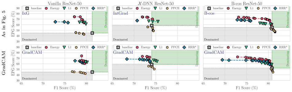
Fig. B4: Quantitative results using GradCAM. We show EPG scores vs. F1 scores for all localization losses and models using GradCAM at the final layer (bottom row) and compare it to the results shown in the main paper (top row). As expected, GradCAM performs very similarly to IxG (Vanilla) and IntGrad ($\mathcal{X}$-DNN) used at the final layer—in particular, note that for ResNet-50 architectures, IxG and IntGrad are very similar to GradCAM for Vanilla and $\mathcal{X}$-DNN models respectively (see Sec. B.2). Similarly, we find GradCAM to also perform comparably to the B-cos explanations when used at the final layer; for IoU results and results on COCO, see Figs. X5, LABEL: and X6.

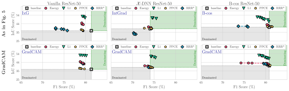
(b) IoU vs. F1.

Fig. X5: Quantitative results using GradCAM on VOC. We show EPG (a) and IoU (b) scores vs. F1 scores for all localization losses and models using GradCAM at the final layer (bottom rows in (a)+(b) and compare it to the results shown in the main paper (top rows). As expected, GradCAM performs very similarly to IxG (Vanilla) and IntGrad ($\mathcal{X}$-DNN) used at the final layer—in particular, note that for ResNet-50 architectures, IxG and IntGrad are very similar to GradCAM for Vanilla and $\mathcal{X}$-DNN models respectively (see Sec. B.2). Similarly, we find GradCAM to also perform comparably to the B-cos explanations when used at the final layer; for results on COCO, see Fig. X6.

In Fig. B4, we show the EPG vs. F1 results of training models with GradCAM applied at the final layer on the VOC dataset; for IoU results and results on COCO, please see Figs. X5 and X6. When comparing between rows (top: main paper results; bottom: GradCAM), it becomes clear that GradCAM performs very similarly to IxG / IntGrad  / B-cos attributions on Vanilla / $\mathcal{X}$-DNN / B-cos models. In fact, note that GradCAM is very similar to IxG and IntGrad (equivalent up to an additional zero-clamping) for the respective models and any differences in the results can be attributed to the non-deterministic training pipeline and the similarity between the results should thus be expected.

B.3 Model Guidance at Intermediate Layers

In Sec. 5, we show results for guidance on two ‘model depths’, i.e. at the input and the final layer. This corresponds to the two depths at which attributions are typically computed, e.g. IxG and IntGrad are typically computed at the input, while GradCAM is typically computed using final spatial layer activations. Following rao2022towards_2, for a fair comparison we optimize using each attribution methods at identical depths. For the final and intermediate layers in the network, this is done by treating the output activations at that layer as effective inputs over which attributions are to be computed. As done with GradCAM selvaraju2017grad_2, we then upscale the attribution maps to image dimensions using bilinear interpolation and then use them for model guidance.

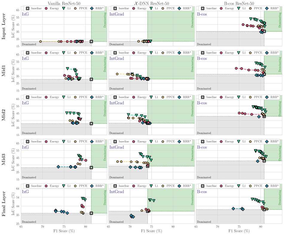
Fig. X8: Intermediate layer results comparing IoU vs. F1. We compare the effectiveness of model guidance at varying network depths (rows) for each attribution method and model (columns) across localization loss functions. We find similar trends across all configurations, with the $L_{1}$ loss outperforming all other losses. For the Vanilla and $\mathcal{X}$-DNN models, we observe improved performance across losses when optimizing at deeper layers of the network, whereas the results seem very stable for the B-cos models. For EPG results, see Fig. X7.

In Fig. B5, we show results for performing model guidance at additional intermediate layers: Mid1, Mid2, and Mid3. Specifically, for the ResNet-50 models we use, these layers correspond to the outputs of conv2_x, conv3_x, and conv4_x respectively in the ResNet nomenclature (he2016deep_2), while the final layer corresponds to the output of conv5_x. We find that the EPG performance at these intermediate layers through the network follows the trends when moving from the input to the final layer. Similar results for IoU can be found in Fig. X8.

EPG results for intermediate layers on VOC.

Fig. B5: Intermediate layer results comparing EPG vs. F1. We compare the effectiveness of model guidance at varying network depths (rows) for each attribution method and model (columns) across localization loss functions. For the B-cos model, we find similar trends at all network depths, with the Energy localization loss outperforming all other losses. For the Vanilla and $\mathcal{X}$-DNN models, the Energy loss similarly performs the best, but we also observe improved performance across losses when optimizing at deeper layers of the network. Full results can be found in Figs. X7 and X8.

B.4 Evaluating On-Object Localization

Evaluating on-object localization within bounding boxes.

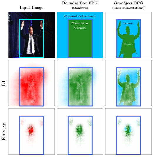
(a) Evaluating on-object localization within the bounding boxes: On-object EPG. In the standard EPG metric (middle column), we compute the fraction of positive attributions within the bounding boxes. In other words, attributions within the bounding box (green region) positively impact the metric, while attributions outside (blue region) negatively impact it. Since bounding boxes are coarse annotations and often include background regions, the standard EPG does not evaluate how well attributions localize on-object features, e.g. the person in the figure. To measure this, we evaluate with an additional Segmentation EPG metric (right column), where we compute the fraction of positive attributions in the bounding box that lie within the segmentation mask of the object. Here, attributions within the segmentation mask (green region) positively impact the metric, and attributions outside the segmentation mask and inside the bounding box (blue region) negatively impact it. Note that attributions outside the bounding box have no effect on Segmentation EPG. As an example and to visualize qualitative differences between losses, in the bottom rows ($L_{1}$, Energy), we show attributions for a B-cos model guided at the input layer. As becomes clear, by employing a uniform prior on attributions within the bounding box, the $L_{1}$ loss is effectively optimized to fill the entire bounding box and thus to not only highlight on-object features. This can also be observed quantitatively, see e.g. Fig. 6(b), right column.

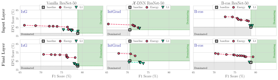
(b) On-object EPG results. We evaluate across models (columns) and layers (rows) for the Energy and $L_{1}$ localization losses. As seen qualitatively (e.g. Fig. 7), we find that the Energy loss is more effective than the $L_{1}$ loss in localizing attributions to the object as opposed to background regions within the bounding boxes. This is explained by the fact that the $L_{1}$ loss promotes uniformity in attributions within the bounding box, and treats both on-object and background features inside the box with equal importance, while the Energy loss only optimizes for attributions to lie within the bounding box without placing any constraints on where they may lie, leaving the model free to decide which regions within the box are important for its decision.

Fig. B6: Evaluating on-object localization via EPG. We show (a) the schema for the on-object EPG metric and how it differs the standard bounding box EPG metric, and (b) quantitative results on evaluating with on-object EPG.

The standard EPG metric (Eq. 2) evaluates the extent to which attributions localize to the bounding boxes. However, since such boxes often include background regions, the EPG score does not distinguish between attributions that focus on the object and attributions that focus on such background regions within the bounding boxes.

To additionally evaluate for on-object localization, we use a variant of EPG that we call On-object EPG. In contrast to standard EPG, we compute the fraction of positive attributions in pixels contained within the segmentation mask of the object out of positive attributions within the bounding box. This measures how well attributions within the bounding boxes localize to the object, and is not influenced by attributions outside the bounding boxes. A visual comparison of the two metrics is shown in Fig. B6.

We find that the Energy localization loss outperforms the $L_{1}$ localization loss both qualitatively (Fig. 6(a)) and quantitatively (Fig. 6(b)) on this metric. This is explained by the fact that the $L_{1}$ promotes uniformity in attributions across the bounding box, giving equal importance to on-object and background features within the box. In contrast, the Energy loss only optimizes for attributions to lie within the box, without any constraint on where in the box they lie. This also corroborates our previous qualitative observations (e.g. Fig. 7).

B.5 Model Guidance with Limited Annotations

Additional results for training with limited annotations

EPG score

IoU score

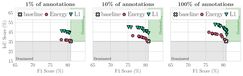
Fig. B8: EPG and IoU scores for limited annotations. We show EPG vs. F1 (left) and IoU vs. F1 (right) for B-cos attributions at the input when optimizing with the Energy and $L_{1}$ localization losses, when using $\{1\%,10\%,100\%\}$ training annotations. We find that model guidance is generally effective even when training with annotations for a limited number of images. While the performance slightly worsens when using 1% annotations, using just 10% annotated images yields similar gains to using a fully annotated training set. Full results can be found in Figs. X10 and X12.

In Fig. B8, we show the impact of using limited annotations when training (Sec. 5.4) when optimizing with the Energy and $L_{1}$ localization losses for B-cos attributions at the input. We find that in addition to EPG, trends in IoU scores also remain consistent even when using bounding boxes for just 1% of the the training images.

B.6 Model Guidance with Noisy Annotations

Additional results for training with coarse bounding boxes

(a) Vanilla ResNet-50 @ Final.

(b) $\mathcal{X}$-DNN ResNet-50 @ Final.

Fig. B9: Coarse bounding box results. We show the impact of dilating bounding boxes during training for the (a) Vanilla and (b) $\mathcal{X}$-DNN models. Similar to the results seen with B-cos models (Fig. 8), we find that the Energy localization loss is generally robust to coarse annotations, while the effectiveness of guidance with the $L_{1}$ localization loss worsens as the extent of coarseness (dilations) increases. Full results in Fig. X13.

In Fig. B9, we additionally show the impact of training with coarse, dilated bounding boxes for IxG attributions on the Vanilla model, and IntGrad attributions on the $\mathcal{X}$-DNN model. Similar to the results seen with B-cos attributions (Fig. 8), we find that the Energy localization loss is robust to coarse annotations, while the performance with $L_{1}$ localization loss worsens as the dilations increase.

Appendix C Waterbirds Results

				Conventional Setting					Reversed Setting
	Layer	Loss	G1 Acc	G2 Acc	G3 Acc	G4 Acc	Overall	G1 Acc	G2 Acc	G3 Acc	G4 Acc	Overall
0 B-cos 0	0Input0	Energy	99.2 ($\pm$0.1)	40.4 ($\pm$1.0)	56.1 ($\pm$4.0)	96.6 ($\pm$0.4)	71.2 ($\pm$0.1)	99.4 ($\pm$0.1)	70.2 ($\pm$2.1)	62.8 ($\pm$2.1)	96.5 ($\pm$0.6)	83.6 ($\pm$1.1)
		L1	99.3 ($\pm$0.1)	37.0 ($\pm$0.8)	51.1 ($\pm$1.9)	97.2 ($\pm$0.3)	69.5 ($\pm$0.2)	99.3 ($\pm$0.3)	67.7 ($\pm$3.3)	58.8 ($\pm$5.0)	96.7 ($\pm$0.7)	82.2 ($\pm$0.9)
	0Final0	Energy	99.3 ($\pm$0.1)	41.0 ($\pm$2.1)	53.1 ($\pm$0.8)	96.3 ($\pm$0.5)	71.1 ($\pm$0.9)	99.4 ($\pm$0.2)	70.1 ($\pm$3.1)	60.2 ($\pm$3.9)	95.8 ($\pm$1.1)	83.2 ($\pm$1.1)
		L1	99.3 ($\pm$0.1)	34.3 ($\pm$3.2)	49.4 ($\pm$2.6)	96.6 ($\pm$0.6)	68.2 ($\pm$1.1)	99.4 ($\pm$0.1)	69.8 ($\pm$2.1)	56.3 ($\pm$1.8)	96.1 ($\pm$0.7)	82.8 ($\pm$0.8)
lightgrey	Baseline		99.4 ($\pm$0.1)	37.2 ($\pm$0.2)	43.4 ($\pm$2.4)	96.5 ($\pm$0.1)	68.7 ($\pm$0.2)	99.4 ($\pm$0.1)	62.8 ($\pm$0.2)	56.6 ($\pm$2.4)	96.5 ($\pm$0.1)	80.1 ($\pm$0.2)
0 $\mathcal{X}$-DNN 0	0Input0	Energy	99.3 ($\pm$0.2)	47.0 ($\pm$9.1)	49.2 ($\pm$4.8)	96.8 ($\pm$0.7)	73.1 ($\pm$3.4)	99.0 ($\pm$0.3)	67.6 ($\pm$4.8)	63.9 ($\pm$3.6)	96.1 ($\pm$0.7)	82.6 ($\pm$2.0)
		L1	99.1 ($\pm$0.6)	40.4 ($\pm$7.3)	41.8 ($\pm$3.8)	96.5 ($\pm$0.6)	69.6 ($\pm$3.2)	99.3 ($\pm$0.2)	59.1 ($\pm$4.7)	63.6 ($\pm$6.1)	96.0 ($\pm$0.9)	79.3 ($\pm$1.3)
	0Final0	Energy	99.2 ($\pm$0.4)	42.5 ($\pm$10.4)	54.2 ($\pm$3.2)	96.6 ($\pm$0.9)	71.9 ($\pm$4.2)	99.2 ($\pm$0.2)	65.3 ($\pm$2.0)	62.3 ($\pm$3.3)	96.0 ($\pm$0.5)	81.5 ($\pm$0.9)
		L1	99.4 ($\pm$0.1)	45.1 ($\pm$4.0)	42.8 ($\pm$2.8)	96.5 ($\pm$0.5)	71.7 ($\pm$1.4)	99.3 ($\pm$0.2)	62.9 ($\pm$4.8)	59.8 ($\pm$4.8)	95.8 ($\pm$0.7)	80.4 ($\pm$1.8)
lightgrey	Baseline		99.3 ($\pm$0.1)	39.8 ($\pm$0.7)	38.6 ($\pm$2.5)	96.3 ($\pm$0.7)	69.1 ($\pm$0.6)	99.3 ($\pm$0.1)	60.2 ($\pm$0.7)	61.4 ($\pm$2.5)	96.3 ($\pm$0.7)	79.6 ($\pm$0.5)
0 Vanilla 0	0Input0	Energy	99.4 ($\pm$0.2)	42.4 ($\pm$2.6)	47.9 ($\pm$3.5)	97.1 ($\pm$0.4)	71.2 ($\pm$1.0)	99.6 ($\pm$0.2)	50.7 ($\pm$7.3)	52.4 ($\pm$1.7)	97.2 ($\pm$0.5)	75.1 ($\pm$2.9)
		L1	99.5 ($\pm$0.1)	46.1 ($\pm$4.4)	51.1 ($\pm$4.0)	97.5 ($\pm$0.1)	73.1 ($\pm$1.6)	99.6 ($\pm$0.1)	48.0 ($\pm$7.8)	49.7 ($\pm$3.7)	96.8 ($\pm$0.6)	73.7 ($\pm$2.7)
	0Final0	Energy	99.5 ($\pm$0.0)	56.1 ($\pm$7.0)	60.7 ($\pm$5.5)	97.0 ($\pm$0.5)	78.1 ($\pm$2.6)	99.5 ($\pm$0.1)	59.4 ($\pm$5.9)	56.5 ($\pm$3.7)	97.2 ($\pm$0.5)	78.9 ($\pm$1.9)
		L1	99.5 ($\pm$0.1)	57.1 ($\pm$2.9)	55.4 ($\pm$2.5)	96.7 ($\pm$0.6)	77.8 ($\pm$1.0)	99.5 ($\pm$0.1)	56.3 ($\pm$6.7)	51.6 ($\pm$3.1)	97.3 ($\pm$0.6)	77.1 ($\pm$2.5)
lightgrey	Baseline		99.4 ($\pm$0.0)	39.6 ($\pm$0.7)	53.7 ($\pm$2.1)	97.7 ($\pm$0.0)	70.8 ($\pm$0.0)	99.4 ($\pm$0.0)	60.4 ($\pm$0.7)	46.3 ($\pm$2.1)	97.7 ($\pm$0.0)	78.1 ($\pm$0.1)

Table C1: Classification performance on Waterbirds after model guidance with the $L_{1}$ and the Energy loss. We find that both losses consistently improve the models’ classification performance over the baseline model (i.e. a model without guidance). These improvements are particularly pronounced in the groups not seen during training, i.e. landbirds on water (“G2”) and waterbirds on land (“G3”). For qualitative visualizations of the effect of model guidance on the waterbirds dataset, see Fig. C1.

As discussed in section Sec. 5.5, we use the Waterbirds-100 dataset sagawa2019distributionally,petryk2022guiding_2 to evaluate the effectiveness of model guidance in a setting where strong spurious correlations are present in the training data. This dataset consists of four groups—Landbird on Land (G1), Landbird on Water (G2), Waterbird on Land (G3), and Waterbird on Water (G4)—of which only groups G1 and G4 appear during training and the background is thus perfectly correlated with the type of bird (e.g. Landbird on land).

To evaluate the effectiveness of model guidance, we train the models on two binary classification tasks: to classify the type of birds (the conventional setting) or the background (the reversed setting, as described in petryk2022guiding_2) and evaluate models without guidance (baselines), as well as with guidance: specifically, for guiding the models, we evaluate different models (Vanilla, $\mathcal{X}$-DNN, B-cos) with different guidance losses (Energy, $L_{1}$) applied at different layers (Input and Final), see Tab. C1. For each model, we use its corresponding attribution method, i.e. IxG for Vanilla, IntGrad for $\mathcal{X}$-DNN, and B-cos for B-cos.

In Tab. C1 we present the classification performance for the individual groups (G1-G4) as well as the average over all samples (‘Overall’) across all configurations; note that the group sizes differ in the test set and the average over the individual group acccuracies thus differs from the overall accuracy. For each row, the results are averaged over 4 runs (2 random training seeds and 2 different sets of 1% annotated samples) with the exception of the baseline results being an average over 2 runs.

In almost all cases, we find that both of the evaluated losses (Energy, $L_{1}$) improve the models’ classification performance over the baseline. As expected, these improvements are particularly pronounced in the groups not seen during training, i.e. landbirds on water (G2) and waterbirds on land (G3).

Further, in Fig. C1, we show attribution maps of the baseline models, as well as the guided models. As can be seen, model guidance not only improves the accuracy, but is also reflected in the attribution maps: e.g., in row 1 of Fig. 1(a), we see that while the baseline model originally focused on the background (water) to classify the image, it is possible to guide the model to use the desired features (i.e. the bird in conventional setting and the background in the reversed setting) and consequently arrive at the desired classification decision. As this guidance is ‘soft’, we also observe cases in which the model still focused on the wrong feature and thus arrived at the wrong prediction: e.g. in Fig. 1(b) row 1 (reversed setting), the Energy-guided model still focuses on the bird and thus incorrectly predicts ‘Water’, similar to the $L_{1}$-guided model in row 4.

Additional qualitative results on the Waterbirds-100 dataset.

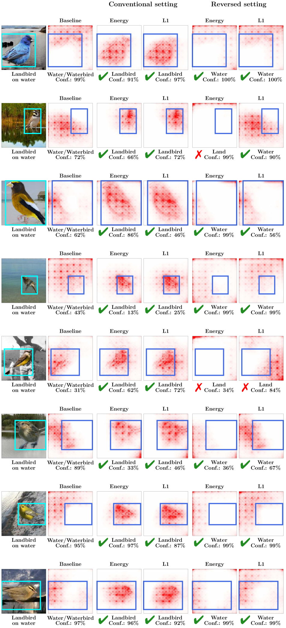
(a) Landbirds on Water.

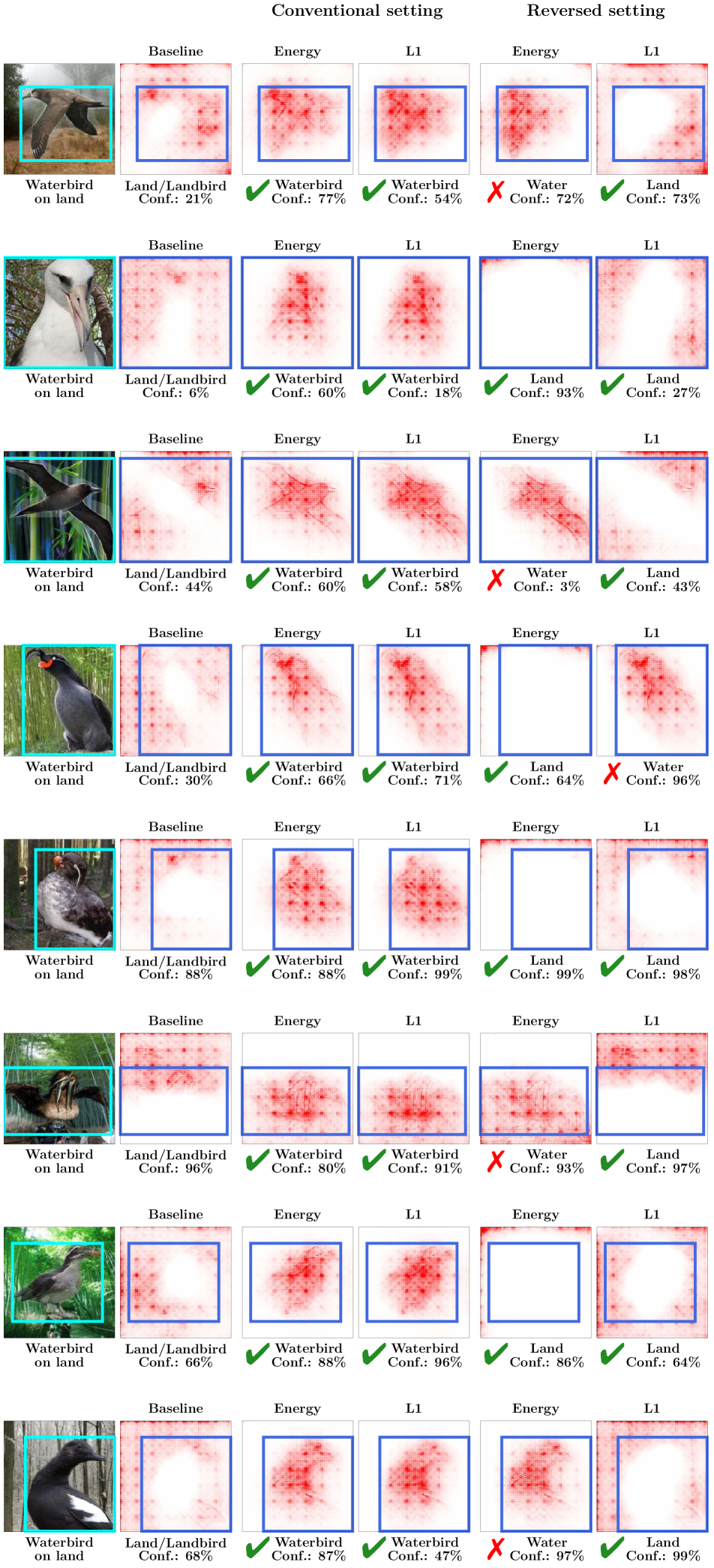
(b) Waterbirds on Land.

Fig. C1: Qualitative results for the Waterbirds dataset. Specifically, we show input layer attributions for B-cos models trained without guidance (‘Baseline’) as well as guided via the Energy or $L_{1}$ loss. We find that model guidance can be effective both for focusing on the bird and the background. For example, in the top row of (a), the model originally focuses on the background (col. 2) and classifies the image (col. 1) as Water/Waterbird. In the conventional setting, both the Energy and $L_{1}$ localization losses are effective in redirecting the focus to the bird (cols. 3-4), changing the model’s prediction to Landbird with high confidence. Similarly, in the reversed setting, both localization losses direct the focus to the background (cols. 5-6), which increases the model’s confidence in classifying the image as Water.

Appendix D Implementation Details

D.1 Training and Evaluation Details

Implementations: We implement our code using PyTorch paszke2019pytorch_2. The PASCAL VOC 2007 everingham2009pascal_2 and MS COCO 2014 lin2014microsoft_2 datasets and the Vanilla ResNet-50 model were obtained from the Torchvision library paszke2019pytorch_2,torchvision2016_2. Official implementations were used for the B-cos bohle2022b_2 and $\mathcal{X}$-DNN hesse2021fast_2 networks. Some of the utilities for data loading and evaluation were derived from NN-Explainer stalder2022wyswyc_2, and for visualization from the Captum library kokhlikyan2020captum_2.

D.1.1 Experiments with VOC and COCO

Training baseline models: We train starting from models pre-trained on ImageNet imagenet_2. We fine-tune with fixed learning rates in $\{10^{-3},10^{-4},10^{-5}\}$ using an Adam optimizer kingma2014adam_2 and select the checkpoint with the best validation F1-score. For VOC, we train for 300 epochs, and for COCO, we train for 60 epochs.

Training guided models: We train the models jointly optimized for classification and localization (Eq. 1) by fine-tuning the baseline models. We use a fixed learning rate of $10^{-4}$ and a batch size of $64$. For each configuration (given by a combination of attribution method, localization loss, and layer), we train using three different values of $\lambda_{\text{loc}}$, as detailed in Tab. D1. For VOC, we train for 50 epochs, and for COCO, we train for 10 epochs.

Selecting models to visualize: As described in Sec. 4, we select and evaluate on the set of Pareto-dominant models for each configuration after training. Each model on the Pareto front represents the extent of trade-off made between classification (F1) and localization (EPG) performance. In practice, the ‘best’ model to choose would depend on the requirements of the end user. However, to evaluate the effectiveness of model guidance (e.g. Figs. 1, 2 and 7), we select a representative model on the front whose attributions we visualize. This is done by selecting the model with the highest EPG score with an at most 5 p.p. drop in F1-score.

Efficient Optimization: As described in Sec. 3.5, for each image in a batch, we optimize for localization of a single class selected at random. This approximation allows us to perform model guidance efficiently and keeps the training cost tractable. However, to accurately evaluate the impact of this optimization, we evaluate the localization of all classes in the image at test time.

Training with Limited Annotations: As described in Sec. 5.4, we show that training with a limited number of annotations can be a cost effective way of performing model guidance. In order to maintain the relative magnitude of $\mathcal{L}_{\text{loc}}$ as compared to $\mathcal{L}_{\text{class}}$ in this setting, we scale up the values of $\lambda_{\text{loc}}$ when training. The values of $\lambda_{\text{loc}}$ we use are shown in Tab. D2.

D.1.2 Experiments with Waterbirds-100

Data distributions: The conventional binary classification task includes classifying Landbird from Waterbird, irrespective of their backgrounds. We use the same splits generated and published by petryk2022guiding_2. As discussed in Sec. C, at training time there are no samples from G2 or G3, making the bird type and the background perfectly correlated. In contrast, both the validation and test sets are balanced across foregrounds and backgrounds, i.e. a landbird is equally likely to occur on land or water, and vice-versa. However, as noted by sagawa2019distributionally_2, using a validation set with the same distribution as the test set leaks information on the test distribution in the process of hyperparameter and checkpoint selection during training. Therefore, we modify the validation split to avoid such information leakage; in particular, we use a validation set with the same distribution as the training set, and only use examples of groups G1 and G4. Note that Tab. 1 refers to G3 as the “Worst Group”.

Training details: We train starting from models pre-trained on ImageNet imagenet_2. We fine-tune with fixed learning rate of $10^{-5}$ with $\lambda_{\text{loc}}$ of $5\times 10^{-2}$ ($5\times 10^{-4}\times 100$ for using 1% of annotations) using an Adam optimizer kingma2014adam_2 . We train for 350 epochs with random cropping and horizontal flipping and select the checkpoint with the highest accuracy on the modified validation set.

Localization Loss	Values of $\lambda_{\text{loc}}$
Energy	$5\mkern 1.25mu{\times}\mkern 1.25mu10^{-4}$, 0 $1\mkern 1.25mu{\times}\mkern 1.25mu10^{-3}$, 0 $5\mkern 1.25mu{\times}\mkern 1.25mu10^{-3}$
$L_{1}$	$1\mkern 1.25mu{\times}\mkern 1.25mu10^{-3}$, 0 $5\mkern 1.25mu{\times}\mkern 1.25mu10^{-3}$, 0 $1\mkern 1.25mu{\times}\mkern 1.25mu10^{-2}$
PPCE	$1\mkern 1.25mu{\times}\mkern 1.25mu10^{-4}$, 0 $5\mkern 1.25mu{\times}\mkern 1.25mu10^{-4}$, 0 $1\mkern 1.25mu{\times}\mkern 1.25mu10^{-3}$
RRR*	$5\mkern 1.25mu{\times}\mkern 1.25mu10^{-6}$, 0 $1\mkern 1.25mu{\times}\mkern 1.25mu10^{-5}$, 0 $5\mkern 1.25mu{\times}\mkern 1.25mu10^{-5}$

Table D1: Hyperparameter $\lambda_{\text{loc}}$: Default training. used for when training on VOC and COCO with each localization loss. Different values are used for different loss functions since the magnitudes of each loss varies.

Localization Loss	Values of $\lambda_{\text{loc}}$
Energy	$0.05$, 0 $0.100$, 0 $0.50$
$L_{1}$	$0.01$, 0 $0.100$, 0 $1.00$

Table D2: Hyperparameter $\lambda_{\text{loc}}$: Limited annotations. used for when training on VOC and COCO with limited data for each localization loss. Different values are used for different loss functions since the magnitudes of each loss varies. We use larger values of $\lambda_{\text{loc}}$ when training with limited annotations to maintain the relative magnitudes of the classification and localization losses during training.

D.2 Optimizing B-cos Attributions

Training for optimizing the localization of attributions (Eq. 1) requires backpropagating through the attribution maps, which implies that they need to be differentiable. While B-cos attributions bohle2022b_2 as formulated are mathematically differentiable, the original implementation bohle2022b_2 for computing them involves detaching the dynamic weights from the computational graph, which prevents them from being used for optimization. In this work, to use them for model guidance, we develop a twice-differentiable implementation of B-cos attributions, the code for which can be found along with this supplement.

Appendix X Full Results

Full results on PASCAL VOC 2007 (F1 score).

Full results on MS COCO 2014 (F1 score).

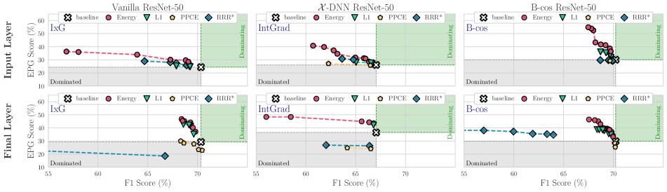
(a) EPG vs. F1.

(b) IoU vs. F1.

Fig. X2: EPG (a) and IoU (b) vs. F1 on COCO, for different losses (markers) and models (columns), optimized at different layers (rows); additionally, we show the performance of the baseline model before fine-tuning and demarcate regions that strictly dominate (are strictly dominated by) the baseline performance in green (grey). For each configuration, we show the Pareto fronts (cf. Fig. 4) across regularization strengths $\lambda_{\text{loc}}$ and epochs (cf. Sec. 5 and Fig. 4). We find the Energy loss to give the best trade-off between EPG and F1, whereas the $L_{1}$ loss (especially at the final layer) provides the best trade-off between IoU and F1. We further find these results to be consistent across datasets, see Fig. X1.

Mean Average Precision (mAP) results on VOC.

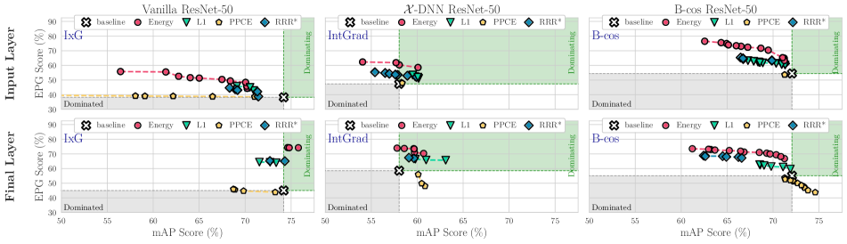
(a) EPG vs. mAP.

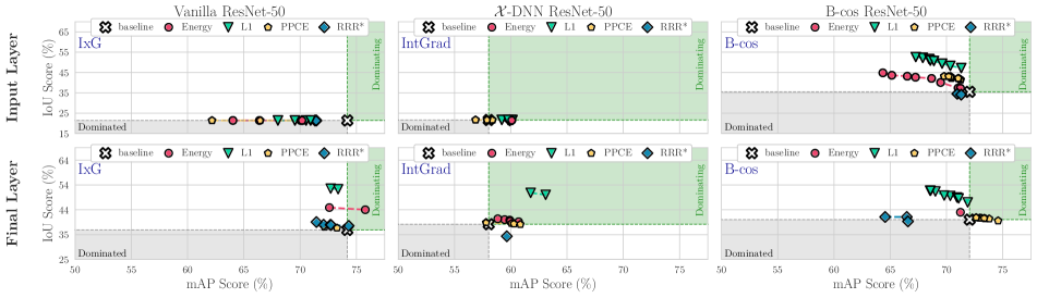
(b) IoU vs. mAP.

Fig. X3: Quantitative comparison of EPG and IoU vs. mAP scores for VOC. To ensure that the trends observed and described in the main paper generalize beyond the F1 metric, in this figure we show the EPG and IoU scores plotted against the mAP metric. In general, we find the results obtained for the mAP metric to be highly consistent with the previously shown results for the F1 metric, see Fig. X1. E.g., across all configurations, we find the Energy to yield the highest gains in EPG score, whereas the $L_{1}$ loss provides the best trade-offs with respect to the IoU metric. These results are further also consistent with those observed on COCO, see Fig. X4.

Full results on MS COCO 2014 (mAP).

(a) EPG vs. mAP.

(b) IoU vs. mAP.

Fig. X4: Quantitative comparison of EPG and IoU vs. mAP scores for COCO. To ensure that the trends observed and described in the main paper generalize beyond the F1 metric, in this figure we show the EPG and IoU scores plotted against the mAP metric. In general, we find the results obtained for the mAP metric to be highly consistent with the previously shown results for the F1 metric, see Fig. X2. E.g., across all configurations, we find the Energy to yield the highest gains in EPG score, whereas the $L_{1}$ loss provides the best trade-offs with respect to the IoU metric. These results are further also consistent with those observed on VOC, see Fig. X3.

Comparison to GradCAM on VOC.

(a) EPG vs. F1.

Comparison to GradCAM on COCO.

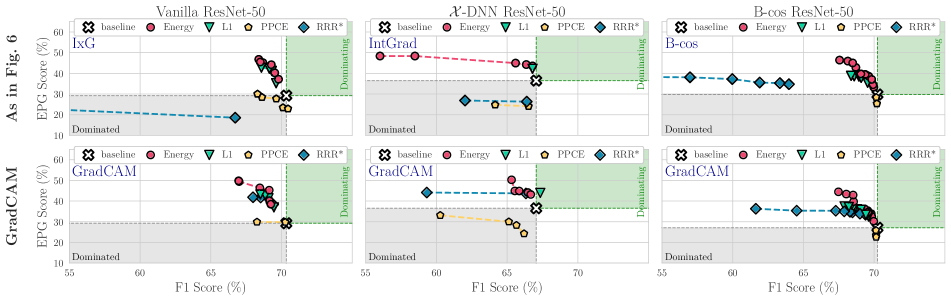
(a) EPG vs. F1.

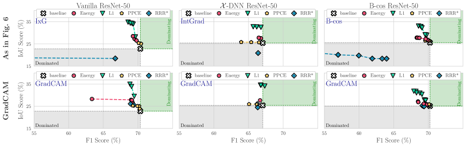
(b) IoU vs. F1.

Fig. X6: Quantitative results using GradCAM on COCO. We show EPG (a) and IoU (b) scores vs. F1 scores for all localization losses and models using GradCAM at the final layer (bottom rows in (a)+(b) and compare it to the results shown in the main paper (top rows). As expected, GradCAM performs very similarly to IxG (Vanilla) and IntGrad ($\mathcal{X}$-DNN) used at the final layer—in particular, note that for ResNet-50 architectures, IxG and IntGrad are very similar to GradCAM for Vanilla and $\mathcal{X}$-DNN models respectively (see Sec. B.2). Similarly, we find GradCAM to also perform comparably to the B-cos explanations when used at the final layer; for results on VOC, see Fig. X5.

EPG results for intermediate layers on VOC.

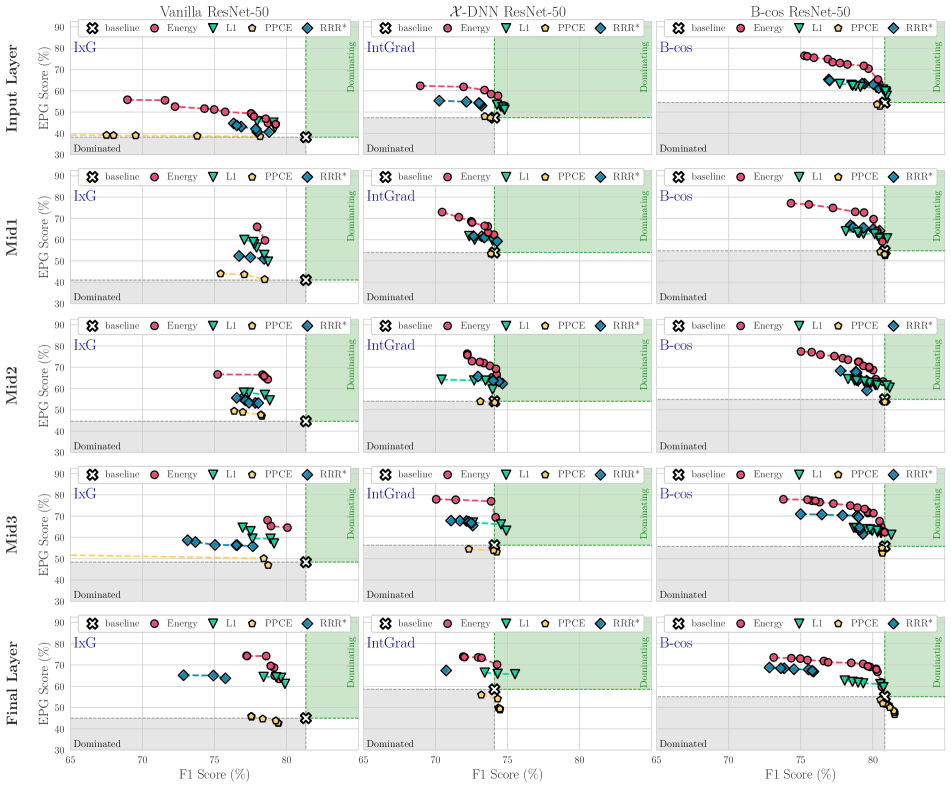
Fig. X7: Intermediate layer results comparing EPG vs. F1. We compare the effectiveness of model guidance at varying network depths (rows) for each attribution method and model (columns) across localization loss functions. For the B-cos model, we find similar trends at all network depths, with the Energy localization loss outperforming all other losses. For the Vanilla and $\mathcal{X}$-DNN models, the Energy loss similarly performs the best, but we also observe improved performance across losses when optimizing at deeper layers of the network. Results for IoU can be found in Fig. X8.

IoU results for intermediate layers on VOC.

Limited annotations — Input layer

EPG score

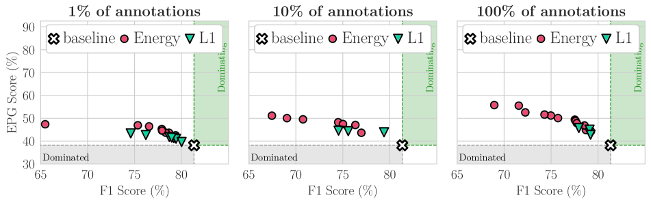
IoU score

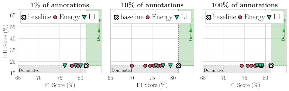
(a) Vanilla ResNet-50

EPG score

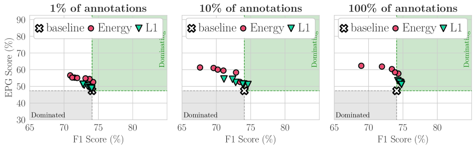
IoU score

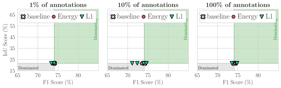
(b) $\mathcal{X}$-DNN ResNet-50

EPG score

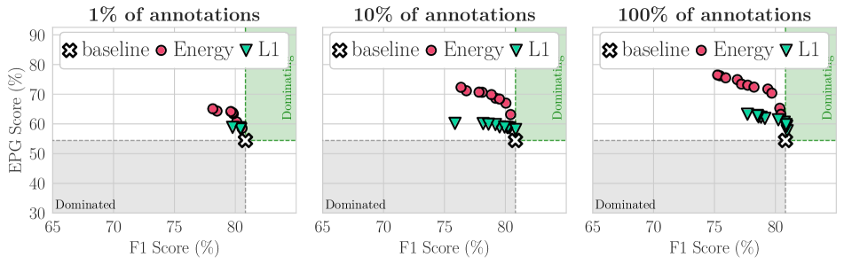
IoU score

(c) B-cos ResNet-50

Fig. X10: EPG and IoU scores for model guidance at the input layer with a limited number of annotations. We show EPG vs. F1 (left) and IoU vs. F1 (right) for all models, optimized with the Energy and $L_{1}$ localization losses, when using $\{1\%,10\%,100\%\}$ training annotations. We find that model guidance is generally effective even when training with annotations for a limited number of images. While the performance slightly worsens when using 1% annotations, using just 10% annotated images yields similar gains to using a fully annotated training set. Results at the final layer can be found in Fig. X12.

Limited annotations — Final layer

EPG score

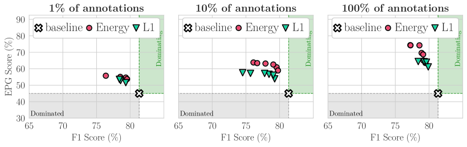
IoU score

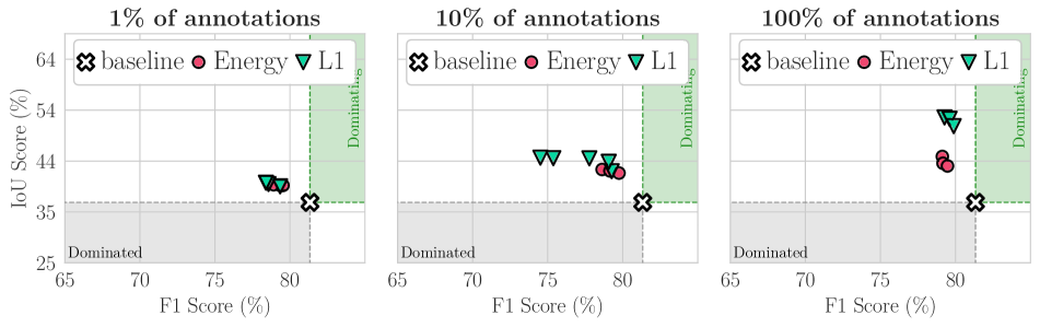
(a) Vanilla ResNet-50

EPG score

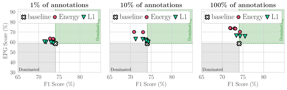
IoU score

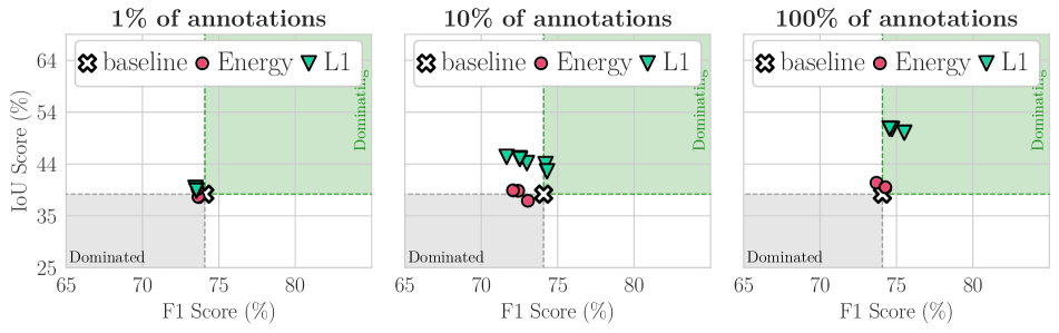
(b) $\mathcal{X}$-DNN ResNet-50

EPG score

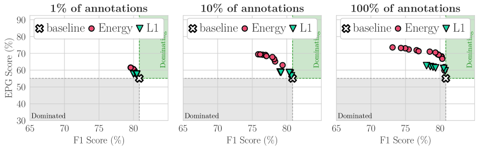
IoU score

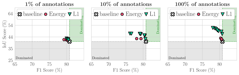
(c) B-cos ResNet-50

Fig. X12: EPG and IoU scores for model guidance at the final layer with a limited number of annotations. We show EPG vs. F1 (left) and IoU vs. F1 (right) for all models, optimized with the Energy and $L_{1}$ localization losses, when using $\{1\%,10\%,100\%\}$ training annotations. We find that model guidance is generally effective even when training with annotations for a limited number of images. While the performance worsens when using 1% annotations, using just 10% annotated images yields similar gains to using a fully annotated training set. Results at the input layer can be found in Fig. X10.

Additional results for training with coarse bounding boxes

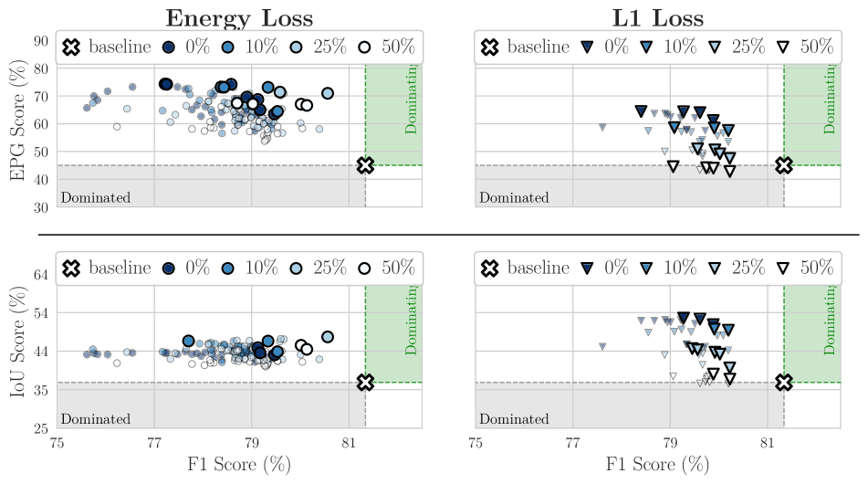
(a) Vanilla ResNet-50 @ Final.

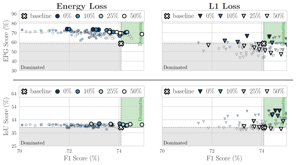
(b) $\mathcal{X}$-DNN ResNet-50 @ Final.

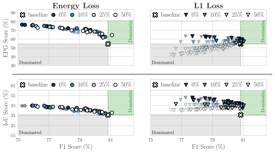
(c) B-cos ResNet-50 @ Input.

Fig. X13: Coarse bounding box results. We show the impact of dilating bounding boxes during training for the (a) Vanilla and (b) $\mathcal{X}$-DNN, and (c) B-cos models. Similar to the results seen with B-cos models (c), we find that the Energy localization loss is generally robust to coarse annotations, while the effectiveness of guidance with the $L_{1}$ localization loss worsens as the extent of coarseness increases.

ieee_fullname references_supp

References

- [1] Julius Adebayo, Justin Gilmer, Michael Muelly, Ian Goodfellow, Moritz Hardt, and Been Kim. Sanity Checks for Saliency Maps. In NeurIPS, 2018.
- [2] Julius Adebayo, Michael Muelly, Harold Abelson, and Been Kim. Post hoc Explanations may be Ineffective for Detecting Unknown Spurious Correlation. In ICLR, 2022.
- [3] Saeid Asgari, Aliasghar Khani, Fereshte Khani, Ali Gholami, Linh Tran, Ali Mahdavi-Amiri, and Ghassan Hamarneh. MaskTune: Mitigating Spurious Correlations by Forcing to Explore. In NeurIPS, 2022.
- [4] Sebastian Bach, Alexander Binder, Grégoire Montavon, Frederick Klauschen, Klaus-Robert Müller, and Wojciech Samek. On Pixel-Wise Explanations for Non-Linear Classifier Decisions by Layer-Wise Relevance Propagation. PLOS One, 10(7):e0130140, 2015.
- [5] Jürgen Backhaus. The Pareto Principle. Analyse & Kritik, 2(2):146–171, 1980.
- [6] Moritz Böhle, Mario Fritz, and Bernt Schiele. B-Cos Networks: Alignment is All We Need for Interpretability. In CVPR, pages 10329–10338, 2022.
- [7] Moritz Böhle, Mario Fritz, and Bernt Schiele. Convolutional Dynamic Alignment Networks for Interpretable Classifications. In CVPR, pages 10029–10038, 2021.
- [8] Aditya Chattopadhyay, Anirban Sarkar, Prantik Howlader, and Vineeth N Balasubramanian. Grad-CAM++: Improved Visual Explanations for Deep Convolutional Networks. In WACV, pages 839–847, 2018.
- [9] Piotr Dabkowski and Yarin Gal. Real Time Image Saliency for Black Box Classifiers. In NeurIPS, 2017.
- [10] Saurabh Desai and Harish G. Ramaswamy. Ablation-CAM: Visual Explanations for Deep Convolutional Network via Gradient-free Localization. In WACV, pages 983–991, 2020.
- [11] Gabriel Erion, Joseph D Janizek, Pascal Sturmfels, Scott M Lundberg, and Su-In Lee. Improving Performance of Deep Learning Models with Axiomatic Attribution Priors and Expected Gradients. Nature Machine Intelligence, 3(7):620–631, 2021.
- [12] Mark Everingham, Luc Van Gool, Christopher KI Williams, John Winn, and Andrew Zisserman. The Pascal Visual Object Classes (VOC) Challenge. IJCV, 88:303–308, 2009.
- [13] Vitaly Feldman and Chiyuan Zhang. What Neural Networks Memorize and Why: Discovering the Long Tail via Influence Estimation. In NeurIPS, pages 2881–2891, 2020.
- [14] Patrick Fernandes, Marcos Treviso, Danish Pruthi, André FT Martins, and Graham Neubig. Learning to Scaffold: Optimizing Model Explanations for Teaching. arXiv preprint arXiv:2204.10810, 2022.
- [15] Ruth C Fong and Andrea Vedaldi. Interpretable Explanations of Black Boxes by Meaningful Perturbation. In ICCV, pages 3429–3437, 2017.
- [16] Felix Friedrich, Wolfgang Stammer, Patrick Schramowski, and Kristian Kersting. A Typology to Explore and Guide Explanatory Interactive Machine Learning. arXiv preprint arXiv:2203.03668, 2022.
- [17] Hiroshi Fukui, Tsubasa Hirakawa, Takayoshi Yamashita, and Hironobu Fujiyoshi. Attention Branch Network: Learning of Attention Mechanism for Visual Explanation. In CVPR, pages 10705–10714, 2019.
- [18] Yuyang Gao, Tong Steven Sun, Guangji Bai, Siyi Gu, Sungsoo Ray Hong, and Zhao Liang. RES: A Robust Framework for Guiding Visual Explanation. In KDD, pages 432–442, 2022.
- [19] Yuyang Gao, Tong Steven Sun, Liang Zhao, and Sungsoo Ray Hong. Aligning Eyes between Humans and Deep Neural Network through Interactive Attention Alignment. ACM HCI, 6(CSCW2):1–28, 2022.
- [20] Hao Guo, Kang Zheng, Xiaochuan Fan, Hongkai Yu, and Song Wang. Visual Attention Consistency under Image Transforms for Multi-Label Image Classification. In CVPR, pages 729–739, 2019.
- [21] Misgina Tsighe Hagos, Kathleen M Curran, and Brian Mac Namee. Identifying Spurious Correlations and Correcting them with an Explanation-based Learning. arXiv preprint arXiv:2211.08285, 2022.
- [22] Kaiming He, Xiangyu Zhang, Shaoqing Ren, and Jian Sun. Deep Residual Learning for Image Recognition. In CVPR, pages 770–778, 2016.
- [23] Robin Hesse, Simone Schaub-Meyer, and Stefan Roth. Fast Axiomatic Attribution for Neural Networks. In NeurIPS, pages 19513–19524, 2021.
- [24] Peng-Tao Jiang, Chang-Bin Zhang, Qibin Hou, Ming-Ming Cheng, and Yunchao Wei. LayerCAM: Exploring Hierarchical Class Activation Maps for Localization. IEEE TIP, 30:5875–5888, 2021.
- [25] Joon Sik Kim, Gregory Plumb, and Ameet Talwalkar. Sanity Simulations for Saliency Methods. In ICML, 2022.
- [26] Keisuke Kiritoshi, Ryosuke Tanno, and Tomonori Izumitani. L1-Norm Gradient Penalty for Noise Reduction of Attribution Maps. In CVPRW, pages 118–121, 2019.
- [27] Kunpeng Li, Ziyan Wu, Kuan-Chuan Peng, Jan Ernst, and Yun Fu. Tell Me Where to Look: Guided Attention Inference Network. In CVPR, pages 9215–9223, 2018.
- [28] Tsung-Yi Lin, Michael Maire, Serge Belongie, James Hays, Pietro Perona, Deva Ramanan, Piotr Dollár, and C Lawrence Zitnick. Microsoft COCO: Common Objects in Context. In ECCV, pages 740–755. Springer, 2014.
- [29] Drew Linsley, Dan Shiebler, Sven Eberhardt, and Thomas Serre. Learning What and Where to Attend. arXiv preprint arXiv:1805.08819, 2018.
- [30] Masahiro Mitsuhara, Hiroshi Fukui, Yusuke Sakashita, Takanori Ogata, Tsubasa Hirakawa, Takayoshi Yamashita, and Hironobu Fujiyoshi. Embedding Human Knowledge into Deep Neural Network via Attention Map. arXiv preprint arXiv:1905.03540, 2019.
- [31] Ofir Moshe, Gil Fidel, Ron Bitton, and Asaf Shabtai. Improving Interpretability via Regularization of Neural Activation Sensitivity. arXiv preprint arXiv:2211.08686, 2022.
- [32] Krishna Kanth Nakka and Mathieu Salzmann. Towards Robust Fine-Grained Recognition by Maximal Separation of Discriminative Features. In ACCV, 2020.
- [33] Vilfredo Pareto. Il massimo di utilità dato dalla libera concorrenza. Giornale degli economisti, pages 48–66, 1894.
- [34] Vilfredo Pareto. The Maximum of Utility given by Free Competition. Giornale degli Economisti e Annali di Economia, 67(3):387–403, 2008.
- [35] Suzanne Petryk, Lisa Dunlap, Keyan Nasseri, Joseph Gonzalez, Trevor Darrell, and Anna Rohrbach. On Guiding Visual Attention with Language Specification. In CVPR, pages 18092–18102, 2022.
- [36] Vitali Petsiuk, Abir Das, and Kate Saenko. RISE: Randomized Input Sampling for Explanation of Black-box Models. In BMVC, 2018.
- [37] Vipin Pillai, Soroush Abbasi Koohpayegani, Ashley Ouligian, Dennis Fong, and Hamed Pirsiavash. Consistent Explanations by Contrastive Learning. In CVPR, pages 10213–10222, 2022.
- [38] Vipin Pillai and Hamed Pirsiavash. Explainable Models with Consistent Interpretations. In AAAI, 2021.
- [39] Sukrut Rao, Moritz Böhle, and Bernt Schiele. Towards Better Understanding Attribution Methods. In CVPR, pages 10223–10232, 2022.
- [40] Marco Tulio Ribeiro, Sameer Singh, and Carlos Guestrin. “Why Should I Trust You?”: Explaining the Predictions of Any Classifier. In KDD, pages 1135–1144, 2016.
- [41] Laura Rieger, Chandan Singh, William Murdoch, and Bin Yu. Interpretations are Useful: Penalizing Explanations to Align Neural Networks with Prior Knowledge. In ICML, pages 8116–8126. PMLR, 2020.
- [42] Andrew Slavin Ross, Michael C Hughes, and Finale Doshi-Velez. Right for the Right Reasons: Training Differentiable Models by Constraining their Explanations. In IJCAI, pages 2662–2670, 2017.
- [43] Olga Russakovsky, Jia Deng, Hao Su, Jonathan Krause, Sanjeev Satheesh, Sean Ma, Zhiheng Huang, Andrej Karpathy, Aditya Khosla, Michael Bernstein, Alexander C. Berg, and Li Fei-Fei. ImageNet Large Scale Visual Recognition Challenge. IJCV, 115(3):211–252, 2015.
- [44] Shiori Sagawa, Pang Wei Koh, Tatsunori B Hashimoto, and Percy Liang. Distributionally Robust Neural Networks for Group Shifts: On the Importance of Regularization for Worst-Case Generalization. In ICLR, 2020.
- [45] Patrick Schramowski, Wolfgang Stammer, Stefano Teso, Anna Brugger, Franziska Herbert, Xiaoting Shao, Hans-Georg Luigs, Anne-Katrin Mahlein, and Kristian Kersting. Making Deep Neural Networks Right for the Right Scientific Reasons by Interacting with their Explanations. Nature Machine Intelligence, 2(8):476–486, 2020.
- [46] Ramprasaath R Selvaraju, Michael Cogswell, Abhishek Das, Ramakrishna Vedantam, Devi Parikh, and Dhruv Batra. Grad-CAM: Visual Explanations from Deep Networks via Gradient-Based Localization. In ICCV, pages 618–626, 2017.
- [47] Ramprasaath R Selvaraju, Stefan Lee, Yilin Shen, Hongxia Jin, Shalini Ghosh, Larry Heck, Dhruv Batra, and Devi Parikh. Taking a HINT: Leveraging Explanations to Make Vision and Language Models More Grounded. In ICCV, pages 2591–2600, 2019.
- [48] Xiaoting Shao, Arseny Skryagin, Wolfgang Stammer, Patrick Schramowski, and Kristian Kersting. Right for Better Reasons: Training Differentiable Models by Constraining their Influence Functions. In AAAI, volume 35, pages 9533–9540, 2021.
- [49] Haifeng Shen, Kewen Liao, Zhibin Liao, Job Doornberg, Maoying Qiao, Anton Van Den Hengel, and Johan W Verjans. Human-AI Interactive and Continuous Sensemaking: A Case Study of Image Classification using Scribble Attention Maps. In Extended Abstracts of CHI, pages 1–8, 2021.
- [50] Avanti Shrikumar, Peyton Greenside, and Anshul Kundaje. Learning Important Features Through Propagating Activation Differences. In ICML, pages 3145–3153, 2017.
- [51] Karen Simonyan, Andrea Vedaldi, and Andrew Zisserman. Deep Inside Convolutional Networks: Visualising Image Classification Models and Saliency Maps. In ICLRW, 2014.
- [52] Krishna Kumar Singh, Dhruv Mahajan, Kristen Grauman, Yong Jae Lee, Matt Feiszli, and Deepti Ghadiyaram. Don’t Judge an Object by its Context: Learning to Overcome Contextual Bias. In CVPR, pages 11070–11078, 2020.
- [53] Jost Tobias Springenberg, Alexey Dosovitskiy, Thomas Brox, and Martin Riedmiller. Striving for Simplicity: The All Convolutional Net. In ICLRW, 2015.
- [54] Guolei Sun, Salman Khan, Wen Li, Hisham Cholakkal, Fahad Shahbaz Khan, and Luc Van Gool. Fixing Localization Errors to Improve Image Classification. In ECCV, pages 271–287. Springer, 2020.
- [55] Mukund Sundararajan, Ankur Taly, and Qiqi Yan. Axiomatic Attribution for Deep Networks. In ICML, pages 3319–3328, 2017.
- [56] Damien Teney, Ehsan Abbasnedjad, and Anton van den Hengel. Learning What Makes a Difference from Counterfactual Examples and Gradient Supervision. In ECCV, pages 580–599. Springer, 2020.
- [57] Stefano Teso. Toward Faithful Explanatory Active Learning with Self-Explainable Neural Nets. In Workshop on IAL, pages 4–16. CEUR Workshop Proceedings, 2019.
- [58] Stefano Teso, Öznur Alkan, Wolfang Stammer, and Elizabeth Daly. Leveraging Explanations in Interactive Machine Learning: An Overview. arXiv preprint arXiv:2207.14526, 2022.
- [59] Stefano Teso and Kristian Kersting. Explanatory Interactive Machine Learning. In AIES, pages 239–245, 2019.
- [60] Haofan Wang, Zifan Wang, Mengnan Du, Fan Yang, Zijian Zhang, Sirui Ding, Piotr Mardziel, and Xia Hu. Score-CAM: Score-Weighted Visual Explanations for Convolutional Neural Networks. In CVPRW, pages 111–119, 2020.
- [61] Kai Yuanqing Xiao, Logan Engstrom, Andrew Ilyas, and Aleksander Madry. Noise or Signal: The Role of Image Backgrounds in Object Recognition. In ICLR, 2021.
- [62] Ziyan Yang, Kushal Kafle, Franck Dernoncourt, and Vicente Ordóñez Román. Improving Visual Grounding by Encouraging Consistent Gradient-based Explanations. arXiv preprint arXiv:2206.15462, 2022.
- [63] Matthew D Zeiler and Rob Fergus. Visualizing and Understanding Convolutional Networks. In ECCV, pages 818–833, 2014.
- [64] Michael Zhang, Nimit S Sohoni, Hongyang R Zhang, Chelsea Finn, and Christopher Ré. Correct-N-Contrast: A Contrastive Approach for Improving Robustness to Spurious Correlations. arXiv preprint arXiv:2203.01517, 2022.
- [65] Yilun Zhou, Serena Booth, Marco Tulio Ribeiro, and Julie Shah. Do Feature Attribution Methods Correctly Attribute Features? In AAAI, volume 36, pages 9623–9633, 2022.
Using Explanations To Guide Models