Effective one-band models for the 1D cuprate Ba_2-xSr_xCuO_3+δ

Abstract

We consider a multiband Hubbard model $H_{m}$ for Cu and O orbitals in Ba_2-xSr_xCuO_3+δ similar to the tree-band model for two-dimensional (2D) cuprates. The hopping parameters are obtained from maximally localized Wannier functions derived from ab initio calculations. Using the cell perturbation method, we derive both a generalized $t-J$ model $H_{tJ}$ and a one-band Hubbard model $H_{H}$ to describe the low-energy physics of the system. $H_{tJ}$ has the advantage of having a smaller relevant Hilbert space, facilitating numerical calculations, while additional terms should be included in $H_{H}$ to accurately describe the multi-band physics of $H_{m}$. Using $H_{tJ}$ and DMRG, we calculate the wave-vector resolved photoemission and discuss the relevant features in comparison with recent experiments. In agreement with previous calculations, we find that the addition of an attractive nearest-neighbor interaction of the order of the nearest-neighbor hopping shifts weight from the $3k_{F}$ to the holon-folding branch. Kinetic effects also contribute to this process.

I Introduction

After more than three decades from the discovery of high-$T_{c}$ superconductivity, the pairing mechanism is still not fully understood, although it is believed that it is related to spin fluctuations originating from the effective Cu-Cu superexchange $J$, and complicated by the existence of several phases competing with superconductivity Keimer et al. (2015); Fradkin et al. (2015); OḾahony et al. (2022); Dong et al. (2022). However, there is consensus that for energies below an energy scale of the order of 1 eV, the physics of the two-dimensional (2D) superconducting cuprates is described by the three-band Hubbard modelVarma et al. (1987); Emery (1987) $H_{3b}$, which contains the 3d${}_{x^{2}-y^{2}}$ orbitals of Cu and the 2p_σ orbitals of O .

More recently, one-dimensional (1D) cuprates have attracted a great deal of attention, in particular because numerical techniques in 1D are more powerful and also field-theoretical methods like bosonization can be used Neudert et al. (2000); Zaliznyak et al. (2004); Kim et al. (2006); Walters et al. (2009); Schlappa et al. (2012); Wohlfeld et al. (2013); Chen et al. (2021); Jin et al. (2021); Li et al. (2021a); Wang et al. (2021); Qu et al. (2022); Tang et al. (2022); Wang et al. (2022). Neudert et al. have studied experimentally and theoretically the distribution of holes in the 1D cuprate Sr₂CuO₃ Neudert et al. (2000). The authors discuss several multiband models and the effect of several terms. Recently, angle-resolved photoemission experiments have been carried out in a related doped compound Ba_2-xSr_xCuO_3+δ and analyzed on the basis of a one-band Hubbard model with parameters chosen ad hock Chen et al. (2021). The need to add nearest-neighbor attraction or phonons to fit the experiment has been suggested Chen et al. (2021); Wang et al. (2021); Tang et al. (2022); Wang et al. (2022). Li et al. studied a four-band and a one-band Hubbard model and noted that the latter lacks the electron-hole asymmetry observed in resonant inelastic x-ray scattering experiments Li et al. (2021a).

The questions we want to address in this work are: 1) which is the appropriate multiband Hubbard model $H_{m}$ to describe Ba_2-xSr_xCuO_3+δ? 2) What are the physical values of the parameters? 3) To what extent can this model be represented by simpler one-band ones?

Due to the large Hilbert space of $H_{m}$, different low-energy reduction procedures have been used to obtain simpler effective Hamiltonians for the 2D cuprates Schüttler and Fedro (1992); Simon et al. (1993); Simón and Aligia (1993); Feiner et al. (1996); Belinicher et al. (1994); Belinicher and Chernyshev (1994); Aligia et al. (1994). Most of them are based on projections of $H_{m}$ onto the low-energy space of Zhang-Rice singlets (ZRS) Zhang and Rice (1988). In spite of some controversy remaining about the validity of this approach Ebrahimnejad et al. (2014); Hamad et al. (2021); Adolphs et al. (2016); Hamad et al. (2018); Jiang et al. (2020); Aligia (2020), the resulting effective models seem to describe well the physics of the 2D cuprates. However, the effect of excited states above the ZRS, often neglected, can have an important roleLi et al. (2021b). For example, if one considers the Hubbard model as an approximation to $H_{m}$ (as done in Ref. Chen et al., 2021), it is known that it leads, in second-order in the hopping $t$, to a term which in one dimension (1D) takes the form

$$H_{t^{\prime\prime}}=t^{\prime\prime}\sum\limits_{i\sigma}\left(c_{i+2\bar{\sigma}}^{\dagger}c_{i+1\sigma}^{\dagger}c_{i+1\bar{\sigma}}c_{i\sigma}-c_{i+2\sigma}^{\dagger}n_{i+1\bar{\sigma}}c_{i\sigma}+\text{H.c.}\right),$$ (1)

with $t^{\prime\prime}=t^{2}/U>0$, where $n_{i\sigma}=c_{i\sigma}^{\dagger}c_{i\sigma}$ and $\bar{\sigma}=-\sigma.$ This term is an effective repulsion and inhibits superconductivity in 1D, while as expected, it favors superconductivity if the sign is changed Ammon et al. (1995); Lema et al. (1996). Interestingly, some derivations of the generalized $t-J$ model for 2D cuprates suggest that $t^{\prime\prime}$ can be negative for some parameters of $H_{m}$ Aligia et al. (1994); Simón and Aligia (1995), and a very small term $t^{\prime\prime}=-t/20$ can have a dramatic effect favoring $d$-wave superconductivity Batista et al. (1997). Even if the realistic $t^{\prime\prime}$ is positive, it is expected to be smaller than that derived from the Hubbard model and might explain why studies of the superconductivity in the one-band Hubbard model conclude that part of the pairing interaction is missingDong et al. (2022).

Therefore, a discussion on the appropriate model to describe the 1D cuprates and, in particular, Ba_2-xSr_xCuO_3+δ seems necessary. In this work we calculate the hopping parameters of the multiband model for this compound and use this information to derive simpler one-band models.

The paper is organized as follows. In Section II we explain the multiband Hubbard model $H_{m}$ and derive its hopping parameters using maximally localized Wannier functions (MLWF). In Section III we describe the resulting generalized $t-J$ model obtained from $H_{m}$ by a low-energy reduction procedure explained briefly in the appendix. In Section IV we explain the corresponding results for the one-band Hubbard model. In Section V we calculate the photoemission spectrum using the time-dependent density-matrix renormalization-group methodWhite and Feiguin (2004); Daley et al. (2004); Feiguin and White (2005); Paeckel et al. (2019) and we compare it with previous experimental and theoretical results. Section VI contains a summary and discussion.

II The multiband Hubbard model

We use the following form of the Hamiltonian

$$H_{m} = U_{d}\sum\limits_{i}d_{i\uparrow}^{\dagger}d_{i\uparrow}d_{i\downarrow}^{\dagger}d_{i\downarrow}+\sum\limits_{i\sigma}\{\epsilon_{\text{Cu}}d_{i\sigma}^{\dagger}d_{i\sigma}$$ (2)

$$+\frac{\epsilon_{\text{O}}}{2}\sum\limits_{\delta}p_{i+\delta\sigma}^{\dagger}p_{i+\delta\sigma}+\epsilon_{\text{O}}^{\text{ap}}\sum\limits_{\gamma}p_{i+\gamma\sigma}^{\dagger}p_{i+\gamma\sigma}$$

$$+[d_{i\sigma}^{\dagger}(t_{pd}^{x}\sum\limits_{\delta}p_{i+\delta\sigma}+t_{pd}^{y}\sum\limits_{\gamma}p_{i+\delta\gamma})$$

$$-t_{pp}\sum\limits_{\delta\gamma}p_{i+\delta\sigma}^{\dagger}p_{i+\gamma\sigma}+\text{H.c.}]\},$$

where $d_{i\sigma}^{\dagger}$ ($p_{j\sigma}^{\dagger}$) creates a hole with spin $\sigma$ at Cu (O) site $i$ ($j$). We choose the chain direction as $x$ ($a$ in Fig. 1) and $\delta=\pm a\mathbf{\hat{x}}/2$ denote the vectors that connect a Cu atom with their nearest O atoms in the chain direction, where $a$ is the Cu-Cu distance that we take as $1$ in what follows. $\gamma$ has a similar meaning for the apical O atoms, displaced from the chain in the $y$ direction ($c$ in Fig. 1). The relevant O orbitals are those pointing towards their nearest Cu atoms. To simplify the form of the Hamiltonian, we have changed the signs of half of the orbitals in such a way that sign of the hopping terms do not depend on direction and $t_{pd}^{x},t_{pd}^{y},t_{pp}>0$ .

In comparison with previous approaches Neudert et al. (2000); Li et al. (2021a), two terms are missing: the intratomic O repulsion $U_{p}$ and the interatomic Cu-O repulsion $U_{pd}$. Although the former is rather sizeable ($U_{p}\sim 4$ eV has been estimated in 2D cuprates Hybertsen et al. (1989)), we find that it has very little influence on the parameters of the one-band models because of the low probability of double hole occupancy at the O sites. The value of $U_{pd}$ is difficult to determine from spectroscopic measurements Sheshadri et al. (2023) and its effect on different quantities can be absorbed in other parameters Neudert et al. (2000). We obtain a better agreement with the measured photoemission spectra assuming $U_{pd}=0$. We also take $U_{d}=10$ eV and $\Delta=\epsilon_{\text{O}}-\epsilon_{\text{Cu}}=3.5$ eV, from calculations in the 2D cuprates Hybertsen et al. (1989) and $\epsilon_{\text{O}}^{\text{ap}}-\epsilon_{\text{O}}=-0.4$ eV was determined as the value that leads to a ratio 1.225 between the occupancy of apical and chain O atoms, very similar to determined experimentally in Sr₂CuO₃ Neudert et al. (2000). The values of the hopping parameters $t_{pd}^{x}=1.10$ eV, $t_{pd}^{y}=1.04$ eV, and $t_{pp}=0.60$ eV were determined from density functional theory (DFT) calculations along with the MLWF method.

For the DFT calculations, we use the QUANTUM ESPRESSO code Giannozzi et al. (2009, 2017), with the GGA approximation for the exchange and correlation potential and PAW-type pseudopotentials. The energy cut for the plane waves is 80 Ry, and the mesh used in reciprocal space is $15\times 15\times 5$. The unit cell is an orthorhombic structure with lattice parameters $a=3.85$Å, $b=4.17$Å  and $c=13.18$Å, and contains two formula units, see Fig. 1.

We consider the spin unpolarized case and obtain the bands shown in Fig. 2. The MLWF procedure involves band fitting of the DFT results, as shown in blue in Fig. 2. The energy window selected to project the Wannier orbital is between 3.75 eV and 10.75 eV, and the orbitals are centered in Cu and O atoms with $d$ and $p$ character, respectively. Other convergence parameters are also successfully evaluated, as suggested in Ref. Pizzi et al., 2020. Finally, the hopping parameters are extracted from the Hamiltonian expressed in the Wannier basis.

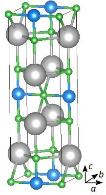
Figure 1: Unit cell of BaCuO₃. The gray/blue/green ball are Ba/Cu/O respectively. The lattice parameters are $a=3.85$Å, $b=4.17$Å  and $c=13.18$Å. The CuO chains are along the $a$ direction with distance among them of 4.14Å.

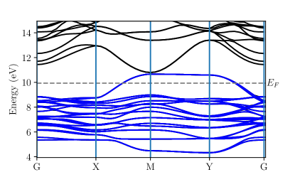
Figure 2: Band structure for the BaCuO₃ obtained for unpolarized DFT calculation. In blue the bands from the MLWF procedure superposed with DFT ones.

III The generalized $t-J$ model

Using the cell-perturbation method Feiner et al. (1996); Belinicher et al. (1994), with appropriate modifications for this 1D compound, we find that the system can be described with the following generalized $t-J$ model

$$H_{tJ} = -t\sum\limits_{i\sigma}\left(c_{i\sigma}^{\dagger}c_{i+1\sigma}+\text{H.c.}\right)$$ (3)

$$-t_{2}\sum\limits_{i\sigma}\left(c_{i\sigma}^{\dagger}c_{i+2\sigma}+\text{H.c.}\right)$$

$$+\sum\limits_{i}\left(J\mathbf{S}_{i}\cdot\mathbf{S}_{i+1}+Vn_{i}n_{i+1}\right)+H_{t^{\prime\prime}},$$

with $t_{2}=t/5$. Minor terms of magnitude below 0.04 eV were neglected. The parameters of the model are given by analytical expressions in terms of the eigenstates and energies of a cell Hamiltonian, that are obtained after solving a $6\times 6$ matrix and two $3\times 3$ matrices. A summary of the method is included in the appendix.

For the parameters of the multiband model described above, we obtain $t=0.443$ eV, $J=0.314$ eV, $V=-0.143$ eV, and $t^{\prime\prime}=0.068$ eV. Interestingly, our values for $J$ and $t^{\prime\prime}$ without adjustable parameters are similar to those corresponding to the Hubbard model chosen to explain the experiments by Chen et al. Chen et al. (2021).

The larger values of $t$ and $J$ compared to the 2D cuprates (for example $t=0.37$ meV, $J=0.15$ meV for T-CuO Hamad et al. (2018)) are expected due to the larger overlap between the normalized O orbitals $\sum\limits_{\delta}p_{i+\delta\sigma}$ that hybridize with the Cu for nearest-neighbor Cu positions. This leads to a larger overlap between non-orthogonal ZRS Aligia et al. (1994); Zhang (1989) and to a larger extension of the orthogonal oxygen Wannier functions centered at the Cu sites (see appendix). For Sr₂CuO₃, the reported values of $J\sim 0.24$ meV Neudert et al. (2000); Zaliznyak et al. (2004); Kim et al. (2006); Walters et al. (2009); Schlappa et al. (2012) are also larger than those of 2D cuprates. The resulting value of $t$ is somewhat smaller than that used in Ref. Chen et al., 2021 but is is compensated by the hopping to second nearest neighbors.

The fact that the nearest-neighbor attraction $V$ is larger than $J/4$ as expected for the mapping from the Hubbard to the $t-J$ model is due to the contribution of excited local triplets absent in the Hubbard model.

For other parameters of $H_{m}$, in particular increasing the ratio $t_{pp}/t_{pd}$ and the difference between O and Cu on-site energies, $t^{\prime\prime}$ changes sign as expected from calculations in 2D cuprates Aligia et al. (1994); Simón and Aligia (1995). For example increasing $t_{pp}$ to 1 eV and both on-site energy differences to 7 eV (unrealistic for Ba_2-xSr_xCuO_3+δ but near to the values expected for nickelates), we obtain $t=0.531$ eV, $J=0.105$ eV, $V=-0.096$ eV, and $t^{\prime\prime}=-0.019$ eV, due to the increasing relative importance of excited triplets.

IV The effective one-band Hubbard model

The generalized $t-J$ model discussed above describes the movement of ZRS (two-hole states) in a chain of singly occupied cells. If the cells with no holes are also considered (because for example one is interested in larger energy scales), one can also derive a one-band Hubbard-like model using the cell perturbation method. A simple version of this model has the form Schüttler and Fedro (1992); Simon et al. (1993); Simón and Aligia (1993)

$$H_{H} = -t\sum\limits_{i\sigma}\left(c_{i\sigma}^{\dagger}c_{i+1\sigma}+\text{H.c.}\right)[t_{AA}(1-n_{i\bar{\sigma}})(1-n_{i+1\bar{\sigma}})$$ (4)

$$+t_{BB}n_{i\bar{\sigma}}n_{i+1\bar{\sigma}}+t_{AB}(n_{i\bar{\sigma}}+n_{i+1\bar{\sigma}}-2n_{i\bar{\sigma}}n_{i+1\bar{\sigma}})]$$

$$+U\sum\limits_{i}n_{i\uparrow}n_{i\downarrow}.$$

As for $H_{tJ}$, we map the ZRS into empty states of $H_{H}$. Then $t_{AA}$ coincides with $t$ of $H_{tJ}$. From the mapping procedure we obtain $t_{AA}=0.443$ eV, $t_{AB}=0.421$ eV, $t_{BB}=0.369$ eV, and $U=2.083$ eV. The model is electron-hole symmetric if and only if $t_{AA}=t_{BB}$, while the photoemission of $H_{m}$ is asymmetric in general Li et al. (2021a).

Another shortcoming of $H_{H}$ is that if the model is reduced to a generalized $t-J$ one by eliminating double occupied sites, the effective $J=4t_{AB}^{2}/U=0.376$ eV and $t^{\prime\prime}=J/4=0.094$eV are overestimated with respect to the values obtained in the previous section: $J=0.314$ eV, and $t^{\prime\prime}=0.068$ eV. Instead, the NN attraction $-J/4$ is underestimated ($V=-0.143$ eV above). This is due to the neglect of the triplets in $H_{H}$ (see appendix and Ref. Simón and Aligia, 1995). Therefore $H_{tJ}$ is more realistic to describe the photoemission spectrum of hole doped 1D cuprates, unless additional terms are added to $H_{H}$.

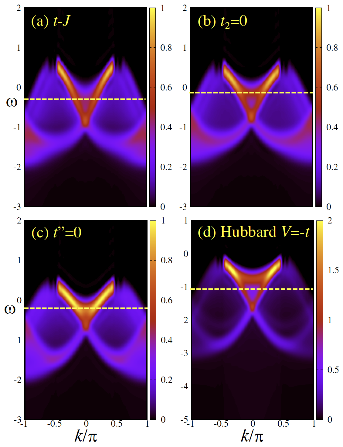
Figure 3: Photoemission spectrum of (a) the generalized $t-J$, Eq. 3; (b) same but setting the second-neighbor hopping to zero; (c) $t^{\prime\prime}=0$. Panel (d) shows results for the extended Hubbard model with $t=0.6,U/t=8;V/t=-1$ for comparison.

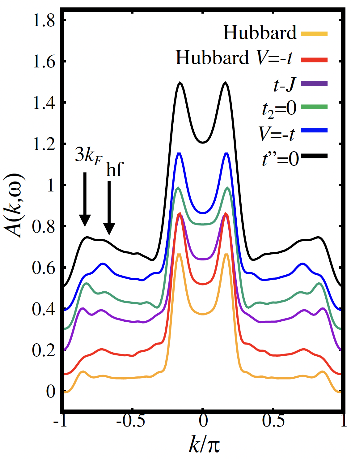
Figure 4: Momentum distribution curves: cuts along the fixed frequency dashed lines in Fig. 3. The features corresponding to the holon-folding (hf) and $3k_{F}$ bands are highlighted by arrows. The curves are ordered from bottom to top and shifted 0.1 up in intensity from the previous one for clarity.

V Photoemission spectrum of $H_{tJ}$

V.1 Photoemission intensity as a function of wave vector

While the effective Hamiltonian $H_{tJ}$ is enough to accurately describe the energy spectrum of $H_{m}$ at low energies, this is not the case for the spectral intensity since one needs to map the operators for the creation of Cu and O holes in $H_{m}$ to the corresponding ones of the effective low-energy Hamiltonian that one uses Hirayama et al. (2019); Eroles et al. (1999)

In the 2D cuprates, it has been found by numerical diagonalization of small clusters, that the photoemission intensity due to O atoms at low energies can be well approximated by the expression Eroles et al. (1999)

$$I_{O}=1.22\times Z(\mathbf{k})[\sin^{2}(k_{x}/2)+\sin^{2}(k_{y}/2)],$$ (5)

where $Z(\mathbf{k})$ is the quasiparticle weight of the generalized $t-J$ model. The dependence on wave vector can be understood from the fact that at $k=0$, the O states which point towards their nearest Cu atoms are odd under reflection through the planes perpendicular to the orbitals, while the low-energy orbitals that form the ZRS are even under those reflections. Comparison of this expression to experiment is very good Hamad et al. (2021). A variational treatment of a spin-fermion model for the cuprates also leads to a vanishing weight at $k_{x}=k_{y}=0$ Ebrahimnejad et al. (2014). A similar dependence is expected in the 1D case due to the contribution of the O orbitals along the chain, which increases the relative weight for $k_{x}\sim\pi/2$. To estimate the relative weight due to these orbitals, we have calculated the probability of creating a hole $(e^{ik}p_{i+\delta}^{\dagger}-p_{i-\delta}^{\dagger})/\sqrt{2}$ (the minus sign is due to the choice of phases in $H_{m}$) in a singly occupied cell leaving a ZRS, and also the corresponding result for apical O and Cu.

In addition, the observed total intensity depends on the cross sections $f$ for Cu and O, which in turn depend sensitively on the frequency of the radiation used. The ratio of cross sections for the reported energy (65 eV) of the x-ray beam (available at https://vuo.elettra.eu/) is $f_{\text{Cu}}/f_{\text{O}}=3.077$. Using this result and the above mentioned probabilities for the parameters of $H_{m}$ described in the previous Section, we obtain that the wave vector dependence of the photoemission intensity can be written as

$$I(k)\sim Z(k)[A+B\sin^{2}(k/2)],$$ (6)

where $Z(k)$ is the quasiparticle weight of the generalized $t-J$ model, and $A=1.097$ and $B=0.205$.

V.2 Numerical results

We calculated the photoemission spectrum of the generalized $t-J$ model using time-dependent density-matrix renormalization group (tDMRG) White and Feiguin (2004); Daley et al. (2004); Feiguin (2011); Paeckel et al. (2019). The simulation yields the single particle two-time correlator $G(x,t)=i\langle c^{\dagger}_{\sigma}(x,t)c_{\sigma}(L/2,0)\rangle$. This is Fourier transformed to frequency and momentum, allowing one to retrieve the spectral function as $A(k,\omega)=-\text{Im}{G(k,\omega)}/\pi$. The method has been extensively described elsewhere Feiguin (2011); Paeckel et al. (2019) and we hereby mention some (standard) technical aspects. Simulations are carried out using a time-targeting scheme with a Krylov expansion of the evolution operatorFeiguin and White (2005). Since open boundary conditions are enforced and the chain length is even, the correlations in real space are symmetrized with respect to the “midpoint” $x=L/2$. In order to reduce boundary effects we convolve $G(x,t)$ with a function that decays smoothly to zero at the ends of the chain and at long times, automatically introducing an artificial broadening. The function of choice is the so-called “Hann window” $(1+\cos{(x\pi/\sigma)})/2$, where $\sigma$ is the window width. We apply this window to the first and last quarter of the chain. We study systems of length $L=80$ sites, and $N=74$ electrons, corresponding to a $7.5\%$ doping, using $m=600$ DMRG states (guaranteeing a truncation error below $10^{-6}$), a time step $\delta t=0.05$ and a maximum time $\sigma=t_{\max}=20$. This density is chosen to maximize the holon folding (hf) effect discussed in Ref. Chen et al., 2021.

Due to the one-dimensionality, the low-energy physics of the models discussed here falls into the universality class of Luttinger liquid theoryGiamarchi (2004); Gogolin et al. (1998); Essler et al. (2010); Haldane (1981). Accordingly, excitations are not full-fledged Landau quasi-particles and the spectrum displays edge singularities instead of Lorentzians. In addition, and most remarkably, they realize the phenomenon known as spin-charge separation, with independent charge and spin excitations that propagate with different velocities and characteristic energy scales: the spinon bandwidth is determined by $J$, while the holon bandwidth by the hopping $t$. In the photoemission spectrum, these excitations appear as separate branches between $-k_{F}$ and $k_{F}$, with the spinon branch looking like an arc connecting the two points. Unlike non interacting systems, the photoemission spectrum extends beyond $|k|>k_{F}$ due to momentum transfer between spinons and holons: An electron with energy $\epsilon(k)$ can fractionalize into spin and charge excitations such that $\epsilon_{s}(q)+\epsilon_{c}(k-q)=\epsilon(k)$, leading to a high energy continuum and additional branches leaking out from $k=\pm k_{F}$ and $k=\pm 3k_{F}$ Ogata and Shiba (1990); Penc et al. (1997); Benthien and Jeckelmann (2007) (the first one is referred-to as the holon-folding band in Ref. Chen et al., 2021 and as “shadow bands” in Ref. Favand et al., 1997).

Results for the generalized $t-J$ model [Eq. (3)] are shown in Fig. 3(a) for the physical parameters corresponding to Ba_2-xSr_xCuO_3+δ, as discussed above. To understand the contributions of the different terms we also considered the cases without second-neighbor hopping in Fig. 3(b), and without correlated hopping ($t^{\prime\prime}=0$), Fig. 3(c). In all these curves, the spectral density has been rescaled according to Eq. (6). As a reference, we also show results for the extended Hubbard chain with $U=8t$ and second neighbor attraction $V=-t$ ($t=0.6eV$).

We notice that the Hubbard chain has more spectral weight concentrated on the holon branches, while in the $t-J$ model it is more distributed in the continuum and even in the continuation of the holon bands at high energies. In addition, we observe that the $t-J$ model has a larger spinon velocity with a wider spinon branch, and a larger charge velocity with a holon band $\sim 20\%$ wider than the one for the Hubbard model (we measure the holon bandwidth as the distance between the Fermi energy and the crossing of the two holon branches at $k=0$). Since the value of $J$ remains unchanged, we attribute these effects to kinematic sources (the extra hopping terms).

In order to compare to previous attempts to interpret the experimental observations, we analyze momentum distribution curves at fixed frequency values, plotted in Fig. 4, corresponding to the yellow dashed lines in Fig. 3. We include results for the extended Hubbard model with $U/t=8,V=-t$ and $V=0$, that agree very well with similar previous calculations Tang et al. (2022); Wang et al. (2021). Note that the parameters of this Hubbard model are not those that correspond to the mapping discussed in section IV, but the chosen value of $U$ gives rise to an effective $J$ similar to the correct one. In this figure it is easier to observe the signatures of the $k_{F}$ and $3k_{F}$ holon branches at high momentum, which are quite faint in the color density plot and are highlighted here with arrows. One can also appreciate the qualitative differences between the extended Hubbard model with $V=-t$ and the other cases. In particular, by comparing to the standard Hubbard model with $V=0$ we notice a transfer of weight from the edge of the continuum ($3k_{F}$-band) to the holon-folding band, which in Ref. Chen et al., 2021 is attributed to a phonon induced attraction. On the other hand, the $t-J$ model realizes a more prominent feature at $3k_{F}$ and the hf-band, and the continuum contains markedly more spectral weight in the sidebands than the Hubbard model. We also include results for the generalized $t-J$ model with $V=-t$ and we observe results practically identical to those for the extended Hubbard model with attraction.

Our results indicate that there are both kinetic as well as many-body effects that affect the relative spectral weight concentrated in the sidebands: While $t_{2}$ and $t^{\prime\prime}$ shift weight from the center toward the folding and $3k_{F}$ bands, the attraction $V$ shifts weight toward the center and from the $3k_{F}$ band into the holon-folding (hf) one. However, comparing with the cases of vanishing $t_{2}$ and $t^{\prime\prime}$, we see that these terms also have an effect of shifting weight from the $3k_{F}$ to the hf band but of smaller magnitude.

VI Summary and discussion

We have started our description of CuO₃ chains of Ba_2-xSr_xCuO_3+δ from a four-band model (with one relevant orbital per Cu or O atom). The hopping parameters of the model were obtained using maximally localized Wannier functions. Extending the cell-perturbation method used for CuO₂ planes of the superconducting cuprates to this one-dimensional compound, we derive simpler one-band models that are more amenable to numerical techniques due to the smaller Hilbert space. In order to account for the effect of excited triplets, the one-band Hubbard model should be supplemented by other terms not usually considered. In addition the hopping term depends on the occupancy of the sites involved. For energies below the value of the effective Coulomb repulsion $U$, it is more convenient to use the generalized $t-J$ model.

We have calculated the photoemission spectrum of this model using time-dependent density-matrix renormalization group. The results are in semiquantitative agreement with experiment. We obtain that the hopping to second nearest-neighbors and the three-site term $H_{t^{\prime\prime}}$ have a moderate effect in shifting weight from the $3k_{F}$ peak to the holon-folding branch, but a nearest-neighbor attraction has a stronger effect. For energies below $U$ and if only either electron or hole doping is of interest, a Hubbard model with an artificially enlarged $U$ that leads to the correct value of the effective nearest-neighbor exchange $J$, shows a photoemission spectrum very similar to the corresponding results for the generalized $t-J$ model.

Appendix A Derivation of the effective one-band models

Here we summarize the application of the cell-perturbation method Belinicher et al. (1994); Feiner et al. (1996), to the case of the one-dimensional compound.

The Cu orbitals at each site are hybridized with symmetric linear combinations of O orbitals of the form (dropping for the moment the spin subscripts)

$$a_{i}^{\dagger}=\frac{p_{i+\gamma}^{\dagger}+p_{i-\gamma}^{\dagger}}{\sqrt{2}},q_{i}^{\dagger}=p_{i+\delta}^{\dagger}+p_{i-\delta}^{\dagger},$$ (7)

To change the basis of the $q_{i}^{\dagger}$ to orthonormal Wannier functions Zhang and Rice (1988), we Fourier transform

$$q_{k}^{\dagger}=\frac{1}{\sqrt{N}}\sum\limits_{l}e^{-ikl}q_{i}^{\dagger}=\frac{2\cos(k\delta)}{\sqrt{N}}\sum\limits_{j}e^{-ikj}p_{j}^{\dagger},$$ (8)

where the sum over $l(j)$ runs over all Cu(O) sites. The operators

$$\pi_{k}^{\dagger}=\frac{1}{2|\cos(k\delta)|}q_{k}^{\dagger},$$ (9)

satisfy $\{\pi_{k_{1}}^{\dagger},\pi_{k_{2}}\}=\delta_{k_{1},k_{2}}$. Transforming to real space  one obtains the Wannier O orbitals centered at the Cu sites

$$\pi_{l}^{\dagger} = \frac{1}{\sqrt{N}}\sum\limits_{k}e^{ikl}\pi_{k}^{\dagger}=\sum\limits_{j}A(l-j)p_{j}^{\dagger},$$

$$A(j) = \frac{1}{N}\sum\limits_{k}e^{ikj}\text{sgn}\left[\cos(k\delta)\right]=\frac{(-1)^{j-1/2}}{j\pi}.$$ (10)

Changing the basis of the O orbitals, the hopping terms in the Hamiltonian Eq. (2) (those proportional to $t_{pd}^{x},t_{pd}^{y},t_{pp}$) that act inside each cell that includes a Cu site and the O Wannier functions centered at the same site, becomes

$$H_{\text{hop}}^{\text{intra}} = \sum\limits_{i\sigma}[d_{i\sigma}^{\dagger}(V_{x}\pi_{i\sigma}+V_{y}a_{i\sigma})+V_{O}\pi_{i\sigma}^{\dagger}a_{i\sigma}+\text{H.c.}],$$

$$V_{x} = 2A(1/2)t_{pd}^{x},\text{ }V_{y}=\sqrt{2}t_{pd}^{y},$$

$$V_{O} = -2\sqrt{2}A(1/2)t_{pp},$$ (11)

while the remaining part of the hopping takes the form

$$H_{\text{hop}}^{\text{inter}} = \sum\limits_{i\sigma}\sum\limits_{l\neq 0}B_{l}[\pi_{i+l\sigma}^{\dagger}(t_{pd}^{x}d_{i\sigma}-\sqrt{2}t_{pp}a_{i\sigma})+\text{H.c.}],$$

$$B_{l} = A(l+1/2)+A(l-1/2).$$ (12)

The on-site terms of $H_{3b}$ retain the same form. This part and $H_{\text{hop}}^{\text{intra}}$ is solved exactly in the subspaces of one and two holes. For one hole and given spin, one has a $3\times 3$ matrix, and we denote as $E_{1}$ the lowest energy in this subspace. For two holes and neglecting $U_{p}$ there is a $6\times 6$ matrix for the singlet states and a $3\times 3$ matrix for each spin projection of the triplet states . The ground state of the subspace of singlets with energy $E_{s}$ is identified as the Zhang-Rice singlet (ZRS) Zhang and Rice (1988) and mapped into an empty site in the effective generalized $t-J$ model. The Coulomb repulsion in the effective Hubbard model is $U=E_{s}-2E_{1}.$

An advantage of the cell perturbation method is that most of the hopping terms are included in $H_{\text{hop}}^{\text{intra}}$ and including exactly in these matrices. The rest of the hopping $H_{\text{hop}}^{\text{inter}}$ is treated in perturbation theory. The first-order correction gives rise to effective hopping at different distances. An important difference with the two-dimensional case is that the larger overlap between linear combinations of the original O orbitals centered at a Cu site [as the $q_{i}^{\dagger}$ in Eq. (7)] leads to larger effective hoppings and to a slower decay with distance. Note that the ratio of second nearest-neighbor (NN) hopping to the first NN one is $t_{2/}/t_{1}=-B_{2/}/B_{1}=1/5$ (the minus sign comes from restoring the original signs of half of the orbitals, which have been changed to simplify $H_{3b}$) and for third NN $t_{3/}/t_{1}=B_{3/}/B_{1}=3/35$ (these ratios change if corrections due to $U_{p}$ and $U_{pd}$ are included).

In the effective Hubbard model, there are actually three different hopping terms depending on the occupancy of the sites involved, while in the generalized $t-J$ model, only the one related with the exchange of Zhang-Rice singlets with singly occupied sites is important.

The most important second-order corrections in $H_{\text{hop}}^{\text{inter}}$ lead to a superexchange $J$ and nearest-neighbor attraction $-V$ in the generalized $t-J$ model. For example, one of these second-order processes leads to an effective spin-flip process between a state with one hole with spin $\uparrow$ at site $i$ and another with spin $\downarrow$ at site $i+1$, and another one with the spins interchanged, through an intermediate state with no holes at site $i$ and two holes at site $i+1$. While the states with one hole correspond to the ground state of the above mentioned $3\times 3$ matrix, the two-hole part of the intermediate states include all singlet and triplet states of the corresponding $6\times 6$ and $3\times 3$ matrices. This is an important difference with the Hubbard model, because in the latter, only the ground state of the $6\times 6$ matrix of singlets is included in the effective exchange $J_{H}=4t_{AB}^{2}/U$ and the triplets are neglected, leading to an overestimation of $J_{H}$, because the contribution of the triplets is negative.

The next important second-order corrections in $H_{\text{hop}}^{\text{inter}}$ correspond to three-site terms. They lead for example to an effective mixing between states with one hole at sites $i$ and $i+1$ and a ZRS at site $i+2$ and states with a ZRS at site $i$ and one hole at sites $i+1$ and $i+2$. As before, performing second-order perturbation theory in the Hubbard model includes only a few of these contributions.

The different terms can be expressed analytically in terms of the eigenstates and eigenenergies of the matrices of the local cell mentioned above. The expressions are lengthy and are not reproduced here.

References

- Keimer et al. (2015) B. Keimer, S. A. Kivelson, M. R. Norman, S. Uchida, and J. Zaanen, Nature 518, 179 (2015).
- Fradkin et al. (2015) E. Fradkin, S. A. Kivelson, and J. M. Tranquada, Rev. Mod. Phys. 87, 457 (2015).
- OḾahony et al. (2022) S. M. OḾahony, W. Ren, W. Chen, Y. X. Chong, X. Liu, H. Eisaki, S. Uchida, M. H. Hamidian, and J. C. S. Davis, Proceedings of the National Academy of Sciences 119, e2207449119 (2022).
- Dong et al. (2022) X. Dong, E. Gull, and A. J. Millis, Nature Physics 18, 1293 (2022).
- Varma et al. (1987) C. Varma, S. Schmitt-Rink, and E. Abrahams, Solid State Communications 62, 681 (1987).
- Emery (1987) V. J. Emery, Phys. Rev. Lett. 58, 2794 (1987).
- Note (1) To explain some Raman and photoemission experiments at higher energies, other orbitals should be included (see for example Ref. \rev@citealpnumraman), but we can neglect them in this work).
- Neudert et al. (2000) R. Neudert, S.-L. Drechsler, J. Málek, H. Rosner, M. Kielwein, Z. Hu, M. Knupfer, M. S. Golden, J. Fink, N. Nücker, M. Merz, S. Schuppler, N. Motoyama, H. Eisaki, S. Uchida, M. Domke, and G. Kaindl, Phys. Rev. B 62, 10752 (2000).
- Zaliznyak et al. (2004) I. A. Zaliznyak, H. Woo, T. G. Perring, C. L. Broholm, C. D. Frost, and H. Takagi, Phys. Rev. Lett. 93, 087202 (2004).
- Kim et al. (2006) B. J. Kim, H. Koh, E. Rotenberg, S. J. Oh, H. Eisaki, N. Motoyama, S. Uchida, T. Tohyama, S. Maekawa, Z. X. Shen, and C. Kim, Nature Physics 2, 397 (2006).
- Walters et al. (2009) A. C. Walters, T. G. Perring, J.-S. Caux, A. T. Savici, G. D. Gu, C.-C. Lee, W. Ku, and I. A. Zaliznyak, Nature Physics 5, 867 (2009).
- Schlappa et al. (2012) J. Schlappa, K. Wohlfeld, K. J. Zhou, M. Mourigal, M. W. Haverkort, V. N. Strocov, L. Hozoi, C. Monney, S. Nishimoto, S. Singh, A. Revcolevschi, J. S. Caux, L. Patthey, H. M. Rønnow, J. van den Brink, and T. Schmitt, Nature 485, 82 (2012).
- Wohlfeld et al. (2013) K. Wohlfeld, S. Nishimoto, M. W. Haverkort, and J. van den Brink, Phys. Rev. B 88, 195138 (2013).
- Chen et al. (2021) Z. Chen, Y. Wang, S. N. Rebec, T. Jia, M. Hashimoto, D. Lu, B. Moritz, R. G. Moore, T. P. Devereaux, and Z.-X. Shen, Science 373, 1235 (2021), https://www.science.org/doi/pdf/10.1126/science.abf5174 .
- Jin et al. (2021) H.-S. Jin, W. E. Pickett, and K.-W. Lee, Phys. Rev. B 104, 054516 (2021).
- Li et al. (2021a) S. Li, A. Nocera, U. Kumar, and S. Johnston, Communications Physics 4, 217 (2021a).
- Wang et al. (2021) Y. Wang, Z. Chen, T. Shi, B. Moritz, Z.-X. Shen, and T. P. Devereaux, Phys. Rev. Lett. 127, 197003 (2021).
- Qu et al. (2022) D.-W. Qu, B.-B. Chen, H.-C. Jiang, Y. Wang, and W. Li, Communications Physics 5, 257 (2022).
- Tang et al. (2022) T. Tang, B. Moritz, C. Peng, Z. X. Shen, and T. P. Devereaux, “Traces of electron-phonon coupling in one-dimensional cuprates,” (2022).
- Wang et al. (2022) H.-X. Wang, Y.-M. Wu, Y.-F. Jiang, and H. Yao, “Spectral properties of 1d extended hubbard model from bosonization and time-dependent variational principle: applications to 1d cuprate,” (2022).
- Schüttler and Fedro (1992) H.-B. Schüttler and A. J. Fedro, Phys. Rev. B 45, 7588 (1992).
- Simon et al. (1993) M. Simon, M. Balina, and A. Aligia, Physica C: Superconductivity 206, 297 (1993).
- Simón and Aligia (1993) M. E. Simón and A. A. Aligia, Phys. Rev. B 48, 7471 (1993).
- Feiner et al. (1996) L. F. Feiner, J. H. Jefferson, and R. Raimondi, Phys. Rev. B 53, 8751 (1996).
- Belinicher et al. (1994) V. I. Belinicher, A. L. Chernyshev, and L. V. Popovich, Phys. Rev. B 50, 13768 (1994).
- Belinicher and Chernyshev (1994) V. I. Belinicher and A. L. Chernyshev, Phys. Rev. B 49, 9746 (1994).
- Aligia et al. (1994) A. A. Aligia, M. E. Simón, and C. D. Batista, Phys. Rev. B 49, 13061 (1994).
- Zhang and Rice (1988) F. C. Zhang and T. M. Rice, Phys. Rev. B 37, 3759 (1988).
- Ebrahimnejad et al. (2014) H. Ebrahimnejad, G. A. Sawatzky, and M. Berciu, Nature Physics 10, 951 (2014).
- Hamad et al. (2021) I. J. Hamad, L. O. Manuel, and A. A. Aligia, Phys. Rev. B 103, 144510 (2021).
- Adolphs et al. (2016) C. P. J. Adolphs, S. Moser, G. A. Sawatzky, and M. Berciu, Phys. Rev. Lett. 116, 087002 (2016).
- Hamad et al. (2018) I. J. Hamad, L. O. Manuel, and A. A. Aligia, Phys. Rev. Lett. 120, 177001 (2018).
- Jiang et al. (2020) M. Jiang, M. Moeller, M. Berciu, and G. A. Sawatzky, Phys. Rev. B 101, 035151 (2020).
- Aligia (2020) A. A. Aligia, Phys. Rev. B 102, 117101 (2020).
- Li et al. (2021b) S. Li, A. Nocera, U. Kumar, and S. Johnston, Communications Physics 4, 217 (2021b).
- Ammon et al. (1995) B. Ammon, M. Troyer, and H. Tsunetsugu, Phys. Rev. B 52, 629 (1995).
- Lema et al. (1996) F. Lema, C. Batista, and A. Aligia, Physica C: Superconductivity 259, 287 (1996).
- Simón and Aligia (1995) M. E. Simón and A. A. Aligia, Phys. Rev. B 52, 7701 (1995).
- Batista et al. (1997) C. D. Batista, L. O. Manuel, H. A. Ceccatto, and A. A. Aligia, Europhysics Letters 38, 147 (1997).
- White and Feiguin (2004) S. R. White and A. E. Feiguin, Phys. Rev. Lett. 93, 076401 (2004).
- Daley et al. (2004) A. J. Daley, C. Kollath, U. Schollwöck, and G. Vidal, Journal of Statistical Mechanics: Theory and Experiment 2004, P04005 (2004).
- Feiguin and White (2005) A. E. Feiguin and S. R. White, Phys. Rev. B 72, 020404 (2005).
- Paeckel et al. (2019) S. Paeckel, T. Köhler, A. Swoboda, S. R. Manmana, U. Schollwöck, and C. Hubig, Annals of Physics 411, 167998 (2019).
- Note (2) See for example red orbitals in Fig. S1 of the supplemental material of. Ref. \rev@citealpnumhamad1.
- Hybertsen et al. (1989) M. S. Hybertsen, M. Schlüter, and N. E. Christensen, Phys. Rev. B 39, 9028 (1989).
- Sheshadri et al. (2023) K. Sheshadri, D. Malterre, A. Fujimori, and A. Chainani, Phys. Rev. B 107, 085125 (2023).
- Giannozzi et al. (2009) P. Giannozzi, S. Baroni, N. Bonini, M. Calandra, R. Car, C. Cavazzoni, D. Ceresoli, G. L. Chiarotti, M. Cococcioni, I. Dabo, A. D. Corso, S. de Gironcoli, S. Fabris, G. Fratesi, R. Gebauer, U. Gerstmann, C. Gougoussis, A. Kokalj, M. Lazzeri, L. Martin-Samos, N. Marzari, F. Mauri, R. Mazzarello, S. Paolini, A. Pasquarello, L. Paulatto, C. Sbraccia, S. Scandolo, G. Sclauzero, A. P. Seitsonen, A. Smogunov, P. Umari, and R. M. Wentzcovitch, Journal of Physics: Condensed Matter 21, 395502 (2009).
- Giannozzi et al. (2017) P. Giannozzi, O. Andreussi, T. Brumme, O. Bunau, M. B. Nardelli, M. Calandra, R. Car, C. Cavazzoni, D. Ceresoli, M. Cococcioni, N. Colonna, I. Carnimeo, A. D. Corso, S. de Gironcoli, P. Delugas, R. A. DiStasio, A. Ferretti, A. Floris, G. Fratesi, G. Fugallo, R. Gebauer, U. Gerstmann, F. Giustino, T. Gorni, J. Jia, M. Kawamura, H.-Y. Ko, A. Kokalj, E. Küçükbenli, M. Lazzeri, M. Marsili, N. Marzari, F. Mauri, N. L. Nguyen, H.-V. Nguyen, A. O. de-la Roza, L. Paulatto, S. Poncé, D. Rocca, R. Sabatini, B. Santra, M. Schlipf, A. P. Seitsonen, A. Smogunov, I. Timrov, T. Thonhauser, P. Umari, N. Vast, X. Wu, and S. Baroni, Journal of Physics: Condensed Matter 29, 465901 (2017).
- Pizzi et al. (2020) G. Pizzi, V. Vitale, R. Arita, S. Blügel, F. Freimuth, G. Géranton, M. Gibertini, D. Gresch, C. Johnson, T. Koretsune, J. Ibañez-Azpiroz, H. Lee, J.-M. Lihm, D. Marchand, A. Marrazzo, Y. Mokrousov, J. I. Mustafa, Y. Nohara, Y. Nomura, L. Paulatto, S. Poncé, T. Ponweiser, J. Qiao, F. Thöle, S. S. Tsirkin, M. Wierzbowska, N. Marzari, D. Vanderbilt, I. Souza, A. A. Mostofi, and J. R. Yates, Journal of Physics: Condensed Matter 32, 165902 (2020).
- Zhang (1989) F. C. Zhang, Phys. Rev. B 39, 7375 (1989).
- Hirayama et al. (2019) M. Hirayama, T. Misawa, T. Ohgoe, Y. Yamaji, and M. Imada, Phys. Rev. B 99, 245155 (2019).
- Eroles et al. (1999) J. Eroles, C. D. Batista, and A. A. Aligia, Phys. Rev. B 59, 14092 (1999).
- Feiguin (2011) A. E. Feiguin, in XV Training Course in the Physics of Strongly Correlated Systems, Vol. 1419 (AIP Proceedings, 2011) p. 5.
- Giamarchi (2004) T. Giamarchi, Quantum Physics in One Dimension (Clarendon Press, Oxford, 2004).
- Gogolin et al. (1998) A. O. Gogolin, A. A. Nerseyan, and A. M. Tsvelik, Bosonization and Strongly Correlated Systems (Cambridge University Press, Cambridge, England, 1998).
- Essler et al. (2010) F. Essler, H. Frahm, F. Göhmann, A. Klümper, and V. E. Korepin, The One-Dimensional Hubbard Model (Cambridge University Press, Cambridge, England, 2010).
- Haldane (1981) F. D. M. Haldane, J. Phys. C 14, 2585 (1981).
- Ogata and Shiba (1990) M. Ogata and H. Shiba, Phys. Rev. B 41, 2326 (1990).
- Penc et al. (1997) K. Penc, K. Hallberg, F. Mila, and H. Shiba, Phys. Rev. B 55, 15475 (1997).
- Benthien and Jeckelmann (2007) H. Benthien and E. Jeckelmann, Phys. Rev. B 75, 205128 (2007).
- Favand et al. (1997) J. Favand, S. Haas, K. Penc, F. Mila, and E. Dagotto, Phys. Rev. B 55, R4859 (1997).