1xx462017
The stability of split-preconditioned FGMRES in four precisions††thanks: Co-funded by the Exascale Computing Project (17-SC-20-SC), a collaborative effort of the U.S. Department of Energy Office of Science and the National Nuclear Security Administration, and by the European Union (ERC, inEXASCALE, 101075632). Views and opinions expressed are however those of the authors only and do not necessarily reflect those of the European Union or the European Research Council. Neither the European Union nor the granting authority can be held responsible for them.
Abstract
We consider the split-preconditioned FGMRES method in a mixed precision framework, in which four potentially different precisions can be used for computations with the coefficient matrix, application of the left preconditioner, application of the right preconditioner, and the working precision. Our analysis is applicable to general preconditioners. We obtain bounds on the backward and forward errors in split-preconditioned FGMRES. Our analysis further provides insight into how the various precisions should be chosen; under certain assumptions, a suitable selection guarantees a backward error on the order of the working precision.
keywords:
mixed precision, FGMRES, iterative methods, roundoff error, split-preconditioned65F08, 65F10, 65F50, 65G50, 65Y99
1 Introduction
We consider the problem of solving a linear system of equations
| (1) |
where is nonsymmetric and . When is large and sparse, the iterative generalised minimal residual method (GMRES) or its flexible variant (FGMRES) are often used for solving (1); see, for example, [16]. In these and other Krylov subspace methods, preconditioning is an essential ingredient. Given a preconditioner , the problem (1) is transformed to
| (2) | ||||
Note that a particular strength of FGMRES is that it allows the right preconditioner to change throughout the iterations. Although for simplicity, we consider the case here where the preconditioners are static, our results could be extended to allow dynamic preconditioning.
The emergence of mixed precision hardware has motivated work in developing mixed precision algorithms for matrix computations; see, e.g., the recent surveys [1, 10]. Modern GPUs offer double, single, half, and even quarter precision, along with specialized tensor core instructions; see, e.g., [14]. The use of lower precision can offer significant performance improvements, although this comes at a numerical cost. With fewer bits, we have a greater unit roundoff and a smaller range of representable numbers. The goal is thus to selectively use low precision in algorithms such that performance is improved without adversely affecting the desired numerical properties.
Mixed precision variants of GMRES and FGMRES with different preconditioners have been proposed and analyzed in multiple papers. Arioli and Duff [4] analyzed a two-precision variant of FGMRES in which the right-preconditioner is constructed using an LU decomposition computed in single precision and applied in either single or double precision, and other computations are performed in double precision. They proved that in this setting, a backward error on the order of double precision in attainable. The authors of [13] develop a mixed precision variant of left-preconditioned GMRES in a mix of single and double precisions, requiring only a few operations to be performed in double precision. Their numerical experiments show that they can obtain a backward error to the level of double precision. Variants of left-preconditioned GMRES using various numbers of precisions have been analyzed as inner solvers within GMRES-based iterative refinement for solving linear systems of equations; Vieublé [17] analyzed left-preconditioned GMRES in four precisions with a general preconditioner, following the earlier works [6] and [3] which analyzed left-preconditioned GMRES with an LU preconditioner in two and three precisions, respectively. In general, different precisions can be used for computing the preconditioner, matrix-vector products with , matrix-vector products or solves with the general preconditioner(s), and the remaining computations. We refer the readers to the recent surveys [1, 10] for other examples.
The structure of some problems and/or application requirements makes it desirable to construct and apply a split-preconditioner rather than left or right ones alone. For example, the condition number of a split-preconditioned matrix can be significantly smaller than when the same preconditioner is applied on the left [7, Section 3.2]. Such preconditioning is usually used for symmetric problems solved via short recurrence symmetric solvers such as MINRES. However, MINRES may be inferior compared to GMRES when a high accuracy solution for an ill-conditioned problem is required [7]. We also emphasize that analyzing split-preconditioning provides a uniform framework for analyzing cases with full left- or full right-preconditioning. The stability of split-preconditioned GMRES and FGMRES has not been analyzed in either uniform or mixed precision. The work [5] showed that uniform precision FGMRES with a specific right-preconditioner is backward stable while this is not the case for GMRES and that FGMRES is more robust than GMRES. We thus focus on split-preconditioned FGMRES in this paper and develop a mixed precision framework allowing for four potentially different precisions for the following operations: computing matrix-vector products with , applying the left-preconditioner , applying the right-preconditioner , and all other computations. FGMRES computes a series of approximate solutions from Krylov subspaces to (1). The Arnoldi method is employed to generate the basis for the Krylov subspaces like in GMRES, but FGMRES stores the right-preconditioned basis as well. The particular algorithm is shown in Algorithm 1. Our analysis considers general preconditioners, only requiring an assumption on the error in applying its inverse to a vector, and is thus widely applicable.
The paper is outlined as follows. We bound the backward errors in Section 2 while also providing guidance for setting the four precisions such that backward error to the desired level is attainable. To make the results of the analysis more concrete, in Section 3 we bound the quantities involved for the example of LU preconditioners, and then present a set of numerical experiments on both dense problems and problems from SuiteSparse [8]. In Section 4 we make concluding remarks.
Input: matrix , right hand side , preconditioner , maximum number of iterations maxit, convergence tolerance , precisions , , and
Output: approximate solution
2 Finite precision analysis of FGMRES in four precisions
From the Rigal-Gaches Theorem (see [9, Theorem 7.1]), the normwise relative backward error is given by
where . We aim to bound this quantity when is the approximate solution produced by Algorithm 1. To account for various ways in which the preconditioner can be computed and some constraints on resulting in the need for different precisions, we assume that
-
•
computations with are performed in precision with unit roundoff ;
-
•
computations with are performed in precision with unit roundoff ;
-
•
computations with are performed in precision with unit roundoff ;
-
•
the precision for other computations (the working precision) has unit roundoff .
Note that when these precisions differ, some conversion between them is required. This may be done implicitly or explicitly depending on the particular precisions and underlying hardware and software. We also highlight that in Algorithm 1 computing requires computing and separately instead of the usual ; the prior choice is more computationally expensive and we only do this to avoid terms in the analysis. If , then needs to be applied only once.
Using the approach in [17], we assume that the application of and can be computed in a way such that
| (3) | ||||
| (4) |
where denotes the quantity computed in floating point arithmetic, and have positive entries, , and is a constant that depends on only. We define
and assume that matrix-vector products with can be computed so that
Denoting
where here and in the rest of the paper denotes the 2-norm, and ignoring the second order terms, we can write
In the following, a standard error analysis approach is used, e.g., [9], and we closely follow the analysis in [5] and [4]. The analysis is performed in the following stages:
-
1.
Bounding the computed quantities in the modified Gram-Schmidt (MGS) algorithm that returns , where , and .
-
2.
Solving the least-squares problem
(5) via QR employing Givens rotations and analyzing its residual.
-
3.
Computing .
-
4.
Bounding .
Throughout the paper computed quantities are denoted with bars, that is, is the computed , and is the 2-norm condition number of . The second order terms in , , , and are ignored. We drop the subscripts for , , , , , and and replace these quantities by their maxima over all . It is assumed that no overflow or underflow occurs. We present the main result here and refer the reader to Appendix A for the proof.
Theorem 2.1.
Let be the approximate solution to (2) computed by Algorithm 1. Under the assumptions (3), (4),
| (6) | |||
| (7) |
where and are the sines computed for the Givens rotations, and
| (8) |
where is defined in (34), the residual for the left-preconditioned system is bounded by
| (9) |
where
| (10) |
and the normwise relative backward error for the left-preconditioned system is bounded by
| (11) |
where
| (12) |
We expect (11) to be dominated by , mainly due to the term . As observed in [5, 4] and in our experiments (Sections 3.1 - 3.3), remains small in early iterations, but can be large if many iterations are needed for convergence. We expect the quantity to aid in partially mitigating the size of , so that still gives good guarantees for the backward error. Note that if we were to obtain in by using , then we would introduce the term . Depending on the preconditioner, can be close to and for some problems can grow rapidly, thus making (11) a large overestimate. We comment on how (9) compares with other bounds for FGMRES available in the literature in the following section. The condition (8), the quantities , , and the role of different precisions are discussed in Section 2.2.
Bound (11) can be formulated with respect to the the original system, that is, without the left preconditioner, using inequalities and . Alternatively, we can use the fact that the relative backward error is bounded by the relative forward error (see Section 2.3). We state the bound in the following corollary.
Corollary 2.2.
The condition number of the left preconditioner weakens the result, yet for some preconditioners can be expected to be small, for example when decomposition is used and . Note that a small backward error with respect to the preconditioned system and small implies small backward error with respect to the original system.
2.1 Comparison with existing bounds
We wish to compare our result with bound (5.6) in [5] for FGMRES with a general right-preconditioner and bound (3.32) in [4] for FGMRES right-preconditioned with factorization computed in single precision. We set , , then and . The bound (9) becomes
We thus recover the bound (5.6) in [5], but ignoring the term and with a slightly different . If we further set and use , then our bound becomes
The main aspect in which this bound differs from (3.32) in [4] is that in [4] the term is controlled by a factor depending on and the precision in which the LU decomposition used as is computed. This comes from substitutions that rely on the specific when bounding . Thus, when more information on is available, reworking the bound for may result in an improved bound.
2.2 Choosing the precisions
We provide guidance on how the precisions should be set when the target backward error is of order . In our experiments we observe that the achievable backward error is determined by and we hence ignore the term in this section. We also note that because of the structure of the former term, we do not expect the backward error to be reduced by setting or so that or . The aim is thus to have in (10).
-
•
. The precision for computations with should be chosen so that . Numerical experiments with left-preconditioned GMRES in [17] show that for large and the quantity can be large and is driven by . In such situations may be required. If, on the other hand, is small, then setting may be sufficient.
-
•
. Guidance for setting comes from balancing and . Based on the first expression, . Vieublé argues that is likely, and if and are large then we may observe [17]. In these cases we can set and , respectively. The quantity depends on and the error in computing matrix-vector products with , which may be large for an ill-conditioned . In this case thus we may require , which is consistent with the guidance for setting .
-
•
. Our insight on comes from the condition (8) (see Sections 3.1 - 3.3 for examples). It requires that . Numerical experiments show that condition (8) is sufficient but not necessary; note that a similar condition appears in [4] and it is needed to express via . We can obtain a less restrictive condition on by keeping but replacing in (32). Using the triangle inequality in (33) to bound we obtain terms . Thus as long as
the choice of should not limit the backward error. depends on the forward error of matrix-vector products with . If is large, we may need a small for the condition to be satisfied. When and are small, a large value for may suffice. Note that these comments take into account the backward error only and not the FGMRES iteration count.
2.3 Forward error
A rule of thumb says that the forward error can be bounded by multiplying the backward error by the condition number of the coefficient matrix; see, for example, [9]. Using (11) thus gives the bound
| (13) |
where is the solution to (2) and is the output of FGMRES. Note that the bound depends on the condition number of the left-preconditioned matrix . If and are small, then the forward error is small too, and thus . Then is small and implies a small backward error with respect to the original system as previously noted.
The forward error bound can also be formulated with respect to the split-preconditioned matrix as follows
| (14) |
Note that (14) is weaker than (13) as . However, (14) may be useful if and or their estimates are known and such information is not available for . The bounds (13) and (14) suggest that guaranteeing a small forward error requires controlling the backward error and constructing the preconditioners so that either or both and are small (depending on which condition numbers can be evaluated). If is ill-conditioned, then achieving a small in (13) requires an with a high condition number. Note that in this case, as discussed in the previous section, we may have to set and can get away with . The bound (14) indicates that if we achieve a small at the price of then we cannot guarantee a smaller forward error than when no preconditioning is used because unpreconditioned FGMRES is equivalent to unpreconditioned GMRES in uniform precision with backward error bounded by , where is a constant [15].
2.4 Left-, right-, or split-preconditioning
As previously stated, the split-preconditioning approach allows us to analyze the left- and right-preconditioned cases as well. In this section, we explore which preconditioning strategy may be preferred under certain objectives. The discussion is based on the bounds for the backward and forward error. We first simplify these for left- and right-preconditioning.
If only left-preconditioning is used, , , , and , and Algorithm 1 is equivalent to left-preconditioned GMRES. The dominant term in the relative backward error for the preconditioned system is thus
| (15) |
where the approximation holds if or . This is equivalent to the result for left-preconditioned GMRES in [17, Theorem 7.1].
In the right-preconditioning case, , and , and . Then (11) gives the bound for the relative backward error for the original system (1) and
We make the following observations.
-
•
Consider the case where a small backward error is the main concern and is ill-conditioned. If we have a ‘good’ preconditioner, so that is small and we can afford setting and to precisions that are high enough to neutralize the and terms, then Corollary 2.2 and (15) can guarantee a small relative backward error when full left-preconditioning is used. If however, we cannot afford setting and to high precisions but can construct a split-preconditioner such that is small, then split-preconditioning (note that in this case and may be smaller too) or full right-preconditioning may be preferential. Note however that a small backward error for these options can only be guaranteed if is expected to be small or if the bounds for are reworked taking into account a specific preconditioner in order to control (as for the right-preconditioning with an LU decomposition in [4]).
-
•
If we are aiming for a small forward error and can obtain a small relative backward error with full left-preconditioning as detailed above, then this approach also gives a small forward error. If we, however, do not have the flexibility of setting and , then it is not clear from the bounds which preconditioning approach gives the best results.
-
•
Assume that our main concern is applying the preconditioner in lower than the working precision. This may be relevant, for example, when is very sparse and the preconditioner uses some dense factors. In this case, the bounds suggest that full left-preconditioning should not be used as and may be large. Full right-preconditioning may be suitable in this case although the bound is affected by .
3 Example: LU preconditioner
We supplement the theoretical analysis in the previous section with an example. Assume that an approximate LU decomposition of is computed, for example in a low precision, and the computed factors and are used for preconditioning. We choose this preconditioning due to its effectiveness and ease of application; note that there is no structural advantage to applying it as a left-, split- or right-preconditioner.
If split-preconditioning is used, then and . In Algorithm 1, products with are computed in precision and hence
| (16) |
where is a constant that depend on . We expect to be moderate for many systems and in this case setting may be sufficient.
We apply by solving a triangular system via substitution in precision . From standard results we know that the computed satisfies
Thus
We use this to bound as
| (17) |
The bound (17) is obtained using the bound on the forward error of solving a triangular system. In general such systems are solved to high accuracy and thus we expect (17) to be a large overestimate. Note that bounds (16) and (17) hold for every .
When using full left-preconditioning, and . This case is considered in [17]. We bound in a similar way as in the split-preconditioned case, i.e.,
which can be expected to be moderate in many cases as well. Applying now requires consecutively solving two triangular systems of equations, that is,
This gives
| (18) |
where we omit the term involving , and hence
where . As discussed in [17], and are modest when using partial pivoting. The term , however, can be large for an ill-conditioned .
For full right-preconditioning, and . Then and
| (19) |
where the final inequality is due to [9, Lemma 6.6]. We can thus use in most cases.
3.1 Numerical example: synthetic dense systems with split-preconditioning
We perform numerical experiments in MATLAB R2021a***The code is available at https://github.com/dauzickaite/mpfgmres/. using a setup similar to an example from [4]. An coefficient matrix is constructed by generating random orthogonal matrices and and setting to be diagonal with elements for . The condition number of is and we vary its value. The right hand side is a random vector with uniformly distributed entries. The preconditioner is computed as a low precision LU factorization. Namely, for we use , where calls the Advanpix Multiprecision Computing Toolbox [2] and simulates precision accurate to four decimal digits; note that this has a smaller unit roundoff than IEEE half precision (see Table 1 for the unit roundoff values). For we compute LU factorization in single precision using the built-in MATLAB single precision data type. We set and , and and . The left-preconditioner can slightly reduce the condition number of the coefficient matrix whereas the split-preconditioner achieves a high reduction (Table 2).
| Arithmetic | |
|---|---|
| fp16 (half) | |
| fp32 (single) | |
| fp64 (double) | |
| fp128 (quadruple) |
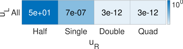
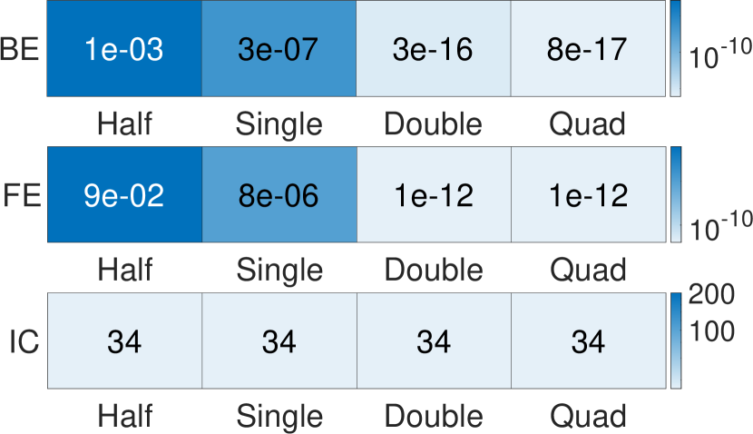
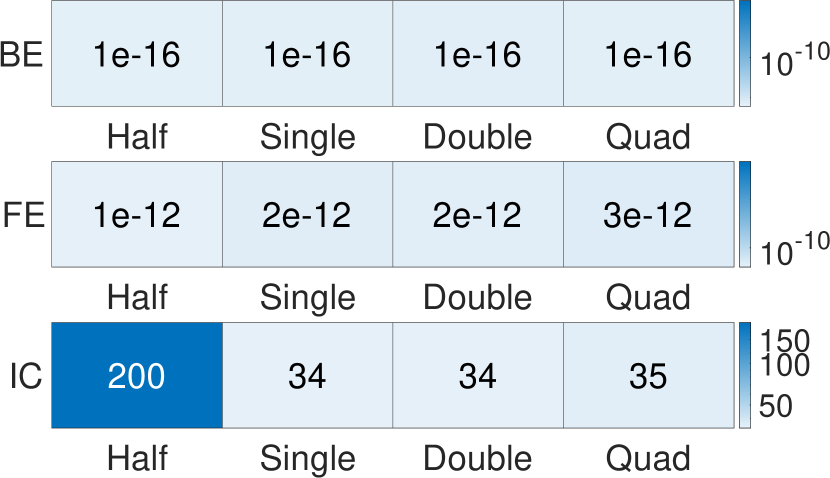
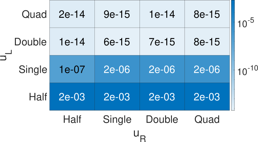
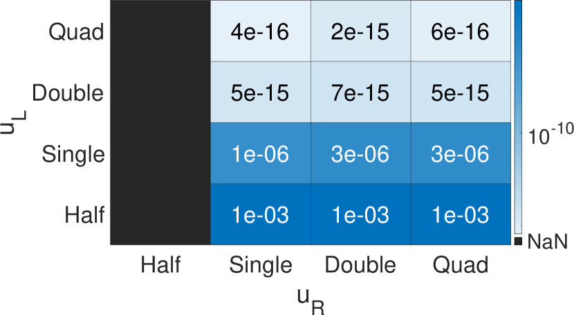
We set the working precision to double. Bounds for in Table 2 indicate that there is no need for , thus we choose . The preconditioners are applied using all combinations of half, single, double, and quadruple precisions. Half precision is simulated via the chop function [11], and Advanpix is used for quadruple precision. We expect to be a large overestimate for . suggests that the condition in (8) should be satisfied with set to any of the four precisions, except half for large values. We approximate by in Table 2, where we round to the nearest whole number. If is set to half precision, then , which is slightly smaller than the values of for . This indicates that applying in half precision may affect the backward error, however note that our choice for is expected to be an overestimate. The solver tolerance (see Algorithm 1) is set to and we use . For the unpreconditioned system, FGMRES converges in 200 iterations when and does not converge for other values.
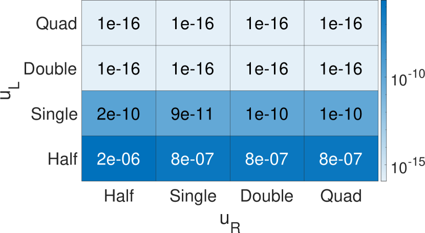
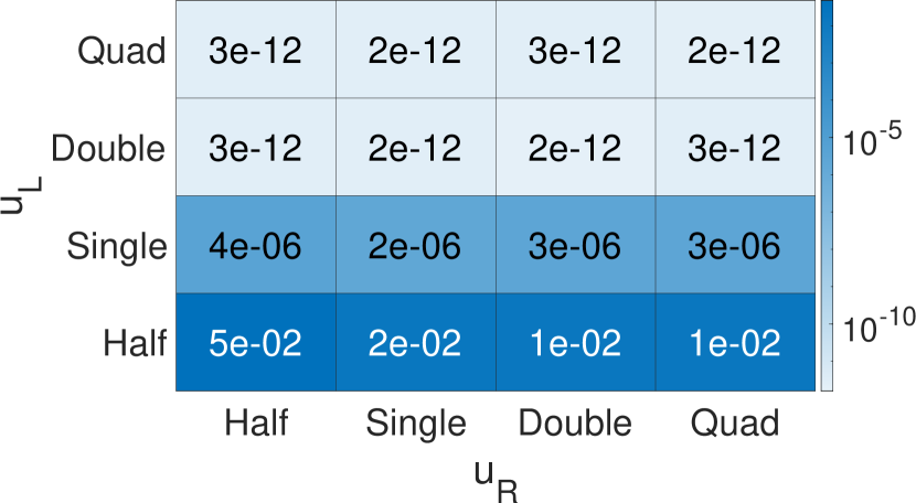
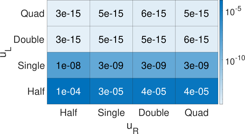
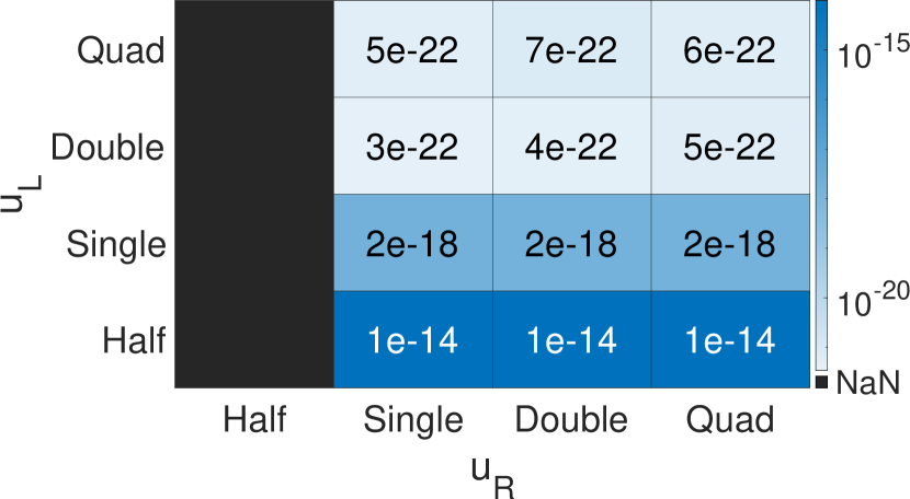
We show results for for all precision combinations (Figure 1), and for all values with set to single and set to double (Table 3), and set to double and set to single (Table 4). We report the relative backward error (BE) of the original problem, that is,
and compute the dominant part of the backward error bound (as defined in (12)). Note that bounds the relative backward error for the left-preconditioned system.
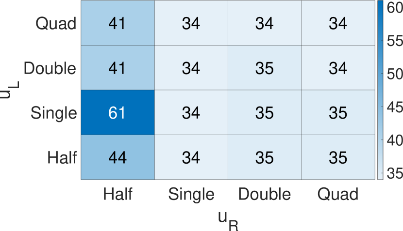
From Figure 1, we can see that the achievable backward error and subsequently the forward error depends on . As expected from theory, does not affect the achievable backward error, however influences the iteration count. Setting to half results in extra iterations when , and (not shown). Note that setting to quadruple, and to double or quadruple does not give any benefit. As mentioned, the backward error bound (11) is dominated by . From Tables 3 and 4, we can see that the quantity can become large, but it stays of the order of or close to it (not shown) and thus gives a good estimate of the backward error. If, however, is small, then the term can impair the bound. The increase in the forward error compared to the backward error is well estimated by , whereas is an overestimate. From Figure 1, we see that the condition is sufficient, but not necessary as it is not satisfied when and is set to half.
| c | bound | ||||||
| approx. | |||||||
| 1 | 10 | 1.06 | 615 | ||||
| 2 | 1.15 | 1551 | |||||
| 3 | 1.66 | 1853 | |||||
| 4 | 1949 | ||||||
| 5 | 2048 | ||||||
| 6 | 2144 | ||||||
| 7 | 2336 | ||||||
| 8 | 2551 | ||||||
| 9 | 2716 | ||||||
| 10 | 2768 |
| c | IC | BE | FE | |||||
|---|---|---|---|---|---|---|---|---|
| 1 | 6 | 1.21 | 2.22 | |||||
| 2 | 7 | 2.08 | ||||||
| 3 | 9 | 3.79 | ||||||
| 4 | 15 | 3.55 | ||||||
| 5 | 35 | 4.58 | ||||||
| 6 | 7 | 4.81 | ||||||
| 7 | 11 | 8.09 | ||||||
| 8 | 21 | 6.08 | ||||||
| 9 | 92 | 6.82 | ||||||
| 10 | 200 | 8.28 |
| c | IC | BE | FE | |||||
|---|---|---|---|---|---|---|---|---|
| 1 | 6 | 1.26 | 2.48 | |||||
| 2 | 7 | 1.66 | ||||||
| 3 | 9 | 3.46 | ||||||
| 4 | 15 | 3.19 | ||||||
| 5 | 34 | 3.86 | ||||||
| 6 | 7 | 4.28 | ||||||
| 7 | 11 | 6.23 | ||||||
| 8 | 21 | 5.18 | ||||||
| 9 | 158 | 8.79 | ||||||
| 10 | 200 | 7.62 |
3.2 Numerical example: left- and right-preconditioning
We also perform experiments with full left- (i.e., and ) and full right-preconditioning (i.e., and ) using the same set-up as in the previous section. For the left-preconditioning case using (18) we set and . Equivalently, for the right-preconditioning case and . Both left- and right-preconditioners are effective in reducing the condition number of the coefficient matrix (see Table 5). Note that the bounds for and in the left-preconditioning case indicate that may have to be applied in precision such that for all problems and we may need for highly ill-conditioned cases. For right-preconditioning, from (19) we know that can be bounded by and thus we can set . We use to approximate in Table 5. As in the split-preconditioning case, the values are larger than for half precision.
Experiments with set to double (Table 6) show that the bounds for in Table 5 largely overestimate the error in applying the preconditioner and even though the bounds for are quite close to the obtained values, we still obtain relative backward error for the unpreconditioned system. Note that the values are increased by . If we keep set to double and set to single, the relative backward error for the unpreconditioned system reaches and determines (Table 3). This agrees with the split-reconditioning results.
We keep set to double for right-preconditioning experiments (Tables 8 and 9). Note that the relative backward error reaches with set to both double and single, except for with set to single. The number of iterations when is set to single grows for highly ill-conditioned problems. Though the term grows as in the split-preconditioning case, it is balanced by here. Note that in these experiments the bound in [4, eq. (3.22) ] is applicable for . Here and the term is thus small ensuring a tight bound for the backward error.
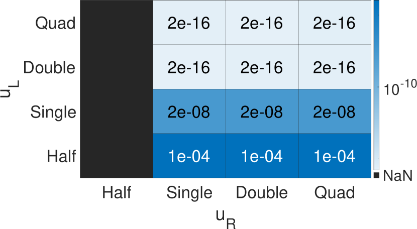
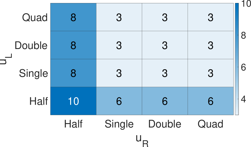
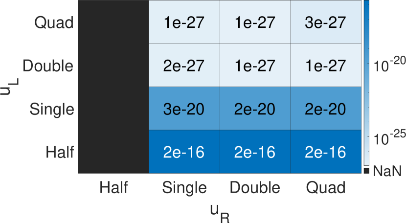
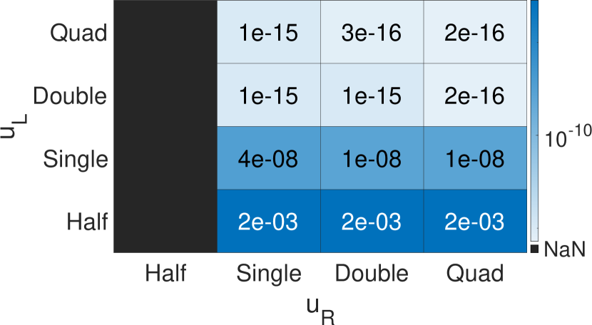
The results for for all choices of and are presented in Figure 2. Comparing these with the skew diagonals (/) of the respective heatmaps in Figure 1, that is, when the preconditioners are applied in the same precision, shows that applying the full preconditioner on the left gives larger relative backward and consequentially forward errors when the preconditioner is applied in low precision. This is not the case when the full preconditioner is applied on the right. It is curious that the iteration count with left-, right- and split-preconditioning is essentially different only when the preconditioner is applied in half precision. The results for different values are similar.
| left-preconditioning | right-preconditioning | ||||
| c | bound | bound | approx. | ||
| 1 | |||||
| 2 | |||||
| 3 | |||||
| 4 | |||||
| 5 | |||||
| 6 | |||||
| 7 | |||||
| 8 | 7.56 | ||||
| 9 | |||||
| 10 | |||||
| c | IC | BE | FE | |||
|---|---|---|---|---|---|---|
| 1 | 6 | 6.41 | ||||
| 2 | 7 | |||||
| 3 | 9 | |||||
| 4 | 15 | |||||
| 5 | 34 | |||||
| 6 | 7 | |||||
| 7 | 11 | |||||
| 8 | 21 | |||||
| 9 | 47 | |||||
| 10 | 124 |
| c | IC | BE | FE | |||
|---|---|---|---|---|---|---|
| 1 | 6 | 6.48 | ||||
| 2 | 7 | |||||
| 3 | 9 | |||||
| 4 | 15 | |||||
| 5 | 34 | |||||
| 6 | 7 | |||||
| 7 | 11 | |||||
| 8 | 21 | |||||
| 9 | 47 | |||||
| 10 | 114 |
| c | IC | BE | FE | ||||
|---|---|---|---|---|---|---|---|
| 1 | 6 | 1.41 | |||||
| 2 | 7 | ||||||
| 3 | 9 | ||||||
| 4 | 15 | ||||||
| 5 | 34 | ||||||
| 6 | 7 | ||||||
| 7 | 11 | ||||||
| 8 | 21 | ||||||
| 9 | 61 | ||||||
| 10 | 200 |
| c | IC | BE | FE | ||||
|---|---|---|---|---|---|---|---|
| 1 | 6 | ||||||
| 2 | 7 | ||||||
| 3 | 9 | ||||||
| 4 | 15 | ||||||
| 5 | 34 | ||||||
| 6 | 7 | ||||||
| 7 | 11 | ||||||
| 8 | 27 | ||||||
| 9 | 200 | ||||||
| 10 | 200 |
3.3 Numerical example: application problems with split-preconditioning
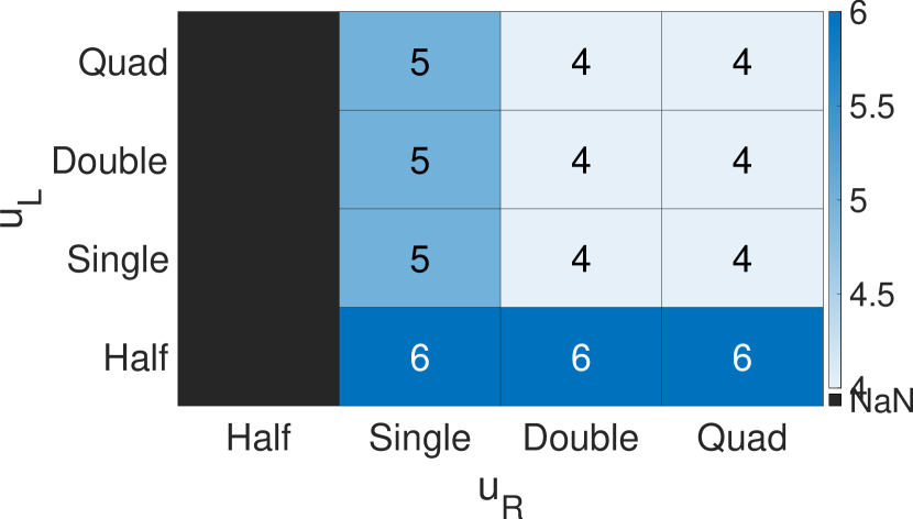
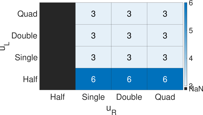
We perform experiments with some ill-conditioned problems from the SuiteSparse collection [8]; see Table 10. We generate the right hand side vector in the same way as for the synthetic problems. The preconditioner is computed as in the previous section, but in single precision, and the matrix is converted to a full matrix due to the lacking single precision sparse matrix-vector product functionality in MATLAB. We report results for split-preconditioning only; these illustrate the trends in left- and right-preconditioning cases well. Note that the split-preconditioner reduces the condition number to the theoretical minimum or close to it, except for the problem with the highest . However and are of the order of and thus we expect to see its effect on the forward error. We set and to double based on the bound; and are set as in the previous sections. Unpreconditioned FGMRES does not converge in iterations for any of the problems.
Approximations of indicate that the backward error may be affected if we apply in half precision for arc130 and west0132. However, we cannot test this as for all problems except rajat14, is singular with respect to set to half. This may be amended by using scaling strategies when computing the preconditioner; see, for example, [12]. We observe similar tendencies (Figures 3 and 4) as for the dense problems, however here we can achieve smaller backward error and for fs_183_3 the backward error is even with set to half. Note that for sparse problems setting to a low precision results in iteration-wise slower convergence. The term grows as for the dense problems, but is balanced by ; see Tables 11 and 12.
In all of our sparse and dense examples, does not become large enough to allow setting without it affecting the backward error. However for fs_183_3 both and are small enough that we can set and to single and expect backward error. Numerical experiments confirm this even though the backward and forward errors become slightly larger compared to set to double (not shown).
| problem | bound | |||||||
| approx. | ||||||||
| rajat14 | 180 | 1.01 | 1.13 | 33 | ||||
| arc130 | 130 | 1.00 | 2.64 | 1.00 | 479471 | |||
| west0132 | 132 | 1.12 | 7.49 | 1.00 | 3619199 | |||
| fs_183_3 | 183 | 1.00 | 267 |
| problem | IC | BE | FE | |||||
|---|---|---|---|---|---|---|---|---|
| rajat14 | 3 | |||||||
| arc130 | 3 | |||||||
| west0132 | 4 | |||||||
| fs_183_3 | 3 |
| problem | IC | BE | FE | |||||
|---|---|---|---|---|---|---|---|---|
| rajat14 | 3 | |||||||
| arc130 | 5 | |||||||
| west0132 | 5 | |||||||
| fs_183_3 | 3 |


4 Concluding remarks
In light of great community focus on mixed precision computations, we analyzed a variant of split-preconditioned FGMRES that allows using different precisions for computing matrix-vector products with the coefficient matrix (unit roundoff ), left-preconditioner (unit roundoff ), right-preconditioner (unit roundoff ), and other computations (unit roundoff ). A backward error of a required level can be achieved by controlling these precisions.
Our analysis and numerical experiments show that the precision for applying must be chosen in relation to , , and the required backward and forward errors, because heavily influences the achievable backward error. We can be more flexible when choosing as it does not influence the backward error directly. Our analysis holds under a sufficient but not necessary assumption on in relation to . As long as is not singular in precision (note that scaling strategies may be used to ensure this), setting to a low precision is sufficient. Very low precisions and may delay the convergence iteration wise, yet setting or does not improve the convergence in general. Note that these conclusions apply to the full left- and right-preconditioning cases as well.
We observe that the forward error is determined by the backward error and the condition number of the left-preconditioned coefficient matrix. This motivates concentrating effort on constructing an appropriate left-preconditioner when aiming for a small forward error: the preconditioner should reduce the condition number sufficiently and needs to be applied in a suitably chosen precision.
Appendix A Proof of Theorem 2.1
The analysis closely follows [5] and [4], and thus we provide the important results for each stage rather than the step-by-step analysis.
A.1 Left preconditioner
We start by accounting for the effect of .
A.1.1 Stage 1: MGS
In this stage, we use precisions , and . MGS is applied to
MGS returns an upper triangular and there exists an orthonormal , that is , such that
| (20) | |||
| (21) | |||
| (22) | |||
| (23) | |||
| (24) |
Here is the error in computing the matrix vector product and accounts for computing and adding it to the computed . Error comes from computing . and arise in the MGS process.
A.1.2 Stage 2: Least squares
The least squares problem is solved using precision .
A.1.3 Stage 3: Computing
When certain conditions on the residual norm are satisfied, precision is used to compute as
| (30) | |||
| (31) |
Using this to eliminate in (25), then applying the reverse triangle inequality to bound and bounding , and gives
| (32) |
We eliminate from the bound in the following section.
A.2 Right preconditioner
References
- [1] A. Abdelfattah, H. Anzt, E. G. Boman, E. Carson, T. Cojean, J. Dongarra, A. Fox, M. Gates, N. J. Higham, X. S. Li, et al., A survey of numerical linear algebra methods utilizing mixed-precision arithmetic, The International Journal of High Performance Computing Applications, 35 (2021), pp. 344–369.
- [2] Advanpix multiprecision computing toolbox for MATLAB. http://www.advanpix.com.
- [3] P. Amestoy, A. Buttari, N. J. Higham, J.-Y. L’Excellent, T. Mary, and B. Vieublé, Five-precision gmres-based iterative refinement, MIMS EPrint 2021.5, Manchester Institute for Mathematical Sciences, The University of Manchester, Manchester, UK, Apr. 2021.
- [4] M. Arioli and I. S. Duff, Using FGMRES to obtain backward stability in mixed precision, Electronic Transactions on Numerical Analysis, 33 (2009), pp. 31–44. https://etna.math.kent.edu/vol.33.2008-2009/pp31-44.dir/.
- [5] M. Arioli, I. S. Duff, S. Gratton, and S. Pralet, A note on GMRES preconditioned by a perturbed decomposition with static pivoting, SIAM Journal on Scientific Computing, 29 (2007), pp. 2024–2044.
- [6] E. Carson and N. J. Higham, A new analysis of iterative refinement and its application to accurate solution of ill-conditioned sparse linear systems, SIAM Journal on Scientific Computing, 39 (2017), pp. A2834–A2856.
- [7] E. Carson, N. J. Higham, and S. Pranesh, Three-precision GMRES-based iterative refinement for least squares problems, SIAM Journal on Scientific Computing, 42 (2020), pp. A4063–A4083.
- [8] T. A. Davis and Y. Hu, The University of Florida sparse matrix collection, ACM Trans. Math. Softw., 38 (2011).
- [9] N. J. Higham, Accuracy and Stability of Numerical Algorithms, Society for Industrial and Applied Mathematics, Philadelphia, PA, USA, second ed., 2002.
- [10] N. J. Higham and T. Mary, Mixed precision algorithms in numerical linear algebra, Acta Numerica, 31 (2022), p. 347–414.
- [11] N. J. Higham and S. Pranesh, Simulating low precision floating-point arithmetic, SIAM J. Sci. Comput., 41 (2019), pp. C585 – C602.
- [12] N. J. Higham, S. Pranesh, and M. Zounon, Squeezing a matrix into half precision, with an application to solving linear systems, SIAM Journal on Scientific Computing, 41 (2019), pp. A2536 – A2551.
- [13] N. Lindquist, P. Luszczek, and J. Dongarra, Improving the performance of the GMRES method using mixed-precision techniques, in Driving Scientific and Engineering Discoveries Through the Convergence of HPC, Big Data and AI: 17th Smoky Mountains Computational Sciences and Engineering Conference, SMC 2020, Oak Ridge, TN, USA, August 26-28, 2020, Revised Selected Papers 17, Springer, 2020, pp. 51–66.
- [14] NVIDIA H100 Tensor Core GPU. NVIDIA, https://www.nvidia.com/en-us/data-center/h100/, 2023.
- [15] C. C. Paige, M. Rozložník, and Z. Strakoš, Modified Gram-Schmidt (MGS), least squares, and backward stability of MGS-GMRES, SIAM Journal on Matrix Analysis and Applications, 28 (2006), pp. 264–284.
- [16] Y. Saad, Iterative methods for sparse linear systems, Society for Industrial and Applied Mathematics, Philadelphia, PA, USA, 2003.
- [17] B. Vieublé, Mixed precision iterative refinement for the solution of large sparse linear systems, PhD thesis, INP Toulouse, University of Toulouse, France, 2022.