Quantifying the Safety of Trajectories
using Peak-Minimizing Control

Abstract

This work quantifies the safety of trajectories of a dynamical system by the perturbation intensity required to render a system unsafe (crash into the unsafe set). Computation of this measure of safety is posed as a peak-minimizing optimal control problem. Convergent lower bounds on the minimal peak value of controller effort are computed using polynomial optimization and the moment-Sum-of-Squares hierarchy. The crash-safety framework is extended towards data-driven safety analysis by measuring safety as the maximum amount of data corruption required to crash into the unsafe set.

1 Introduction

A trajectory starting at an initial point $x_{0}\in X$ following dynamics $\dot{x}=f_{0}(t,x)$ is safe with respect to the unsafe set $X_{u}$ in the time horizon $t\in[0,T]\subset[0,\infty)$ if there does not exist a time $t^{\prime}$ such that $x(t^{\prime}\mid x_{0})$ is a member of $X_{u}$. The set $X_{0}$ is safe with respect to $X_{u}$ if all initial points $x_{0}\in X_{0}$ generate safe trajectories. This paper quantifies the safety of trajectories by maximum control effort ( Optimal Control Problem (OCP) cost) needed to crash the agent into the unsafe set. An example of this type of safety result is if tilting a car’s steering wheel by a maximum extent of $3^{\circ}$ over the course of its motion would cause the car to crash. The process of analyzing safety by peak-minimizing-OCP cost will be referred to as ‘crash safety’. This crash-safety will also be used in the data-driven framework, in which a trajectory is labeled safe if it would require the true system to have a large constraint violation against any of its state-derivative data observations in order to crash.

Let $W\subset\mathbb{R}^{L}$ be a compact input set, and let $\mathcal{W}$ be the class of functions whose graphs satisfy $(t,w(t))\in[0,T]\times W$. Given a control-cost $J(w)$, we can pose the following peak-minimizing free-terminal-time OCP:

$$Q^{*}= \inf_{t,\ x_{0},\ w}\ \sup_{t^{\prime}\in[0,t]}J(w(t^{\prime}))$$ (1)

$$\dot{x}(t^{\prime})=f(t^{\prime},x(t^{\prime}),w(t^{\prime})) \forall t^{\prime}\in[0,T]$$

$$x(t\mid x_{0},w(\cdot))\in X_{u}$$

$$w(\cdot)\in\mathcal{W},\ t\in[0,T],\ x_{0}\in X_{0}.$$

The variables of (1) are the stopping time $t$, the initial condition $x_{0}$, and the input process $w(\cdot)$. Assuming for the purposes of this introduction that $J(0)=0,\ \forall w\neq 0:J(w)>0$ and that $J$ possesses connected superlevel sets, the set $x_{0}$ is unsafe if $Q^{*}=0$ because the process $w(t)=0$ is sufficient for the trajectory to reach a terminal set of $X_{u}$. The value of a nonzero $Q^{*}$ then measures the amount of control effort (perturbation intensity) needed to render the trajectory unsafe. Connected level sets are imposed to add interpretability to $Q^{*}$; a disconnected choice of $J$ with multiple local minima could yield a large input $w$ with a low $Q^{*}$.

A running cost $\int_{0}^{T}J(w(t^{\prime}))dt$ yielding a standard-form (Lagrange) OCP may also be applied, but we elect to use a peak-minimizing cost $\max_{t^{\prime}}J(w(t^{\prime}))$ in order to penalize perturbation intensity. The running-cost would penalize a low-magnitude control being applied for an extended period of time, while peak-minimizing control reduces the intensity.

Peak-minimizing control problems, such as in (1), are a particular form of robust optimal control in which the minimizing agents are $(t,x_{0},w(\cdot))$ and the maximizing agent is $t^{\prime}\in[0,t]$. Necessary conditions for these robust programs may be found in [1]. Instances of peak-minimizing control include minimizing the maximum number of infected persons in an epidemic under budget constraints [2] and choosing flight parameters to minimize the maximum skin temperature during atmospheric reentry [3, 4]. The work in [5] outlines conversions between peak-minimizing OCPs and equivalent Mayer-form OCPs (terminal cost only).

This paper continues a sequence of research about quantifying the safety of trajectories. Unsafety can be proven using path-planning by finding a feasible pair $(t^{\prime},x_{0})\in[0,T]\times X_{0}$ such that $x(t^{\prime}\mid x_{0})\in X_{0}$. Barrier [6, 7] and Density functions [8] are binary certificates confirming that there does not exist an unsafe trajectory based on the satisfaction of nonnegativity constraints. Safety margins use maximin peak estimation to estimate the $X_{u}$-representing-inequality-constraint violation [9]. The distance of closest approach between a trajectory starting in $X_{0}$ and points in $X_{u}$ is a more interpretable measure of safety than abstract safety margins [10]. Even so, distance estimation does not tell the full story; a trajectory may lie close to $X_{u}$ in the sense of distance, but it could require a large value of $Q^{*}$ to render the same trajectory unsafe.

Direct solution of OCPs using the Hamilton-Jacobi-Bellman (HJB) equation or the Pontryagin Maximum Principle may be challenging, especially when solutions do not exist in closed form [11]. These generically non-convex OCPs may be lifted into convex infinite-dimensional Linear Programs in occupation measures [12], whose dual LP involve subvalue functions satisfying HJB inequalities. These infinite-dimensional LPs produce lower-bounds on the true OCP, with equality holding under compactness and regularity conditions. The moment- Sum of Squares (SOS) hierarchy of Semidefinite Programs may be used to produce a rising sequence of lower bounds to the true OCP if the dynamics $f(t,x,w)$ are polynomial and the sets $(W,X,X_{0},X_{u})$ are Basic Semialgebraic (BSA) [13]. This infinite-dimensional LP and finite-dimensional SDP pattern has also been applied to reachable set estimation [14, 15], peak estimation [16, 17], and maximum controlled invariant set estimation [18].

This paper transforms program (1) into the Mayer OCP using [5], relaxes the nonconvex OCP into an infinite-dimensional LP with the same objective value [12], and then lower-bounds $Q^{*}$ by using the moment-SOS hierarchy [13, 19]. The robust counterpart method of [20, 21] will be used to simplify the infinite-dimensional LP when $W$ and the graph of $J$ are both polytopic. Contributions of this work include,

• An interpretation of peak-minimal control costs as a quantification of safety

• An infinite-dimensional LP that produces the peak-minimal cost under compactness, regularity, and convexity conditions

• A subvalue functional that lower-bounds the crash-safety effort

• An application of crash-safety towards data-driven safety analysis

This paper has the following structure: Section 2 reviews the notations, the peak-minimizing control framework of [5], and SOS methods. Section 3 formulates an infinite-dimensional LP to solve (1). Section 4 applies the crash-safety framework towards $L_{\infty}$-penalized data-driven analysis using robust Lie counterparts from [21]. Section 5 forms SOS programs for crash-safety and tabulates their computational complexity. Section 6 evaluates the safety of points inside $X$ by a subvalue function of the crash-safety cost. Section 7 provides demonstrations of crash-safety. Section 8 concludes the paper.

2 Preliminaries

2.1 Acronyms/Initialisms

BSA

Basic Semialgebraic

LMI

Linear Matrix Inequality

HJB

Hamilton-Jacobi-Bellman

LP

Linear Program

OCP

Optimal Control Problem

PD

Positive Definite

PSD

Positive Semidefinite

SDP

Semidefinite Program

SDR

Semidefinite Representable

SOS

Sum of Squares

WSOS

Weighted Sum of Squares

2.2 Notation

The set of real numbers is $\mathbb{R}$ and the $n$-dimensional real vector spaces is $\mathbb{R}^{n}$. The all-ones vector is $\mathbf{1}$. The set of natural numbers is $\mathbb{N}$ and the set of $n$-dimensional multi-indices is $\mathbb{N}^{n}$. The set of natural numbers between $a$ and $b$ is $a..b\subset\mathbb{N}$. The cone of $n\times n$ symmetric Positive Semidefinite (PSD) matrices is $\mathbb{S}^{n}_{+}$.

The set of polynomials of an indeterminate $x$ with real-valued coefficients is $\mathbb{R}[x]$. The degree of a polynomial $p\in\mathbb{R}[x]$ is $\deg p$. The vector space of polynomials up to degree $d\in\mathbb{N}$ is $\mathbb{R}[x]_{\leq d}$. The coefficients of a polynomial $p\in\mathbb{R}[x]$ are $\text{coeff}_{x}(p(x))$.

The ring of continuous functions over a space $S\subseteq\mathbb{R}^{n}$ is $C(S)$. The set of first-differentiable functions over $S$ is $C^{1}(S)\subset C(S)$. The subcone of nonnegative functions over $S$ is $C_{+}(S)\subset C(S)$.

The set of nonnegative Borel measures over $S$ is $\mathcal{M}_{+}(S)$. Given a measure $\mu\in\mathcal{M}_{+}(S)$, the support $\textrm{supp}(\mu)$ is the locus of points $s^{\prime}\in S$ such that every open neighborhood of $s^{\prime}$ has a nonzero measure with respect to $\mu$. A pairing $\langle\cdot,\cdot\rangle$ may be defined between $f\in C(S)$ and $\mu\in\mathcal{M}_{+}(S)$ by $\langle f,\mu\rangle=\int_{S}f(s)d\mu(s)$. This pairing defines an inner product between $C_{+}(S)$ and $\mathcal{M}_{+}(S)$ when the set $S$ is compact. The mass of a measure $\mu\in\mathcal{M}_{+}(S)$ is $\langle 1,\mu\rangle,$ and $\mu$ is a probability measure if $\langle 1,\mu\rangle=1$. The Dirac delta $\delta_{s^{\prime}}$ is the unique probability supported only at $s^{\prime}\in S$, with $\forall f\in C(S):\langle f,\delta_{s^{\prime}}\rangle=s^{\prime}$. Given a curve $s:[0,T]\times S$, the occupation measure $\mu_{s}$ of $s(t)$ in the times $[0,T]$ is the unique measure satisfying $\forall v\in C([0,T]\times S):\langle v(t,s),\mu_{s}\rangle=\int_{0}^{T}v(t,s(t))dt$.

2.3 Peak Minimizing Control

This section reviews the peak-minimizing control problem and a simplified conversion framework based on [5]. Given an objective $\theta:[0,T]\times X\times W\rightarrow\mathbb{R}$, an initial condition $x_{0}$, and a fixed terminal time $T$, the peak-minimizing control problem is

$$P^{*}= \inf_{w\in\mathcal{W}}\quad\sup_{t^{\prime}\in[0,T]}\theta(t^{\prime},x(t^{\prime}\mid x_{0},w(\cdot)),w(t^{\prime})))$$ (2)

$$\dot{x}(t)=f(t^{\prime},x(t^{\prime}),w(t^{\prime}))\qquad\forall t\in[0,T].$$

The work in [5] details three different methods to convert a peak-minimizing control OCP into a Mayer OCP: pure state constraint, mixed state constraint, and differential inclusion. We will elect to use the first method in [5], which involves the augmentation of constant dynamics by a new state $\dot{z}=0$:

$$P^{*}_{z}= \inf_{w\in\mathcal{W},z\in\mathbb{R}}\quad z$$ (3)

$$\dot{x}(t)=f(t,x(t),w(t)) \forall t\in[0,T]$$

$$\dot{z}=0 \forall t\in[0,T]$$

$$z\geq\theta(t^{\prime},x(t^{\prime}\mid x_{0},w(\cdot)),w(t^{\prime})) \forall t^{\prime}\in[0,T].$$

The parameter $z$ always remains an upper bound on $p$ along trajectories, and the controller $w(\cdot)$ is chosen to reduce this upper bound as much as possible.

Proposition 2.1 (Proposition 3.1 of [5]).

The objectives $P^{*}$ and $P^{*}_{z}$ are equal between (3) and (2).

2.4 Sum of Squares

Verifying that a polynomial $p\in\mathbb{R}[x]$ is nonnegative $\forall x\in\mathbb{R}^{n}$ is generically an NP-hard problem (except for $p$ quadratic, univariate, or bivariate quartic) [22]. A sufficient condition for $p$ to be nonnegative is if there exists $N$ factors $\{p_{k}\in\mathbb{R}[x]\}_{k=1}^{N}$ such that $p=\sum_{k=1}^{N}p_{k}(x)^{2}$. Such a $p$ is therefore called an SOS polynomial. The cone of SOS polynomials is $\Sigma[x]$, and the subset of degree $\leq 2d$ SOS polynomials is $\Sigma[x]_{d}\subset\Sigma[x]$. To each polynomial $p\in\Sigma[x]_{d}$, there exists an $s$-dimensional vector of polynomials $v(x)$ (e.g. monomials up to degree $d$) and PSD PSD Gram matrix $Q\in\mathbb{S}_{+}^{s}$ such that $p(x)=v(x)^{T}Qv(x)$. When the monomial basis is used, the Gram matrix has dimension $\binom{n+d}{d}$. Verification of $p\in\Sigma[x]_{2d}$ at fixed degree can be performed by solving SDP SDP. The per-iteration scaling of Interior Point Methods for solving this SDP rises in a jointly polynomial manner with $n$ and $d$ (with $O(n^{6d})$ and $O(d^{4n})$) [23] [24].

BSA BSA set $\mathbb{K}\in\mathbb{R}^{n}$ is a set formed by the locus of a finite number of inequality and equality constraints of bounded degree:

$$\mathbb{K} =\{x\mid\forall i=1..N_{g}:\ g_{i}(x)\geq 0,\ \forall i=1..N_{h}:\ h_{j}(x)=0\}.$$ (4)

A sufficient condition for $p\in\mathbb{R}[x]$ to be nonnegative over $\mathbb{K}$ is that there exists multipliers $\sigma_{0},\sigma_{i},\phi_{j}$ such that [25]

$$p(x)=\sigma_{0}(x)+\textstyle\sum_{i}{\sigma_{i}(x)g_{i}(x)}+\textstyle\sum_{j}{\theta_{j}(x)h_{j}(x)}$$ (5a)

$$\exists\sigma_{0}(x)\in\Sigma[x],\quad\sigma_{i}(x)\in\Sigma[x],\quad\phi_{j}\in\mathbb{R}[x].$$ (5b)

The Weighted Sum of Squares (WSOS) cone $\Sigma[\mathbb{K}]$ is the set of polynomials that admit a representation as in (5). The truncated WSOS set $\Sigma[\mathbb{K}]_{d}$ is the set of polynomials where the certificate in (5) has $\deg\sigma_{0}\leq 2d,\ \forall i:\deg\sigma_{i}g_{i}\leq 2d,$ and $\forall j:\deg\phi_{j}h_{j}\leq 2d$. Verification of $p\in\Sigma[\mathbb{K}]$ could require multipliers that have an exponential degree in $n$ and $\deg p$ [26].

The BSA set $\mathbb{K}$ is Archimedean if there exists $R\in[0,\infty)$ such that $R-\lVert x\rVert_{2}^{2}\in\Sigma[\mathbb{K}]$. Archimedeanness is a stronger property than compactness [27]. If there exists a known $\tilde{R}$ verifying compactness such that $\mathbb{K}\subseteq\{x\in\mathbb{R}^{n}\mid\lVert x\rVert_{2}^{2}\leq\tilde{R}\},$ then the compact set $\mathbb{K}$ may be rendered Archimedean by adding the redundant ball constraint $\tilde{R}-\lVert x\rVert^{2}_{2}\geq 0$ to the list of constraints in (4). When $\mathbb{K}$ is Archimedean, the Putinar Positivestellensatz states that every positive polynomial over $\mathbb{K}$ is a member of $\Sigma[\mathbb{K}]$ [25, Theorem 1.3]. The moment-SOS hierarchy is the process of increasing the degree $d$ in $\Sigma[\mathbb{K}]_{d}$ to eventually include the set of all positive polynomials.

3 Crash-Safety Program

This section applies peak-minimizing control conversion to the crash-safety task in (1).

3.1 Motivating Example

This subsection provides an example demonstrating how (1) can be used for safety quantification. The Flow dynamics from [8] are

$$\dot{x}=\begin{bmatrix}x_{2}\\ -x_{1}-x_{2}+\frac{1}{3}x^{3}_{1}\end{bmatrix}.$$ (6)

This example will perturbed (6) by an uncertainty process restricted to $\forall t:\ w(t)\in[-1,1]$:

$$\dot{x}=\begin{bmatrix}x_{2}\\ -x_{1}-x_{2}+\frac{1}{3}x^{3}_{1}\end{bmatrix}+w\begin{bmatrix}0\\ 1\end{bmatrix}.$$ (7)

Trajectories evolve over a time horizon of $T=5$ in the state set $X=[-0.6,1.75]\times[-1.5,1.5]$ with a maximum corruption of $J_{\max}=2$. System dynamics are illustrated by the blue streamlines in Figure 1. The red half-circle is the unsafe set $X_{u}=\{x\mid x_{2}\leq-0.5,\ (x_{1}-1)^{2}+(x_{2}+0.5)^{2}\leq 0.5^{2}\}$. Two trajectories of this system are highlighted. The green trajectory starts from the top initial point $X^{1}_{0}=[0;1],$ and the yellow trajectory starts from the bottom initial point $X^{2}_{0}=[1.2966-1.5]$. The distance of closest approach to $X_{u}$ is $0.2498$ for both trajectories (matching up to four decimal places). The $0.2498$-contour of constant distance is displayed by the red curve surrounding $X_{u}$.

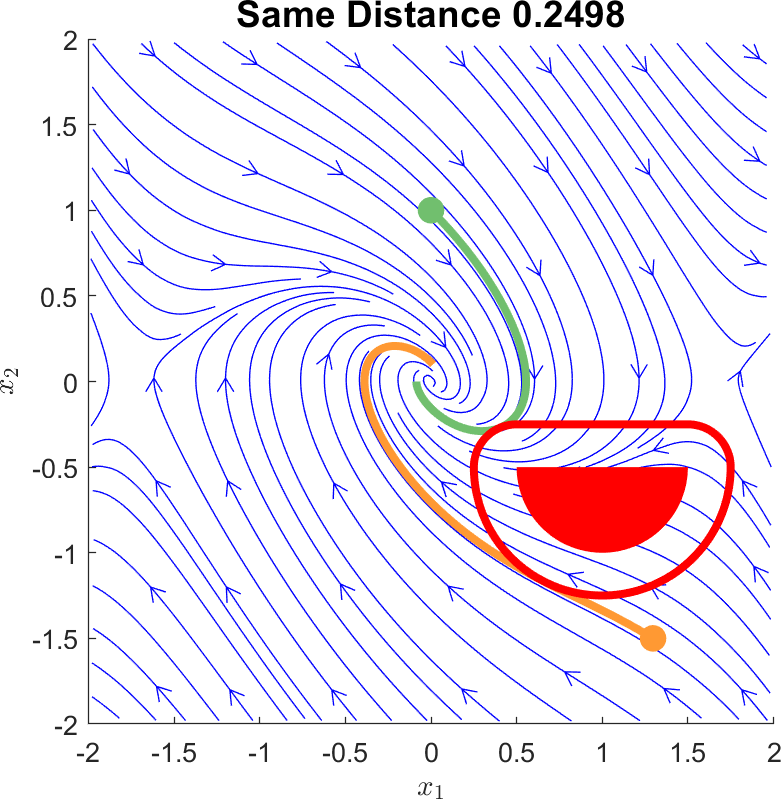
Figure 1: Two trajectories with nearly the same distance but different crash-bounds

The OCP solver CasADi [28] returns approximate bounds for (1) of $Q^{*}\approx 0.3160$ for $X_{0}^{1}$ (green) and $Q^{*}\approx 0.6223$ for $X_{0}^{2}$ (yellow). The points $(X^{1}_{0},X^{2}_{0})$ return nearly identical distances of closest approach, but $X^{2}_{0}$ may be judged as safer than $X^{1}_{0}$ under the disturbance model in (6) due to its higher crash-bound value. Degree-4 SOS tightenings of (8) developed in the sequel return lower bounds of $0.3018$ and $0.5273$ respectively.

3.2 Assumptions

We will require the following assumptions:

1. The sets $[0,T],[0,J_{\max}],X,W,X_{u},X_{0}$ are all compact.

2. The image $f(t,x,W)$ is convex for each fixed $(t,x)$.

3. The dynamics function $f(t,x,w)$ is Lipschitz in the compact domain $[0,T]\times X\times W$.

4. If $x(t\mid x_{0},w)\,\in\partial X$ for some $t\in[0,T],\ x_{0}\in X_{0},\ w\in\mathcal{W}$, then $x(t^{\prime}\mid x_{0})\not\in X\ \forall t^{\prime}\in(t,T]$.

A4 is an assumption of non-return used in [10] that is weaker than ensuring $X$ is an invariant set.

3.3 Formulation

We use the peak-minimizing control conversion of [5] on program (1).

Theorem 3.1.

The following program has the same optimal value as (1):

$$Q^{*}_{z}= \inf_{t,\ x_{0},\ z,\ w}\ z$$ (8a)

$$\dot{x}(t^{\prime})=f(t^{\prime},x(t^{\prime}),w(t^{\prime})) \forall t^{\prime}\in[0,T]$$ (8b)

$$\dot{z}(t^{\prime})=0 \forall t^{\prime}\in[0,T]$$ (8c)

$$J(w(t^{\prime}))\leq z \forall t^{\prime}\in[0,T]$$ (8d)

$$x(t\mid x_{0},w(\cdot))\in X_{u}$$ (8e)

$$w(\cdot)\in W,\ t\in[0,T]$$ (8f)

$$x_{0}\in X_{0},z\in[0,J_{\max}].$$ (8g)

Proof.

This follows from Proposition 2.1 under the peak-function $\theta(t,x,w)=J(w).$ The following changes are made with respect to (3):

1. Free terminal time $t\in[0,T]$ with a terminal state constraint in $X_{u}$.

2. Free initial condition $x_{0}\in X_{0}$.

The state $z$ upper-bounds the worst-case control $\sup_{t^{\prime}\in[0,t]}J(w(t^{\prime}))$, yielding the peak-control-minimized cost $Q^{*}_{z}=Q^{*}$. ∎

3.4 Crash-Safety Linear Program

Define the following compact support sets involving the input $w$ and peak-bound $z$:

$$Z =[0,J_{\max}] \Omega =\{(w,z)\in W\times Z:J(w)\leq z\}.$$ (9)

Let $\mathcal{L}_{f}$ be the Lie derivative associated with $f$ for $v(t,x,z)\in C^{1}$ as

$$\mathcal{L}_{f}v(t,x,z,w)=(\partial_{t}+f(t,x,w)\cdot\nabla_{x})v(t,x,z).$$ (10)

An auxiliary function $v\in C^{1}$ may be defined to form an LP formulation of the crash-safety OCP in (1):

$$q^{*}= \sup_{\gamma\in\mathbb{R},\ v}\ \gamma$$ (11a)

$$\forall(x,z)\in X_{0}\times Z:$$

$$\qquad v(0,x,z)\geq\gamma\$$ (11b)

$$\forall(t,x,z)\in[0,T]\times X_{u}\times Z$$

$$\qquad v(t,x,z)\leq z\$$ (11c)

$$\forall(t,x,z,w)\in[0,T]\times X\times\Omega$$

$$\qquad\mathcal{L}_{f}v(t,x,z,w)\geq 0$$ (11d)

$$v(t,x,z)\in C^{1}([0,T]\times X\times Z).$$ (11e)

Theorem 3.2.

Under assumptions A1-A5, programs (1) and (11) will have equal objectives $q^{*}=Q^{*}$.

Proof.

Program (8) with optimum $Q^{*}_{z}$ is a standard-form OCP with free terminal time and zero running cost. Under assumptions A1-A5, Theorem 2.1 of [12] proves that $Q^{*}_{z}=q^{*}$. Section 6.3 of [12] specifically discusses state-dependent controls (e.g. $(w,z)\in\Omega$). Theorem 3.1 provides that $Q^{*}=Q^{*}_{z}$, which together implies that $Q^{*}=q^{*}$. ∎

The dual LP of (11) may be phrased in terms of an initial measure $\mu_{0}$, terminal measure $\mu_{u}$, and relaxed occupation measure $\mu$:

$$m^{*}= \ \inf_{\mu_{0},\mu_{p},\mu}\quad\langle z,\mu_{u}\rangle$$ (12a)

$$\langle v(t,x,z),\mu_{u}\rangle=\langle v(0,x,z),\mu_{0}\rangle+\langle\mathcal{L}_{f}v(t,x,z,w),\mu\rangle$$ (12b)

$$\langle 1,\mu_{0}\rangle=1$$ (12c)

$$\mu_{0}\in\mathcal{M}_{+}(X\times Z)$$ (12d)

$$\mu_{u}\in\mathcal{M}_{+}([0,T]\times X_{u}\times Z)$$ (12e)

$$\mu\in\mathcal{M}_{+}([0,T]\times X\times\Omega).$$ (12f)

Constraint (12a) is a Liouville equation involving the Young measure $\mu$ [29].

Lemma 3.3.

There exists a feasible solution to (12b)-(12f) under A1-A4.

Proof.

Let $t^{*}\in[0,T]$ be a stopping time, $x_{0}\in X_{0}$ be an initial condition, and $w(\cdot)\in\mathcal{W}$ be an input such that $x(t^{*}\mid x_{0},w(\cdot))\in X_{u}$. Let $z^{*}$ be a feasible solution to $\forall t\in[0,t^{*}]:(z^{*},w(t))\in\Omega$. Then the probability measures can be set to $\mu_{0}=\delta_{x=x_{0},z=z^{*}}$ and $\mu_{u}=\delta_{t=t^{*},x=x(t^{*}\mid x_{0},w(\cdot)),\ z=z^{*}}$, and $\mu$ can be assigned to the occupation measure of $t\mapsto(t,x(t^{*}\mid x_{0},w(\cdot)),w(t))$ in the times $[0,t^{*}]$. ∎

Remark 1.

The process of 3.3 to generate a feasible measure solution may be used when only A1 and A4 are active, thus certifying that $m^{*}\leq Q^{*}$.

Theorem 3.4.

Strong duality occurs with $q^{*}=d^{*}$ between (12) and (11) under assumptions A1-A4.

Proof.

This holds by standard OCP LP duality arguments from [12, 30], in which feasibility of a measure solution is demonstrated in Lemma 3.3. ∎

4 Data-Driven Crash-Safety Analysis

This section motivates crash-safety in the context of data-driven analysis. This section will remove the restriction that the performance function satisfies $J(0)=0$, but will retain the property that the level sets of $J$ are connected.

4.1 Data-Driven Overview

In this section, we will assume that $N_{s}$ time-state-derivative data records $\mathcal{D}=\{(t_{k},x_{k},y_{k})\}_{k=1}^{N_{s}}$ are provided for the true system $\dot{x}=F(t,x)$. The data records in $\mathcal{D}$ are corrupted by $L_{\infty}$-bounded noise of intensity $\epsilon$ with

$$\forall k=1..N_{s} \lVert y_{k}-F(t_{k},x_{k})\rVert_{\infty}\leq\epsilon.$$ (13)

We are given a dictionary of functions $(f_{0},\{f_{\ell}\}_{\ell=1}^{L})$ that are Lipschitz in $[0,T]\times X$ (e.g. monomials). We are also given the knowledge that there exists at least one ground-truth choice of parameters $w^{*}\in\mathbb{R}^{L}$ with

$$\textstyle F(t,x)=f_{0}(t,x)+\sum_{\ell=1}^{L}w^{*}_{\ell}f_{\ell}(t,x).$$ (14)

In the $L_{\infty}$-bounded polytopic framework, the crash-safety problem (8) finds an infimal upper bound on the data corruption needed to crash into the unsafe set:

$$Z^{*}= \inf_{t,\,x_{0},\,z,\,w}z$$ (15a)

$$\forall t^{\prime}\in[0,T]:$$

$$\qquad\dot{x}(t^{\prime})=f_{0}(t^{\prime},x)+\textstyle\sum_{\ell=1}^{L}w_{\ell}f_{\ell}(t^{\prime},x(t^{\prime}))$$ (15b)

$$\qquad\dot{z}(t^{\prime})=0$$ (15c)

$$x_{0}\in X_{0},\ x(t\mid x_{0},w)\in X_{u}$$ (15d)

$$\forall k=1..N_{s}:$$ (15e)

$$\qquad z\geq\lVert f_{0}(t_{k},x_{k})+\textstyle\sum_{\ell=1}^{L}w_{\ell}f_{\ell}(t_{k},x_{k})-y_{k}\rVert_{\infty}$$

$$z\in Z,\ w\in\mathbb{R}^{L},\ t\in[0,T].$$ (15f)

If the returned value of (15) is $Z^{*}=0$, then there exists some choice of model parameters $w$ that exactly fit the data $\mathcal{D}$ by (14). Additionally, this choice $w$ renders at least one trajectory $x(\cdot)$ starting from $X_{0}$ is unsafe (crashes into $X_{0}$). Values of $Z^{*}$ greater than 0 are a certificate of safety in the model structure. A larger value of $Z^{*}$ indicates that the data must be increasingly corrupted in order to render any trajectory unsafe. Safety is certified if $Z^{*}>\epsilon$, though we note that the true value of $\epsilon$ may be a-priori unknown.

4.2 Robust Data-Driven Program

We will use the input-affine structure of dynamics and polytopic form of (15) to form an LP that eliminates the uncertainty $w$. This elimination leads to increasingly tractable SOS SDPs. For each $k=1..N_{s}$, define the data-record matrices $\Gamma_{k},\ h_{k}$ by

$$\Gamma_{k} =\begin{bmatrix}f_{1}(t_{k},x_{k}),\cdots,f_{L}(t_{k},x_{k})\end{bmatrix}$$ (16a)

$$h_{k} =f_{0}(t_{k},x_{k})-y_{k}.$$ (16b)

Letting $\Gamma$ and $h$ be the vertical concatenations of $\{\Gamma_{k}\}$ and $\{h_{k}\}$ respectively, we can define the $L_{\infty}$ performance function and support set as

$$J(w) =\lVert\Gamma w-h\rVert_{\infty}=\theta(t,x,w),\quad Z=[0,J_{\max}],$$ (17)

and the support set for $$(w,z)$$ from (15) as

$$\Omega =\left\{(w,z)\in\mathbb{R}^{L}\times Z:\begin{matrix}\Gamma w\leq z\mathbf{1}-h\\ -\Gamma w\leq z\mathbf{1}+h\end{matrix}\right\}.$$ (18)

We will eliminate the $w$ variable from (11d) by introducing new nonnegative multiplier functions $\{\zeta^{+},\zeta^{-}_{j}\}_{j=1}^{2nT}$. This elimination proceeds using the infinite-dimensional robust counterpart method of [21], which requires that (11d) hold strictly (with a $>0$) constraint.

Theorem 4.1.

A strict version of Lie constraint in (11d) may be robustified (will have the same feasibility/infeasibility conditions) into

$$\forall(t,x,z)\in[0,T]\times X\times Z:$$

$$\qquad\mathcal{L}_{f_{0}}v-(z\mathbf{1}-h)^{T}\zeta^{+}-(z\mathbf{1}+h)^{T}\zeta^{-}>0$$ (19a)

$$\forall\ell=1..L:\quad\ (\Gamma^{T})_{\ell}(\zeta^{+}-\zeta^{-})+f_{\ell}\cdot\nabla_{x}v=0$$ (19b)

$$\forall j=1..2nT:\ \zeta^{+}_{j},\zeta^{-}_{j}\in C_{+}([0,T]\times X\times Z).$$ (19c)

Proof.

We define the following variables

$$b_{0} =\mathcal{L}_{f_{0}}v b_{\ell} =f_{\ell}\cdot\nabla_{x}v \forall\ell=1..L$$ (20a)

$$A =[-\Gamma;\Gamma] e =[z-h;z+h]$$ (20b)

$$K =\textstyle\prod_{s=1}^{2nT}\mathbb{R}_{\geq 0}.$$ (20c)

to express the strict version of (11d) into the form

$$\textstyle b_{0}+\sum_{\ell=1}^{L}w_{\ell}b_{\ell} >0 \forall Aw+e\in K.$$ (21)

The parameters of (21) are $(t,x,z)\in[0,T]\times X\times Z$. By Theorems 4.2 and 4.3 of [21], sufficient conditions for (19) to equal the strict version of (11d) are that:

• $K$ is a convex pointed cone.

• $[0,T]\times X\times Z$ is compact.

• $A$ is constant in $(t,x,z)$.

• $(e,b_{0},\{b_{\ell}\})$ are continuous in $(t,x,z)$.

R1 holds because $\mathbb{R}_{\geq 0}^{2nT}$ is a convex and pointed cone. Compactness of $[0,T]\times X$ holds by A1, and compactness of $Z$ holds by A2. R3 is true because $\Gamma$ is a constant matrix computed from the data in $\mathcal{D}$ from (16a). R4 is satisfied because $e$ is continuous (affine) in $z$, and $(b_{0},\{b_{\ell}\})$ are continuous given that $v\in C^{1}$ (11e) and $(f_{0},\{f_{\ell}\})$ are Lipschitz (A3). The theorem is proven because R1-R4 are all fullfilled. ∎

Remark 2.

Strictness in (19a) is required to ensure that $\zeta^{\pm}$ may be chosen to be continuous while not adding conservatism. A nonstrict inequality for (19a) may be developed using possibly discontinuous multipliers $\zeta^{\pm}$.

Remark 3.

This paper discussed $L_{\infty}$-bounded uncertainty, resulting in polytopic decomposition of the Lie constraint by Theorem 4.1. Theorems 4.2 and 4.4 of [21] may be applied when $\Omega$ is a more general semidefinite representable set parameterized by $z$, such as an intersection of ellipsoids for $L_{2}$-bounded noise, or a projection of spectahedra for semidefinite bounded noise.

5 SOS Programs

This section poses finite-dimensional SOS tightenings to the infinite-dimensional crash-safety programs.

We will require a strengthening of assumption A1:

• The sets $(X,X_{u},X_{0},[0,T],Z,\Omega)$ are all Archimedean BSA sets and the dynamics $f(t,x,w)$ are polynomial.

5.1 Standard Crash-Safety

For a given degree $d$, define $\tilde{d}=d+\lfloor\deg f/2\rfloor$ as the dynamics degree of $f(t,x,w)$. The degree-$d$ SOS tightening of program (11) is

$$q^{*}_{d}= \max_{\gamma\in\mathbb{R},\ v}\ \gamma$$ (22a)

$$v(0,x,z)-\gamma\in\Sigma[X_{0}\times Z]_{\leq d}$$ (22b)

$$z-v(t,x,z)\in\Sigma[[0,T]\times X_{u}\times Z]_{\leq d}$$ (22c)

$$\mathcal{L}_{f}v(t,x,z,w)\in\Sigma_{\tilde{d}}[[0,T]\times X\times\Omega]$$ (22d)

$$v(t,x,z)\in\mathbb{R}[t,x,z]_{\leq 2d}.$$ (22e)

We need to prove boundeness of (12) in order to prove convergence of (22).

Lemma 5.1.

All measures $(\mu_{0},\mu_{u},\mu)$ in (12) are bounded under A1-A5.

Proof.

We will use the sufficient condition that a measure is bounded if it has finite mass and its support set is compact. All support sets are compact by assumption A1. The measure $\mu_{0}$ has mass 1 by (12c). Substitution of $v(t,x,z)=1$ into (12b) results in $\langle 1,\mu_{u}\rangle=\langle 1,\mu_{0}\rangle=1$, and applying $v(t,x,z)=t$ yields $\langle 1,\mu\rangle=\langle t,\mu_{u}\rangle\leq T$. ∎

Theorem 5.2.

Under assumptions A1-A5, then the sequence of bounds $q^{*}_{d}$ will converge as $\lim_{d\rightarrow\infty}q^{*}_{d}=Q^{*}$ to the optimum of (1).

Proof.

This convergence will occur by Corollary 8 of [31], along with convergence in Theorem 3.2, boundedness of measures in 5.1, the infinite-dimensional strong duality Theorem 3.4, and strong duality between their finite-dimensional SDP truncations [14, Arguments from Theorem 4]. ∎

5.2 Robust Crash-Safety

We now apply the robust counterpart from (19) to (11) in order to form SOS SOS program for the $L_{\infty}$ data-driven scenario. Define $\tilde{d}=d+\max_{\ell\in 0..L}{\lfloor\deg f_{\ell}/2\rfloor}$ as the dynamics degree of (14). The $L_{\infty}$-bounded data-driven robust crash-safety SOS tightening at degree $d$ is

$$\tilde{q}^{*}_{d}= \max_{\gamma\in\mathbb{R},\ v}\ \gamma$$ (23a)

$$v(0,x,z)-\gamma\in\Sigma_{d}[X_{0}\times Z]$$ (23b)

$$z-v(t,x,z)\in\Sigma_{d}[[0,T]\times X_{u}\times Z]$$ (23c)

$$\mathcal{L}_{f_{0}}v-(z\mathbf{1}-h)^{T}\zeta^{+}-(z\mathbf{1}+h)^{T}\zeta^{-}$$

$$\qquad\qquad\in\Sigma_{\tilde{d}}[[0,T]\times X\times Z]$$ (23d)

$$\forall\ell=1..\ell:$$ (23e)

$$\qquad\textrm{coeff}_{txz}((\Gamma^{+})_{\ell}(\zeta^{+}-\zeta^{-})+f_{\ell}\cdot\nabla_{x}v)=0$$

$$v(t,x,z)\in\mathbb{R}[t,x,z]_{\leq 2d}.$$ (23f)

$$\forall j=1..2nT:\$$ (23g)

$$\qquad\zeta^{+}_{j},\zeta^{-}_{j}\in\Sigma[[0,T]\times X\times Z]_{\leq\tilde{d}-1}.$$

Theorem 5.3.

Under assumptions A1-A5 and assuming $L_{\infty}$ noise structure, the sequence of optimal values from (23) will converge as $\lim_{d\rightarrow\infty}\tilde{q}_{d}^{*}=Q^{*}$.

Proof.

The Lie constraint may be robustified by Theorem (4.1). The SOS program in (23) will converge to a strict version of (11) by Theorem 4.4 of [21] under the polynomial $v$ restriction. Strictness is not overly restrictive when performing smooth approximations, as shown in the proof of Proposition 5 in [32]. ∎

Remark 4.

The degree of $\zeta^{\pm}$ in (23g) is set to $2(\tilde{d}-1)$ so as to ensure that $\deg z\mathbf{1}^{T}\zeta^{\pm}=2\tilde{d}-1\leq 2\tilde{d}$ in (23d).

5.3 Computational Complexity

Program (22) has three WSOS constraints, leading to Gram matrices of maximal size $\binom{n+1+d}{d},\ \binom{n+2+d}{d},\ \binom{n+L+2+\tilde{d}}{\tilde{d}}$ [19, 24]. The performance of SDPs derived from (22) is dominated by the largest size $\ \binom{n+L+2+\tilde{d}}{\tilde{d}}$ and scales as $(n+L+2)^{6\tilde{d}}$ or $\tilde{d}^{4(n+L+2)}$ (per-iteration complexity of interior point methods moment-SOS).

The robustified program in (23) breaks up the Lie constraint’s maximal-size Gram matrix dimension $\binom{n+L+2+\tilde{d}}{\tilde{d}}$ into one matrix of size $\binom{n+2+\tilde{d}}{\tilde{d}}$ (23d) and $2nT$ Gram matrices of size $\binom{n+1+\tilde{d}}{\tilde{d}}$ (23g).

Remark 5.

The nonredundant face identification method of [33] requires caution when attempting to reduce complexity of (23). Faces of $W$ that are active at $z_{1}$ may no longer be active at $z_{2}\geq z_{1}$ or vice versa [34]. A bound on (23) computed using a subset of faces (constraints) in $\mathcal{D}$ will necessarily be lower than using all faces. This conservatism can be reduced while still eliminating faces by taking the union of active faces of the polytopes in $w$ from $Aw+e\in K$ in (21) at a set of values $z\in(0,J_{\max}]$.

6 Subvalue Map

Program (11) returns the worst-case crash safety over a set of initial conditions $X_{0}$. We briefly discuss an extension of the crash-safety technique to assessing the safety of arbitrary initial conditions.

6.1 Value Functions

We define the fixed-$z$ value function of (8) (when starting at $X_{0}=x^{\prime}$) as

$$V(x^{\prime},z)=\begin{cases}z&z\in[0,J_{\max}],\ \exists t\in[0,T],w(\cdot)\in\mathcal{W}:x(t\mid x_{0},w(\cdot))\in X_{u},\ J(w(t^{\prime}))\leq z\ \forall t^{\prime}\in[0,t]\\ \infty&\textrm{otherwise.}\end{cases}$$ (24)

The value function $V(x^{\prime},z)$ is infinite if the control problem of steering a point from $x^{\prime}$ to $X_{u}$ is infeasible within the performance budget $J(w)\leq z$. The value function of (8) when restricted to the single initial condition $x^{\prime}$ is

$$Q(x^{\prime})=\inf_{z\in[0,J_{\max}]}V(x^{\prime},z).$$ (25)

The value function $Q(x^{\prime})$ will have an upper bound of $J_{\max}$ if $Q(x^{\prime})$ is finite, and otherwise will have a value of $\infty$. We make no assumptions of continuity or boundedness of $Q(x^{\prime})$, beyond A1’s assurance that $J_{\max}$ is finite.

6.2 Subvalue Approximations

We now use the moment-SOS hierarchy to develop subvalue maps to lower-bound $Q(x^{\prime})$ from (25).

Proposition 6.1.

Any function $v(t,x,z)$ that satisfies (11c) and (11d) obeys $v(0,x,z)\leq V(x^{\prime},z)$ from (24) at all $(x,z)\in X\times Z$.

Proof.

Equations (11c) and (11d) are inequality constrained versions of the HJB equality constraints for an optimal value function $v^{*}$ [11]:

$$v^{*}(t,x^{\prime},z)=z \forall(t,x^{\prime},z)\in[0,T]\times X_{u}\times Z$$ (26a)

$$\min_{w\mid(w,z)\in\Omega}\mathcal{L}_{f}v^{*}(t,x^{\prime},z,w)=0 \forall(t,x^{\prime},z)\in[0,T]\times X\times Z.$$ (26b)

Refer to the Section 4 of [13] and the proof of Proposition 1 of [32] for the establishment of subvalue relations. ∎

Let $\varphi\in\mathcal{M}_{+}(X)$ be a probability distribution with easily computable moments (e.g., uniform distribution over $X$ when $X$ is a ball or a box), and $Q_{\max}\geq J_{\max}$ be a finite control cap.

Theorem 6.2.

The following program provides a subvalue function $q(x)\leq Q(x)$:

$$J^{*} =\sup\int_{X}q(x)d\varphi(x)$$ (27a)

$$q(x)\leq v(0,x,z) \forall(x,z)\in X\times[0,Z_{\max}]$$ (27b)

$$q(x)\leq Q_{\max} \forall x\in\textrm{supp}(\varphi)$$ (27c)

$$z\geq v(t,x,z) \forall(t,x,z)\in[0,T]\times X_{u}\times Z$$ (27d)

$$\mathcal{L}_{f}v(t,x,z,w)\geq 0 \forall(t,x,z,w)\in[0,T]\times X\times\Omega$$ (27e)

$$v\in C^{1}([0,T]\times X\times Z)$$ (27f)

$$q\in C(X).$$ (27g)

Proof.

Proposition 6.1 proves that $v(0,x,z)\leq V(x,z)$ from (24). Constraint (27b) imposes that $q(x)\leq v(0,x,z)\leq V(x,z)$ for all $x\in X$, which implies that $q(x)\leq\inf_{z}v(0,x,z)$ for all $x\in X$. From the definition of $Q(x^{\prime})$ in (25) with $Q(x^{\prime})\leq\inf_{z}V(x^{\prime},z)$, it therefore holds that $q(x)\leq Q(x)$ for all $x\in X$. ∎

Corollary 1.

The objective $J^{*}$ from (27) is finite and is bounded above by $J^{*}\leq Q_{\max}$.

Proof.

Constraint (27c) requires that $q(x)$ is upper-bounded by $Q_{\max}$. The objective (27a) is therefore upper-bounded by

$$\int_{X}q(x)d\varphi(x)\leq\int_{X}Q_{\max}d\varphi(x)\leq Q_{\max}\int_{X}d\varphi(x)=Q_{\max},$$ (28)

given that $\varphi$ is a probability distribution. ∎

Remark 6.

Let $v$ be a subvalue solution to (27d)-(27f). Any point $x^{\prime}\in X$ such that $\inf_{z\in Z}v(0,x^{\prime},z)>J_{\max}$ implies that $Q(x^{\prime})=\infty$.

Remark 7.

Without the $Q_{\max}$ cap in (27c), the optimal value of (27) could be $J^{*}=\infty$ if $\exists x^{\prime}\in X:Q(x^{\prime})=\infty$.

Define $q_{d}\in\mathbb{R}[x]_{\leq 2d},v_{d}\in\mathbb{R}[t,x,z]_{\leq 2d}$ as the polynomials obtained by solving the degree-$d$ SOS tightening of (27). Let $I_{u}(x)$ be the indicator function

$$I_{u}(x)\begin{cases}0&x\in X_{u}\\ -\infty&x\not\in X_{u}\end{cases}.$$ (29)

For a sequence of orders $d^{\prime}=1..d$, a parametric function $q_{1:d}$ may be defined as

$$q_{1:d}(x)=\max(I_{u}(x),\max_{d^{\prime}\in 1..d}q_{d^{\prime}}(x)).$$ (30)

Definition 6.1 ([35]).

A sequence of continuous functions $\{q_{k}(x)\}$ converges almost uniformly to $Q(x)$ with respect to a measure $\varphi\in\mathcal{M}_{+}(X)$ if $\epsilon>0:\exists A\subseteq X$, such that $q_{k}\rightarrow Q$ uniformly on $X\setminus A$ and $\varphi(A)<\epsilon$.

Theorem 6.3.

The function $q_{1:d}(x)$ will converge almost uniformly to $\min(Q_{\max},Q(x))$ on the state-space $\textrm{supp}(\varphi)\in X$.

Proof.

Let $\tilde{v}\in\mathbb{R}[t,x,z]$ be a polynomial subvalue function that obeys (27d)-(27f). Corollary 2.5 of [35] proves that the parameterized program $q_{1:d}$ will converge $\varphi$-almost uniformly to $\min(Q_{\max},\min_{z}\tilde{v}(0,x,z))$, resulting in

$$\lim_{k\rightarrow\infty}\int_{X}\lvert Q(x)-q_{k}(x)\rvert d\varphi(x)=0.$$ (31)

Increasing the degree of sublevel polynomials $\tilde{v}$ allows for the choice of admissible $\tilde{v}$ such that $\tilde{v}(0,x,z)$ converges in an $L^{1}$-sense to $V(x,z)$ whenever $V(x,z)\leq Q_{\max}$ [32, Propositions 5 and 6], thus proving the theorem. ∎

Remark 8.

The subvalue approximation $q_{1:d}$ in (30) is vulnerable to a Gibbs phenomenon, which is common among all polynomial optimization methods [36, 37]. Remark 6 is vital in establishing infeasibility of reaching $X_{u}$, but choosing $Q_{\max}=J_{\max}$ may lead to Gibbs phenomena that distort the infeasibility $Q(x^{\prime})=\infty$ into $q(x^{\prime})\leq J_{\max}$. Picking $Q_{\max}>J_{\max}$ (such as $Q_{\max}=4J_{\max}$) allows for slack in the range of $[Q_{\max}-J_{\max},Q_{\max}]$, which hopefully could contain the Gibbs phenomena when establishing infeasibility (safety up to $J_{\max}$).

Remark 9.

The Lie constraint in (27e) may be robustified through the methods in 4 to produce data-driven subvalue maps.

7 Examples

This section demonstrates the utility of the crash-safety framework. Robust decompositions of the Lie constraint are applied in all examples. MATLAB R2021a code to generate examples is available at https://github.com/Jarmill/crash-safety. All SDP are generated using YALMIP [38] and solved using Mosek [39]. Finite-degree crash-bounds from (23) are compared against OCP bounds found using the solver CasADi [28].

7.1 Single-Input Subvalue Comparison

This example demonstrates the computation of crash-bounds and the creation of crash-subvalue functionals for system (7) with $J_{\max}=1$ and $Q_{\max}=4$. This subvalue is constructed by solving SOS tightenings of (27) in the space $X=[-2,2]^{2}$ and in the time horizon $t\in[0,5]$

7.1.1 Half-Circle

The first part of this example involves the half-circle respect to the unsafe set $X_{u}=\{x\mid(x_{1}+0.25)^{2}+(x_{2}+0.7)^{2}\leq 0.5^{2},\ (0.95+x_{1}+x_{2})/\sqrt{2}\leq 0\}.$ Figure 2 draws the unsafe set $X_{u}$ in red. The color shading (colorbar) plots $q_{1:5}(x)$ clamped to the range $[0,J_{\max}]=[0,1]$. The integral objective values of SOS tightening (27) at degrees $1..5$ are $J^{*}_{1:5}=[1.934\times 10^{-7},4.864\times 10^{-7},3.0794,5.992,8.260]$.

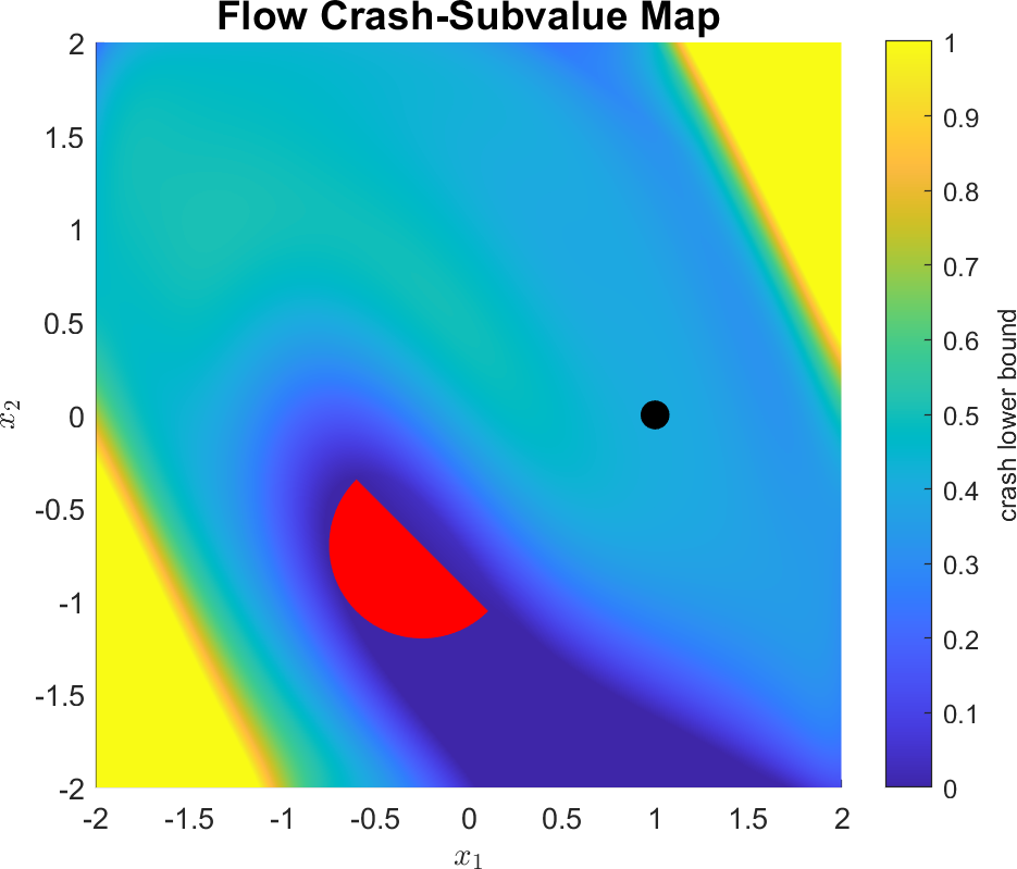
Figure 2: Subvalue function for Flow system (7) between degrees $1..5$.

The black dot in Figure 2 is the specific initial point $X_{0}=[1;0]$. Table 1 lists crash-bounds on (7) starting at $X_{0}$. The subvalue bound (27) is lower than the corresponding degree bounds at the $X_{0}$-specific program (11).

Table 1: Crash-bounds at $X_{0}=[1;0]$ under SOS tightenings

order	1	2	3	4	5
subvalue (27)	$1.089\times 10^{-9}$	$1.607\times 10^{-9}$	0.1473	0.3392	0.4053
specific (11)	$1.117\times 10^{-7}$	0.1843	0.4369	0.5092	0.5118

We now consider worst-case crash-bounds for the half-circle set with respect to the perturbed flow system (7) and the circular initial set $X_{0}=\{x\mid 0.4^{2}\geq(x_{1}-1)^{2}+x_{2}\}$. Crash-bounds as computed by (23) (SOS tightenings to (11)) in degrees $1..5$ are $[8.101\times 10^{-8},6.590\times 10^{-2},0.4054,0.4631,0.4638].$ The degree-5 lower-bound of $0.4638$ should be compared against the numerical bound of $0.4639$ produced by CasADi. The numerically solved trajectory (blue curve) is plotted in Figure 3, along with the unsafe set $X_{u}$ (red half-circle) and the initial set $X_{0}$ (black circle). The initial point of the controlled trajectory (blue dot) is $x_{0}\approx[1.3424;0.2069]$.

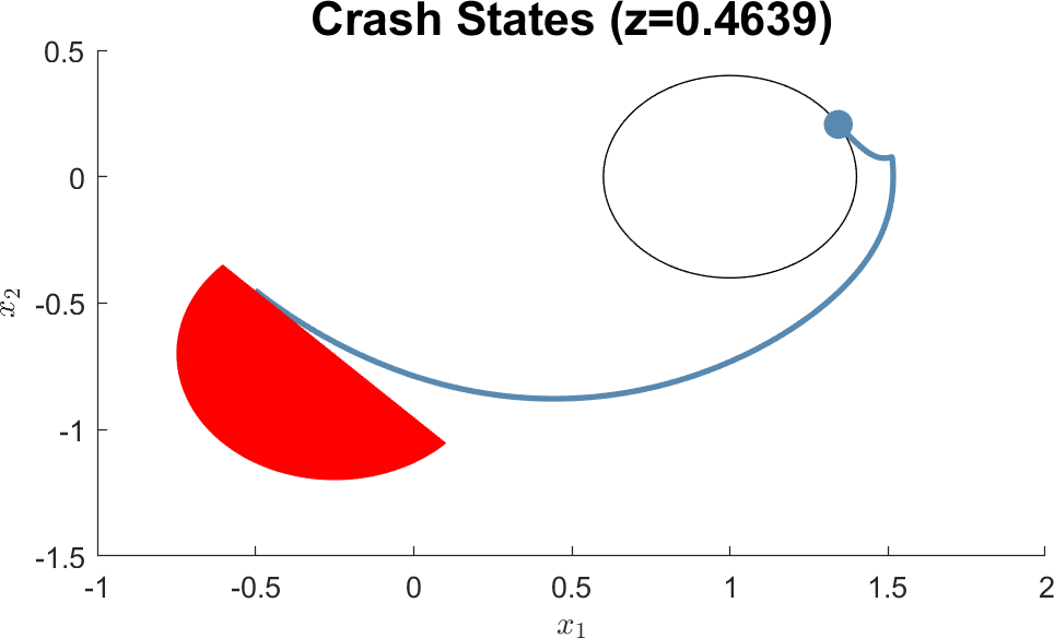
Figure 3: Numerical optimal control yields worst-case $Q^{*}\approx 0.4639$ for the half-circle $X_{u}$

7.1.2 Moon

The second part of this example has a nonconvex moon-shaped unsafe set

$$X_{u}=\{x\mid 0.8^{2}-(x_{1}-0.4)^{2}-(x_{2}+0.4)^{2}\geq 0,\ (x_{1}-0.6596)^{2}+(x_{2}-0.3989)^{2}-1.16^{2}\geq 0\}.$$ (32)

Figure 4 displays a controlled trajectory (blue curve) starting from $X_{0}=[0;0]$ (black circle) and terminating in the $X_{u}$ (red moon), as computed by CasADi.

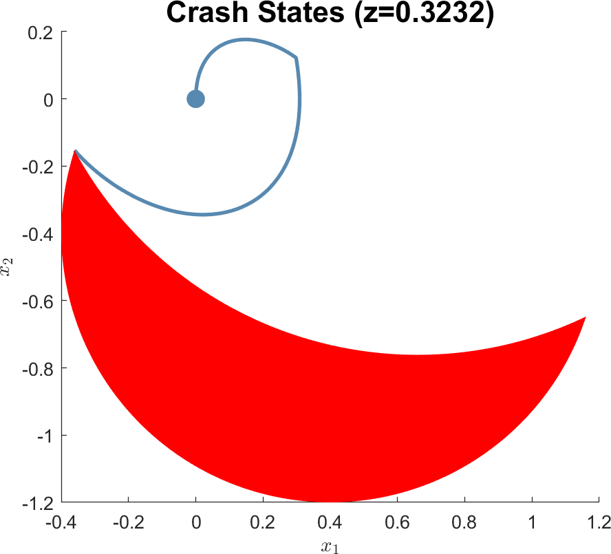
Figure 4: Numerical optimal control yields $Q^{*}\approx 0.3232$ for the moon $X_{u}$

Table 2 lists subvalue (27) and specific (11) crash-bounds for $X_{0}=[0;0]$ between degrees $1..5$. The objectives of the SOS tightenings to (27) are $J^{*}_{1..5}=[1.973\times 10^{-7},1.323\times 10^{-7},1.027,3.188,4.502]$.

Table 2: Crash-bounds at $X_{0}=[0;0]$ for the moon (32) under SOS tightenings

order	1	2	3	4	5
subvalue (27)	$8.770\times 10^{-9}$	$4.652\times 10^{-10}$	$-7.861\times 10^{-2}$	$-5.692\times 10^{-3}$	$7.721\times 10^{-2}$
specific (11)	$2.723\times 10^{-8}$	0.1010	0.2912	0.3216	0.3224

Figure 5 plots the subvalue function $q_{1:5}(x)$ from (30) under a cap of $Q_{\max}=2$ (and $J_{\max}=1$). All values of $q_{1:5}$ in Figure 5 are clamped to $[0,J_{\max}]$.

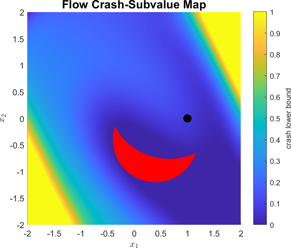
Figure 5: Subvalue map for the moon (32) on the flow system (7)

7.2 Data-Driven Flow System

Data $\mathcal{D}$ is collected for the Flow system (6) from $N_{s}=40$ samples with perfect knowledge in dynamics $\dot{x}_{1}=x_{2}$ and a ground-truth noise bound of $\epsilon=0.5$ in the coordinate $\dot{x}_{2}$. The noisy derivative data in $\mathcal{D}$ and ground-truth derivatives are drawn in the orange and blue arrows respectively in Figure 6. It is assumed that $\dot{x}_{2}$ is described by a cubic polynomial in $(x_{1},x_{2})$. The parameterized polytope $\{w\mid Aw\leq b+z\}$ ($\Omega$ with fixed $z$ value) has $L=10$ dimensions and $m=2nT=80$. The minimum possible corruption while obeying (14) under the cubic noise model is $\inf_{(w,z)\in\Omega}z=0.4617$.

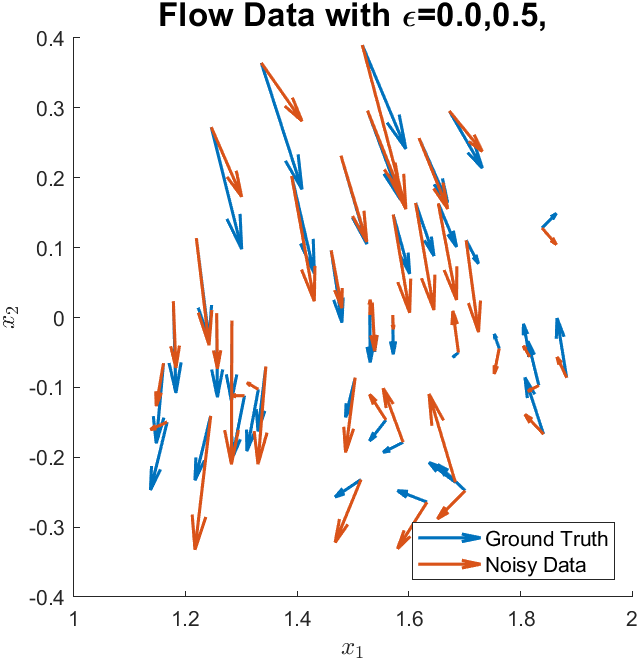
Figure 6: Observed data of the Flow system (6)

The crash-safety problem (11) and subvalue problem (27) were solved with the unsafe set $X_{u}=\{x\mid(x_{1}+0.25)^{2}+(x_{2}+0.7)^{2}\leq 0.5^{2},\ (0.95+x_{1}+x_{2})/\sqrt{2}\leq 0\}$ between $t=[0,5]$ time units in the space $X=\{x\in\mathbb{R}^{2}:\lVert x\rVert_{2}^{2}\leq 8\}$. The subvalue problem (27) integrates over the uniform measure of the ball $X$.

Table 3 reports bounds for the crash-corruption $Q(X_{0})$ by solving Lie-robustified SOS tightenings of (11) and (27) from degrees $1..4$ with $J_{\max}=1,\ Q_{\max}=4$. The objective function (integrals of $q(x)$) for the subvalue (27) are $J^{*}_{1:4}=[0.2193,3.8185,7.8326,18.5945]$. The subvalue-estimated control cost at $X_{0}$ between degrees $1..4$ is $0.3399$ by Equation (30). The subvalue-estimated bound is valid for all $x\in X$, and is therefore lower than the bound $q^{*}_{4}=0.5499$ from (11) that focuses exclusively on the initial point $X_{0}$.

Table 3: Data-Driven Crash-bounds at $X_{0}=[1;0]$ under SOS tightenings

order	1	2	3	4
specific (11)	$0.0582$	$0.4423$	0.4864	0.5499
subvalue (27)	$6.180\times 10^{-3}$	0.1829	0.3399	-19.01

Figure 7 plots the subvalue function from (30) on the data-driven flow system. Subvalues in the plot are clamped to the range $[0,J_{\max}]=[0,1]$.

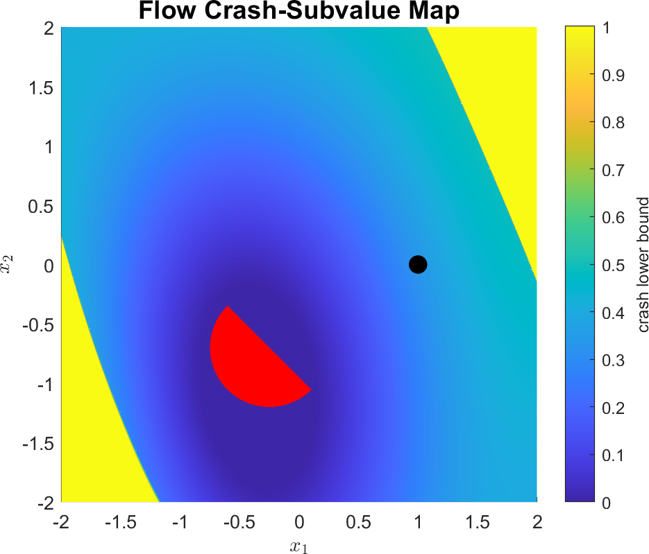
Figure 7: Subvalue for data-driven (6) between degrees $1..4$

Safety of trajectories starting in $X_{0}$ is certified because the crash-bound $\tilde{q}^{*}_{4}=0.5499$ is greater than the ground-truth noise-bound $\epsilon=0.5$. Figure 8 uses the CasADi optimal control suite [28] to numerically solve the crash program (1). The numerical crash-bound of $q^{\textrm{CasADI}}=0.5499$ is approximately equal (up to four decimal places) to the crash-bound $q^{*}_{4}=0.5499$.

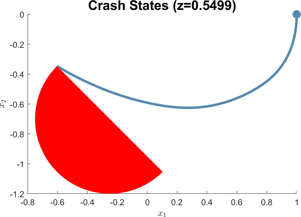
Figure 8: Numerically computed crash-bound for data-driven Flow (6)

The left plot of figure 9 shows the applied control of the $L=10$ inputs. The right plot demonstrates how the polytopic input constraint is obeyed with respect to the crash bound $q^{\textrm{CasADI}}=0.5499$ (upper and lower black lines).

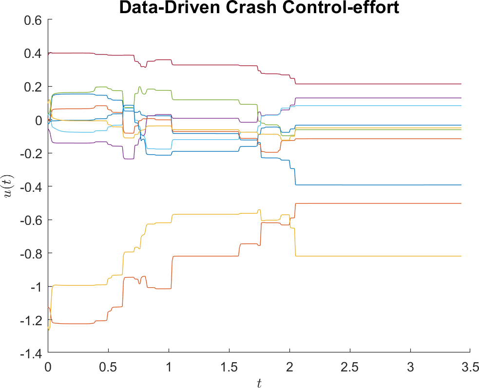
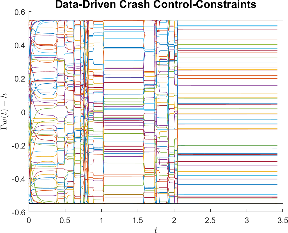
Figure 9: Applied control for the data-driven Flow crash system.

These crash-bounds should be compared against the $L_{2}$ distance estimates of $c^{*}_{1:5}=[1.698\times 10^{-5},\ 0.1936,\$ $0.2003,\ 0.2009,\ 0.2013]$ from Section 6.3 of [21]. The distance estimates do not indicate that adding an additional budget of $0.0499$ constraint violation will cause at least one trajectory to enter the unsafe set.

8 Conclusion

This paper utilized peak minimizing control in order to perform safety analysis. The returned values from SOS programs are lower-bounds on the maximal control effort needed to crash into the unsafe set. Crash-safety adds a new perspective on the safety of trajectories, covering some of the blind spots of distance estimation and safety margins. Crash-safety may be applied in the context of data-driven systems analysis, by quantifying the minimum tolerable corruption in a noise model before a trajectory is at risk of being unsafe.

Future work involves attempting to reduce computational burden of the Crash programs (22) by identifying new kinds of structure (in addition to robust decompositions) to hopefully allow for real-time computation. Other extensions could include applying these methods to other classes of systems (e.g., discrete-time, hybrid), and creating a stochastic interpretation of crash-safety.

References

- [1] R. B. Vinter, “Minimax optimal control,” SIAM journal on control and optimization, vol. 44, no. 3, pp. 939–968, 2005.
- [2] E. Molina and A. Rapaport, “An optimal feedback control that minimizes the epidemic peak in the sir model under a budget constraint,” Automatica, vol. 146, p. 110596, 2022.
- [3] P. Lu and N. X. Vinh, “Minimax optimal control for atmospheric fly-through trajectories,” Journal of Optimization Theory and Applications, vol. 57, no. 1, pp. 41–58, 1988.
- [4] H. Kreim, B. Kugelmann, H. J. Pesch, and M. H. Breitner, “Minimizing the Maximum Heating of a Reentering Space Shuttle: An Optimal Control Problem with Multiple Control Constraints,” Optimal Control Applications and Methods, vol. 17, no. 1, pp. 45–69, 1996.
- [5] E. Molina, A. Rapaport, and H. Ramírez, “Equivalent Formulations of Optimal Control Problems with Maximum Cost and Applications,” Journal of Optimization Theory and Applications, vol. 195, no. 3, pp. 953–975, 2022.
- [6] S. Prajna and A. Jadbabaie, “Safety Verification of Hybrid Systems Using Barrier Certificates,” in International Workshop on Hybrid Systems: Computation and Control. Springer, 2004, pp. 477–492.
- [7] S. Prajna, “Barrier certificates for nonlinear model validation,” Automatica, vol. 42, no. 1, pp. 117–126, 2006.
- [8] A. Rantzer and S. Prajna, “On Analysis and Synthesis of Safe Control Laws,” in 42nd Allerton Conference on Communication, Control, and Computing. University of Illinois, 2004, pp. 1468–1476.
- [9] J. Miller, D. Henrion, and M. Sznaier, “Peak Estimation Recovery and Safety Analysis,” IEEE Control Systems Letters, vol. 5, no. 6, pp. 1982–1987, 2020.
- [10] J. Miller and M. Sznaier, “Bounding the Distance to Unsafe Sets with Convex Optimization,” 2021, arXiv: 2110.14047.
- [11] D. Liberzon, Calculus of Variations and Optimal Control Theory: A Concise Introduction. Princeton university press, 2011.
- [12] R. Lewis and R. Vinter, “Relaxation of Optimal Control Problems to Equivalent Convex Programs,” Journal of Mathematical Analysis and Applications, vol. 74, no. 2, pp. 475–493, 1980.
- [13] D. Henrion, J. B. Lasserre, and C. Savorgnan, “Nonlinear optimal control synthesis via occupation measures,” in 2008 47th IEEE Conference on Decision and Control. IEEE, 2008, pp. 4749–4754.
- [14] D. Henrion and M. Korda, “Convex Computation of the Region of Attraction of Polynomial Control Systems,” IEEE TAC, vol. 59, no. 2, pp. 297–312, 2013.
- [15] M. Korda, D. Henrion, and C. N. Jones, “Inner approximations of the region of attraction for polynomial dynamical systems,” IFAC Proceedings Volumes, vol. 46, no. 23, pp. 534–539, 2013.
- [16] G. Fantuzzi and D. Goluskin, “Bounding Extreme Events in Nonlinear Dynamics Using Convex Optimization,” SIAM Journal on Applied Dynamical Systems, vol. 19, no. 3, pp. 1823–1864, 2020.
- [17] J. Miller, D. Henrion, M. Sznaier, and M. Korda, “Peak Estimation for Uncertain and Switched Systems,” in 2021 60th IEEE Conference on Decision and Control (CDC), 2021, pp. 3222–3228.
- [18] M. Korda, D. Henrion, and C. N. Jones, “Convex computation of the maximum controlled invariant set for polynomial control systems,” SIAM Journal on Control and Optimization, vol. 52, no. 5, pp. 2944–2969, 2014.
- [19] J. B. Lasserre, Moments, Positive Polynomials And Their Applications, ser. Imperial College Press Optimization Series. World Scientific Publishing Company, 2009.
- [20] A. Ben-Tal, L. El Ghaoui, and A. Nemirovski, Robust Optimization. Princeton University Press, 2009, vol. 28.
- [21] J. Miller and M. Sznaier, “Analysis and Control of Input-Affine Dynamical Systems using Infinite-Dimensional Robust Counterparts,” 2023, arxiv:2112.14838.
- [22] D. Hilbert, “Über die darstellung definiter formen als summe von formenquadraten,” Mathematische Annalen, vol. 32, no. 3, pp. 342–350, 1888.
- [23] F. Alizadeh, “Interior Point Methods in Semidefinite Programming with Applications to Combinatorial Optimization,” SIAM J OPTIMIZ, vol. 5, no. 1, pp. 13–51, 1995.
- [24] J. Miller, T. Dai, and M. Sznaier, “Data-Driven Superstabilizing Control of Error-in-Variables Discrete-Time Linear Systems,” in 2022 61st IEEE Conference on Decision and Control (CDC), 2022, pp. 4924–4929.
- [25] M. Putinar, “Positive Polynomials on Compact Semi-algebraic Sets,” Indiana University Mathematics Journal, vol. 42, no. 3, pp. 969–984, 1993.
- [26] J. Nie and M. Schweighofer, “On the complexity of Putinar’s Positivstellensatz,” Journal of Complexity, vol. 23, no. 1, pp. 135–150, 2007.
- [27] J. Cimprič, M. Marshall, and T. Netzer, “Closures of quadratic modules,” Israel Journal of Mathematics, vol. 183, no. 1, pp. 445–474, 2011.
- [28] J. A. Andersson, J. Gillis, G. Horn, J. B. Rawlings, and M. Diehl, “CasADi: a software framework for nonlinear optimization and optimal control,” Mathematical Programming Computation, vol. 11, pp. 1–36, 2019.
- [29] L. C. Young, “Generalized Surfaces in the Calculus of Variations,” Annals of mathematics, vol. 43, pp. 84–103, 1942.
- [30] J. B. Lasserre, D. Henrion, C. Prieur, and E. Trélat, “Nonlinear Optimal Control via Occupation Measures and LMI-Relaxations,” SIAM Journal on Control and Optimization, vol. 47, no. 4, pp. 1643–1666, 2008.
- [31] M. Tacchi, “Convergence of Lasserre’s hierarchy: the general case,” Optimization Letters, vol. 16, no. 3, pp. 1015–1033, 2022.
- [32] M. Jones and M. M. Peet, “Polynomial Approximation of Value Functions and Nonlinear Controller Design with Performance Bounds,” 2021.
- [33] R. Caron, J. McDonald, and C. Ponic, “A degenerate extreme point strategy for the classification of linear constraints as redundant or necessary,” Journal of Optimization Theory and Applications, vol. 62, no. 2, pp. 225–237, 1989.
- [34] V. Loechner and D. K. Wilde, “Parameterized polyhedra and their vertices,” International Journal of Parallel Programming, vol. 25, pp. 525–549, 1997.
- [35] J. B. Lasserre, “A “Joint+Marginal” Approach to Parametric Polynomial Optimization,” SIAM Journal on Optimization, vol. 20, no. 4, pp. 1995–2022, 2010.
- [36] D. Gottlieb and C.-W. Shu, “On the Gibbs phenomenon and its resolution,” SIAM review, vol. 39, no. 4, pp. 644–668, 1997.
- [37] M. Tacchi, J. B. Lasserre, and D. Henrion, “Stokes, Gibbs, and Volume Computation of Semi-Algebraic Sets,” Discrete & Computational Geometry, pp. 1–24, 2022.
- [38] J. Lofberg, “YALMIP : a toolbox for modeling and optimization in MATLAB,” in ICRA (IEEE Cat. No.04CH37508), 2004, pp. 284–289.
- [39] M. ApS, The MOSEK optimization toolbox for MATLAB manual. Version 9.2., 2020. [Online]. Available: https://docs.mosek.com/9.2/toolbox/index.html