An implicit function theorem for the stream calculus

Abstract

In the context of the stream calculus, we present an Implicit Function Theorem (IFT) for polynomial systems, and discuss its relations with the classical IFT from calculus. In particular, we demonstrate the advantages of the stream IFT from a computational point of view, and provide a few example applications where its use turns out to be valuable.

1 Introduction

In theoretical computer science, the last two decades have seen an increasing interest in the concept of stream and in the related proof techniques, collectively designated as the stream calculus [22, 23, 25]. A stream $\sigma=(r_{0},r_{1},...)$ is an infinite sequence of elements (coefficients) $r_{i}$ drawn from any set; the stream calculus requires that this set be endowed with some algebraic structure, such as a field. Therefore, as a concrete mathematical object, a stream is just the same as a formal power series considered in combinatorics and other fields of mathematics. The use of a different terminology here is motivated by the fact that, with streams, the basic computational device is that of stream derivative, as opposed to the ordinary derivative from calculus considered in formal power series. The stream derivative $\sigma^{\prime}$ is obtained by simply removing the first element $r_{0}$ from $\sigma$. The ordinary derivative of a formal power series, on the other hand, does not enjoy such a simple formulation in terms of stream manipulation. The simplicity of stream derivative also leads to computational advantages, as discussed further below. Algebraically, the stream derivative enjoys a nice relation with the operation of convolution $\times$ (one of the possible notions of product for streams, to be introduced in Section 2), as expressed by the so-called fundamental theorem of the stream calculus:

$$\sigma=\sigma(0)+X\times\sigma^{\prime}\,.$$

Here, $\sigma(0)$ is taken as an abbreviation of the stream $(\sigma(0),0,0,...)$, while $X=(0,1,0,0,...)$. As can be intuited from this equation, multiplying a stream ($\sigma^{\prime}$ in this case) by $X$ has the effect of shifting one position to the left the stream’s coefficients.

A powerful and elegant proof technique for streams is coinduction [27], whose step-by-step flavour naturally agrees with the above mentioned features of streams, in particular stream derivative. Moreover, an important specification and computational device is represented by stream differential equations (SDEs, [13]), the analog of ordinary differential equations (ODEs) for functions and formal power series [10, 30]. It is this toolkit of mechanisms and proof techniques that one collectively designates as the stream calculus [22, 23, 25]. One point of strength of the stream calculus is that it provides simple, direct and unified reasoning techniques, that can be applied to a variety of systems that involve the treatment of sequences. A distinguished feature of proofs conducted within the stream calculus is that issues related to convergence (of sequences, functions etc.) basically never enter the picture. As an example, the stream calculus has been proved valuable in providing a coinductive account of analytic functions and Laplace transform [19], in solving difference and differential equations [5, 6, 23, 25], as well as in formalizing several versions of signal flow graphs [3, 4, 24, 26]. In Section 2, we provide a quick overview of the basic definitions and features of the stream calculus.

The main goal and contribution of the present work is to add yet another tool to the stream calculus: an Implicit Function Theorem (IFT) for systems of stream polynomial equations. Indeed, while SDEs represent a powerful computational device, depending on the problem at hand, streams may be more naturally expressed in an algebraic fashion, that is as the (unique) solution of systems of polynomial equations. In analogy with the classical IFT from calculus [15, 21, 28], our main result provides sufficient syntactic conditions under which a system of polynomial equations has a unique stream solution. Moreover, the theorem also provides an equivalent system of SDEs, that is useful to actually generate the stream solution. It is here that the computational advantage of stream derivatives, as opposed to ordinary ones, clearly shows up.

In the classical IFT [21, Th.9.28], one considers a system of equations in the variables $(x,{\boldsymbol{\mathrm{y}}})$, say ${\boldsymbol{\mathrm{F}}}(x,{\boldsymbol{\mathrm{y}}})=0$; for simplicity, here we assume that $x$ is a scalar, while ${\boldsymbol{\mathrm{y}}}$ can be a vector. The IFT gives sufficient conditions under which, for any fixed point $(x_{0},{\boldsymbol{\mathrm{y}}}_{0})$ satisfying ${\boldsymbol{\mathrm{F}}}(x_{0},{\boldsymbol{\mathrm{y}}}_{0})=0$, a neighbourhood around $x_{0}$ and a map $f$ on that neighbourhood exist fulfilling $f(x_{0})={\boldsymbol{\mathrm{y}}}_{0}$ and ${\boldsymbol{\mathrm{F}}}(x,f(x))=0$. Otherwise said, ${\boldsymbol{\mathrm{F}}}(x,{\boldsymbol{\mathrm{y}}})=0$ implicitly defines a function $f$ (hence the name of the theorem) such that $f(x_{0})={\boldsymbol{\mathrm{y}}}_{0}$ and ${\boldsymbol{\mathrm{F}}}(x,f(x))$ is identically 0 in a neighborhood of $x_{0}$, The required sufficient condition is that the Jacobian matrix (the matrix of partial derivatives) of ${\boldsymbol{\mathrm{F}}}$ with respect to ${\boldsymbol{\mathrm{y}}}$ be nonsingular when evaluated at $(x_{0},{\boldsymbol{\mathrm{y}}}_{0})$. The theorem also gives a system of ODEs whose solution is the function $f(x)$. Although the ODE  system will be in general impossible to solve analytically, it can be used to compute a truncated Taylor series of $f(x)$ to the desired degree of approximation.

In Section 3, in the setting of the stream calculus and of polynomial equations, we obtain a version of the IFT whose form closely resembles the classical one (Theorem 3.1). The major difference is that the stream version relies, of course, on stream derivatives, and on a corresponding notion of stream Jacobian. In particular, the system of ODEs that defines the solution is here replaced by a system of SDEs. A crucial step towards proving the result is devising a stream version of the chain rule from calculus, whereby one can express the derivative of a function ${\boldsymbol{\mathrm{F}}}(x,y_{1}(x),...,y_{n}(x))$ with respect to $x$ in terms of the partial derivatives of ${\boldsymbol{\mathrm{F}}}$ with respect to $y_{i}$ and the ordinary derivative of the $y_{i}$ with respect to $x$.

In Section 4, beyond the formal similarity, we discuss the precise mathematical relation of the stream IFT with the classical IFT (Theorem 4.1). We show that the two theorems can be applied precisely under the same assumptions on the classical Jacobian of ${\boldsymbol{\mathrm{F}}}(x,{\boldsymbol{\mathrm{y}}})$. Moreover, the sequence of Taylor coefficients of the function defined by the classical IFT coincides with the solution identified by the stream IFT. Therefore, one has two alternative methods to compute the (stream) solution. Despite this close relationship, the stream version of the theorem is conceptually and computationally very different from the classical one; the computational aspects will be further discussed below. In Section 4, we also discuss the relation of the stream IFT with algebraic series as considered in enumerative combinatorics [10, 30].

As an extended example of application of the stream IFT, in Section 5 we apply the result to the problem of enumerating three-colored trees [10, Sect.4, Example 14], a typical class of combinatorial objects that are most naturally described by algebraic equations.

In Section 6 we discuss the computational aspects of the stream IFT. We first outline an efficient method to calculate the coefficients of the stream solution up to a prescribed order, based on the SDE system provided by the theorem. Then we offer an empirical comparison between two methods to compute the stream solution: the above mentioned method based on the stream IFT, and the method based on the ODEs provided by the classical IFT. This comparison clearly shows the computational benefits of first method (stream IFT) over the second one (classical IFT) in terms of running time. An important point is that, when applied to polynomials, the syntactic size of stream derivatives is approximately half the size of ordinary (classical) derivatives.

We conclude the paper in Section 7 with a brief discussion on possible directions for future research.

Related work

The stream calculus in the form considered here has been introduced by Rutten in a series of works, in particular [22] and [23]. In [22], streams and operators on streams are introduced via coinductive definitions and behavioural differential equations, later called stream differential equations, involving initial conditions and derivatives of streams. Several applications are also presented to: difference equations, analytical differential equations, and some problems from discrete mathematics and combinatorics. In [23] streams, automata, languages and formal power series are studied in terms of the notions of coalgebra homomorphisms and bisimulation.

A recent development of the stream calculus that is related to the present work is [7], where the authors introduce a polynomial format for SDEs  and an algorithm to automatically check polynomial equations, with respect to a generic notion of product for streams satisfying certain conditions. These results can be applied to convolution and shuffle products, among the others.

In formal language theory, context-free grammars can be viewed as instances of polynomial systems: see [16]. A coinductive treatment of this type of systems is found in Winter’s work [31, Ch.3]. Note that, on one hand, the polynomial format we consider here is significantly more expressive than context-free grammars, as we can deal with such equations as $x^{2}+y^{2}-1=0$ (see Example 3 in Section 3) that are outside the context-free format. On the other hand, here we confine to univariate streams, which can be regarded as weighted languages on the alphabet $\{x\}$, whereas in language theory alphabets of any finite size can be considered. How to extend the present results to multivariate streams is a challenging direction for future research.

In enumerative combinatorics [10, 30], formal power series defined via polynomial equations are named algebraic series. [10, Sect.4] discusses several aspects of algebraic series, including several methods of reduction, involving the theory of resultants and Groebner bases. We compare our approach to algebraic series in Section 3, Remark 3.

2 Background

2.1 Streams

Let $(\mathbb{K},0,1,+,\cdot)$ be a field. We let $\Sigma\langle\mathbb{K}\rangle:=\mathbb{K}^{\omega}$, ranged over by $\sigma,\tau,...$, denote the set of streams, that are infinite sequences of elements from $\mathbb{K}$: $\sigma=(r_{0},r_{1},r_{2},...)$ with $r_{i}\in\mathbb{K}$. Often $\mathbb{K}$ is understood from the context and we shall simply write $\Sigma$ rather than $\Sigma\langle\mathbb{K}\rangle$. When convenient, we shall explicitly consider a stream $\sigma$ as a function from $\mathbb{N}$ to $\mathbb{K}$ and, e.g., write $\sigma(i)$ to denote the $i$-th element of $\sigma$. By slightly overloading the notation, and when the context is sufficient to disambiguate, the stream $(r,0,0,...)$ ($r\in\mathbb{K}$) will be simply denoted by $r$, while the stream $(0,1,0,0,...)$ will be denoted by $X$; see [23] for motivations behind these notations. Given two streams $\sigma$ and $\tau$, we define the streams $\sigma+\tau$ (sum) and $\sigma\times\tau$ (convolution product) by

$$(\sigma+\tau)(i) :=\sigma(i)+\tau(i) (\sigma\times\tau)(i) :=\sum_{0\leq j\leq i}\sigma(j)\cdot\tau(i-j)$$ (1)

for each $i\geq 0$, where the $+$ and $\cdot$ on the right-hand sides above denote sum and product in $\mathbb{K}$, respectively. Sum enjoys the usual commutativity and associativity properties, and has the stream $0=(0,0,...)$ as an identity. Convolution product is commutative, associative, has $1=(1,0,0,...)$ as an identity, and distributes over $+$; differently from, e.g., [7, 13], here we only consider the convolution product. Multiplication of $\sigma=(r_{0},r_{1},...)$ by a scalar $r\in\mathbb{K}$, denoted $r\sigma=(r\,r_{0},r\,r_{1},...)$, is also defined and makes $(\Sigma,+,0)$ a vector space over $\mathbb{K}$. Therefore, $(\Sigma,+,\times,0,1)$ forms a (associative) $\mathbb{K}$-algebra. We also record the following facts for future use: $X\times\sigma=(0,\sigma(0),\sigma(1),...)$ and $r\,\times\,\sigma=(r\,\sigma(0),r\,\sigma(1),...)$, where $r\in\mathbb{K}$. In view of the second equation above, $r\,\times\,\sigma$ coincides with $r\sigma$.

For each $\sigma$, we let its derivative $\sigma^{\prime}$ be the stream defined by $\sigma^{\prime}(i)=\sigma(i+1)$ for each $i\geq 0$. In other words, $\sigma^{\prime}$ is obtained from $\sigma$ by removing the first element $\sigma(0)$. The equality $X\times\sigma=(0,\sigma(0),\sigma(1),...)$ above leads to the so called fundamental theorem of the stream calculus, whereby for each $\sigma\in\Sigma$

$$\sigma=\sigma(0)+X\times\sigma^{\prime}\,.$$ (2)

Every stream $\sigma$ such that $\sigma(0)\neq 0$ has a unique inverse with respect to convolution, denoted $\sigma^{-1}$, that satisfies the equations:

$$(\sigma^{-1})^{\prime} =-\sigma(0)^{-1}\cdot(\sigma^{\prime}\times\sigma^{-1}) (\sigma^{-1})(0) =\sigma(0)^{-1}\,.$$ (3)

2.2 Polynomial stream differential equations

Let us fix a finite, non empty set of symbols or variables $\mathcal{Y}=\{y_{1},\ldots,y_{n}\}$ and a distinguished variable $x\notin\mathcal{Y}$. Notationally, when fixed an order on such variables, we use the notation ${\boldsymbol{\mathrm{y}}}:=(y_{1},...,y_{n})$. We fix a generic field $\mathbb{K}$ of characteristic 0; $\mathbb{K}=\mathbb{R}$ and $\mathbb{K}=\mathbb{C}$ will be typical choices. We let ${\cal P}:=\mathbb{K}[x,y_{1},...,y_{n}]$, ranged over by $p,q,...$, be the set of polynomials with coefficients in $\mathbb{K}$ and indeterminates in $\{x\}\cup\mathcal{Y}$. As usual, we shall denote polynomials as formal finite sums of distinct monomials with coefficients in $\mathbb{K}$: $p=\sum_{i\in I}r_{i}m_{i}$, for $r_{i}\in\mathbb{K}$ and $m_{i}$ monomials over $\{x\}\cup\mathcal{Y}$. For the sake of uniform notation, we shall sometimes let $y_{0}$ denote $x$, so we can write a generic monomial in ${\cal P}$ as $y_{0}^{k_{0}}\cdots y_{n}^{k_{n}}$, for $k_{i}\in\mathbb{N}$ for every $i$. By slight abuse of notation, we shall write the zero polynomial and the empty monomial as $0$ and $1$, respectively.

Over ${\cal P}$, one defines the usual operations of sum $p+q$ and product $p\cdot q$, with 0 and 1 as identities, and enjoying commutativity, associativity and distributivity, which make ${\cal P}$ a ring. Multiplication of $p\in{\cal P}$ by a scalar $r\in\mathbb{K}$, denoted $rp$, is also defined and makes $({\cal P},+,0)$ a vector space over $\mathbb{K}$. Therefore, $({\cal P},+,\times,0,1)$ as well forms a free $\mathbb{K}$-algebra with generators $(x,y_{1},...,y_{n})$. For each $n$-tuple of streams ${\boldsymbol{\mathrm{\sigma}}}=(\sigma_{1},...,\sigma_{n})$, there is a unique $\mathbb{K}$-algebra homomorphism $\phi_{{\boldsymbol{\mathrm{\sigma}}}}:{\cal P}\longrightarrow\Sigma$ such that $\phi_{{\boldsymbol{\mathrm{\sigma}}}}(x)=X$ and $\phi_{{\boldsymbol{\mathrm{\sigma}}}}(y_{i})=\sigma_{i}$ for $i=1,...,n$. For any $p\in{\cal P}$, we let $p(X,{\boldsymbol{\mathrm{\sigma}}}):=\phi_{{\boldsymbol{\mathrm{\sigma}}}}(p)$, that is the result of substituting the variables $x$ and ${\boldsymbol{\mathrm{y}}}$ in $p$ with the streams $X$ and ${\boldsymbol{\mathrm{\sigma}}}$, respectively.

Definition 1 (SDE [23]).

Given a tuple of polynomials $(p_{1},...,p_{n})\in{\cal P}^{n}$ and ${\boldsymbol{\mathrm{r}}}_{0}=(r_{1},...,r_{n})\in\mathbb{K}^{n}$, the corresponding system of (polynomial) stream differential equations (SDEs) $\mathcal{D}$ and initial conditions are written as follows

$$\mathcal{D} =\{y^{\prime}_{1}=p_{1},...,y^{\prime}_{n}=p_{n}\} \rho=\{y_{1}(0)=r_{1},...,y_{n}(0)=r_{n}\}\,.$$ (4)

The pair $(\mathcal{D},\rho)$ is also said to form a (polynomial) SDE initial value problem for the variables ${\boldsymbol{\mathrm{y}}}$. A solution of (4) is a tuple of streams ${\boldsymbol{\mathrm{\sigma}}}=(\sigma_{1},...,\sigma_{n})\in\Sigma^{n}$ such that $\sigma^{\prime}_{i}=p_{i}(X,{\boldsymbol{\mathrm{\sigma}}})$ and $\sigma_{i}(0)=r_{i}$, for $i=1,...,n$.

A natural generalization of the above definition are systems of rational SDEs, where the right-hand side of each equation is a fraction of polynomials. Systems of rational SDEs have indeed the same expressive power as polynomial ones: a version of this (well-known) result will be explicitly formulated in Section 3 (see Lemma 3.2). For a proof of the following theorem (in a more general context), see e.g. [7, 13].

Theorem 2.1 (existence and uniqueness of solutions).

Every polynomial SDE initial value problem of the form (4) has a unique solution.

Remark 1 (stream coefficients computation).

We record for future use that a SDE initial value problem $(\mathcal{D},\rho)$ like (4) yields a recurrence relation, hence an algorithm, to compute the coefficients of the solution streams $\sigma_{i}$. Indeed, denote by $\sigma_{:k}$ the stream that coincides with $\sigma$ when restricted to $\{0,...,k\}$ and is 0 elsewhere. This notation is extended to a tuple ${\boldsymbol{\mathrm{\sigma}}}$ componentwise. Then we have, for each $i=1,...,n$ and $k\geq 0$:

$$\sigma_{i}(0) =y_{i}(0)$$ (5)

$$\sigma_{i}(k+1) =\sigma^{\prime}_{i}(k)\,=\,p_{i}(X,{\boldsymbol{\mathrm{\sigma}}})(k)\,=\,p_{i}(X,{\boldsymbol{\mathrm{\sigma}}}_{:k})(k)$$ (6)

where the last step follows from the fact that the $k$-th coefficient of $p_{i}(X,{\boldsymbol{\mathrm{\sigma}}})$ only depends on the first $k$ coefficients of ${\boldsymbol{\mathrm{\sigma}}}$ (see (1)). In the literature, this is referred to as causality (see [13, 14, 20], just to cite a few).

As an example, consider (here we let $y=y_{1}$):

$$y^{\prime}=y^{2}\qquad\qquad y(0)=1$$

for which we get the recurrence: $\sigma(0)=1$ and $\sigma(k+1)=\sigma^{2}(k)=\sum_{j=0}^{k}\sigma(j)\cdot\sigma(k-j)$. From the computational point of view this is far from optimal. Indeed, in the case of a single polynomial equation ($n=1$) like this one, a linear (in $y$) recurrence relation for generating the Taylor coefficients of the solution can always be efficiently built; see [10, 30]. In the case of $n>1$ equations, the situation is more complicated. We defer to Section 6 further considerations on the computation of stream coefficients, including details on an effective implementation of (6).

3 An implicit function theorem for the stream calculus

Let $\mathcal{E}\subseteq{\cal P}$ be a finite, nonempty set of polynomials that we call polynomial system. A stream solution of $\mathcal{E}$ is a tuple of streams ${\boldsymbol{\mathrm{\sigma}}}=(\sigma_{1},...,\sigma_{n})$ such that $p(X,{\boldsymbol{\mathrm{\sigma}}})=0$ for each $p\in\mathcal{E}$. We want to show that, under certain syntactic conditions, $\mathcal{E}$ has a unique stream solution, which can be also defined via a polynomial SDE initial value problem $(\mathcal{D},\rho)$. Instrumental to establish this result is a close stream analog of the well known Implicit Function Theorem (IFT) from calculus.

Let us introduce some extra notation on polynomials and streams. Beside the variables $x$ and ${\boldsymbol{\mathrm{y}}}=(y_{1},...,y_{n})$, we shall consider a set of new, distinct initial value indeterminates ${\boldsymbol{\mathrm{y}}}_{0}=(y_{01},...,y_{0n})$ and primed indeterminates ${\boldsymbol{\mathrm{y^{\prime}}}}=(y^{\prime}_{1},...,y^{\prime}_{n})$. As usual, we let $y_{0}=x$; moreover, by slightly abusing notation, we will let $y_{00}$ denote $0$ (the scalar zero). We will assume a fixed total order on all variables $(x=)y_{0}<y_{1}<\cdots<y_{n}$ and, for any monomial $m\neq 1$, on the variables in ${\boldsymbol{\mathrm{y}}}$ define $\min(m):=\min\{y\,:\,y\text{ occurs in }m\}$, where the $\min$ is taken according to the fixed total order on variables. In the definition below, we order the individual variables in a monomial according to $<$ before proceeding to differentiation. It will turn out that the chosen total order is semantically immaterial, see Remark 2 further below. The total degree of a monomial $m$ is just its size, that is the number of occurrences of variables in $m$. Recall that $\mathbb{K}[x,{\boldsymbol{\mathrm{y}}}_{0},{\boldsymbol{\mathrm{y}}},{\boldsymbol{\mathrm{y}}}^{\prime}]$ denotes the set of polynomials having with coefficients in $\mathbb{K}$ and indeterminates in $x,{\boldsymbol{\mathrm{y}}}_{0},{\boldsymbol{\mathrm{y}}},{\boldsymbol{\mathrm{y}}}^{\prime}$.

Definition 2 (syntactic stream derivative).

The syntactic stream derivative operator $(\cdot)^{\prime}:{\cal P}\rightarrow\mathbb{K}[x,{\boldsymbol{\mathrm{y}}}_{0},{\boldsymbol{\mathrm{y}}},{\boldsymbol{\mathrm{y}}}^{\prime}]$ is defined as follows. First, we define $(\cdot)^{\prime}$ on monomials by induction on the total degree as follows:

$$\begin{array}[]{cccl}(1)^{\prime}:=0&(x)^{\prime}:=1&(y_{i})^{\prime}:=y^{\prime}_{i}&\text{ ($1\leq i\leq n$) }\\[5.0pt] \lx@intercol(y_{i}\cdot m)^{\prime}:=y^{\prime}_{i}\cdot m+y_{0i}\cdot(m)^{\prime}\hfil\lx@intercol&\lx@intercol\text{ ($0\leq i\leq n$, $y_{i}=\min(y_{i}\cdot m)$ and $m\neq 1$).}\hfil\lx@intercol\end{array}$$

The operator $(\cdot)^{\prime}$ is then extended to polynomials in ${\cal P}$ by linearity.

As an example, $(xy^{2}_{1}+y_{1}y_{2})^{\prime}=y^{2}_{1}+y^{\prime}_{1}y_{2}+y_{01}y^{\prime}_{2}$. Note that $p^{\prime}$ lives in a polynomial ring $\mathbb{K}[x,{\boldsymbol{\mathrm{y}}}_{0},{\boldsymbol{\mathrm{y}}},{\boldsymbol{\mathrm{y}}}^{\prime}]$ that includes ${\cal P}$. We shall write $p^{\prime}$ as $p^{\prime}(x,{\boldsymbol{\mathrm{y}}}_{0},{\boldsymbol{\mathrm{y}}},{\boldsymbol{\mathrm{y}}}^{\prime})$ when wanting to make the indeterminates that may occur in $p^{\prime}$ explicit. With this notation, it is easy to check that $(\cdot)^{\prime}$ commutes with substitution, as stated in the following lemma.

Lemma 3.1.

For every $p(x,{\boldsymbol{\mathrm{y}}})$ and ${\boldsymbol{\mathrm{\sigma}}}$, we have that $(p(X,{\boldsymbol{\mathrm{\sigma}}}))^{\prime}=p^{\prime}(X,{\boldsymbol{\mathrm{\sigma}}}(0),{\boldsymbol{\mathrm{\sigma}}},{\boldsymbol{\mathrm{\sigma}}}^{\prime})$.

Proof.  For $p$ a monomial, the proof is by induction on its total degree, and straightforwardly follows from Definition 2. The general case when $p$ is a linear combination of monomials follows then by linearity of the definition of $(\cdot)^{\prime}$. $\Box$

Remark 2.

While the definition of syntactic stream derivative does depend on the chosen total order of indeterminates $(y_{0},...,y_{n})$, Lemma 3.1 confirms that this order becomes immaterial when the indeterminates are substituted with streams. In particular, if $(\cdot)^{\prime}$ and $(\cdot)^{\dagger}$ are two syntactic stream derivative operators, corresponding to two different total orders, Lemma 3.1 implies that $p^{\prime}(X,{\boldsymbol{\mathrm{\sigma}}}(0),{\boldsymbol{\mathrm{\sigma}}},{\boldsymbol{\mathrm{\sigma}}}^{\prime})=p^{\dagger}(X,{\boldsymbol{\mathrm{\sigma}}}(0),{\boldsymbol{\mathrm{\sigma}}},{\boldsymbol{\mathrm{\sigma}}}^{\prime})=(p(X,{\boldsymbol{\mathrm{\sigma}}}))^{\prime}$, where the last occurrence of $(\cdot)^{\prime}$ denotes stream derivative.

Ultimately, this coincidence stems from the fact that the asymmetry in the definition of stream derivative of the convolution product, $(\sigma\times\tau)^{\prime}=\sigma^{\prime}\times\tau+\sigma(0)\cdot\tau^{\prime}$, is only apparent. Indeed, taking into account the equality $\sigma(0)=\sigma-X\times\sigma^{\prime}$, one can obtain the symmetric rule $(\sigma\times\tau)^{\prime}=\sigma^{\prime}\times\tau+\sigma\times\tau^{\prime}-X\times\sigma^{\prime}\times\tau^{\prime}$. Note, however, that the equality $\sigma(0)=\sigma-X\times\sigma^{\prime}$ cannot be expressed at the syntactic (polynomial) level.

The next lemma is about rational SDEs, and how to convert them into polynomial SDEs. This result has already appeared in the literature in various forms, see e.g. [2, 18]. Here we keep its formulation as elementary as possible, and tailor it to our purposes. Its proof is a routine application of equation (3).

Lemma 3.2 (from rational to polynomial SDEs).

Let $f_{i}(x,{\boldsymbol{\mathrm{y}}}_{0},{\boldsymbol{\mathrm{y}}})$ for $i=1,...,n$ and $g(x,{\boldsymbol{\mathrm{y}}}_{0},{\boldsymbol{\mathrm{y}}})$ be polynomials, and ${\boldsymbol{\mathrm{r}}}_{0}\in\mathbb{K}^{n}$ be such that $g(0,{\boldsymbol{\mathrm{r}}}_{0},{\boldsymbol{\mathrm{r}}}_{0})\neq 0$. Let ${\boldsymbol{\mathrm{\sigma}}}=(\sigma_{1},....,\sigma_{n})$ be any tuple of streams satisfying the following system of (rational) SDEs  and initial conditions:

$${\color[rgb]{0,0,0}\sigma^{\prime}_{i}} ={\color[rgb]{0,0,0}f_{i}(X,{\boldsymbol{\mathrm{r}}}_{0},{\boldsymbol{\mathrm{\sigma}}})\cdot g(X,{\boldsymbol{\mathrm{r}}}_{0},{\boldsymbol{\mathrm{\sigma}}})^{-1}} {\color[rgb]{0,0,0}\sigma_{i}(0)}=r_{0i} (i=1,...,n)\,.$$ (7)

Then, for a new variable $w$, there is a polynomial $h(x,{\boldsymbol{\mathrm{y}}}_{0},{\boldsymbol{\mathrm{y}}},w)$, not depending on ${\boldsymbol{\mathrm{\sigma}}}$, such that $({\boldsymbol{\mathrm{\sigma}}},\tau)$, with $\tau:=g(x,{\boldsymbol{\mathrm{r}}}_{0},{\boldsymbol{\mathrm{\sigma}}})^{-1}$, is the unique solution of the following initial value problem of $n+1$ polynomial SDEs and initial conditions:

$${\color[rgb]{0,0,0}\sigma^{\prime}_{i}} ={\color[rgb]{0,0,0}f_{i}(X,{\boldsymbol{\mathrm{r}}}_{0},{\boldsymbol{\mathrm{\sigma}}})\cdot\tau} {\color[rgb]{0,0,0}\sigma_{i}(0)}=r_{0i} (i=1,...,n)$$ (8)

$${\color[rgb]{0,0,0}\tau^{\prime}} ={\color[rgb]{0,0,0}-g(0,{\boldsymbol{\mathrm{r}}}_{0},{\boldsymbol{\mathrm{r}}}_{0})^{-1}\cdot h(X,{\boldsymbol{\mathrm{r}}}_{0},{\boldsymbol{\mathrm{\sigma}}},\tau)\cdot\tau} {\color[rgb]{0,0,0}\tau(0)}=g(0,{\boldsymbol{\mathrm{r}}}_{0},{\boldsymbol{\mathrm{r}}}_{0})^{-1}\,.$$ (9)

In particular, the polynomial $h(x,{\boldsymbol{\mathrm{y}}}_{0},{\boldsymbol{\mathrm{y}}},w)$ is obtained from $g^{\prime}=g^{\prime}(x,{\boldsymbol{\mathrm{y}}}_{0},{\boldsymbol{\mathrm{y}}},{\boldsymbol{\mathrm{y}}}^{\prime})$ by replacing each variable $y^{\prime}_{i}$ with the polynomial $f_{i}(x,{\boldsymbol{\mathrm{y}}}_{0},{\boldsymbol{\mathrm{y}}})\cdot w$, for $i=1,...,n$. Conversely, for any $({\boldsymbol{\mathrm{\sigma}}},\tau)$ satisfying (8) and (9), we have that ${\boldsymbol{\mathrm{\sigma}}}$ also satisfies (7).

An important technical ingredient in the proof of the IFT for streams is an operator of stream partial derivative $\frac{\eth}{\eth y_{i}}$ on polynomials: this will allow us to formulate a stream analog of the chain rule from calculus. For our purposes, a chain rule for polynomials suffices; for a more general scenario, see [25, Eq.25], where composition of streams is introduced (and can be used for covering the case of arbitrary functions). The following result is instrumental to formally introduce stream partial derivatives and the chain rule for streams.

Lemma 3.3.

For every $p\in{\cal P}$, any $y^{\prime}_{i}\in{\boldsymbol{\mathrm{y}}}^{\prime}$ can only occur linearly in $p^{\prime}$, i.e., there is a unique $(n+1)$-tuple $(q_{0},q_{1},...,q_{n})$ of polynomials in $\mathbb{K}[x,{\boldsymbol{\mathrm{y}}}_{0},{\boldsymbol{\mathrm{y}}}]$ such that $p^{\prime}=q_{0}+\sum_{i=1}^{n}q_{i}\cdot y^{\prime}_{i}$.

Proof.  Let us first consider existence. We first consider the case in which $p$ is a monomial and we proceed by induction on its total degree. The base cases follows by the first three cases of Def. 2: for $p=1$, set all $q_{i}$’s to 0; for $p=x$, set $q_{0}=1$ and all other $q_{i}$’s to 0; for $p=y_{i}$, set $q_{i}=1$ and all other $q_{j}$’s to 0. For the inductive case, consider $p=y_{i}\cdot m$ with $m\neq 1$ and $y_{i}=\min(y_{i}\cdot m)$. By induction hypothesis, there is a unique $(n+1)$-tuple $(\hat{q}_{0},\hat{q}_{1},...,\hat{q}_{n})$ of polynomials such that $m^{\prime}=\hat{q}_{0}+\sum_{j=1}^{n}\hat{q}_{j}\cdot y^{\prime}_{j}$. By the fourth case of Def. 2, $p^{\prime}:=y^{\prime}_{i}\cdot m+y_{0i}\cdot m^{\prime}$; then, it suffices to set $q_{0}=y_{0i}\cdot\hat{q}_{0}$, $q_{i}=y_{0i}\cdot\hat{q}_{i}+m$, and all other $q_{j}$’s to $y_{0i}\cdot\hat{q}_{j}$. The case when $p$ is a linear combination of monomials follows by by linearity.

As to uniqueness, suppose there are two tuples $(q_{0},q_{1},...,q_{n})$ and $(\tilde{q}_{0},\tilde{q}_{1},...,\tilde{q}_{n})$ of polynomials in $\mathbb{K}[x,{\boldsymbol{\mathrm{y}}}_{0},{\boldsymbol{\mathrm{y}}}]$ such that $p^{\prime}=q_{0}+\sum_{i=1}^{n}q_{i}\cdot y^{\prime}_{i}=\tilde{q}_{0}+\sum_{i=1}^{n}\tilde{q}_{i}\cdot y^{\prime}_{i}$. This implies $(q_{0}-\tilde{q}_{0})+\sum_{i=1}^{n}(q_{i}-\tilde{q}_{i})\cdot y^{\prime}_{i}=0$. For each $j=1,...,n$, the indeterminate $y^{\prime}_{j}$ in the last sum does not occur in any of the terms $(q_{i}-\tilde{q}_{i})$ ($0\leq i\leq n$), which implies that $(q_{j}-\tilde{q}_{j})=0$, hence $q_{j}=\tilde{q}_{j}$. This in turn implies $q_{0}-\tilde{q}_{0}=0$, hence $q_{0}=\tilde{q}_{0}$ as well. $\Box$

For reasons that will be apparent in a while, we introduce the following suggestive notation for the polynomials $q_{i}$ uniquely determined by $p$ according to Lemma 3.3:

$$\frac{\eth p}{\eth x} :=q_{0} \frac{\eth p}{\eth y_{i}}:=q_{i}\ \ \text{($i=1,...,n$)} \mathrel{\ooalign{$\nabla$\cr\hfil\scalebox{1.0}[1.0]{\rotatebox[origin={c}]{-70.0}{${}^{\setminus}$}\!}\hfil\cr}}_{{\boldsymbol{\mathrm{y}}}}p :=\left(\frac{\eth p}{\eth y_{1}},...,\frac{\eth p}{\eth y_{n}}\right)\,.$$

With this notation, the equality for $p^{\prime}$ in the lemma can be written in the form of a chain rule:

$$p^{\prime} :=\frac{\eth p}{\eth x}+(\mathrel{\ooalign{$\nabla$\cr\hfil\scalebox{1.0}[1.0]{\rotatebox[origin={c}]{-70.0}{${}^{\setminus}$}\!}\hfil\cr}}_{{\boldsymbol{\mathrm{y}}}}p)\cdot{{\boldsymbol{\mathrm{y}}}^{\prime}}^{T}\,.$$ (12)

Also, it is easy to check that $\frac{\eth p}{\eth x}\in{\cal P}$, so that one may write $\frac{\eth p}{\eth x}(x,{\boldsymbol{\mathrm{y}}})$ if wanting to emphasize the dependence on indeterminates. Practically, $\frac{\eth p}{\eth y_{i}}$ ($1\leq i\leq n$) can be easily computed from $p^{\prime}$ by taking its quotient with respect to $y^{\prime}_{i}$: this means expressing the syntactic stream derivative as $p^{\prime}=(\cdots)+q\cdot y^{\prime}_{i}$, with $y^{\prime}_{i}$ not occurring in $(\cdots)$, then letting $\frac{\eth p}{\eth y_{i}}=q$. Likewise, $\frac{\eth p}{\eth x}$ can be computed by removing from $p^{\prime}$ all terms divisible by some $y^{\prime}_{i}$. A few examples are discussed below.

Example 1 (partial stream derivatives).

Let $\alpha$ be a monomial. For $x$ not occurring in $\alpha$, $j\geq 1$ and $y_{i}\neq x$, we have:

• $\frac{\eth}{\eth x}x^{j}\alpha=x^{j-1}\alpha$, $\frac{\eth}{\eth x}\alpha=0$ and $\frac{\eth}{\eth y_{i}}x^{j}\alpha=0$;

• for $y_{i}$ not occurring in $\alpha$, $\frac{\eth}{\eth y_{i}}\alpha=0$.

When $y_{i}$ occurrs in $\alpha$, the position of $y_{i}$ in the total order of variables plays a role in the result (only at a syntactic level, cf. Remark 2). As an example, $\frac{\eth}{\eth y_{2}}2y_{1}^{2}y_{2}^{2}y_{3}=2y_{01}^{2}y_{3}(y_{2}+y_{02})$. The partial stream derivative operator is linear. As an example, for $p=x^{2}y_{1}y_{2}^{3}+2y_{1}y_{2}^{2}+2x+1$, we have: $\frac{\eth p}{\eth x}=xy_{1}y_{2}^{3}+2$, $\frac{\eth p}{\eth y_{1}}=2y_{2}^{2}$ and $\frac{\eth p}{\eth y_{2}}=2y_{01}(y_{02}+y_{2})$. These are all instances of a general rule expressed by equation (24), which is established in the proof of Lemma 4.1.

The following lemma translates the syntactic formula (12) in terms of streams. Its proof is an immediate consequence of (12) and of Lemma 3.1.

Lemma 3.4 (chain rule for stream derivative).

For any ${\boldsymbol{\mathrm{\sigma}}}$ and ${\boldsymbol{\mathrm{r}}}_{0}={\boldsymbol{\mathrm{\sigma}}}(0)$, we have:

$$(p(X,{\boldsymbol{\mathrm{\sigma}}}))^{\prime}=\frac{\eth p}{\eth x}(X,{\boldsymbol{\mathrm{r}}}_{0},{\boldsymbol{\mathrm{\sigma}}})+(\mathrel{\ooalign{$\nabla$\cr\hfil\scalebox{1.0}[1.0]{\rotatebox[origin={c}]{-70.0}{${}^{\setminus}$}\!}\hfil\cr}}_{{\boldsymbol{\mathrm{y}}}}p)(X,{\boldsymbol{\mathrm{r}}}_{0},{\boldsymbol{\mathrm{\sigma}}})\cdot{{\boldsymbol{\mathrm{\sigma}}}^{\prime}}^{T}.$$

Now we assume $|\mathcal{E}|=n$, say $\mathcal{E}=\{p_{1},...,p_{n}\}$. Fixing some order on its elements, we will sometimes regard $\mathcal{E}$ as a vector of polynomials, and use the notation $\mathcal{E}(x,{\boldsymbol{\mathrm{y}}})$ accordingly. In particular, we let $\mathrel{\ooalign{$\nabla$\cr\hfil\scalebox{1.0}[1.0]{\rotatebox[origin={c}]{-70.0}{${}^{\setminus}$}\!}\hfil\cr}}_{{\boldsymbol{\mathrm{y}}}}\mathcal{E}$ denote the $n\times n$ matrix of polynomials whose rows are $\mathrel{\ooalign{$\nabla$\cr\hfil\scalebox{1.0}[1.0]{\rotatebox[origin={c}]{-70.0}{${}^{\setminus}$}\!}\hfil\cr}}_{{\boldsymbol{\mathrm{y}}}}p_{i}$, for $i=1,...,n$. Evidently, this is the stream analog of the Jacobian of $\mathcal{E}$. Moreover, we let $\frac{\eth\mathcal{E}}{\eth x}:=\left(\frac{\eth p_{1}}{\eth x},....,\frac{\eth p_{n}}{\eth x}\right)$. The following lemma is an immediate consequence of the fact that $\mathcal{E}(X,{\boldsymbol{\mathrm{\sigma}}})^{\prime}=0$ and of previous lemma, considering $\mathcal{E}$ componentwise.

Lemma 3.5.

Let ${\boldsymbol{\mathrm{\sigma}}}=(\sigma_{1},...,\sigma_{n})$ be a solution of $\mathcal{E}$ and ${\boldsymbol{\mathrm{r}}}_{0}={\boldsymbol{\mathrm{\sigma}}}(0)$. Then

$$(\mathrel{\ooalign{$\nabla$\cr\hfil\scalebox{1.0}[1.0]{\rotatebox[origin={c}]{-70.0}{${}^{\setminus}$}\!}\hfil\cr}}_{{\boldsymbol{\mathrm{y}}}}\mathcal{E})(X,{\boldsymbol{\mathrm{r}}}_{0},{\boldsymbol{\mathrm{\sigma}}})\cdot{\boldsymbol{\mathrm{\sigma}}}^{\prime T}+\left(\frac{\eth\mathcal{E}}{\eth x}(X,{\boldsymbol{\mathrm{\sigma}}})\right)^{T} =0.$$ (15)

Example 2.

Consider the polynomial system made up of a single equation, $\mathcal{E}=\{p\}$, where $p(x,{\boldsymbol{\mathrm{y}}}):=y-(1+xy^{2})$ with ${\boldsymbol{\mathrm{y}}}=y=y_{1}$ (see also [25, pg. 117]). We compute

$$(\mathrel{\ooalign{$\nabla$\cr\hfil\scalebox{1.0}[1.0]{\rotatebox[origin={c}]{-70.0}{${}^{\setminus}$}\!}\hfil\cr}}_{{\boldsymbol{\mathrm{y}}}}\mathcal{E})(x,{\boldsymbol{\mathrm{r}}}_{0},{\boldsymbol{\mathrm{y}}}) =\mathrel{\ooalign{$\nabla$\cr\hfil\scalebox{1.0}[1.0]{\rotatebox[origin={c}]{-70.0}{${}^{\setminus}$}\!}\hfil\cr}}_{y}p(x,r_{0},y)\,=\frac{\eth p}{\eth y}(x,r_{0},y)\,=1$$

$$\frac{\eth\mathcal{E}}{\eth x}(x,{\boldsymbol{\mathrm{y}}}) =\frac{\eth p}{\eth x}(x,y)\,=\,-y^{2}\,.$$

Hence, for any stream solution $\sigma$ of $\mathcal{E}$, applying Lemma 3.5 we get:

$$\sigma^{\prime}-\sigma^{2}=0\,.$$

Consider now $\mathcal{E}=\{q\}$ with $q(x,y):=x^{2}+y^{2}-1$, where $y=y_{1}$ and $y_{0}=y_{01}$. We compute

$$(\mathrel{\ooalign{$\nabla$\cr\hfil\scalebox{1.0}[1.0]{\rotatebox[origin={c}]{-70.0}{${}^{\setminus}$}\!}\hfil\cr}}_{y}\mathcal{E})(x,r_{0},y) =y+y_{0}$$

$$\frac{\eth q}{\eth x}(x,y) =x\,.$$

Hence, for any stream solution $\sigma$ of $\mathcal{E}$, applying Lemma 3.5 we get:

$$(\sigma+\sigma(0))\cdot\sigma^{\prime}+X=0\,.$$

Let us recall a few facts from the theory of matrices and determinants in a commutative ring, applied to the ring $\Sigma$. By definition, a matrix of streams $A\in\Sigma^{n\times n}$ is invertible iff there exists a matrix of streams $B\in\Sigma^{n\times n}$ such that $A\times B=B\times A=I$ (the identity matrix of streams); this $B$, if it exists, is unique and denoted by $A^{-1}$. It is easy to show that $A\in\Sigma^{n\times n}$ is invertible if and only if $A(0)\in\mathbb{K}^{n\times n}$ is invertible. By general results on determinants, $\det(A\times B)=\det(A)\cdot\det(B)$ (Binet’s theorem). For streams, this implies that, if $A$ is invertible, then $\det(A)$ as a stream is invertible, that is $\det(A)(0)\neq 0$. Moreover, again by virtue of these general results, the formula for the element of row $i$ and column $j$ of $A^{-1}$ is given by:

$$A^{-1}(i,j) =(-1)^{i+j}\det(A)^{-1}\cdot\det(A_{ji})$$ (16)

where $A_{ji}$ denotes the $(n-1)\times(n-1)$ adjunct matrix obtained from $A$ by deleting its $j$-th row and $i$-th column. Also note that, for a $n\times n$ matrix of polynomials, say $P=P(x,{\boldsymbol{\mathrm{y}}}_{0},{\boldsymbol{\mathrm{y}}})$, $\det(P)$ is a polynomial in $x,{\boldsymbol{\mathrm{y}}}_{0},{\boldsymbol{\mathrm{y}}}$, and $\det(P(X,{\boldsymbol{\mathrm{r}}}_{0},{\boldsymbol{\mathrm{\sigma}}}))=(\det(P))(X,{\boldsymbol{\mathrm{r}}}_{0},{\boldsymbol{\mathrm{\sigma}}})$.

Theorem 3.1 (IFT for streams).

Let ${\boldsymbol{\mathrm{r}}}_{0}\in\mathbb{K}^{n}$ be such that $\mathcal{E}(0,{\boldsymbol{\mathrm{r}}}_{0})=0$ and $(\mathrel{\ooalign{$\nabla$\cr\hfil\scalebox{1.0}[1.0]{\rotatebox[origin={c}]{-70.0}{${}^{\setminus}$}\!}\hfil\cr}}_{{\boldsymbol{\mathrm{y}}}}\mathcal{E})(0,{\boldsymbol{\mathrm{r}}}_{0},{\boldsymbol{\mathrm{r}}}_{0})$ is invertible as a matrix in $\mathbb{K}^{n\times n}$. Then there is a unique stream solution ${\boldsymbol{\mathrm{\sigma}}}$ of $\mathcal{E}$ such that ${\boldsymbol{\mathrm{\sigma}}}(0)={\boldsymbol{\mathrm{r}}}_{0}$. Moreover, $(\mathrel{\ooalign{$\nabla$\cr\hfil\scalebox{1.0}[1.0]{\rotatebox[origin={c}]{-70.0}{${}^{\setminus}$}\!}\hfil\cr}}_{{\boldsymbol{\mathrm{y}}}}\mathcal{E})(X,{\boldsymbol{\mathrm{r}}}_{0},{\boldsymbol{\mathrm{\sigma}}})$ is invertible as a matrix in $\Sigma^{n\times n}$ and ${\boldsymbol{\mathrm{\sigma}}}$ satisfies the following system of $n$ rational SDEs and initial conditions:

$${\boldsymbol{\mathrm{\sigma}}}^{\prime T} =-(\mathrel{\ooalign{$\nabla$\cr\hfil\scalebox{1.0}[1.0]{\rotatebox[origin={c}]{-70.0}{${}^{\setminus}$}\!}\hfil\cr}}_{{\boldsymbol{\mathrm{y}}}}\mathcal{E})(X,{\boldsymbol{\mathrm{r}}}_{0},{\boldsymbol{\mathrm{\sigma}}})^{-1}\cdot\left(\frac{\eth\mathcal{E}}{\eth x}(X,{\boldsymbol{\mathrm{\sigma}}})\right)^{T} {\boldsymbol{\mathrm{\sigma}}}(0)={\boldsymbol{\mathrm{r}}}_{0}\,.$$ (19)

Moreover, from (19) it is possible to build a system of $n+1$ polynomial SDEs in $n+1$ variables and corresponding initial conditions, whose unique solution is $({\boldsymbol{\mathrm{\sigma}}},\tau)$, for a suitable $\tau$.

Proof.  We will first show that the initial value problem given in (19) is satisfied by every, if any, stream solution ${\boldsymbol{\mathrm{\sigma}}}$ of $\mathcal{E}$ such that ${\boldsymbol{\mathrm{\sigma}}}(0)={\boldsymbol{\mathrm{r}}}_{0}$. Indeed, consider any such ${\boldsymbol{\mathrm{\sigma}}}$. As $(\mathrel{\ooalign{$\nabla$\cr\hfil\scalebox{1.0}[1.0]{\rotatebox[origin={c}]{-70.0}{${}^{\setminus}$}\!}\hfil\cr}}_{{\boldsymbol{\mathrm{y}}}}\mathcal{E})(X,{\boldsymbol{\mathrm{r}}}_{0},{\boldsymbol{\mathrm{\sigma}}})(0)=(\mathrel{\ooalign{$\nabla$\cr\hfil\scalebox{1.0}[1.0]{\rotatebox[origin={c}]{-70.0}{${}^{\setminus}$}\!}\hfil\cr}}_{{\boldsymbol{\mathrm{y}}}}\mathcal{E})(0,{\boldsymbol{\mathrm{r}}}_{0},{\boldsymbol{\mathrm{r}}}_{0})$, which is invertible by hypothesis, the above considerations on matrix invertibility imply that there exists $(\mathrel{\ooalign{$\nabla$\cr\hfil\scalebox{1.0}[1.0]{\rotatebox[origin={c}]{-70.0}{${}^{\setminus}$}\!}\hfil\cr}}_{{\boldsymbol{\mathrm{y}}}}\mathcal{E})(X,{\boldsymbol{\mathrm{r}}}_{0},{\boldsymbol{\mathrm{\sigma}}})^{-1}$ in $\Sigma^{n\times n}$. Multiplying equality (15) from Lemma 3.5 to the left by $(\mathrel{\ooalign{$\nabla$\cr\hfil\scalebox{1.0}[1.0]{\rotatebox[origin={c}]{-70.0}{${}^{\setminus}$}\!}\hfil\cr}}_{{\boldsymbol{\mathrm{y}}}}\mathcal{E})(X,{\boldsymbol{\mathrm{r}}}_{0},{\boldsymbol{\mathrm{\sigma}}})^{-1}$, we obtain that ${\boldsymbol{\mathrm{\sigma}}}$ satisfies (19). Now define the following (matrix of) polynomials:

• $g(x,{\boldsymbol{\mathrm{y}}}_{0},{\boldsymbol{\mathrm{y}}}):=\det(\mathrel{\ooalign{$\nabla$\cr\hfil\scalebox{1.0}[1.0]{\rotatebox[origin={c}]{-70.0}{${}^{\setminus}$}\!}\hfil\cr}}_{{\boldsymbol{\mathrm{y}}}}\mathcal{E})$

• $\tilde{A}:=[\tilde{a}_{ij}]$ with $\tilde{a}_{ij}:=(-1)^{i+j}\det((\mathrel{\ooalign{$\nabla$\cr\hfil\scalebox{1.0}[1.0]{\rotatebox[origin={c}]{-70.0}{${}^{\setminus}$}\!}\hfil\cr}}_{{\boldsymbol{\mathrm{y}}}}\mathcal{E})_{ji})$

• $f_{i}(x,{\boldsymbol{\mathrm{y}}}_{0},{\boldsymbol{\mathrm{y}}}):=-\tilde{A}_{i}\cdot\left(\frac{\eth\mathcal{E}}{\eth x}\right)^{T}$, where $\tilde{A}_{i}$ denotes the $i$-th row of $\tilde{A}$.

Applying our previous observation on the determinant of a matrix of polynomials, we have that $\det((\mathrel{\ooalign{$\nabla$\cr\hfil\scalebox{1.0}[1.0]{\rotatebox[origin={c}]{-70.0}{${}^{\setminus}$}\!}\hfil\cr}}_{{\boldsymbol{\mathrm{y}}}}\mathcal{E})(X,{\boldsymbol{\mathrm{r}}}_{0},{\boldsymbol{\mathrm{\sigma}}}))=g(X,{\boldsymbol{\mathrm{r}}}_{0},{\boldsymbol{\mathrm{\sigma}}})$, and similarly $(-1)^{i+j}\det((\mathrel{\ooalign{$\nabla$\cr\hfil\scalebox{1.0}[1.0]{\rotatebox[origin={c}]{-70.0}{${}^{\setminus}$}\!}\hfil\cr}}_{{\boldsymbol{\mathrm{y}}}}\mathcal{E})(X,{\boldsymbol{\mathrm{r}}}_{0},{\boldsymbol{\mathrm{\sigma}}}))_{ji})=\tilde{a}_{ij}(X,{\boldsymbol{\mathrm{r}}}_{0},{\boldsymbol{\mathrm{\sigma}}})$. Therefore, by the formula for the inverse matrix (16), equation (19) can be written componentwise as follows

$$\sigma^{\prime}_{i} =f_{i}(X,{\boldsymbol{\mathrm{r}}}_{0},{\boldsymbol{\mathrm{\sigma}}})\cdot g(X,{\boldsymbol{\mathrm{r}}}_{0},{\boldsymbol{\mathrm{\sigma}}})^{-1} \sigma_{i}(0)=r_{i0} \text{($i=1,...,n$)}\,.$$ (20)

This is precisely the rational form in (7). Then Lemma 3.2 implies that there is a set $\mathcal{D}$ of $n+1$ polynomial SDEs in the indeterminates ${\boldsymbol{\mathrm{y}}},w$, and corresponding initial conditions $\rho:=({\boldsymbol{\mathrm{r}}}_{0},g(0,{\boldsymbol{\mathrm{r}}}_{0},{\boldsymbol{\mathrm{r}}}_{0})^{-1})$, satisfied when letting ${\boldsymbol{\mathrm{y}}},w={\boldsymbol{\mathrm{\sigma}}},\tau$, where $\tau=g(X,{\boldsymbol{\mathrm{r}}}_{0},{\boldsymbol{\mathrm{\sigma}}})^{-1}$:

$$y^{\prime}_{i} =f_{i}(x,{\boldsymbol{\mathrm{r}}}_{0},{\boldsymbol{\mathrm{y}}})\cdot w y_{i}(0)=r_{i0} i=1,...,n$$ () (21)

$$w^{\prime} =-g(0,{\boldsymbol{\mathrm{r}}}_{0},{\boldsymbol{\mathrm{r}}}_{0})^{-1}\cdot h(x,{\boldsymbol{\mathrm{r}}}_{0},{\boldsymbol{\mathrm{y}}},w)\cdot w w(0)=g(0,{\boldsymbol{\mathrm{r}}}_{0},{\boldsymbol{\mathrm{r}}}_{0})^{-1}$$ (22)

with $h$ obtained from $g$ as described in Lemma 3.2. Note the SDEs $\mathcal{D}$ we have arrived at are purely syntactic and do not depend on the existence of any specific ${\boldsymbol{\mathrm{\sigma}}}$. Now, by Theorem 2.1 there is a (unique) solution, say $({\boldsymbol{\mathrm{\sigma}}},\tau)$, of the polynomial SDE initial value problem $(\mathcal{D},\rho)$ defined by (21)-(22).

We now show that ${\boldsymbol{\mathrm{\sigma}}}$ is a stream solution of $\mathcal{E}$. By the last part of Lemma 3.2, ${\boldsymbol{\mathrm{\sigma}}}$ satisfies (20), which, as discussed above, is just another way of writing (19). Now we have

$$\mathcal{E}(0,{\boldsymbol{\mathrm{\sigma}}})(0) =\mathcal{E}(0,{\boldsymbol{\mathrm{r}}}_{0})=0$$

$$\mathcal{E}(0,{\boldsymbol{\mathrm{\sigma}}})^{\prime} =(\mathrel{\ooalign{$\nabla$\cr\hfil\scalebox{1.0}[1.0]{\rotatebox[origin={c}]{-70.0}{${}^{\setminus}$}\!}\hfil\cr}}_{{\boldsymbol{\mathrm{y}}}}\mathcal{E})(X,{\boldsymbol{\mathrm{r}}}_{0},{\boldsymbol{\mathrm{\sigma}}})\,\cdot\,{\boldsymbol{\mathrm{\sigma}}}^{\prime T}\;+\;\left(\frac{\eth\mathcal{E}}{\eth x}(X,{\boldsymbol{\mathrm{\sigma}}})\right)^{T}$$

$$=-\,(\mathrel{\ooalign{$\nabla$\cr\hfil\scalebox{1.0}[1.0]{\rotatebox[origin={c}]{-70.0}{${}^{\setminus}$}\!}\hfil\cr}}_{{\boldsymbol{\mathrm{y}}}}\mathcal{E})(X,{\boldsymbol{\mathrm{r}}}_{0},{\boldsymbol{\mathrm{\sigma}}})\,\cdot\,(\mathrel{\ooalign{$\nabla$\cr\hfil\scalebox{1.0}[1.0]{\rotatebox[origin={c}]{-70.0}{${}^{\setminus}$}\!}\hfil\cr}}_{{\boldsymbol{\mathrm{y}}}}\mathcal{E})(X,{\boldsymbol{\mathrm{r}}}_{0},{\boldsymbol{\mathrm{\sigma}}})^{-1}\cdot\left(\frac{\eth\mathcal{E}}{\eth x}(X,{\boldsymbol{\mathrm{\sigma}}})\right)^{T}\;+\;\left(\frac{\eth\mathcal{E}}{\eth x}(X,{\boldsymbol{\mathrm{\sigma}}})\right)^{T}$$

$$=-\left(\frac{\eth\mathcal{E}}{\eth x}(X,{\boldsymbol{\mathrm{\sigma}}})\right)^{T}+\left(\frac{\eth\mathcal{E}}{\eth x}(X,{\boldsymbol{\mathrm{\sigma}}})\right)^{T}$$

$$=0$$

where the second equality is just the chain rule on streams (Lemma 3.4), and the third equality follows from (19). As $\mathcal{E}(0,{\boldsymbol{\mathrm{\sigma}}})(0)=0$ and $\mathcal{E}(0,{\boldsymbol{\mathrm{\sigma}}})^{\prime}=0$, by e.g. the fundamental theorem of the stream calculus (2) it follows that $\mathcal{E}(0,{\boldsymbol{\mathrm{\sigma}}})=0$. This completes the existence part of the statement.

As to uniqueness, consider any tuple of streams ${\boldsymbol{\mathrm{\zeta}}}\in\Sigma^{n}$ that is a stream solution of $\mathcal{E}$ and such that ${\boldsymbol{\mathrm{\zeta}}}(0)={\boldsymbol{\mathrm{r}}}_{0}$. As shown above, $({\boldsymbol{\mathrm{\zeta}}},\xi)$, with $\xi=g(X,{\boldsymbol{\mathrm{r}}}_{0},{\boldsymbol{\mathrm{\zeta}}})^{-1}$, satisfies the polynomial SDE  initial value problem $(\mathcal{D},\rho)$ defined by (21)-(22). By uniqueness of the solution (Theorem 2.1), $({\boldsymbol{\mathrm{\zeta}}},\xi)=({\boldsymbol{\mathrm{\sigma}}},\tau)$. $\Box$

The above theorem guarantees existence and uniqueness of a solution of $\mathcal{E}$, provided that there exists a unique tuple of “initial conditions” ${\boldsymbol{\mathrm{r}}}_{0}\in\mathbb{K}^{n}$ for which $\mathcal{E}$ satisfies the hypotheses of Theorem 3.1. The existence and uniqueness of such a ${\boldsymbol{\mathrm{r}}}_{0}$ must be ascertained by other means. In particular, it is possible that the algebraic conditions $\mathcal{E}(0,{\boldsymbol{\mathrm{r}}}_{0})=0$ and $\det((\mathrel{\ooalign{$\nabla$\cr\hfil\scalebox{1.0}[1.0]{\rotatebox[origin={c}]{-70.0}{${}^{\setminus}$}\!}\hfil\cr}}_{{\boldsymbol{\mathrm{y}}}}\mathcal{E})(x,{\boldsymbol{\mathrm{r}}}_{0},{\boldsymbol{\mathrm{r}}}_{0}))\neq 0$ are already sufficient to uniquely determine ${\boldsymbol{\mathrm{r}}}_{0}$. There are powerful tools from algebraic geometry that can be applied to this purpose, such as elimination theory: we refer the interested reader to [9] for an introduction. For now we shall content ourselves with a couple of elementary examples. An extended example is presented in Section 5.

Example 3.

Let us consider again $\mathcal{E}=\{p\}$ with $p(x,y):=y-(1+xy^{2})$, described in Example 2. Note that $p(0,r_{0})=0$ uniquely identifies the initial condition $r_{0}=\sigma(0)=1$. Also note that $\mathrel{\ooalign{$\nabla$\cr\hfil\scalebox{1.0}[1.0]{\rotatebox[origin={c}]{-70.0}{${}^{\setminus}$}\!}\hfil\cr}}_{y}p=1$ is invertible at $y=r_{0}=1$: hence Theorem 3.1 applies. The system (19) followed by the transformation of Lemma 3.2 becomes the following polynomial system of SDEs and initial conditions:

$$y^{\prime} =y^{2}w y(0) =1$$

$$w^{\prime} =0 w(0) =1\,.$$

Note that the SDEs and initial condition for $w$ define the constant stream $1=(1,0,0,...)$, hence the above system can be simplified to the single SDE and initial condition: $y^{\prime}=y^{2}$ and $y(0)=1$. The unique stream solution of this initial value problem is $\sigma=(1,1,2,5,14,42,...)$, the stream of Catalan numbers. Hence $\sigma$ is the only stream solution of $\mathcal{E}$.

More generally, any set of guarded polynomial equations [2] of the form $\mathcal{E}=\{y_{i}-(c_{i}+xp_{i})\,:\,i=1,...,n\}$ satisfies the hypotheses of Theorem 3.1 precisely when ${\boldsymbol{\mathrm{r}}}_{0}=(c_{1},...,c_{n})$. Indeed, $\mathcal{E}(0,{\boldsymbol{\mathrm{r}}}_{0})=0$, while $\mathrel{\ooalign{$\nabla$\cr\hfil\scalebox{1.0}[1.0]{\rotatebox[origin={c}]{-70.0}{${}^{\setminus}$}\!}\hfil\cr}}_{{\boldsymbol{\mathrm{y}}}}\mathcal{E}=I$, the $n\times n$ identity matrix, which is clearly invertible. The SDEs and initial conditions $(\mathcal{D},\rho)$ determined by the theorem are given by $y^{\prime}_{i}=p_{i}$ and $y_{i}(0)=c_{i}$ for $i=1,...,n$, plus the trivial $w^{\prime}=0$ and $w(0)=1$, that can be omitted.

For a non guarded example, consider $\mathcal{E}=\{q\}$ where $q:=x^{2}+y^{2}-1$, again from Example 2. $q(0,r_{0})=0$ gives two possible values, $r_{0}=\pm 1$. Let us fix $r_{0}=1$. We have $\mathrel{\ooalign{$\nabla$\cr\hfil\scalebox{1.0}[1.0]{\rotatebox[origin={c}]{-70.0}{${}^{\setminus}$}\!}\hfil\cr}}_{y}p=y+y_{0}$, which is $\neq 0$ when evaluated at $y=y_{0}=r_{0}$. Applying Theorem 3.1 and Lemma 3.2 yields the following SDEs and initial conditions:

$$y^{\prime} =-xw y(0) =1$$

$$w^{\prime} =\frac{xw^{2}}{2} w(0) =\frac{1}{2}\,.$$

The SDE for $w$ arises considering equation (3) for the multiplicative inverse of a stream, in detail, letting $w=\frac{1}{y+1}$, we get: $w^{\prime}=-w(0)\cdot(y+1)^{\prime}\cdot w=-\frac{1}{2}\cdot(-xw)\cdot w=\frac{xw^{2}}{2}$.

The unique solution of the derived initial value problem is the stream $\sigma=(1,0,-1/2,0,-1/8,0,-1/16,...)$; these are the Taylor coefficients of the function $\sqrt{1-x^{2}}$ around $x=0$. This stream is therefore the unique solution of $\mathcal{E}$ with $r_{0}=1$. If we fix $r_{0}=-1$, we obtain $-\sigma$ as the unique solution, as expected.

Remark 3 (relation with algebraic series).

Recall from [10, 30] that a stream $\sigma$ is algebraic if there exists a nonzero polynomial $p(x,y)$ in the variables $x,y$ such that $p(X,\sigma)=0$. For $|\mathcal{E}|>1$, algebraicity of the solution is not in general guaranteed. [10, Th.8.7] shows that a sufficient condition for algebraicity in this case is that $\mathcal{E}$ be zero-dimensional, i.e. that $\mathcal{E}$ has finitely many solutions when considered as a set of polynomials with coefficients in $\mathbb{C}(x)$, the fraction field of univariate polynomials in $x$ with coefficients in $\mathbb{C}$. In this case, in fact, for each variable $y_{i}$ one can apply results from elimination theory to get a single nonzero polynomial $p(x,y_{i})$ satisfied by $\sigma_{i}$. See also the discussion in Section 5.

On the other hand, we do not require zero-dimensionality of $\mathcal{E}$ in Theorem 3.1. Moreover, for the case of polynomials with rational coefficients, [7, Cor.5.3] observes that the unique solution of a polynomial SDE  initial value problem like (4) is a tuple of algebraic streams. Then, an immediate corollary of Theorem 3.1 is that, under the conditions stated for $\mathcal{E}$ and ${\boldsymbol{\mathrm{r}}}_{0}$, the unique stream solution of $\mathcal{E}$ is algebraic, even for positive-dimensional systems — at least in the case of polynomials with rational coefficients. As an example, consider the following system of three polynomials in the variables $x$ and ${\boldsymbol{\mathrm{y}}}=(y_{1},y_{2},y_{3})$:

$$\mathcal{E}=\left\{\right. {y_{1}}{y_{3}}^{4}+{x}^{2}-{{y_{2}}}^{2}+{y_{2}}\;,\;-{{y_{1}}}^{2}{y_{2}}+x{y_{3}}+{y_{1}}\;,$$ (23)

$$\left.-{{y_{1}}}^{3}x{{y_{3}}}^{5}+{{y_{1}}}^{4}{{y_{3}}}^{4}-{{y_{1}}}^{2}{x}^{3}{y_{3}}+{x}^{2}{{y_{1}}}^{3}+{x}^{2}{y_{2}}{{y_{3}}}^{2}-{x}^{2}{{y_{3}}}^{2}+{{y_{1}}}^{2}-x{y_{3}}-{y_{1}}\right\}\,.$$

Considered as a system of polynomials with coefficients in $\mathbb{C}(x)$, $\mathcal{E}$ is not zero-dimensional — in fact, its dimension is 1. It is readily checked, though, that for ${\boldsymbol{\mathrm{r}}}_{0}=(1,1,1)$ we have $\mathcal{E}(0,{\boldsymbol{\mathrm{r}}}_{0})=0$ and $\det((\mathrel{\ooalign{$\nabla$\cr\hfil\scalebox{1.0}[1.0]{\rotatebox[origin={c}]{-70.0}{${}^{\setminus}$}\!}\hfil\cr}}_{{\boldsymbol{\mathrm{y}}}}\mathcal{E})(0,{\boldsymbol{\mathrm{r}}}_{0},{\boldsymbol{\mathrm{r}}}_{0}))=12\neq 0$. From Theorem 3.1, we conclude that the unique stream solution ${\boldsymbol{\mathrm{\sigma}}}$ of $\mathcal{E}$ satisfying ${\boldsymbol{\mathrm{\sigma}}}(0)={\boldsymbol{\mathrm{r}}}_{0}$ is algebraic.

4 Relations with the classical IFT

We now discuss a relation of our IFT with the classical IFT from calculus; hence, in the rest of the section, we fix $\mathbb{K}=\mathbb{R}$. We start with the following lemma.

Lemma 4.1.

Let $p(x,{\boldsymbol{\mathrm{y}}})$ be a polynomial, ${\boldsymbol{\mathrm{r}}}_{0}\in\mathbb{R}^{n}$, and $y_{i}$ in ${\boldsymbol{\mathrm{y}}}$. Consider the ordinary $\frac{\partial p}{\partial y_{i}}(x,{\boldsymbol{\mathrm{y}}})$ and stream $\frac{\eth p}{\eth y_{i}}(x,{\boldsymbol{\mathrm{y}}}_{0},{\boldsymbol{\mathrm{y}}})$ partial derivatives. Then $\frac{\partial p}{\partial y_{i}}(0,{\boldsymbol{\mathrm{r}}}_{0})=\frac{\eth p}{\eth y_{i}}(0,{\boldsymbol{\mathrm{r}}}_{0},{\boldsymbol{\mathrm{r}}}_{0})$.

Proof.  Let $p=x\cdot p_{0}+q$ where $x$ does not occur in $q$. Write $q$ as a sum of $k$ monomials, $q=\sum_{j=1}^{k}\alpha_{j}y^{k_{j}}_{i}$, where both $x$ and $y_{i}$ do not occur in any of the monomials $\alpha_{j}$. Moreover, let us write each $\alpha_{j}$ as $\alpha_{j}=\beta_{j}\cdot\gamma_{j}$, where $\beta_{j}$ (resp. $\gamma_{j}$) contains all the $y$’s with index smaller (resp., greater) than $i$.

For the ordinary partial derivative, we have that

$$\frac{\partial p}{\partial y_{i}}(x,{\boldsymbol{\mathrm{y}}}) =x\cdot\frac{\partial p_{0}}{\partial y_{i}}+\sum_{j=1}^{k}k_{j}\alpha_{j}y^{k_{j}-1}_{i}\,.$$

For the stream partial derivative, let us denote with $\mathrm{\mathbf{c}}^{h}_{y_{i}}$ the quantity $\sum_{j=0}^{h}y_{0i}^{j}y_{i}^{h-j}$, with $c^{0}_{y_{i}}:=1$ and $c^{-1}_{y_{i}}:=0$. Taking into account the rules for $\eth$ and writing $m({\boldsymbol{\mathrm{u}}})$ for the evaluation of a monomial $m$ at ${\boldsymbol{\mathrm{y}}}={\boldsymbol{\mathrm{u}}}$, we have

$$\frac{\eth p}{\eth y_{i}}(x,{\boldsymbol{\mathrm{y}}}_{0},{\boldsymbol{\mathrm{y}}}) =\sum_{j=1}^{k}\beta_{j}({\boldsymbol{\mathrm{y}}}_{0})(\mathrm{\mathbf{c}}^{k_{j}-1}_{y_{i}})\gamma_{j}({\boldsymbol{\mathrm{y}}}_{0})\,.$$ (24)

By denoting with $\mathrm{\mathbf{c}}^{h}_{y_{i}}(r_{1},r_{2})$ the term $\mathrm{\mathbf{c}}^{h}_{y_{i}}$ with $r_{1}\ (\in\mathbb{R})$ in place of $y_{0i}$ and $r_{2}\ (\in\mathbb{R})$ in place of $y_{i}$, we have that $\mathrm{\mathbf{c}}^{h}_{y_{i}}(r,r)=(h+1)\,r^{h}$, for any $r\in\mathbb{R}$. Upon evaluation of the above polynomials at $x=0$, ${\boldsymbol{\mathrm{y}}}_{0}={\boldsymbol{\mathrm{r}}}_{0}$, ${\boldsymbol{\mathrm{y}}}={\boldsymbol{\mathrm{r}}}_{0}$, we get

$$\frac{\partial p}{\partial y_{i}}(0,{\boldsymbol{\mathrm{r}}}_{0}) =\sum_{j=1}^{k}k_{j}\alpha_{j}({\boldsymbol{\mathrm{r}}}_{0}){r_{0i}}^{k_{j}-1}$$

$$\frac{\eth p}{\eth y_{i}}(0,{\boldsymbol{\mathrm{r}}}_{0},{\boldsymbol{\mathrm{r}}}_{0}) =\sum_{j=1}^{k}\beta_{j}({\boldsymbol{\mathrm{r}}}_{0})(\mathrm{\mathbf{c}}^{k_{j}-1}_{y_{i}}(r_{0i},r_{0i}))\gamma_{j}({\boldsymbol{\mathrm{r}}}_{0})$$

$$=\sum_{j=1}^{k}\beta_{j}({\boldsymbol{\mathrm{r}}}_{0})(k_{j}r_{0i}^{k_{j}-1})\gamma_{j}({\boldsymbol{\mathrm{r}}}_{0})\,=\,\sum_{j=1}^{k}k_{j}\alpha_{j}({\boldsymbol{\mathrm{r}}}_{0})r_{0i}^{k_{j}-1}\,.\vspace*{-.8cm}$$

$\Box$

The above lemma implies that the classical and stream Jacobian matrices evaluated at $x=0,{\boldsymbol{\mathrm{y}}}={\boldsymbol{\mathrm{r}}}_{0}$ are the same: $(\nabla_{{\boldsymbol{\mathrm{y}}}}\ \mathcal{E})(0,{\boldsymbol{\mathrm{r}}}_{0})=(\mathrel{\ooalign{$\nabla$\cr\hfil\scalebox{1.0}[1.0]{\rotatebox[origin={c}]{-70.0}{${}^{\setminus}$}\!}\hfil\cr}}_{{\boldsymbol{\mathrm{y}}}}\mathcal{E})(0,{\boldsymbol{\mathrm{r}}}_{0},{\boldsymbol{\mathrm{r}}}_{0})$. In particular, the first is invertible if and only if the latter is invertible. Therefore, the classical and stream IFT can be applied exactly under the same hypotheses on $\mathcal{E}$ and ${\boldsymbol{\mathrm{r}}}_{0}$. What is the relationship between the solutions provided by the two theorems? The next theorem precisely characterizes this relationship. In its statement and proof, we make use of the following concept. Consider the set $\mathcal{A}$ of functions $\mathbb{R}\rightarrow\mathbb{R}$ that are real analytic around the origin, i.e., those functions that admit a Taylor expansion with a positive radius of convergence around $x=0$. It is well-known that $\mathcal{A}$ forms a $\mathbb{R}$-algebra. Now consider the function $\mathcal{T}$ that sends each $f\in\mathcal{A}$ to the stream $\mathcal{T}[f]$ of its Taylor coefficients around 0, that is $\mathcal{T}[f](j)=f^{(j)}(0)/j!$ for each $j\geq 0$. It is easy to check that $\mathcal{T}$ acts as a $\mathbb{R}$-algebra homomorphism from $\mathcal{A}$ to $\Sigma$; in particular, by denoting with ‘$\,\cdot\,$’ the (pointwise) product of functions, we have that $\mathcal{T}[f\cdot g]=\mathcal{T}[f]\times\mathcal{T}[g]$.

Theorem 4.1 (stream IFT, classical version).

Let ${\boldsymbol{\mathrm{r}}}_{0}\in\mathbb{R}^{n}$ be such that $\mathcal{E}(0,{\boldsymbol{\mathrm{r}}}_{0})=0$ and $(\nabla_{{\boldsymbol{\mathrm{y}}}}\ \mathcal{E})(0,{\boldsymbol{\mathrm{r}}}_{0})$ is invertible as a matrix in $\mathbb{R}^{n\times n}$. Then there is a unique stream solution ${\boldsymbol{\mathrm{\sigma}}}$ of $\mathcal{E}$ such that ${\boldsymbol{\mathrm{\sigma}}}(0)={\boldsymbol{\mathrm{r}}}_{0}$. In particular, ${\boldsymbol{\mathrm{\sigma}}}=\mathcal{T}[f]$, for $f:\mathbb{R}\rightarrow\mathbb{R}^{n}$ a real analytic function at the origin, which is the unique solution around the origin of the following system of $n$ rational ODEs and initial conditions:

$$\frac{\mathrm{d}}{\mathrm{d}x}f(x) =-(\nabla_{{\boldsymbol{\mathrm{y}}}}\ \mathcal{E})(x,f(x))^{-1}\cdot\left(\frac{\partial\mathcal{E}}{\partial x}(x,f(x))\right)^{T} f(0)={\boldsymbol{\mathrm{r}}}_{0}\,.$$ (25)

Proof.  Under the conditions on $\mathcal{E}$ and ${\boldsymbol{\mathrm{r}}}_{0}$ stated in the hypotheses, the classical IFT implies the existence of a unique real analytic function $f:\mathbb{R}\rightarrow\mathbb{R}^{n}$, say $f=(f_{1},...,f_{n})$, such that $f(0)={\boldsymbol{\mathrm{r}}}_{0}$ and $\mathcal{E}(x,f(x))$ is identically 0. Moreover, it tells us that $f$ satisfies the system of (polynomial) nonlinear ODEs and initial conditions in (25). Note that $\det((\nabla_{{\boldsymbol{\mathrm{y}}}}\ \mathcal{E})(0,{\boldsymbol{\mathrm{r}}}_{0}))\neq 0$ and the continuity of $\det(\mathcal{E}(x,f(x)))$ around the origin, guaranteed by the IFT [21, Th.9.28], in turn guarantee that $(\nabla_{{\boldsymbol{\mathrm{y}}}}\ \mathcal{E})(x,f(x))$ is nonsingular in a neighborhood of $x=0$. Let ${\boldsymbol{\mathrm{\sigma}}}=(\sigma_{1},...,\sigma_{n})$ be the stream of the coefficients of the Taylor series of $f$ expanded at $x=0$, taken componentwise: ${\boldsymbol{\mathrm{\sigma}}}=\mathcal{T}[f]:=(\mathcal{T}[f_{1}],...,\mathcal{T}[f_{n}])$. Now ${\boldsymbol{\mathrm{\sigma}}}$ is a stream solution of $\mathcal{E}$, as a consequence of the fact that $\mathcal{T}$ is a $\mathbb{R}$-algebra homomorphism between $\mathcal{A}$ and $\Sigma$: indeed, for each $p(x,{\boldsymbol{\mathrm{y}}})\in\mathcal{E}$, $0=p(x,f(x))$ implies $(0,0,...)=\mathcal{T}[0]=\mathcal{T}[p(x,f(x))]=p(\mathcal{T}[x],\mathcal{T}[f])=p(X,{\boldsymbol{\mathrm{\sigma}}})$. Uniqueness of ${\boldsymbol{\mathrm{\sigma}}}$ is guaranteed by Theorem 3.1, because $(\mathrel{\ooalign{$\nabla$\cr\hfil\scalebox{1.0}[1.0]{\rotatebox[origin={c}]{-70.0}{${}^{\setminus}$}\!}\hfil\cr}}_{{\boldsymbol{\mathrm{y}}}}\mathcal{E})(0,{\boldsymbol{\mathrm{r}}}_{0})=(\nabla_{{\boldsymbol{\mathrm{y}}}}\ \mathcal{E})(0,{\boldsymbol{\mathrm{r}}}_{0},{\boldsymbol{\mathrm{r}}}_{0})$ (see Lemma 4.1) and it is invertible by hypothesis. $\Box$

A corollary of the above theorem is that one can obtain the unique stream solution of $\mathcal{E}$ also by computing the Taylor coefficients of the solution $f$ of (25). Such coefficients can be computed without having to explicitly solve the system of ODEs. We will elaborate on this point in Section 6, where, we will compare in terms of efficiency the method based on SDEs with the method based on ODEs, on two nontrivial polynomial systems. Here, we just consider the ODEs method on a simple example.

Example 4.

Consider again the polynomial system $\mathcal{E}=\{y-(1+xy^{2})\}$ in the single variable $y=y_{1}$, with the initial condition $r_{0}=1$, seen in Example 3. Since $(\nabla_{y}\ \mathcal{E})(x,y)=1-2xy$ is nonzero at $(0,r_{0})$, we can apply Theorem 4.1. The ODE  and initial condition in (25) in this case are, letting $f=y$: $\frac{\mathrm{d}}{\mathrm{d}x}y(x)=\frac{y^{2}}{1-2xy}$ and $y(0)=1$. This system can be solved explicitly. Alternatively, one can compute the coefficients of the Taylor expansion of the solution, e.g. by successive differentiation: $y(x)=\sum_{j\geq 0}\frac{y^{(j)}(0)}{j!}x^{j}=1+1x+2x^{2}+5x^{3}+14x^{4}+42x^{5}+\cdots$. Such coefficients form again the stream $\sigma$ of Catalan numbers that is therefore the unique stream solution of $\mathcal{E}$ with $\sigma(0)=r_{0}=1$.

5 An extended example: three-coloured trees

We consider a polynomial system $\mathcal{E}$ implicitly defining the generating functions of ‘three-coloured trees’, Example 14 in [10, Sect.4]. For each of the three considered colours (variables), [10, Sect.4] shows how to reduce $\mathcal{E}$ to a single nontrivial equation. This implies algebraicity of the series implicitly defined by $\mathcal{E}$: the reduction is conducted using results from elimination theory [9]. Here we will show how to directly transform $\mathcal{E}$ into a system of polynomial SDEs and initial conditions, $(\mathcal{D},\rho)$, as implied by the stream IFT (Theorem 3.1). As the coefficients in $\mathcal{E}$ are rational, reduction to SDEs directly implies algebraicity (Remark 3), besides giving a method of calculating the streams coefficients. We will also consider reduction of $\mathcal{E}$ to a system of polynomial ODEs, as implied by the classical version of the IFT (Theorem 4.1), and compare the obtained SDE and ODE systems.

Three-coloured trees are binary trees (plane and rooted) with nodes coloured by any of three colours, $a,b,c$, such that any two adjacent nodes have different colours and external nodes are coloured by the $a$-colour. Let $\mathcal{A},\mathcal{B},\mathcal{C}$ denote the sets of three-coloured trees with root of the $a,b,c$ color respectively, and $A,B,C$ the corresponding ordinary generating functions: the $n$-th coefficient of $A$ is the number of trees with $a$-coloured root and $n$ external nodes; similarly for $B$ and $C$. Below, we report from [10, Sect.4,eq.(40)] the polynomial system $\mathcal{E}$; to adhere to the notation of Section 2, we have replaced the variables $(A,B,C)$ with ${\boldsymbol{\mathrm{y}}}=(y_{1},y_{2},y_{3})$.

$$\mathcal{E}:\;\begin{cases}y_{1}-x-(y_{2}+y_{3})^{2}&=0\\ y_{2}-(y_{3}+y_{1})^{2}&=0\\ y_{3}-(y_{1}+y_{2})^{2}&=0\,.\end{cases}$$ (26)

System (26) has been derived via the symbolic method [10], a powerful technique to translate formal definitions of combinatorial objects into equations on generating functions to count those objects. For instance, consider a three-coloured tree with an $a$-coloured root. It can either be single node, accounted by $x$ in the first equation, or a root with two subtrees, each with root either of $b$- or of $c$-colour. Considering this structure, system (26) can be readily deduced.

Since the number of external nodes of any empty tree is $0$, we set ${\boldsymbol{\mathrm{r}}}_{0}=(0,0,0)$. It is immediate to verify that $\mathcal{E}(0,{\boldsymbol{\mathrm{r}}}_{0})=0$ and $(\mathrel{\ooalign{$\nabla$\cr\hfil\scalebox{1.0}[1.0]{\rotatebox[origin={c}]{-70.0}{${}^{\setminus}$}\!}\hfil\cr}}_{{\boldsymbol{\mathrm{y}}}}\mathcal{E})(0,{\boldsymbol{\mathrm{r}}}_{0},{\boldsymbol{\mathrm{r}}}_{0})=\left[\begin{smallmatrix}1&0&0\\ 0&1&0\\ 0&0&1\end{smallmatrix}\right]=I$, that is obviously invertible, hence Theorem 3.1 holds, and we generate system (19) in Theorem 3.1. In particular, after applying Lemma 3.2, we get the following polynomial system of SDEs and initial conditions:

$$\begin{cases}y_{1}^{\prime}\ =2wy_{1}y_{2}+wy_{2}y_{3}-w&y_{1}(0)=0\\ y_{2}^{\prime}\ =-2wy_{1}^{2}-4wy_{1}y_{2}-wy_{1}y_{3}-wy_{1}-2wy_{2}y_{3}&y_{2}(0)=0\\ y_{3}^{\prime}\ =-wy_{1}y_{2}-wy_{1}-2wy_{2}&y_{2}(0)=0\\ w^{\prime}\ =4w^{2}y_{1}^{2}y_{2}^{2}+4w^{2}y_{1}^{2}y_{2}y_{3}-8w^{2}y_{1}^{2}y_{3}^{2}-6w^{2}y_{1}^{2}y_{3}+8w^{2}y_{1}y_{2}^{3}+&w(0)=-1\\ \;\;\;\;\;\;\;\;\;\;14w^{2}y_{1}y_{2}^{2}y_{3}+6w^{2}y_{1}y_{2}^{2}-10w^{2}y_{1}y_{2}y_{3}^{2}-8w^{2}y_{1}y_{2}y_{3}-2w^{2}\\ \;\;\;\;\;\;\;\;\;\;y_{1}y_{2}-4w^{2}y_{1}y_{3}^{3}-7w^{2}y_{1}y_{3}^{2}-7w^{2}y_{1}y_{3}+4w^{2}y_{2}^{3}y_{3}+6w^{2}y_{2}^{2}\\ \;\;\;\;\;\;\;\;\;\;y_{3}^{2}+3w^{2}y_{2}^{2}y_{3}-4w^{2}y_{2}^{2}-6w^{2}y_{2}y_{3}^{3}-3w^{2}y_{2}y_{3}^{2}-10w^{2}y_{2}y_{3}-\\ \;\;\;\;\;\;\;\;\;\;3w^{2}y_{2}-2w^{2}y_{3}^{2}-3w^{2}y_{3}\,.\end{cases}$$ (27)

See Appendix A for details of the derivation. By Theorem 3.1, the original polynomial system $\mathcal{E}$ in (26) has a unique stream solution ${\boldsymbol{\mathrm{\sigma}}}$ such that ${\boldsymbol{\mathrm{\sigma}}}(0)={\boldsymbol{\mathrm{r}}}_{0}$, and $({\boldsymbol{\mathrm{\sigma}}},\tau)=(\sigma_{1},\sigma_{2},\sigma_{3},\tau)$, for a suitable $\tau$, is the unique stream solution of (27). In particular, we have: $\sigma_{1}=(0,1,0,0,4,16,56,256,1236,...)$. This matches the generating function expansion for $y_{1}$ in Example 14 of [10]: $g_{1}(z)=z+4z^{4}+16z^{5}+56z^{6}+256z^{7}+1236z^{8}+...$.

On the other hand, applying the classic IFT (Theorem 4.1) to system (26), there is a unique real analytic solution $f(x)={\boldsymbol{\mathrm{y}}}(x)=(y_{1}(x),y_{2}(x),y_{3}(x))$ of the ODE initial value problem (25) such that ${\boldsymbol{\mathrm{y}}}(0)={\boldsymbol{\mathrm{r}}}_{0}=(0,0,0)$. The system in question can be computed starting from the classical Jacobian of $\mathcal{E}$, $(\nabla_{{\boldsymbol{\mathrm{y}}}}\ \mathcal{E})(x,{\boldsymbol{\mathrm{y}}})=\left[\begin{smallmatrix}1&-2y_{2}+-2y_{3}&-2y_{3}-2y_{2}\\ -2y_{1}-2y_{3}&1&-2y_{3}-2y_{1}\\ -2y_{1}-2y_{2}&-2y_{2}-2y_{1}&1\end{smallmatrix}\right].$

Since $\frac{\partial\mathcal{E}}{\partial x}(x,{\boldsymbol{\mathrm{y}}})_{|x=0,{\boldsymbol{\mathrm{y}}}={\boldsymbol{\mathrm{r}}}_{0}}=(-1,0,0)$, (25) yields the following system of rational ODEs and initial conditions:

$$\frac{\mathrm{d}}{\mathrm{d}x}{\boldsymbol{\mathrm{y}}}(x)=-(\nabla_{{\boldsymbol{\mathrm{y}}}}\ \mathcal{E})^{-1}\cdot\left(\frac{\partial\mathcal{E}}{\partial x}\right)^{T}={\tilde{\Delta}^{-1}}\cdot\left[\begin{smallmatrix}\begin{subarray}{c}4y_{1}^{2}+4y_{1}y_{2}+4y_{1}y_{3}+4y_{2}y_{3}-1\end{subarray}\\[2.0pt] \begin{subarray}{c}-4y_{1}^{2}-4y_{1}y_{3}-4y_{1}y_{2}-2y_{1}-4y_{2}y_{3}-2y_{3}\end{subarray}\\[2.0pt] \begin{subarray}{c}-4y_{1}^{2}-4y_{1}y_{2}-4y_{1}y_{3}-2y_{1}-4y_{2}y_{3}-2y_{2}\end{subarray}\end{smallmatrix}\right] {\boldsymbol{\mathrm{y}}}(0)={\boldsymbol{\mathrm{r}}}_{0}.$$ (28)

where $\tilde{\Delta}:=-16y_{1}^{2}y_{2}-16y_{1}^{2}y_{3}-4y_{1}^{2}-16y_{1}y_{2}^{2}-32y_{1}y_{2}y_{3}-12y_{1}y_{2}-16y_{1}y_{3}^{2}-12y_{1}y_{3}-16y_{2}^{2}y_{3}-4y_{2}^{2}-16y_{2}y_{3}^{2}-12y_{2}y_{3}-4y_{3}^{3}+1$ is the determinant of $\nabla_{{\boldsymbol{\mathrm{y}}}}\ \mathcal{E}$.

Considering a series solution of the system, we obtain, for the first component of the solution $f$:

$$y_{1}(x)=x+4x^{4}+16x^{5}+56x^{6}+256x^{7}+1236x^{8}+5808x^{9}+O(x^{10})$$

whose coefficients match those of $\sigma_{1}$ for (27).

6 Classical vs. stream IFT: computational aspects

We compare the stream and the classical versions of the IFT from a computational point of view. First, we discuss how the recurrence (6) can be effectively implemented for any polynomial SDE initial value problem of the form (4), not necessarily arising from an application of Theorem 3.1. The basic idea is to always reduce products involving more than two factors to binary products, for which the convolution formula (1) can be applied. In order to perform this reduction systematically, let us consider the set $T$ of all subterms $t=t(x,{\boldsymbol{\mathrm{y}}})$ that occur in the polynomials $p_{i}$ in $\mathcal{D}$. We assume that $T$ also includes all the constants appearing in $\mathcal{D}$, the constant 1, and all the variables $y_{0}\,(:=x),y_{1},....,y_{n}$. For each term $t$ in $T$, a stream $\sigma_{t}$ is introduced via the following recurrence relation that defines $\sigma_{t}(k)$. Formally, the definition goes by lexicographic induction on $(k,t)$, with the second elements ordered according the “subterm of” relation. For the sake of notation, below we let $p_{0}=1$, and let the case $t=c\cdot t_{1}$ for $c\in\mathbb{K}$ be subsumed by the last clause, where $c$ is treated as the constant stream $(c,0,0,...)$. Finally, $k>0$.

$$\begin{array}[]{rcll}\sigma_{t}(0)&=&t(0,{\boldsymbol{\mathrm{r}}}_{0})\\ \sigma_{y_{i}}(k)&=&\sigma_{p_{i}}(k-1)&\text{($i=0,...,n$)}\\ \sigma_{c}(k)&=&0&(c\in\mathbb{K})\\ \sigma_{t_{1}+t_{2}}(k)&=&\sigma_{t_{1}}(k)+\sigma_{t_{2}}(k)\\ \sigma_{t_{1}\cdot t_{2}}(k)&=&\sum_{j=0}^{k}\sigma_{t_{1}}(j)\cdot\sigma_{t_{2}}(k-j)\,.\end{array}$$ (29)

This algorithm for turning a system of SDEs into a system of recurrence relations can be considered as folklore. It has been applied in e.g. [13, Sect.10], to the SDE  for the Fibonacci numbers, which is linear. Here we explicitly describe it for the general case of polynomial SDEs. Its correctness, as stated by the next lemma, is obvious.

Lemma 6.1.

Let ${\boldsymbol{\mathrm{\sigma}}}=(\sigma_{1},...,\sigma_{n})$ be the unique stream solution of a problem $(\mathcal{D},\rho)$ of the form (4). With the above definition of $\sigma_{t}$, we have $\sigma_{i}=\sigma_{y_{i}}$, for $i=1,...,n$.

In a practical implementation of this scheme, one can avoid recurring over the structure of $t$, as follows. At the $k$-th iteration ($k>0$), the values $\sigma_{t}(k)$ are computed and stored by examining the terms $t\in T$ according to a total order on $T$ compatible with the “subterm of” relation. In this way, whenever either of the last two clauses is applied, one can access the required values $\sigma_{t_{1}}(j),\sigma_{t_{2}}(j)$ up to $j=k$ already computed and stored away in the current iteration. The computation of the $k$-th coefficient ${\boldsymbol{\mathrm{\sigma}}}(k)$, given the previous ones, requires therefore $O(Pk+S)$ multiplications and additions, where $P$ and $S$ are the number of overall occurrences in $T$ of the product and sum operators, respectively. Overall, this means $O(Pk^{2}+Sk)$ operations for the first $k$ coefficients. This complexity is minimized by choosing a format of polynomial expressions that minimizes $P$: for example, a Horner scheme (note that Horner schemes exist also for multivariate polynomials). Memory occupation grows linearly as $O(k(P+S))$.

Another method to generate the coefficients of the stream solution is applying the classical version of the IFT (Theorem 4.1), and rely on the ODE initial value problem in (25). However, this choice appears to be computationally less convenient. Indeed, apart from the rare cases where (25) can be solved explicitly, one must obtain the coefficients of the solution by expanding it as a power series — indeed its Taylor series. Once the rational system (25) is reduced to a polynomial form, which is always possible by introducing one extra variable, the coefficients of this power series can be computed by a recurrence relation similar to that discussed in Lemma 6.1 for (6). The catch is that the size of the resulting set of terms $T$ is significantly larger for the ODE system (25) than it is for the SDE system (19). To understand why, consider that, under the given hypotheses, the SDE system in (19) is equivalent to $\mathcal{E}^{\prime}=0$, while the ODE  system in (25) is equivalent to $\frac{\mathrm{d}}{\mathrm{d}x}\mathcal{E}=0$. Now, the terms appearing in $\mathcal{E}^{\prime}$ are approximately half the size of those appearing in $\frac{\mathrm{d}}{\mathrm{d}x}\mathcal{E}$. This is evident already when comparing with one another the stream and the ordinary derivatives of a bivariate polynomial $p(x,y)=q_{m}(y)x^{m}+\cdots+q_{1}(y)x+q_{0}(y)$:

$$p(x,y)^{\prime} =\;q_{m}(y)x^{m-1}+\cdots+q_{1}(y)+(q_{0}(y))^{\prime}$$

$$\frac{\mathrm{d}}{\mathrm{d}x}p(x,y) =\left(q_{m}(y)mx^{m-1}+x^{m}\frac{\mathrm{d}}{\mathrm{d}x}q_{m}(y)\right)+\cdots+\left(q_{1}(y)+x\frac{\mathrm{d}}{\mathrm{d}x}q_{1}(y)\right)+\frac{\mathrm{d}}{\mathrm{d}x}q_{0}(y)\,.$$

A small experiment conducted with two different systems of polynomials, the three-coloured trees (26) and the one-dimensional system (23), is in agreement with these qualitative considerations. For each of these systems, we have computed a few hundreds coefficients of the solution, using both the methods in turn: SDEs via the recurrence relation of Lemma 6.1 (Theorem 3.1), and ODEs via a power series solution (Theorem 4.1). In the second case, we have used Maple’s dsolve command with the series option. For both systems, we plot in Figure 1 the execution time as a function of the number of computed coefficients.

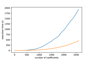
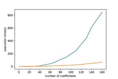
Figure 1: Execution time as a function of the number of computed coefficients for the stream solution of system (26) (left) and of system (23) (right). The orange (lower) curve is the recurrence relation (29) computed via Lemma 6.1 (authors’ Python code); the blue (upper) curve is the power series solution of (25) (Maple’s dsolve).

Remark 4 (Newton method).

In terms of complexity with respect to $k$ (number of computed coefficients), Newton iteration applied to formal power series [17, 29, 12, 8] does asymptotically better than the $O(k^{2})$ algorithm outlined above. In particular, [8, Th.3.12] shows that, under the same hypotheses of IFT, the first $k$ coefficients of the solution of a system of algebraic equation can be computed by Newton iteration in time $O(k\log k)$; on the downside, each iteration of Newton involves in general finding the solution of a $n\times n$ linear system.

7 Conclusion

In this paper, we have presented an implicit function theorem for the stream calculus, a powerful set of tools for reasoning on infinite sequences of elements from a given field. Our theorem is directly inspired from the analogous one from classical calculus. We have shown that the stream IFT has clear computational advantages over the classical one.

The present work can be extended in several directions. First, we would like to explore the relations of our work with methods proposed in the realm of numerical analysis for efficient generation of the Taylor coefficients of ODE’ solutions; see e.g. [11] and references therein. Second, we would like to go beyond the polynomial format, and allow for systems of equations $\mathcal{E}$ involving, for example, functions that are in turn defined via SDEs. Finally, we would like to extend the present results to the case of multivariate streams, that is consider a vector ${\boldsymbol{\mathrm{x}}}=(x_{1},...,x_{m})$ of independent variables, akin to the more general version of the classical IFT. Both extensions seem to pose nontrivial technical challenges.

Appendix A Three-coloured trees example: details

In order to generate the rational system (19), rather than explicitly determining the inverse of the Jacobian $\mathrel{\ooalign{$\nabla$\cr\hfil\scalebox{1.0}[1.0]{\rotatebox[origin={c}]{-70.0}{${}^{\setminus}$}\!}\hfil\cr}}_{{\boldsymbol{\mathrm{y}}}}\mathcal{E}$, it is practically convenient firstly to form the equivalent system (15) and then solve for ${\boldsymbol{\mathrm{y^{\prime}}}}$. To this purpose, we apply the syntactic stream derivative operator to the polynomial equations of system (26), obtaining:

$$\begin{cases}y_{1}^{\prime}-1-y_{2}^{\prime}y_{2}-y_{3}^{\prime}y_{3}-2y_{2}^{\prime}y_{3}&=0\\ y_{2}^{\prime}-y_{3}^{\prime}y_{3}-y_{1}^{\prime}y_{1}-2y_{3}^{\prime}y_{1}&=0\\ y_{3}^{\prime}-y_{1}^{\prime}y_{1}-y_{2}^{\prime}y_{2}-2y_{1}^{\prime}y_{2}&=0\,.\end{cases}$$ (30)

Then we note that (30) is a linear system in the variables ${\boldsymbol{\mathrm{y}}}^{\prime}=(y_{1}^{\prime},y_{2}^{\prime},y_{3}^{\prime})^{T}$ of the form $A{\boldsymbol{\mathrm{y^{\prime}}}}={\boldsymbol{\mathrm{b}}}$, where $A=(\mathrel{\ooalign{$\nabla$\cr\hfil\scalebox{1.0}[1.0]{\rotatebox[origin={c}]{-70.0}{${}^{\setminus}$}\!}\hfil\cr}}_{{\boldsymbol{\mathrm{y}}}}\mathcal{E})(0,{\boldsymbol{\mathrm{r}}}_{0},{\boldsymbol{\mathrm{y}}})=\left[\begin{smallmatrix}1&-y_{2}-2y_{3}&-y_{3}\\ -y_{1}&1&-y_{3}-2y_{1}\\ -y_{1}-2y_{2}&-y_{2}&1\end{smallmatrix}\right]$ and ${\boldsymbol{\mathrm{b}}}=-(\mathrel{\ooalign{$\nabla$\cr\hfil\scalebox{1.0}[1.0]{\rotatebox[origin={c}]{-70.0}{${}^{\setminus}$}\!}\hfil\cr}}_{x}\mathcal{E})(0,{\boldsymbol{\mathrm{y}}})^{T}=(1,0,0)^{T}$. Note that this is another way of writing system (15). Now, we solve $A{\boldsymbol{\mathrm{y^{\prime}}}}={\boldsymbol{\mathrm{b}}}$ for ${\boldsymbol{\mathrm{y^{\prime}}}}$. Denoting the determinant of $\mathrel{\ooalign{$\nabla$\cr\hfil\scalebox{1.0}[1.0]{\rotatebox[origin={c}]{-70.0}{${}^{\setminus}$}\!}\hfil\cr}}_{{\boldsymbol{\mathrm{y}}}}\mathcal{E}$ as

$$\Delta=2y_{1}^{2}y_{2}+4y_{1}^{2}y_{3}+4y_{1}y_{2}^{2}+10y_{1}y_{2}y_{3}+3y_{1}y_{2}+2y_{1}y_{3}^{2}+3y_{1}y_{3}+2y_{2}^{2}y_{3}+4y_{2}y_{3}^{2}+3y_{2}y_{3}-1$$

and taking into account the initial condition, we arrive at (19):

$$\begin{cases}y_{1}^{\prime}\,={\Delta^{-1}}\cdot(2y_{1}y_{2}+y_{2}y_{3}-1)&y_{1}(0)=0\\ y_{2}^{\prime}\,={\Delta^{-1}}\cdot(-2y_{1}^{2}-4y_{1}y_{2}-y_{1}y_{3}-y_{1}-2y_{2}y_{3})\;\;&y_{2}(0)=0\\ y_{3}^{\prime}\,={\Delta^{-1}}\cdot(-y_{1}y_{2}-y_{1}-2y_{2})&y_{3}(0)=0\,.\end{cases}$$ (31)

In order to convert the above rational SDE initial value problem to a polynomial one, we can apply Lemma 3.2. In practice, we replace $\Delta^{-1}$ with a new variable $w$, then we add the corresponding equation to system (31). In order to derive a SDE for the variable $w$, we recall that the multiplicative inverse $\sigma^{-1}$ of a stream $\sigma$ such that $\sigma(0)\neq 0$ satisfies the SDE and initial condition (3). In our case, starting from $w^{\prime}=w(0)\Delta^{\prime}w$, and calling $p_{1},p_{2},p_{3}$ the right-hand sides of the SDEs in (31), we get

$$\begin{cases}w^{\prime}&=w(0)\cdot(2y_{1}^{\prime}y_{1}y_{2}+4y_{1}^{\prime}y_{1}y_{3}+4y_{1}^{\prime}y_{2}^{2}+10y_{1}^{\prime}y_{2}y_{3}+3y_{1}^{\prime}y_{2}+2y_{1}^{\prime}y_{3}^{2}+3y_{1}^{\prime}+y_{3}\\ &\;\;\;\;+2y_{2}^{\prime}y_{2}y_{3}+4y_{2}^{\prime}y_{3}^{2}+3y_{2}^{\prime}y_{3})w\\ &=-(2p_{1}y_{1}y_{2}+4p_{1}y_{1}y_{3}+4p_{1}y_{2}^{2}+10p_{1}y_{2}y_{3}+3p_{1}y_{2}+2p_{1}y_{3}^{2}+3p_{1}+y_{3}\\ &\;\;\;\;+2p_{2}y_{2}y_{3}+4p_{2}y_{3}^{2}+3p_{2}y_{3})w\\ w(0)&=-1\end{cases}$$

where the initial condition $w(0)=-1$ is implied by $\Delta(0,{\boldsymbol{\mathrm{r}}}_{0})=-1$. Finally, expanding the $p_{i}$’s and putting everything together, we obtain the following polynomial system of SDEs and initial conditions:

$$\begin{cases}y_{1}^{\prime}\ =2wy_{1}y_{2}+wy_{2}y_{3}-w&y_{1}(0)=0\\ y_{2}^{\prime}\ =-2wy_{1}^{2}-4wy_{1}y_{2}-wy_{1}y_{3}-wy_{1}-2wy_{2}y_{3}&y_{2}(0)=0\\ y_{3}^{\prime}\ =-wy_{1}y_{2}-wy_{1}-2wy_{2}&y_{2}(0)=0\\ w^{\prime}\ =4w^{2}y_{1}^{2}y_{2}^{2}+4w^{2}y_{1}^{2}y_{2}y_{3}-8w^{2}y_{1}^{2}y_{3}^{2}-6w^{2}y_{1}^{2}y_{3}+8w^{2}y_{1}y_{2}^{3}+&w(0)=-1\\ \;\;\;\;\;\;\;\;\;\;14w^{2}y_{1}y_{2}^{2}y_{3}+6w^{2}y_{1}y_{2}^{2}-10w^{2}y_{1}y_{2}y_{3}^{2}-8w^{2}y_{1}y_{2}y_{3}-2w^{2}\\ \;\;\;\;\;\;\;\;\;\;y_{1}y_{2}-4w^{2}y_{1}y_{3}^{3}-7w^{2}y_{1}y_{3}^{2}-7w^{2}y_{1}y_{3}+4w^{2}y_{2}^{3}y_{3}+6w^{2}y_{2}^{2}\\ \;\;\;\;\;\;\;\;\;\;y_{3}^{2}+3w^{2}y_{2}^{2}y_{3}-4w^{2}y_{2}^{2}-6w^{2}y_{2}y_{3}^{3}-3w^{2}y_{2}y_{3}^{2}-10w^{2}y_{2}y_{3}-\\ \;\;\;\;\;\;\;\;\;\;3w^{2}y_{2}-2w^{2}y_{3}^{2}-3w^{2}y_{3}\,.\end{cases}$$ (32)

References

- [1] The on-line encyclopedia of integer sequences. https://oeis.org.
- [2] Henning Basold, Marcello M. Bonsangue, Helle Hvid Hansen, and Jan Rutten. (co)algebraic characterizations of signal flow graphs. In Horizons of the Mind. A Tribute to Prakash Panangaden - Essays Dedicated to Prakash Panangaden on the Occasion of His 60th Birthday, volume 8464 of LNCS, pages 124–145. Springer, 2014.
- [3] Filippo Bonchi, Pawel Sobocinski, and Fabio Zanasi. Full Abstraction for Signal Flow Graphs. Proc. of POPL, pages 515–526. ACM, 2015.
- [4] Filippo Bonchi, Pawel Sobocinski, and Fabio Zanasi. The Calculus of Signal Flow Diagrams I: Linear relations on streams. Inf. Comput., 252: 2–29. Elsevier, 2017.
- [5] Michele Boreale. Algebra, coalgebra, and minimization in polynomial differential equations. Log. Methods Comput. Sci., 15(1), 2019. doi:10.23638/LMCS-15(1:14)2019.
- [6] Michele Boreale. Complete algorithms for algebraic strongest postconditions and weakest preconditions in polynomial ODEs. Sci. Comput. Program., 193:102441, 2020. https://doi.org/10.1016/j.scico.2020.102441 doi:10.1016/j.scico.2020.102441.
- [7] M. Boreale, and D. Gorla. Algebra and Coalgebra of Stream Products. 32nd International Conference on Concurrency Theory (CONCUR 2021). Leibniz International Proceedings in Informatics (LIPIcs). 203: 19:1–19:17. Schloss Dagstuhl – Leibniz-Zentrum für Informatik, Dagstuhl, Germany, https://drops.dagstuhl.de/opus/volltexte/2021/14396, 2021.
- [8] Alin Bostan, Frédéric Chyzak, Marc Giusti, Romain Lebreton, Grégoire Lecerf, Bruno Salvy, Éric Schost. Algorithmes Efficaces en Calcul Formel. Palaiseau, France, 2018. URL: https://hal.archives-ouvertes.fr/AECF.
- [9] D. Cox, J. Little, and D. O’Shea. Ideals, Varieties, and Algorithms: An Introduction to Computational Algebraic Geometry and Commutative Algebra, 4/e. Undergraduate Texts in Mathematics. Springer, 2015.
- [10] Philippe Flajolet and Robert Sedgewick. Analytic combinatorics: functional equations, rational and algebraic functions. Research Report RR-4103, INRIA, 2001. URL: https://hal.inria.fr/inria-00072528.
- [11] Bengt Fornberg and J. A. C. Weideman. A Numerical Methodology for the Painlevé Equations. Journal of Computational Physics, 230(15):5957–73, 2011.
- [12] Aurel Galántai. The theory of Newton’s method. Journal of Computational and Applied Mathematics, 124(1-2):25–44, 2000.
- [13] Helle Hvid Hansen, Clemens Kupke, and Jan Rutten. Stream differential equations: Specification formats and solution methods. Log. Methods Comput. Sci., 13(1), 2017. doi:10.23638/LMCS-13(1:3)2017.
- [14] Bartek Klin. Bialgebras for structural operational semantics: An introduction. Theoretical Computer Science, 412(38):5043–5069, 2011. doi:https://doi.org/10.1016/j.tcs.2011.03.023.
- [15] Steven G. Krantz, Harold R. Parks. Implicit function theorem: history, theory, and applications. Undergraduate Texts in Mathematics. Springer, 2012.
- [16] W. Kuich and A. Salomaa. Semirings, Automata, Languages. Monographs in Theoretical Computer Science: An EATCS Series. Springer, 1986.
- [17] John D. Lipson. Newton’s method: A great algebraic algorithm. In Proc. of Symp. on Symbolic and Algebraic Computation. ACM, 1976.
- [18] Stefan Milius. A Sound and Complete Calculus for Finite Stream Circuits. In Proc. of LICS, pages 421–30. IEEE, 2010.
- [19] Dusko Pavlovic and M. Escardó. Calculus in coinductive form. In Proc. of LICS, pages 408–417. IEEE, 1998.
- [20] Damien Pous and Jurriaan Rot. Companions, Codensity, and Causality. In Proc. of FOSSACS, volume 10203 of LNCS, pages 106–123. Springer, 2017.
- [21] Walter Rudin. Principles of mathematical analysis. International series in pure and applied mathematics, McGraw-Hill, 1976.
- [22] Jan J. M. M. Rutten. Elements of Stream Calculus (An Extensive Exercise in Coinduction). Proc. of MFPS, volume 45 of ENTCS, pages 358–423. Elsevier, 2001.
- [23] Jan J. M. M. Rutten. Behavioural differential equations: a coinductive calculus of streams, automata, and power series. Theor. Comput. Sci., 308(1-3):1–53, 2003. doi:10.1016/S0304-3975(02)00895-2.
- [24] Jan J. M. M. Rutten. An Application of Stream Calculus to Signal Flow Graphs. Proc. of FMCO, volume 3188 in LNCS, pages 276–291. Springer, 2003.
- [25] Jan J. M. M. Rutten. A coinductive calculus of streams. Math. Struct. Comput. Sci., 15(1):93–147, 2005. doi:10.1017/S0960129504004517.
- [26] Jan J. M. M. Rutten. A tutorial on coinductive stream calculus and signal flow graphs. Theor. Comput. Sci., 343(3):443–481. Elsevier, 2005.
- [27] Davide Sangiorgi. Introduction to Bisimulation and Coinduction. CUP, 2011.
- [28] Giovanni M. Scarpello, and Daniele Ritelli. A Historical Outline of the Theorem of Implicit Functions. Divulgaciones Matematicas, 10(2): 171–180, 2022.
- [29] Arnold Schönhage. The fundamental theorem of algebra in terms of computational complexity. Preliminary Report. Mathematisches Institut der Universität Tübingen, 1982.
- [30] Richard P. Stanley. Enumerative Combinatorics, Vol. 1, 2nd edition. Cambridge Studies in Advanced Mathematics, 2012.
- [31] Joost Winter. Coalgebraic Characterizations of Automata-Theoretic Classes. PhD thesis, Radboud Universiteit Nijmegen, 2014.