Doubly Regularized Entropic Wasserstein Barycenters

Abstract

We study a general formulation of regularized Wasserstein barycenters that enjoys favorable regularity, approximation, stability and (grid-free) optimization properties. This barycenter is defined as the unique probability measure that minimizes the sum of entropic optimal transport (EOT) costs with respect to a family of given probability measures, plus an entropy term. We denote it $(\lambda,\tau)$-barycenter, where $\lambda$ is the inner regularization strength and $\tau$ the outer one. This formulation recovers several previously proposed EOT barycenters for various choices of $\lambda,\tau\geq 0$ and generalizes them. First, in spite of – and in fact owing to – being doubly regularized, we show that our formulation is debiased for $\tau=\lambda/2$: the suboptimality in the (unregularized) Wasserstein barycenter objective is, for smooth densities, of the order of the strength $\lambda^{2}$ of entropic regularization, instead of $\max\{\lambda,\tau\}$ in general. We discuss this phenomenon for isotropic Gaussians where all $(\lambda,\tau)$-barycenters have closed form. Second, we show that for $\lambda,\tau>0$, the barycenter has a smooth density and is strongly stable under perturbation of the marginals. In particular, it can be estimated efficiently: given $n$ samples from each of the probability measures, it converges in relative entropy to the population barycenter at a rate $n^{-1/2}$. And finally, this formulation lends itself naturally to a grid-free optimization algorithm: we propose a simple noisy particle gradient descent which, in the mean-field limit, converges globally at an exponential rate to the barycenter.

1 Introduction

Given a family of probability measures, its Wasserstein barycenter is a probability measure that summarizes it in a geometrically faithful way. This object, first studied in [AC11], has found numerous applications in statistics [BBR06, BLL15, BJGR19], image processing [RPDB11], computer graphics [Sol+15] and Bayesian inference [SLD18, BFRT22] (see [PC19, Chap. 9.2] or [PZ20] for introductions to this topic). While it is arguably one of the most natural notion of barycenters for probability measures, the Wasserstein barycenter is unfortunately difficult to estimate and compute in large-scale applications.

To overcome these limitations and following the idea of entropic regularization of optimal transport, a.k.a the Schrödinger bridge problem [Sch32, Wil69, ES90, KY94, Léo12, Cut13], various formulations of entropy-regularized Wasserstein barycenters have been proposed and studied in the literature (discussed below). In these works, entropic regularization is incorporated in two different ways, which we refer to as inner and outer regularizations, and with various reference measures. It is not clear a priori how these formulations relate to each other, and whether a particular one stands out for its mathematical or practical properties.

In this paper, we aim at clarifying and generalizing the picture by considering both inner and outer regularizations at the same time. We prove that this formulation combines favorable analytical, approximation, stability and optimization properties, which are all enabled by the positive interaction between those two entropic regularizations.

1.1 Entropic optimal transport (EOT)

Let $\mathcal{X}$ be a compact and convex subset of $\mathbb{R}^{d}$ with nonempty interior and let $c\in\mathcal{C}^{p}(\mathcal{X}\times\mathcal{X})$ for some $p\geq 2$. For two probability measures $\mu,\nu\in\mathcal{P}(\mathcal{X})$, let $\Pi(\mu,\nu)$ be the set of transport plans between $\mu$ and $\nu$ and define the Entropic Optimal Transport (EOT) cost as

$$T_{\lambda}(\mu,\nu)\coloneqq\min_{\gamma\in\Pi(\mu,\nu)}\int_{\mathcal{X}\times\mathcal{X}}c(x,y)\mathrm{d}\gamma(x,y)+\lambda H(\gamma|\mu\otimes\nu)$$ (1)

where $\lambda\geq 0$ is the regularization strength and $H(\mu|\nu)=\int\log\big{(}\frac{\mathrm{d}\mu}{\mathrm{d}\nu}\big{)}\mathrm{d}\mu$ if $\mu\ll\nu$ and $+\infty$ otherwise, is the relative entropy. Notice the choice of reference measure $\mu\otimes\nu$ for the regularization term in (1), which is important for our exposition, see Section 3.3. With this choice, $T_{\lambda}$ is always finite, even for discrete measures (indeed, $\gamma=\mu\otimes\nu$ is a feasible point). Setting the regularization $\lambda$ to $0$, we recover the standard optimal transport problem, and the $L^{2}$-Wasserstein distance $W_{2}$ is defined as $W_{2}\coloneqq\sqrt{2T_{0}}$ when $c(x,y)=\frac{1}{2}\|y-x\|^{2}_{2}$.

1.2 Doubly Regularized EOT Barycenter

Given a family of $K$ probability measures $(\nu_{1},\dots,\nu_{K})\in\mathcal{P}(\mathcal{X})^{K}$ and $K$ weights $(w_{1},\dots,w_{K})\in\mathbb{R}_{+}^{K}$ summing to $1$, we define the EOT barycenter functional $G_{\lambda}:\mathcal{P}(\mathcal{X})\to\mathbb{R}$ as

$$G_{\lambda}(\mu)\coloneqq\sum_{k=1}^{K}w_{k}T_{\lambda}(\mu,\nu_{k}).$$ (2)

We also denote by $H$ is the (negative) differential entropy

$$H(\mu)\coloneqq\int_{\mathcal{X}}\log\Big{(}\frac{\mathrm{d}\mu}{\mathrm{d}x}\Big{)}\mathrm{d}\mu(x)$$ (3)

if $\mu$ is absolutely continuous and $+\infty$ otherwise. Our main object of study is the following doubly regularized EOT barycenter.

As shown in Section 3.3, for absolutely continuous measures, $(\lambda,\tau)$-barycenters can also be interpreted as EOT barycenters with only inner regularization, but with a different reference measure $\sigma_{\mathrm{ref}}$ (replacing $\mu\otimes\nu$ in (1)):

$$\sigma_{\mathrm{ref}}=\Big{[}\Big{(}\frac{\mathrm{d}\mu}{\mathrm{d}x}\Big{)}^{\alpha}\mathrm{d}x\Big{]}\otimes\Big{[}\Big{(}\frac{\mathrm{d}\nu}{\mathrm{d}y}\Big{)}^{\alpha}\mathrm{d}y\Big{]} \alpha\coloneqq 1-\tau/\lambda<1.$$ where (5)

This in particular includes the case $\alpha=0$, that is $\sigma_{\mathrm{ref}}=\mathrm{d}x\otimes\mathrm{d}y$ (for $\tau=\lambda$) which is the historical formulation of EOT with Lebesgue as a reference measure known as the Schrödinger bridge problem. It follows that $(\lambda,\lambda)$-barycenters have implicitly been considered in many works [CD14, CP18, BCP19a] (see, e.g. the reference book [PC19, Chap. 9.2]). As we will see, interpreting those barycenters as doubly-regularized lead to a simpler and stronger analysis of their properties. We will also see that $(\lambda,\nicefrac{{\lambda}}{{2}})$-barycenters (corresponding to $\alpha=\nicefrac{{1}}{{2}}$) are in fact superior in terms of approximation of the $(0,0)$-barycenter. We mention that the general formulation of $(\lambda,\tau)$-barycenters in Def. 1.1 already appears in [BBB20] where it is motivated by computational purposes and the analysis requires the constraint $\lambda<\tau$.

1.3 Relation to barycenters in the literature

Various notions of barycenters for probability measures based on (entropy-regularized) optimal transport can be found in the literature. Most of them can be seen as $(\lambda,\tau)$-barycenters for particular choices of $\lambda$ and $\tau$ (see Table 1 for a summary).

1. Unregularized OT barycenters. They are the minimizers $\mu_{0,0}^{*}$ of $G_{0}$ in $\mathcal{P}(\mathcal{X})$, they were first studied in [AC11] and correspond to $(0,0)$-barycenters in Def. 1.1. Under our assumptions, minimizers always exist but might not be unique. Uniqueness holds for instance in the case $c(x,y)\propto\|y-x\|_{2}^{2}$ and if at least one of the $\nu_{k}$ vanishes on small-sets (a condition weaker than absolute continuity) [AC11].

2. Inner-regularized barycenters. They are defined as the minimizers of $G_{\lambda}$ and correspond to $(\lambda,0)$-barycenters. Uniqueness of this barycenter is not always granted as $G_{\lambda}$ is not strictly convex (think of $c$ the constant cost for which any $\mu\in\mathcal{P}(\mathcal{X})$ is a barycenter). Compared to $\mu_{0,0}^{*}$, here the regularization typically induces a shrinking bias. In particular, the barycenter of Gaussians can be a Dirac mass when their covariances is small compared to $\lambda$ [JCG20] (see also Section 3.2). To understand this, one may verify that for the square-distance cost, the minimizer of $T_{\lambda}(\cdot,\mu)$ is $\mu$ itself only when $\lambda=0$ (or $\mu$ is a Dirac mass), and otherwise, it is a deconvolution of $\mu$ [RW18].

3. To correct this fact and recover a distance-like quantity, the Sinkhorn divergence $S_{\lambda}(\mu,\nu)\coloneqq T_{\lambda}(\mu,\nu)-\frac{1}{2}T_{\lambda}(\mu,\mu)-\frac{1}{2}T_{\lambda}(\nu,\nu)$ as been introduced [RGC17]. It is indeed a positive definite quantity as long as $e^{-c/\lambda}$ is a positive definite universal kernel [Fey+19], which is the case e.g. for $c(x,y)\propto\|x-y\|^{2}_{2}$. This suggests to consider Sinkhorn divergence barycenters [JCG20], i.e. the minimizers of

   $$\mu\mapsto\sum_{k=1}^{K}w_{k}S_{\lambda}(\mu,\nu)=G_{\lambda}(\mu)-\tfrac{1}{2}T_{\lambda}(\mu,\mu)+C$$

   where $C\in\mathbb{R}$ does not depend on $\mu$. The self-EOT term effectively “debiases” the barycenter: this is shown for Gaussians in [JCG20], and for general smooth measures in Section 3. However, little else is known about this barycenter (regarding uniqueness, stability or regularity). This formulation is not covered by Def. 1.1.

4. Schrödinger barycenters. In most works (e.g. [CD14, CP18, BCP19a]), inner-regularized barycenters are in fact considered with Lebesgue as a reference measure in (1) instead of $\mu\otimes\nu$. As discussed in the previous paragraph, they correspond to $(\lambda,\lambda)$-barycenters. This regularization leads to a blurring bias.

5. Outer-regularized barycenters. These are the minimizers of $G_{0}+\tau H$, studied in [BCP19, CEK21], which correspond to $(0,\tau)$-barycenters in Def. 1.1. This barycenter has interesting regularity properties: for instance [CEK21] show bounds on the $L^{\infty}$ norm, moments and regularity of the barycenter (which are not known for the inner-regularized barycenters). This regularization induces a blurring bias as well.

As can be seen, all the previously proposed OT-like barycenters – except the Sinkhorn divergence barycenter – appear to be $(\lambda,\tau)$-barycenters, with various formulations corresponding to different subsets of the $(\lambda,\tau)$ plane. In our analysis, we will often restrict ourselves to $\lambda,\tau>0$ for convenience.

Barycenter	Objective	Approximation	Notation
Un-regularized	$G_{0}$	exact	$\mu_{0,0}^{*}$
Inner-regularized	$G_{\lambda}$	shrinked	$\mu_{\lambda,0}^{*}$
Sinkhorn divergence	$G_{\lambda}-\frac{1}{2}T_{\lambda}(\cdot,\cdot)$	debiaised	$\mu_{\lambda,\mathrm{div}}^{*}$
Schrödinger	$G_{\lambda}+\lambda H$	blurred	$\mu^{*}_{\lambda,\lambda}$
Outer-regularized	$G_{0}+\tau H$	blurred	$\mu_{0,\tau}^{*}$
Doubly-regularized	$G_{\lambda}+\tau H$	debiased for $\tau=\frac{\lambda}{2}$	$\mu_{\lambda,\tau}^{*}$

Table 1: List of the various formulations of OT-like barycenters. The third column is an informal description of the bias from $\mu_{0,0}^{*}$ when the marginals $\nu_{k}$ are smooth densities, see Section 3 for precise statements.

1.4 Contributions

Our contributions are the following:

• in Section 2, we discuss basic variational properties of $(\lambda,\tau)$-barycenters. In particular, we prove that for $\lambda,\tau>0$, they have a smooth log-density (Thm. 2.5) and we derive a dual formulation (Prop. 2.6).

• in Section 3, we study the approximation error of $(\lambda,\tau)$-barycenter with respect to the unregularized Wasserstein barycenter for the square-distance cost. We prove that for smooth marginals $\nu_{1},\dots,\nu_{K}$, the suboptimality of $(\lambda,\nicefrac{{\lambda}}{{2}})$-barycenters in the Wasserstein barycenter functional $G_{0}$ is of the order $\lambda^{2}$ and that the same holds for Sinkhorn divergence barycenters (Thm. 3.2). We also compute and discuss the closed form of $(\lambda,\tau)$-barycenters between isotropic Gaussians (Prop. 3.4).

• In Section 4, we give stability bounds for $(\lambda,\tau)$-barycenters (Thm. 4.1). A consequence of these stability bounds is that they can be estimated in relative entropy given $n$ independent samples from each $\nu_{k}$ with an expected error in $O(\tau^{-1}(1+\lambda^{-d/2})n^{-1/2})$.

• To compute this barycenter, we introduce in Section 5 a grid-free numerical method: Noisy Particle Gradient Descent (NPGD). We prove the well-posedness and exponential convergence to the global minimizer (Thm. 5.1) of this optimization dynamics in the mean-field limit, i.e. when the number of particles grows to infinity.

• Numerical results are presented in Section 6. There we give examples of $(\lambda,\tau)$-barycenters on a simple 1D problem solved via convex optimization and we illustrate the global convergence of the grid-free method NPGD on an example where $G_{0}$ has a spurious minimizer.

Blanket assumptions

Throughout $\mathcal{X}\subset\mathbb{R}^{d}$ is a compact convex set with nonempty interior and $c\in\mathcal{C}^{p}(\mathcal{X}\times\mathcal{X})$ for some $p\geq 2$.

2 Well-posedness and regularity

This section contains basic mathematical results about $(\lambda,\tau)$-barycenters and the optimization problem defining them (Def. 1.1).

2.1 Preliminaries: regularity of EOT

Let us begin with some useful facts about EOT. The problem (1) that defines $T_{\lambda}$ has a unique solution $\gamma^{*}\in\mathcal{P}(\mathcal{X}\times\mathcal{X})$ and admits the dual formulation

$$T_{\lambda}(\mu,\nu)=\max_{\phi\in L^{1}(\mu),\psi\in L^{1}(\nu)}\int\phi\mathrm{d}\mu+\int\psi\mathrm{d}\nu+\lambda\Big{(}1-\int e^{(\phi(x)-\psi(y)-c(x,y))/\lambda}\mathrm{d}\mu(x)\mathrm{d}\nu(y)\Big{)}.$$ (6)

This dual problem has a solution $(\phi^{*},\psi^{*})$ which is unique in $L^{1}(\mu)\times L^{1}(\nu)$ up to the transformation $(\phi^{*}+c,\psi^{*}-c)$ for $c\in\mathbb{R}$. At optimality, we have $T_{\lambda}(\mu,\nu)=\int\phi^{*}\mathrm{d}\mu+\int\psi^{*}\mathrm{d}\nu$ and the primal-dual relation $\gamma(\mathrm{d}x,\mathrm{d}y)=e^{(\phi(x)+\psi(y)-c(x,y))/\lambda}\mu(\mathrm{d}x)\nu(\mathrm{d}y).$ Moreover, the potentials satisfy for $\mu\otimes\nu$ almost every $(x,y)$, the optimality condition

$$\left\{\begin{aligned} \phi^{*}(x)&=-\lambda\log\Big{(}\int e^{(\psi^{*}(y)-c(x,y))/\lambda}\mathrm{d}\nu(y)\Big{)}\\ \psi^{*}(y)&=-\lambda\log\Big{(}\int e^{(\phi^{*}(x)-c(x,y))/\lambda}\mathrm{d}\mu(x)\Big{)}\end{aligned}\right..$$ (7)

These equations can be used to extend $\phi^{*}$ and $\psi^{*}$ as continuous functions (in fact of class $\mathcal{C}^{p}$ when $c\in\mathcal{C}^{p}$) over $\mathcal{X}$, which satisfy these equations everywhere [GCBCP19].

Definition 2.1 (Schrödinger potentials).

The pair of functions $(\phi,\psi)\in\mathcal{C}^{p}(\mathcal{X})\times\mathcal{C}^{p}(\mathcal{X})$ which satisfies the Schrödinger system Eq. (7) for all $(x,y)\in\mathcal{X}^{2}$ is called the Schrödinger potentials. This pair is unique up to the transformation $(\phi^{*}+c,\psi^{*}-c)$ for $c\in\mathbb{R}$ (the choice of which does not matter in what follows).

This particular choice of potentials among all those that satisfy Eq. (7) $\mu\otimes\nu$-almost everywhere is justified by the following result.

Proposition 2.2 (First-variation of entropic optimal transport).

Fix $\nu\in\mathcal{P}(\mathcal{X})$ and for $\mu\in\mathcal{P}(\mathcal{X})$ let $(\phi[\mu],\psi[\mu])$ be the Schrödinger potentials associated to the pair $(\mu,\nu)$. Then:

• The map $\mu\mapsto\phi[\mu]$ (as well as the map $\mu\mapsto\psi[\mu]$) satisfies the following Lipschitz continuity property: there exists $L>0$ such that

  $$\|\phi[\mu]-\phi[\mu^{\prime}]\|_{\tilde{\mathcal{C}}^{p-1}(\mathcal{X})}\leq L\,W_{2}(\mu,\mu^{\prime}),\quad\forall\mu,\mu^{\prime}\in\mathcal{P}(\mathcal{X}).$$

  where $\|\cdot\|_{\tilde{\mathcal{C}}^{p-1}(\mathcal{X})}$ denotes the maximum supremum norm of all partial derivatives up to order ${p-1}$ quotiented by the invariance by addition of a constant (as in Def. 2.1).

• the function $\mu\mapsto T_{\lambda}(\mu,\nu)$ is convex, weakly continuous, and admits $\phi_{\mu}$ as first-variation, i.e.

  $$\forall\mu,\tilde{\mu}\in\mathcal{P}(\mathcal{X}),\;\lim_{\epsilon\,\downarrow\,0}\frac{1}{\epsilon}\Big{(}T_{\lambda}((1-\epsilon)\mu+\epsilon\tilde{\mu},\nu)-T_{\lambda}(\mu,\nu)\Big{)}=\int_{\mathcal{X}}\phi[\mu](x)\mathrm{d}(\tilde{\mu}-\mu)(x).$$ (8)

• For any $p^{\prime}\in\{0,\dots,p\}$ there exists $C_{p^{\prime}}>0$ independent of $\mu,\nu$ and $\lambda$ such that

  $$\|\phi[\mu]\|_{\tilde{\mathcal{C}}^{p^{\prime}}}\leq C_{p^{\prime}}\lambda^{\min\{0,1-p^{\prime}\}}.$$

Proof.

The first claim is technical and is proved in [CCM22] via the implicit function theorem on the Schrödinger system (7). The convexity of $T_{\lambda}(\cdot,\nu)$ is clear by Eq. (6) which expresses this function as a supremum of (weakly continuous) affine forms. To prove that $\phi[\mu]$ is the first-variation as in [Fey+19], let $\mu_{\epsilon}\coloneqq(1-\epsilon)\mu+\epsilon\tilde{\mu}$. Using the fact that $\phi[\mu]$ (resp. $\phi[\mu_{\epsilon}]$) is a subgradient of $T_{\lambda}(\cdot,\nu)$ at $\mu$ (resp. at $\mu_{\epsilon}$), we have

$$\int\phi[\mu]\mathrm{d}(\tilde{\mu}-\mu)\leq\frac{1}{\epsilon}\Big{(}T_{\lambda}(\mu_{\epsilon},\nu)-T_{\lambda}(\mu,\nu)\Big{)}\leq\int\phi[\mu_{\epsilon}]\mathrm{d}(\tilde{\mu}-\mu).$$

The point (ii) follows from the weak continuity of $\mu\mapsto\phi[\mu]$, a consequence of (i). Finally (iii) is proved in [GCBCP19] where it is obtained by differentiating $p^{\prime}$ times Eq. (7) and applying Faà di Bruno’s formula. ∎

Let us mention that the Lipschitz constant $L$ in (i) may depend exponentially on the oscillation of $c/\lambda$, namely $(\sup c-\inf c)/\lambda$.

2.2 Regularity of $(\lambda,\tau)$-barycenters

We first gather useful regularity properties of $G_{\lambda}$, which are direct consequences of Prop. 2.2.

Proposition 2.3 (Regularity of $G_{\lambda}$).

For any $(\nu_{k})_{k=1}^{K}\in\mathcal{P}(\mathcal{X})^{K}$, the function $G_{\lambda}\colon\mathcal{P}(\mathcal{X})\to\mathbb{R}_{+}$ defined in Eq. (2) is convex, weakly continuous, and for any $\mu\in\mathcal{P}(\mathcal{X})$ it admits a first-variation

$$V[\mu]\coloneqq\sum_{k=1}^{K}w_{k}\phi_{k}[\mu]$$ (9)

where $\phi_{k}[\mu]\in\mathcal{C}^{p}(\mathcal{X})$ is the Schrödinger potential from $\mu$ to $\nu_{k}$. The map $\mu\mapsto\nabla V[\mu]$ is Lipschitz continuous in the sense that there exists $L>0$ such that

$$\|V[\mu]-V[\mu^{\prime}]\|_{\tilde{\mathcal{C}}^{p-1}}\leq L\,W_{2}(\mu,\mu^{\prime}),\qquad\forall\mu,\mu^{\prime}\in\mathcal{P}(\mathcal{X}).$$

We moreover have that for $p^{\prime}\leq p$, there exists $C_{p^{\prime}}>0$ independent of $\lambda>0$, $(w_{k})_{k}$ and $(\nu_{k})_{k}$ such that $\|V[\mu]\|_{\tilde{\mathcal{C}}^{p^{\prime}}}\leq C_{p^{\prime}}\lambda^{\min\{0,1-p^{\prime}\}}$.

Conveniently, the objective is also strongly convex.

Proposition 2.4 (Strong convexity of $F_{\tau,\lambda}$).

For $\lambda\geq 0$, the objective $F_{\lambda,\tau}=G_{\lambda}+\tau H$ is $\tau$-strongly convex on $\mathcal{P}(\mathcal{X})$ for the total variation norm.

Proof.

It is well known that $\mu\mapsto H(\mu)$ is $1$-strongly convex over $\mathcal{P}(\mathcal{X})$ for the total variation norm, see e.g. [Yu13, Cor. 1]. Since $G_{\lambda}$ is convex, the result follows. ∎

Strong convexity in $\ell^{2}$-norm on a discrete space $\mathcal{X}$ (which follows from Prop. 2.4 since then the total variation norm is the $\ell^{1}$ norm, and $\|\cdot\|_{\ell^{2}}\leq\|\cdot\|_{\ell^{1}}$) was already shown for the $(\lambda,\lambda)$-barycenter functional in [BCP19, Thm. 3.4] with a technical proof specific to that case. The equivalent formulation as a doubly-regularized problem makes this property immediate.

As a consequence of all these regularity results, we now show that $(\lambda,\tau)$-barycenters can be written as a smooth Gibbs density.

Proof.

The functional $G_{\lambda}$ is weakly continuous and $H$ is weakly lower-semicontinuous [San15, Sec. 7.1.2] so $F_{\lambda}$ is weakly lower-semicontinuous. It is not identically $+\infty$ since the normalized Lebesgue measure on $\mathcal{X}$ is a feasible point. Since $\mathcal{P}(\mathcal{X})$ is weakly compact, the direct method of the calculus of variations tells us that there exists at least one minimizer $\mu^{*}_{\lambda,\tau}$. Moreover $F_{\lambda,\tau}$ is strictly convex (Prop. 2.4), so the minimizer is unique and since $H(\mu^{*}_{\lambda})<\infty$ this measure is absolutely continuous. The first order optimality condition states that there exists $C\in\mathbb{R}$ such that

$$\sum_{k=1}^{K}w_{k}\phi_{k}[\mu^{*}_{\lambda,\tau}](x)+\tau\log\Big{(}\frac{\mathrm{d}\mu^{*}_{\lambda,\tau}}{\mathrm{d}x}(x)\Big{)}=C,\quad\text{for $\mu^{*}_{\lambda,\tau}$-almost every $x$}.$$ (11)

It remains to observe that $\mu^{*}_{\lambda,\tau}$ must have full support on $\mathcal{X}$ (this is because of the infinite negative slope of $s\log(s)$ at $0$, see e.g. [San15, Prop. 8.7] for details in a similar context) to obtain the formula for the minimizer. ∎

Interestingly, the minimizer of $F_{\lambda,\tau}$ for $\tau>0$ has always full support in $\mathcal{X}$ even when none of the marginals $\nu_{1},\dots,\nu_{K}$ have. This property is not satisfied when $\tau=0$ or for the Sinkhorn Divergence barycenter (see Section 3.2 for the case of point mass marginals).

Relation to prior works

To the best of our knowledge, little is known on the regularity of the regularity of $(0,0)$-barycenters beyond absolute continuity under the condition that at least one $\nu_{k}$ is absolutely continuous [AC11],[KP17, Thm. 5.1]. The only other regularity result we are aware of concerns $(0,\tau)$-barycenters and the quadratic cost: [CEK21] show a Fisher Information bound on $\mu^{*}_{0,\tau}$ (their Lem. 4.1) that imply Lipschitz regularity in the compact case : this is consistent with the $\lambda\to 0$ limit of Thm. 2.5. They additionally show (their Prop. 5.2) that $\mu^{*}_{0,\tau}$ gains two degree of regularity compared to the densities $\nu_{k}$. With $\lambda,\tau>0$, we see that the $(\lambda,\tau)$-barycenters are as regular as the cost function, no matter the marginals.

2.3 Dual formulations

There are several ways to derive a dual formulation for (4). Let us detail one of them which stands out as an elegant composition of two soft-max (log-sum-exp) functions – which is the dual consequence of the double regularization. It can be used to compute $(\lambda,\tau)$-barycenters in practice (Section 6).

Proposition 2.6.

For $\lambda,\tau>0$, one has the dual formulation

$$\min_{\mu\in\mathcal{P}(\mathcal{X})}F_{\lambda,\tau}(\mu)=\max_{{\boldsymbol{\psi}}\in\mathcal{C}(\mathcal{X})^{K}}E({\boldsymbol{\psi}})$$ (12)

where $$E({\boldsymbol{\psi}})$$ is defined as

$$\sum_{k=1}^{K}w_{k}\int_{\mathcal{X}}\psi_{k}\mathrm{d}\nu_{k}-\tau\log\left\{\int_{\mathcal{X}}\exp\left[\frac{\lambda}{\tau}\sum_{k=1}^{K}w_{k}\log\int_{\mathcal{X}}\exp\Big{(}\frac{\psi_{k}(y)-c(x,y)}{\lambda}\Big{)}\mathrm{d}\nu_{k}(y)\right]\mathrm{d}x\right\}.$$ (13)

The function $E$ is concave, $1$-Lipschitz continuous and $\min\{\lambda,\tau\}^{-1}$-smooth for the seminorm ${\boldsymbol{\psi}}\mapsto\sum w_{k}\|\psi_{k}\|_{\mathrm{osc}}$ where $\|\psi\|_{\mathrm{osc}}=\sup_{y}\psi(y)-\inf_{y}\psi(y)$. It admits a maximizer with semi-norm smaller than $\|c\|_{\mathrm{osc}}$ (which is unique up to shifting each $\psi_{k}$ by constants). Moreover, the barycenter $\mu^{*}_{\lambda,\tau}$ is a Gibbs distribution associated the solution of the dual problem (see (16)).

Proof.

We start from the dual formulation (6) of $T_{\lambda}(\mu,\nu)$. Maximizing over $\phi$ gives $\phi=\phi_{\psi}$ $\nu$-a.e. with

$$\phi_{\psi}(x)=-\lambda\log\Big{(}\int e^{(\psi(y)-c(x,y))/\lambda}\mathrm{d}\nu(y)\Big{)}$$ (14)

(this is half of the Schrödinger system (7)). The so-called “semi-dual” formulation of EOT follows

$$T_{\lambda}(\mu,\nu)=\max_{\psi\in\mathcal{C}(\mathcal{X})}\int\psi\mathrm{d}\nu+\int\phi_{\psi}\mathrm{d}\nu.$$ (15)

We can thus rewrite the objective of the barycenter as

$$\min_{\mu\in\mathcal{P}(\mathcal{X})}\max_{{\boldsymbol{\psi}}\in\mathcal{C}(\mathcal{X})^{K}}\sum_{k=1}^{K}w_{k}\int\psi_{k}\mathrm{d}\nu_{k}+\int\Big{(}\sum_{k=1}^{K}w_{k}\phi_{\psi_{k}}\Big{)}\mathrm{d}\mu+\tau H(\mu)$$

where $\phi_{\psi_{k}}$ is defined as in (14) but with $\nu_{k}$ in place of $\nu$. By Sion’s minimax theorem (using in particular that $\mathcal{P}(\mathcal{X})$ is weakly compact and that the semi-dual objective (15) is continuous for the sup-norm), we can exchange the order of min and max. Maximizing in $\mu\in\mathcal{P}(\mathcal{X})$ gives

$$\mu=\mu_{\boldsymbol{\psi}}=\exp\left((\chi_{\boldsymbol{\psi}}-V_{\boldsymbol{\psi}})/\tau\right) V_{\boldsymbol{\psi}}\coloneqq\sum_{k=1}^{K}w_{k}\phi_{\psi_{k}} \quad\chi_{\boldsymbol{\psi}}=-\tau\log\int e^{-V_{\boldsymbol{\psi}}/\tau}\mathrm{d}x$$ with and (16)

and the objective becomes $\max_{(\psi_{k})_{k}\in\mathcal{C}(\mathcal{X})^{K}}\sum_{k=1}^{K}w_{k}\int\psi_{k}\mathrm{d}\nu_{k}+\chi_{\boldsymbol{\psi}}.$

The other claims follow mostly from the general properties of the log-sum-exp operator $f\mapsto\mathrm{LSE}(f):x\mapsto\alpha\log\int e^{f(x,y)/\alpha}\mathrm{d}\nu(y)$ for $\alpha>0$ and $\nu$ a nonnegative measure, which is such that :

• if $f(\cdot,y)$ is convex for $\nu$-a.e $y$ then $\mathrm{LSE}(f)$ is convex in $x$ [BV04, Ex. 3.14];

• $\mathrm{LSE}$ is $1$-Lipschitz continuous and $1/\alpha$-smooth for the sup-norm, which can be seen from the expression of the first and second order differential:

  $$D\mathrm{LSE}[f](\delta f)=x\mapsto\mathbf{E}_{Y_{x}}[\delta f(x,Y_{x})] D^{2}\mathrm{LSE}[f](\delta f,\delta f)=x\mapsto\frac{1}{\alpha}\mathbf{Var}_{Y_{x}}[\delta f(x,Y_{x})]$$

  where $\mathbf{E}_{Y_{x}}$ (resp. $\mathbf{Var}_{Y_{x}}$) denote the expectation (resp. centered variance) under $Y_{x}$ distributed according to the probability measure proportional to $e^{f(x,y)/\alpha}\nu(\mathrm{d}y)$.

Let us apply these properties in the context of $E$. The second term of (12) is concave (as minus the composition of: an affine function, by a LSE, by a sum with nonnegative weights, by a LSE). It is also $1$-Lipschitz continuous, as a composition of $1$-Lipschitz continuous functions and its differential is given by

$$DE[{\boldsymbol{\psi}}](\delta\psi_{k})=w_{k}\int\delta\psi_{k}\mathrm{d}\nu_{k}-w_{k}\int\delta\psi_{k}(y)e^{(\phi_{\psi_{k}}(x)+\psi_{k}(y)-c(x,y))/\lambda+(\chi_{\boldsymbol{\psi}}(x)-V_{\boldsymbol{\psi}}(x))/\tau}\mathrm{d}x\mathrm{d}\nu_{k}(y)$$

Note that the second integral is the integral of $\delta\psi_{k}$ against a probability measure $\gamma_{\psi_{k}}(\mathrm{d}x,\mathrm{d}y)\in\Pi(\mu_{\boldsymbol{\psi}},\nu_{k})$ which can be disintegrated as $\gamma_{\psi_{k}}(\mathrm{d}y|x)\mu_{\boldsymbol{\psi}}(\mathrm{d}x)$. Differentiating once more, we obtain

$$D^{2}E[{\boldsymbol{\psi}}](\delta\psi,\delta\psi)=-\frac{1}{\tau}\mathbf{Var}_{x\sim\mu_{\boldsymbol{\psi}}}\Big{[}\sum_{k=1}^{K}w_{k}\mathbf{E}_{\gamma_{\psi_{k}}(\cdot|x)}[\delta\psi_{k}]\Big{]}-\frac{1}{\lambda}\mathbf{E}_{x\sim\mu_{\boldsymbol{\psi}}}\Big{[}\sum_{k=1}^{K}w_{k}\mathbf{Var}_{\gamma_{\psi_{k}}(\cdot|x)}(\delta\psi_{k})\Big{]}.$$

It follows by the law of total variance that

$$-\frac{1}{\max\{\tau,\lambda\}}\mathbf{Var}\Big{[}\sum_{k=1}^{K}w_{k}\delta\psi_{k}(y_{k})\Big{]}\geq D^{2}E[{\boldsymbol{\psi}}](\delta\psi,\delta\psi)\geq-\frac{1}{\min\{\tau,\lambda\}}\mathbf{Var}\Big{[}\sum_{k=1}^{K}w_{k}\delta\psi_{k}(y_{k})\Big{]}$$

where the variance is under $(x,y_{1},\dots,y_{k})$ such that $(x,y_{k})\sim\gamma_{\psi_{k}}$. This shows that $E$ is $\frac{1}{\min\{\tau,\lambda\}}$-smooth for the norm ${\boldsymbol{\psi}}\mapsto\sum w_{k}\|\psi_{k}\|_{\mathrm{osc}}$ and the uniqueness of the dual solution up to constant shifts. The existence of a maximizer can be obtained by taking the Schrödinger potentials associated to the minimizers (11) which satisfy the optimality conditions and the upper-bound on its semi-norm follows from the Schrödinger system (7). ∎

Dual formulation for $\lambda=\tau$

For the sake of completeness, let us mention that when $\tau=\lambda$, another useful dual formulation becomes available. Indeed, the problem then writes

$$\min_{\mu\in\mathcal{P}(\mathcal{X})}\max_{{\boldsymbol{\phi}},{\boldsymbol{\psi}}}\sum_{k}w_{k}\int\varphi_{k}\mathrm{d}\mu+\int\psi_{k}\mathrm{d}\nu_{k}+\lambda\Big{(}1-\int e^{(\phi_{k}(x)+\psi_{k}(y)-c(x,y))/\lambda}\mathrm{d}x\mathrm{d}\nu_{k}(y)\Big{)}$$

where we have used Lemma 3.5 below to change the reference measure from $\mu\otimes\nu_{k}$ to $(\mathrm{d}x)\otimes\nu_{k}$. Exchanging min/max and minimizing over $\mu\in\mathcal{P}(\mathcal{X})$ and one gets the dual problem [PC19, Prop. 9.1]

$$\max_{{\boldsymbol{\phi}},{\boldsymbol{\psi}}} \quad\sum_{k=1}^{K}w_{k}\int\psi_{k}\mathrm{d}\nu_{k}+\lambda\sum_{k}^{K}w_{k}\Big{(}1-\int e^{(\phi_{k}(x)+\psi_{k}(y)-c(x,y))/\lambda}\mathrm{d}x\mathrm{d}\nu_{k}(y)\Big{)}$$

subject to $$\quad\sum_{k=1}^{K}w_{k}\phi_{k}=0$$

with, at optimality, $\mu^{*}_{\lambda,\lambda}(\mathrm{d}x)=\int e^{(\phi_{k}(x)+\psi_{k}(y)-c(x,y))/\lambda}\mathrm{d}\nu_{k}(y)\mathrm{d}x$ (valid for $k\in[K]$). Alternate maximization on the blocks ${\boldsymbol{\phi}}$ and ${\boldsymbol{\psi}}$ leads to a convenient Sinkhorn-like algorithm when the Lebesgue measure is discretized (see [Kro+19] for a complexity analysis).

2.4 Extensions

Let us conclude this section with a discussion of our setting and potential extensions.

• (General ambiant space) The definition of $(\lambda,\tau)$-barycenters would make sense in the more general context where $\mathcal{X}$ is a Polish space with a reference measure $\mu_{\mathrm{ref}}\in\mathcal{P}(\mathcal{X})$ (replacing the Lebesgue measure). In particular, the compactness assumption is not necessary, provided that the cost satisfies certain integrability conditions (see [Nut21] for a review of EOT under weak assumptions). In this paper, we focus on the compact case on $\mathbb{R}^{d}$ for simplicity and because, to date, Prop. 2.2-(i) and Prop. 3.1-(i) which we use below are only known in this setting.

• (Infinite number of marginals) The problem of Wasserstein barycenter is often formulated [AC17] in the more general form where the EOT barycenter functional is an expectation under some distribution $P\in\mathcal{P}(\mathcal{P}(\mathcal{X}))$ instead of a finite sum, i.e.

  $$G_{\lambda}(\mu)=\int_{\mathcal{P}(\mathcal{X})}T_{\lambda}(\mu,\nu)\mathrm{d}P(\nu).$$ (17)

  The $(\lambda,\tau)$-barycenters could also be studied in this setting, where interesting questions arise related to estimation rates and stability.

3 Approximating the Wasserstein barycenter

In this section, we study the difference between $(\lambda,\tau)$-barycenters and the $(0,0)$-barycenter; showing in passing a result for the Sinkhorn divergence barycenter. Our goal is to show that the double regularization is not just a convenient trick to get nice properties: the resulting object in fact preserves the geometric naturality of unregularized barycenters when $\tau=\lambda/2$ (at least better so than when $\tau=0$, $\lambda=0$ or $\tau=\lambda$). We mention however that we do not specially advocate choosing a small $\lambda$ in practice, as the other desirable properties of $(\lambda,\nicefrac{{\lambda}}{{2}})$-barycenters degrade very quickly as $\lambda$ decreases (see [CRLVP20] for an analysis of the trade-offs in choosing $\lambda$ in a similar context).

3.1 The “debiasing effect” for smooth densities

In this section we discuss the case of the quadratic cost and smooth marginals. At the heart of our approximation result is the following known comparison between $T_{\lambda}$ and $T_{0}$.

Proposition 3.1.

Assume that $\mu$ and $\nu$ have bounded densities with compact support and let $c(x,y)=\frac{1}{2}\|y-x\|_{2}^{2}$. Then

$$T_{0}(\mu,\nu)\leq T_{\lambda}(\mu,\nu)+\frac{d\lambda}{2}\log(2\pi\lambda)+\frac{\lambda}{2}(H(\mu)+H(\nu))\leq T_{0}(\mu,\nu)+\frac{\lambda^{2}}{8}I(\mu,\nu)$$ (18)

where $I(\mu,\nu)$ is the integrated Fisher information of the Wasserstein geodesic $(\rho_{t}\mathrm{d}x)_{t\in[0,1]}$ that connects $\mu$ to $\nu$, i.e. $I(\mu,\nu)\coloneqq\int_{0}^{1}\int_{\mathcal{X}}\|\nabla\log\rho_{t}(x)\|^{2}\rho_{t}(x)\mathrm{d}x\mathrm{d}t\geq 0$. Moreover, if $I(\mu,\nu)<\infty$ then

$$T_{\lambda}(\mu,\nu)+\frac{d\lambda}{2}\log(2\pi\lambda)+\frac{\lambda}{2}(H(\mu)+H(\nu))=T_{0}(\mu,\nu)+\frac{\lambda^{2}}{8}I(\mu,\nu)+o(\lambda^{2}).$$ (19)

The logarithmic derivative $\nabla\log\rho_{t}$ appearing in the statement is the density of the distributional gradient $\nabla\rho_{t}$ with respect to $\rho_{t}$ when it exists, and $I_{0}(\mu,\nu)=+\infty$ if this quantity is not defined for a.e. $t\in[0,1]$. As shown in [CRLVP20, Thm. 1], the first claim is a direct consequence of a dynamical formulation of $T_{\lambda}$ [CGP16]. The second claim was proved in [CRLVP20, Lem. 1] and then in [CT21] (who first formulated the ansatz) in a more general setting. It is a more precise version of previous first-order expansions [DLR13, EMR15, Pal19]. Let us also mention that [CRLVP20, Prop. 1] gives a priori bounds on $I(\mu,\nu)$ in terms of the derivatives up to order $3$ of Kantorovich potentials.

Formula (19) shows that the choice $\tau=\lambda/2$ stands out, as this cancels exactly the first order (non-constant) error term between $F_{\lambda,\tau}$ and $F_{0,0}=G_{0}$. An approximation bound in terms of suboptimality gap for the Wasserstein barycenter functional easily follows.

Proof.

First notice that Prop. 3.1 indeed applies for any couple of the form $(\mu^{*}_{\lambda,\lambda/2},\nu_{k})$: the bounded density assumption holds by Thm. 2.5 for $\lambda,\tau>0$ and by [AC11, Thm. 5.1] for $\lambda=0$ since the Wasserstein barycenter has bounded density. Let us call $\tilde{T}_{\lambda}$ the quantity that is sandwiched in Eq. (18) and let us define $\tilde{F}_{\lambda}(\mu)\coloneqq\sum_{k=1}^{K}w_{k}\tilde{T}_{\lambda}(\mu,\nu_{k})$ which differs from $F_{\lambda,\lambda/2}$ only by a constant. Since $\mu^{*}_{\lambda,\lambda/2}$ is the minimizer of $F_{\lambda,\lambda/2}$, it is also the minimizer of $\tilde{F}_{\lambda}$, so for any $\lambda\geq 0$, $\tilde{F}_{\lambda}(\mu^{*}_{\lambda,\lambda/2})\leq\tilde{F}_{\lambda}(\mu^{*}_{0,0})$. By Prop. 3.1, it holds for any admissible $\mu\in\mathcal{P}_{2}(\mathcal{X})$ that

$$0\leq\tilde{T}_{\lambda}(\mu,\nu_{k})-T_{0}(\mu,\nu_{k})\leq\frac{\lambda^{2}}{8}I(\mu,\nu_{k}).$$

Taking the weighted sum over $k\in\{1,\dots,K\}$, we get $0\leq\tilde{F}_{\lambda}(\mu)-G_{0}(\mu)\leq\frac{\lambda^{2}}{8}\sum_{k=1}^{K}w_{k}I(\mu,\nu_{k})$. It follows

$$G_{0}(\mu^{*}_{\lambda,\lambda/2})-G_{0}(\mu^{*}_{0,0})\\ \leq[G_{0}(\mu^{*}_{\lambda,\lambda/2})-\tilde{F}_{\lambda}(\mu^{*}_{\lambda,\lambda/2})]+[\tilde{F}_{\lambda}(\mu^{*}_{\lambda,\lambda/2})-\tilde{F}_{\lambda}(\mu^{*}_{0,0})]+[\tilde{F}_{\lambda}(\mu^{*}_{0,0})-G_{0}(\mu^{*}_{0,0})]\\ \leq 0+0+\frac{\lambda^{2}}{8}\sum_{k=1}^{K}w_{k}I(\mu^{*}_{0,0},\nu_{k}).$$

As for the Sinkhorn divergence barycenter, it is the minimizer of $G^{\mathrm{div}}_{\lambda}\coloneqq\sum_{k=1}^{K}w_{k}S_{\lambda}(\cdot,\nu_{k})$ where $S_{\lambda}(\mu,\nu)\coloneqq T_{\lambda}(\mu,\nu)-\frac{1}{2}T_{\lambda}(\mu,\mu)-\frac{1}{2}T_{\lambda}(\nu,\nu)$ is the Sinkhorn divergence. After manipulating inequalities (18), we obtain for admissible $\mu,\nu$ that

$$T_{0}(\mu,\nu)-\frac{\lambda^{2}}{16}(I(\mu)+I(\nu))\leq S_{\lambda}(\mu,\nu)\leq T_{0}(\mu,\nu)+\frac{\lambda^{2}}{8}I(\mu,\nu).$$

As before, we sum these inequalities over $k\in\{1,\dots,K\}$ and get

$$G_{0}(\mu^{*}_{\lambda,\mathrm{div}})-G_{0}(\mu^{*}_{0,0}) \leq[G_{0}(\mu^{*}_{\lambda,\mathrm{div}})-G^{\mathrm{div}}_{\lambda}(\mu^{*}_{\lambda,\mathrm{div}})]+[G^{\mathrm{div}}_{\lambda}(\mu^{*}_{\lambda,\mathrm{div}})-G^{\mathrm{div}}_{\lambda}(\mu^{*}_{0,0})]$$

$$\qquad\qquad\qquad\qquad\qquad\qquad\;\;+[G^{\mathrm{div}}_{\lambda}(\mu^{*}_{0,0})-G_{0}(\mu^{*}_{0,0})]$$

$$\leq\frac{\lambda^{2}}{16}I(\mu^{*}_{\lambda,\mathrm{div}})+\frac{\lambda^{2}}{16}\sum_{k=1}^{K}w_{k}I(\nu_{k})+0+\frac{\lambda^{2}}{8}\sum_{k=1}^{K}w_{k}I(\mu^{*}_{0,0},\nu_{k}).\qed$$

Note that for other barycenters, the suboptimality bound is of the order $\max\{\lambda,\tau\}H(\mu)$, which shows that the $(\lambda,\nicefrac{{\lambda}}{{2}})$-barycenters and the Sinkhorn divergence barycenters stand out as particularly good approximations of the unregularized barycenter, of order $\lambda^{2}$. Regarding the generality of this result, we can also make the following comments:

• the choice $\tau=\lambda/2$ leads to approximation benefits for all costs of the form $(\alpha/2)\|y-x\|_{2}^{2}$ for $\alpha>0$. Indeed, insisting on the dependency in $c$ in the notation, we can always bring ourselves back to the case $\alpha=1$ using $F_{\alpha c,\alpha\lambda,\alpha\tau}=\alpha F_{c,\lambda,\tau}.$

• In contrast, for costs with a non-constant Hessian, there is no natural way to debias the problem since in those cases, as shown in [Pal19], the first order term in the expansion (19) depends on the optimal transport map itself, which is not known a priori.

• Note that these bounds involve quantities related to the regularity of the unregularized barycenter for which no a priori bound exist unfortunately.

Approximation in $W_{2}$ distance

While approximation bounds in terms of suboptimality as in Thm. 3.2 are natural for objects defined by variational problems, one could wish to state “true” approximation bounds in terms of a natural notion of distance. There is an active line of work on the stability of Wasserstein barycenters (see [CDM22] for recent advances). Let us give a result suggesting that in the most favorable settings our bound gives a direct upper bound on the squared $L_{2}$-Wasserstein distance from the barycenter $\mu^{*}_{0,0}$. The following proposition can be found in [CMRS20, Thm. 6], following earlier results in [ALP20].

Proposition 3.3.

Assume that for each $k\in[K]$, there exists a Brenier potential $\tilde{\phi}_{k}=\frac{1}{2}\|x\|^{2}-\phi_{k}$ from $\mu_{0,0}^{*}$ to $\nu_{k}$ that is $\alpha_{k}>0$ strongly convex over $\mathcal{X}$. Then the following variance inequality holds

$$\frac{1}{2}W_{2}^{2}(\mu,\mu^{*}_{0,0})\leq\frac{G_{0}(\mu)-G_{0}(\mu^{*}_{0,0})}{\sum_{k=1}^{K}w_{k}\alpha_{k}},\quad\forall\mu\in\mathcal{P}(\mathcal{X}).$$

As shown in [CMRS20], this proposition holds in the case of the barycenter between Gaussian measures. In this case if for each $\nu_{k}=\mathcal{N}(a_{k},A_{k})$ with $a_{k}\in\mathbb{R}^{d}$ and $A_{k}\in\mathcal{S}^{s}_{++}$ it holds $\|A_{k}\|_{\mathrm{op}}\leq 1$ and $\det S_{k}\geq\zeta$ then the upper-bound is $\zeta^{-1}(G_{0}(\mu)-G_{0}(\mu^{*}_{0,0}))$. Unfortunately, the Gaussian case is not covered by Thm. 3.2 due to the compactness assumption, but inspecting their proof, it can be seen that the result in fact applies to barycenters of elliptically-contoured distributions in the same family, including smooth compact cases with finite Fisher information, hence covered by Thm. 3.2. See [CRLVP20, Prop. 14] for an explicit example of such a class of distributions.

3.2 Closed form for isotropic Gaussians

In this section, we leverage closed form expressions of entropic OT for Gaussian measures [CGP16, MGM22, BL20, JMPC20] to get a finer understanding of the role of $\lambda$ and $\tau$ in approximation. In order to get closed-form solutions, we focus on the simplest case of the barycenter between a family of isotropic Gaussians with equal variance. Our computations, detailed in Appendix A, follow those of [JCG20] and extend them by introducing a general parameter $\tau$.

Proposition 3.4.

For $k\in\{1,\dots,K\}$, let $\nu_{k}=\mathcal{N}(x_{k},aI_{d})$, for $x_{k}\in\mathbb{R}^{d}$ and $a>0$. Then the $(\lambda,\tau)$-barycenter $\mu^{*}_{\lambda,\tau}$ is the Gaussian $\mathcal{N}(\bar{x},bI_{d})$ where $\bar{x}=\sum_{k=1}^{K}w_{k}x_{k}$ and the variance is

$$b=\frac{\big{(}a+\sqrt{(a-\lambda)^{2}+4a\tau}\big{)}^{2}-\lambda^{2}}{4a}.$$ (21)

In particular, one has $b=a$ (i.e. exact debiasing) with the choice

$$\tau=\tau^{*}(\lambda) =\frac{\lambda}{2}+a\Big{(}1-\Big{(}1+\frac{\lambda^{2}}{4a^{2}}\Big{)}^{1/2}\Big{)}=\frac{\lambda}{2}-\frac{\lambda^{2}}{8a}+O(\lambda^{4}/a^{3}).$$ (22)

We reports various special or limit cases of (21) in Table 2, as well as the case of Sinkhorn divergence barycenters. The latter does not follow from (21) and is taken from [JCG20], which also covered the special cases $\tau=0$ and $\tau=\lambda$.

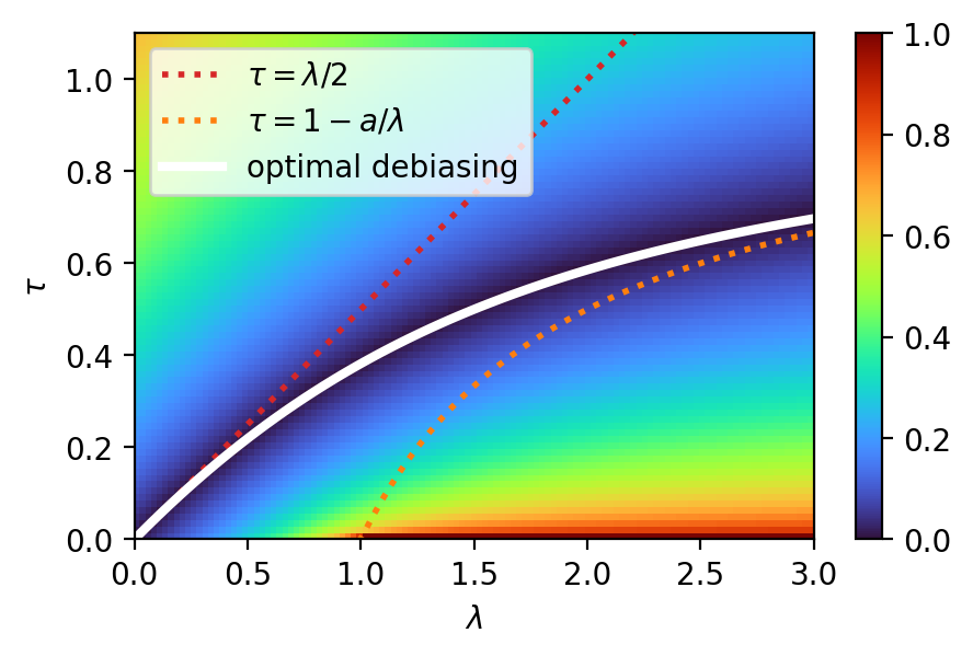
Figure 1: Wasserstein distance $d^{-1}W_{2}(\mu^{*}_{\lambda,\tau},\mu^{*}_{0,0})=(\sqrt{b}-\sqrt{a})^{2}$ between $\mu^{*}_{\lambda,\tau}$ and $\mu^{*}_{0,0}$ from (21), with $a=1.0$. The white line shows the best debiasing choice of $\tau^{*}(\lambda)$ from (22) for which this distance is $0$. Below this line the barycenter is shrinked and above it is blurred. Dashed lines show the small and large $\lambda$ asymptotics of $\tau^{*}(\lambda)$.

Non-asymptotic debiasing

As can be seen from (22), the choice $\tau=\lambda/2$ gives the optimal debiasing only asymptotically as $\lambda\to 0$. For larger values of $\lambda$, this formula suggests to use a value for $\tau$ that is smaller than $\lambda/2$; and in any case smaller than $1$. Remark that $\tau^{*}$ is concave and $\tau^{*}(\lambda)\leq\min\{\lambda/2,1\}$ (which are its tangents at $0$ and $\infty$) and that for $\lambda$ large it holds $\tau^{*}(\lambda)=1-a/\lambda+O((a/\lambda)^{3})$. In practice, one may use the outer regularization value $\tau^{*}(\lambda)$ as a heuristic even for non-gaussian measures, replacing $a$ by a notion of average of the variances of the marginals $\nu_{k}$.

	Objective	Variance (Isotropic Gaussian case)
$\mu_{0}^{*}$	$G_{0}$	$a$
$\mu_{\lambda,0}^{*}$	$G_{\lambda}$	$\max\{a-\lambda,0\}$
$\mu_{0,\tau}^{*}$	$G_{0}+\tau H$	$a+2\tau-\tau^{2}/a+O(\tau^{3}/a^{2})$
$\mu_{\lambda,\mathrm{div}}^{*}$	$G_{\lambda}-\frac{1}{2}T_{\lambda}(\cdot,\cdot)$	$a$
$\mu_{\lambda,\tau}^{*}$	$G_{\lambda}+\tau H$	$a+2\tau-\lambda+\tau(\lambda-\tau)/a+O((\lambda^{3}+\tau^{3})/a^{2})$
$\mu_{\lambda,\lambda/2}^{*}$	$G_{\lambda}+\frac{\lambda}{2}H$	$a+\lambda^{2}/(4a)+O(\lambda^{3}/a^{2})$

Table 2: Variance of $(\lambda,\tau)$-barycenters when the $\nu_{k}$ are Gaussians with variance $aI_{d}$ (Eq. (21)).

Barycenter of Dirac masses

Observe that for $a=0$, Eq. (21) gives $b=\tau$ (independently of $\lambda$). This can in fact be directly seen from the optimality conditions. Indeed, the Schrödinger system (7) gives that for each $k$, $\phi_{k}[{\mu^{*}_{\lambda,\tau}}](x)=\frac{1}{2}\|x-x_{k}\|^{2}-\psi_{k}$ for some $\psi_{k}\in\mathbb{R}$. Then the optimality condition (10) gives

$$\mu^{*}\propto e^{-\frac{\sum_{k}w_{k}\phi_{k}(x)}{\tau}}\propto e^{-\frac{\sum_{k}w_{k}\|x-x_{k}\|^{2}_{2}}{2\tau}}\propto e^{-\|x-\bar{x}\|^{2}/(2\tau)}.$$

The inner regularization $\lambda$ has no effect in this case because there is only one transport plan between any $\mu$ and each $\nu_{k}$ (in particular $\mu_{\lambda,0}^{*}=\mu^{*}_{0,0}$ for any $\lambda>0$).

3.3 Choice of the reference measure

As briefly mentioned in Section 1.2, there is an alternative formulation of $(\lambda,\tau)$-barycenters in terms of a change of reference measure in the definition of EOT. Let us develop this correspondance here. For a reference measure $\sigma\in\mathcal{M}_{+}(\mathcal{X}\times\mathcal{X})$, let

$$T_{\lambda}(\mu,\nu|\sigma) \coloneqq\min_{\gamma\in\Pi(\mu,\nu)}\int_{\mathcal{X}^{2}}c(x,y)\mathrm{d}\gamma(x,y)+\lambda H(\gamma|\sigma),$$ (23)

$$G_{\lambda}(\mu|\sigma_{\alpha}) \coloneqq\sum_{k=1}^{K}T_{\lambda}(\mu,\nu_{k}|\mu^{\alpha}\otimes\nu_{k}).$$ (24)

In the following discussion, $\mu^{\alpha}$ denotes $\mu$ itself when $\alpha=1$, the Lebesgue measure $\mathrm{d}x$ when $\alpha=0$ and $(\frac{\mathrm{d}\mu}{\mathrm{d}x})^{\alpha}$ otherwise. Note that one could equally choose $\sigma_{\alpha}=\mu^{\alpha}\otimes\tilde{\nu}_{k}$ for any $\tilde{\nu}_{k}$ such that $H(\nu_{k}|\tilde{\nu}_{k})$ is finite without changing the barycenter.

Lemma 3.5.

It holds

$$G_{\lambda}(\mu|\sigma_{\alpha})=G_{\lambda}(\mu)+\lambda(1-\alpha)H(\mu)$$

and for $\tau=\lambda(1-\alpha)$ the minimizer of this functional is $\mu^{*}_{\lambda,\tau}$.

Proof.

This is a consequence of the following property that can be found by direct computations (see [MG20, Lem. 1.6] for details): for any $\gamma\in\Pi(\mu,\nu)$ and $\alpha\in\mathbb{R}$, it holds

$$H(\gamma|\mu^{\alpha}\otimes\nu_{k})=H(\gamma|\mu\otimes\nu_{k})+(1-\alpha)H(\mu).\qed$$

This lemma is sufficient to justify the discussion after Def. 4. The effect of various choices of reference measure can be interpreted in view of the local expansion of Eq. (19) and are summarized in Table 3 (the two first rows correspond to cases discussed in [JCG20] for Gaussian measures). In the table, we used reference measures which are symmetric in $\mu,\nu$ as is standard, to fix ideas.

To conclude this section, let us insist on the fact that it is much more convenient to use the expression $F_{\lambda,\tau}=G_{\lambda}+\tau H$ as a sum of a smooth, convex functional and an entropy rather than $G_{\lambda}(\cdot|\sigma_{\alpha})$, although they are equivalent for $\tau=\lambda(1-\alpha)$. We rely on this decomposition in the next two sections.

Reference measure $\sigma$	Corresponding $\tau$	$1$st order bias term	Effect on barycenter
$\mathrm{d}x\otimes\mathrm{d}x$	$\tau=\lambda$	$\frac{\lambda}{2}H(\mu)$	Blurred
$\mu\otimes\nu$	$\tau=0$	$-\frac{\lambda}{2}H(\mu)$	Shrinked
$\sqrt{\mu}\otimes\sqrt{\nu}$	$\tau=\lambda/2$	$0$	Debiased
$\mu^{\alpha}\otimes\nu^{\alpha}$	$\tau=\lambda(1-\alpha)$	$\lambda(\frac{1}{2}-\alpha)$	–

Table 3: Effect of the choice of the reference measure and interpretation as a Dou-Ba. The bias refers to the error $G_{\lambda}(\mu|\sigma_{\alpha})-G_{0}(\mu)$ when $c(x,y)=\frac{1}{2}\|y-x\|^{2}_{2}$ (up to constant terms independent from $\mu$). In the last row, one needs $\alpha\leq 1$ so that $\tau\geq 0$.

4 Stability and statistical estimation

4.1 General stability result

The goal of this subsection is to prove the following general stability result, where the strongest point is (ii). In that statement, $W_{1}$ denotes the $L^{1}$-Wasserstein distance and $\dot{H}^{q}$ denotes the homogeneous Sobolev norm of order $q$.

Note that the first bound, adapted from [BCP19a, Thm. 3.3] does not require $\lambda>0$ and only exploits the first-order regularity of the cost while with $\lambda>0$, the barycenter is able to exploit the regularity of the cost to obtain stability under norms even weaker than $W_{1}$. Another stability result in the literature is [TK22, Thm. 1] which proves $\ell_{2}$-stability of $(\lambda,\lambda)$-barycenters in a discrete setting, under $\ell_{\infty}$ perturbations of the cost matrix (with an exponential dependence in $\lambda^{-1}$).

Before we start the proof, let us state a lemma that only uses convexity of $G_{\lambda}$; the lower-bound is classical and the upper-bound is used later in Section 5.

Lemma 4.2 (Entropy sandwich).

Let $\mu\in\mathcal{P}(\mathcal{X})$ and consider the “tangent Gibbs distribution” $\nu\propto\exp(-V[\mu]/\tau)$ where $V$ is the first-variation (9) of $G_{\lambda}$. It holds

$$\tau H(\mu|\mu_{\lambda,\tau})\leq F_{\lambda,\tau}(\mu)-F_{\lambda,\tau}(\mu^{*}_{\lambda,\tau})\leq\tau H(\mu|\nu).$$

Proof.

For brevity, let us write $F=F_{\lambda,\tau}$ and $\mu^{*}=\mu^{*}_{\lambda,\tau}$. By convexity of $G_{\lambda}$, we have

$$G_{\lambda}(\mu^{*})+\int V[\mu^{*}]\mathrm{d}(\mu-\mu^{*})\leq G_{\lambda}(\mu)\leq G_{\lambda}(\mu^{*})+\int V[\mu]\mathrm{d}(\mu-\mu^{*}).$$

Adding $\tau H(\mu)-G_{\lambda}(\mu^{*})-\tau H(\mu^{*})$ we get

$$\int V[\mu^{*}]\mathrm{d}(\mu-\mu^{*})+\tau H(\mu)-\tau H(\mu^{*})\leq F(\mu)-F(\mu^{*})\leq\int V[\mu]\mathrm{d}(\mu-\mu^{*})+\tau H(\mu)-\tau H(\mu^{*})$$

which is equivalent to

$$\tau H(\mu|\mu^{*})-\tau H(\mu^{*}|\mu^{*})\leq F(\mu)-F(\mu^{*})\leq\tau H(\mu|\nu)-\tau H(\mu^{*}|\nu)$$

using $\mu^{*}\propto e^{-V[\mu^{*}]/\tau}$ (Thm. 2.5). The claim follows from $H(\mu^{*}|\mu^{*})=0$ and $H(\mu^{*}|\nu)\geq 0$. ∎

Proof of Thm. 4.1.

Let us start with an application of the previous lemma (we put hats on the quantity defined using the empirical measures $(\hat{\nu}_{k})_{k=1}^{K}$):

$$\tau H(\hat{\mu}|\mu^{*}) \leq F(\hat{\mu})-F(\mu^{*})$$

$$=[F(\hat{\mu})-\hat{F}(\hat{\mu})]+[\hat{F}(\hat{\mu})-\hat{F}(\mu^{*})]+[\hat{F}(\mu^{*})-F(\mu^{*})]$$

$$\leq G_{\lambda}(\hat{\mu})-\hat{G}_{\lambda}(\hat{\mu})+0+\hat{G}_{\lambda}(\mu^{*})-G_{\lambda}(\mu^{*})$$

$$\leq\sum_{k=1}^{K}w_{k}\big{(}T_{\lambda}(\hat{\mu},\nu_{k})-T_{\lambda}(\hat{\mu},\hat{\nu}_{k})\big{)}+\sum_{k=1}^{K}w_{k}\big{(}T_{\lambda}(\mu^{*},\hat{\nu}_{k})-T_{\lambda}(\mu^{*},\nu_{k})\big{)}$$

$$\leq 2\sum_{k=1}^{K}w_{k}\sup_{\mu\in\mathcal{P}(\mathcal{X})}|T_{\lambda}(\mu,\hat{\nu}_{k})-T_{\lambda}(\mu,\nu_{k})|$$

Now by convexity of $T_{\lambda}$ in $\nu_{k}$, we have (denoting $\psi_{\mu,\nu}$ the Schrödinger potential from $\nu$ to $\mu$):

$$\int\psi_{\mu,\hat{\nu}_{k}}\mathrm{d}[\nu-\hat{\nu}]\leq T_{\lambda}(\mu,\nu_{k})-T_{\lambda}(\mu,\hat{\nu}_{k})\leq\int\psi_{\mu,\nu_{k}}\mathrm{d}[\nu-\hat{\nu}].$$

Given any norm $\|\cdot\|$ on the set of continuous functions defined up to constants, denoting $\|\sigma\|_{*}=\sup_{\|f\|\leq 1}\int f\mathrm{d}\sigma$ the dual norm on the space of signed measures with $0$ total mass, it follows

$$\tau H(\hat{\mu}|\mu^{*})\leq 2C\sum_{k=1}^{K}w_{k}\|\nu_{k}-\hat{\nu}_{k}\|_{*}$$

where $C=\sup_{\mu,\nu\in\mathcal{P}(\mathcal{X})}\|\psi_{\mu,\nu}\|$. Let us now consider the two claims separately.

(i) If $c(x,\cdot)$ is $L$-Lipschitz for all $x\in\mathcal{X}$, then it can be seen from the Schrödinger system (7) that $\psi_{\mu,\nu}$ is also $L$-Lipschitz. Taking the Lipschitz semi-norm $\|f\|=\sup_{x\neq y}\frac{|f(x)-f(y)|}{|y-x|}$, the dual of which is the Kantorovich-Rubinstein norm $\|\nu_{k}-\hat{\nu}_{k}\|_{*}=W_{1}(\nu_{k},\hat{\nu}_{k})$ gives the first claim.

(ii) If $c\in\tilde{\mathcal{C}}^{p}$ then by differentiating the Schrödinger system $p$ times it follows that $\psi_{\mu,\nu}$ is $p$ times differentiable with $\|\psi_{\mu,\nu}\|_{\tilde{\mathcal{C}}^{p}}\leq C(1+\lambda^{1-p})$ where $C>0$ is a constant deoending on the cost [GCBCP19]. Since $\mathcal{X}$ is assumed compact, it follows that the homogeneous Sobolev norm $\|\psi_{\mu,\nu}\|_{\dot{H}^{p}}$ admits the same bound (up to a constant depending on the diameter of $\mathcal{X}$). The conclusion follows from the fact that the norms $\dot{H}^{p}$ and $\dot{H}^{-p}$ are dual to each other. ∎

4.2 Estimation from independent samples

In this section, we consider the statistical properties $(\lambda,\tau)$-barycenters. Assume that we dispose of $n$ independent samples $x^{(k)}_{1},\dots,x^{(k)}_{n}$ from each of the marginals $\nu_{k}$. Let $\hat{\mu}_{\lambda}\in\mathcal{P}_{2}(\mathcal{X})$ be the the plug-in estimator of the barycenter, defined as the $(\lambda,\tau)$-barycenter between the empirical marginals $\hat{\nu}_{k}=\frac{1}{n}\sum_{i=1}^{n}\delta_{x_{i}^{(k)}}$.

Corollary 4.3.

Let $\tau,\lambda>0$, define $d^{\prime}=2\lfloor d/2\rfloor$ and assume that $c\in\mathcal{C}^{1+d^{\prime}/2}(\mathcal{X}\times\mathcal{X})$. Let $\hat{\mu}_{\lambda,\tau}$ be the empirical barycenter and $\mu^{*}_{\lambda,\tau}$ the population barycenter. Then there is $C>0$ independent of $(\nu_{k})_{k}$ such that

$$\mathbf{E}[H(\hat{\mu}_{\lambda,\tau}|\mu^{*}_{\lambda,\tau})]\leq C\tau^{-1}(1+\lambda^{-d^{\prime}/2})n^{-1/2}.$$

Proof.

We follow a strategy similar to that used for the sample complexity of EOT [GCBCP19]. In Thm. 4.1, one can replace the homogeneous Sobolev norm $\dot{H}^{-p}$ by the (larger) inhomogeneous norm $H^{-p}$. For $p=1+d^{\prime}/2$, it is known that $H^{p}$ is a Reproducible Kernel Hilbert space norm, and by standard empirical process theory results [BM02] one has

$$\mathbf{E}\|\hat{\nu}_{k}-\nu_{k}\|_{H^{-p}}\leq Cn^{-1/2}.\qed$$

Related work

To the best of our knowledge, this is the first estimation rate for an OT-like barycenter that does not suffer from the curse of dimensionality. The rate of estimation for $(0,\tau)$-barycenter was studied in [Big20], where the rate is cursed by the dimension because then the bound of Thm. 4.1-(i) involves the quantity $W_{1}(\nu_{k},\hat{\nu}_{k})$ which is of order $n^{-1/d}$ for $d>2$ [FG15]. In the same paper, they also studied $(\lambda,\lambda)$-barycenter but on a discrete space. The estimation of barycenters on discrete spaces is a rich topic but with a very different behavior [HKM23, HMZ22]. See [PZ19] for an introduction to statistical aspects of OT, including barycenters. We also note that there is a line of works (see e.g. [ALP20, LPRS22]) that studies the estimation of barycenters given marginals $(\nu_{k})_{k}$ sampled from a distribution in $\mathcal{P}(\mathcal{P}(\mathcal{X}))$ (as in (17)) which is a rich but different problem.

5 Optimization with Noisy Particle Gradient Descent

We consider the computation of $(\lambda,\tau)$-barycenters when the marginals $(\nu_{k})_{k}$ are discrete with $n$ atoms each. In this case, the size of the problem is given by $n$ (the number of atoms), $K$ (the number of marginals) and $d$ (the ambiant dimension).

For small scale problems where one of these quantities is small, plenty of algorithms from the literature exist. For instance when $n$ or $K$ is small, one can directly solve a linear program of size $O(n^{K})$ – the multimarginal formulation [AC11] – to compute the $(0,0)$-barycenter. When $d$ is small, there exists efficient exact methods [AB21]. In that case, an alternative is to discretize the space, and use convex optimization algorithms to solve Eq. (4). This includes approaches based on linear programming [ABM16, GWXY19], entropic regularization [CD14, BCCNP15] or decentralized and randomized algorithms [DDGUN18, SCSJ17, HMZ22], see [PC19] for a review. This approach also applies for $(\lambda,\tau)$-barycenters (we compute 1D barycenters with this method in Section 6).

In this section, we focus on large scale problems ($n,d,K\gg 1$) where these discrete approaches are intractable and “free support” methods become relevant. A stream of recent work proposed methods based on neural networks [KLSB20, CAD20, LGYS20, FTC20]. These methods come with the advantages (useful statistical prior, reasonable iteration complexity) and the drawbacks (lack of optimization guarantees) of neural networks. Particle-based methods, which are closer in spirit to what follows, have been proposed such as fixed-point methods akin to Loyd’s algorithm [ÁDCM16, CCS18, Lin23, BFRT22a] and a particle gradient method [DGLT21] for Wasserstein barycenters. Note that it is shown in [AB22] that Wasserstein barycenters are NP-hard to compute in large dimension. A Franck-Wolfe algorithm [LSPC19] was proposed for Sinkhorn divergence barycenters.

In what follows, we propose a grid-free numerical method which is particularly well-suited to the structure of the problem of Eq. (4), called Noisy Particle Gradient Descent (NPGD). We defer a detailed complexity analysis of this method to future works, and limit ourselves to a introduction of the algorithm with its exponential guaranty in the mean-field limit, which is an application of [Chi22, NWS22].

5.1 Noisy Particle Gradient Descent

We parameterize the unknown measure as a mixture of $m\in\mathbb{N}^{*}$ particles $\hat{\mu}=\frac{1}{m}\sum_{i=1}^{m}\delta_{X_{j}}$. Let $\mathbf{X}=(X_{1},\dots,X_{m})\in(\mathbb{R}^{d})^{m}$ encode the position of all particles and consider the function

$$G_{m}(\mathbf{X})\coloneqq G_{\lambda}\Big{(}\frac{1}{m}\sum_{i=1}^{m}\delta_{X_{j}}\Big{)}.$$ (25)

The NPGD algorithm we consider is simply noisy gradient descent on $G_{m}$, with an initialization sampled from some $\mu_{0}\in\mathcal{P}(\mathcal{X})$. It is defined, for $\ell\in\mathbb{N}$, as

$$\mathbf{X}[\ell+1]=\mathsf{P}_{\mathcal{X}}\big{(}\mathbf{X}[\ell]-m\eta\nabla G_{m}(\mathbf{X}[\ell])+\sqrt{2\eta\tau}\mathbf{Z}[\ell]\big{)},\quad\mathbf{X}[0]\sim\mu_{0}^{\otimes m}$$ (26)

where $\tau>0$ is the outer-regularization strength, $\eta>0$ is the step-size, $\mathbf{Z}[1],\mathbf{Z}[2],\dots$ are i.i.d. standard Gaussian vectors and $\mathsf{P}_{\mathcal{X}}$ is the Euclidean projection on $\mathcal{X}$. Note that to compute $\nabla G_{m}$ one needs to solve, at each iteration, $K$ regularized optimal transport problems. In the small step-size limit $\eta\to 0$ and setting $t=k\eta$, NPGD leads to a system of SDEs coupled via the empirical distribution of particles $\hat{\mu}_{t}$:

$$\left\{\begin{aligned} \mathrm{d}X_{i}(t)&=-\nabla V[\hat{\mu}_{t}](X_{i}(t))\mathrm{d}t+\sqrt{2\tau}\mathrm{d}B_{t,i}+\mathrm{d}\Phi_{t,i},\quad X_{i}(0)\sim\mu_{0}\\ \hat{\mu}_{t}&=\frac{1}{m}\sum_{i=1}^{m}\delta_{X_{i}(t)}\end{aligned}\right.$$ (27)

where $(B_{t,i})_{t\geq 0}$ are independent Brownian motions in $\mathbb{R}^{d}$, $\mathrm{d}\Phi_{t,i}$ is a boundary reflection (in the sense of Skorokhod problem) and $V[\mu]\in\mathcal{C}^{1}(\mathcal{X})$ is the first-variation of $G_{\lambda}$ at $\mu$ (see Definition 9). The latter satisfies $V[\hat{\mu}](X_{i})=m\nabla_{X_{i}}G_{m}(\mathbf{X})$, hence (26) is just the Euler-Maruyama discretization of (27) below.

5.2 Mean-Field Langevin dynamics

In the many-particle $m\to\infty$ limit, it can be shown that the particles behave like independent sample paths from the nonlinear SDE of McKean-Vlasov type:

$$\left\{\begin{aligned} \mathrm{d}X_{t}&=-\nabla V[\mu_{t}](X(t))\mathrm{d}t+\sqrt{2\tau}\mathrm{d}B_{t}+\mathrm{d}\Phi_{t},\quad X_{0}\sim\mu_{0}\\ \mu_{t}&=\mathrm{Law}(X_{t})\end{aligned}\right.$$ (28)

where $(B_{t})_{t\geq 0}$ is a Brownian motion and $(\Phi_{t})_{t\geq 0}$ a boundary reflection. Moreover, the distribution $(\mu_{t})_{t\geq 0}$ of particles solves the evolution equation

$$\partial_{t}\mu_{t}=\nabla\cdot\big{(}\mu_{t}\nabla V_{\lambda}[\mu_{t}]\big{)}+\tau\Delta\mu_{t}$$ (29)

starting from $\mu_{0}\in\mathcal{P}(\mathcal{X})$ where $\nabla\cdot$ stands for the divergence operator. By solution of (29) here, we mean an curve $(\mu_{t})_{t\geq 0}$ starting from $\mu_{0}$ that is absolutely continuous in Wasserstein space and satisfies Eq. (29) in the sense of distributions with no-flux boundary conditions.

This drift-diffusion equation is an instance of Mean-Field Langevin dynamics, a class of drift-diffusion dynamics studied in [MMN18, HRŠS21, NWS22, Chi22]. It can be interpreted as the gradient flow of the functional $F_{\lambda}$ of Eq. (4) under the $W_{2}$ Wasserstein metric.

In our theoretical analysis, we focus on the analysis of the mean-field limit (29). For quantitative convergence results in the many-particle $m\to\infty$ and small step-size $\eta\to 0$ limits, one can refer to the classical work [Szn91]. The particular case of reflecting boundary conditions has been treated in [JMM20], following earlier works on the analysis of SDEs with reflection [Tan79, LS84].

5.3 Exponential convergence

It has been shown independently in [NWS22] and [Chi22] that if the function $G_{\lambda}$ is convex, regular enough and that a certain family of log-Sobolev inequalities holds, then dynamics of the form Eq. (29) converge at an exponential rate to the unique minimizer of $F_{\lambda}$. Let us apply this result in our context, where this leads to a dynamics that directly converges to the $(\lambda,\tau)$-barycenter.

Proof.

We have semi-convexity of $F_{\lambda,\tau}$ along Wasserstein geodesics, by [CCM22, Thm. 4.1] for the first component $G_{\lambda}$ and by a standard result [San15] for the $H$ component. Thus the general well-posedness results from [AGS05] applies. For the exponential convergence – in function value and in relative entropy – we apply the result from [Chi22, Thm. 3.2], see also [NWS22] where the same argument was discovered independently (although stated on $\mathbb{R}^{d}$, the argument goes through on a compact domain).

The main assumptions to check are that (i) $\mu\mapsto G_{\lambda}(\mu)$ is convex (Prop. 2.3), (ii) that a global minimizer $\mu^{*}_{\lambda,\tau}$ exists (Thm. 2.5) and finally we need to check that the probability measure $\hat{\mu}_{t}\propto e^{-V[\mu_{t}]}\in\mathcal{P}(\mathcal{X})$ satisfies a log-Sobolev inequality, uniformly in $t$ (Assumption 3 in [Chi22]).

Since $\mathcal{X}$ is bounded, the normalized Lebesgue measure satisfies a log-Sobolev inequality [Led99, Thm. 7.3]. By the Holley-Stroock perturbation criterion [HS86] $\hat{\mu}_{t}$ satisfies it as well; this criterion applies here because $\sup_{x}V[\mu](x)-\inf_{x}V[\mu](x)$ is bounded, uniformly in $\mu\in\mathcal{P}(\mathcal{X})$ by Prop. 2.3. ∎

The contraction rate $\rho_{\lambda}$ is of the form $\tau e^{-L\cdot\mathrm{diam}(\mathcal{X})/\tau}$ where $L$ is the Lipschitz constant of $c$ (and $L\cdot\mathrm{diam}(\mathcal{X})$ is a uniform bound on $\|V[\mu]\|_{\mathrm{osc}}$). It thus approaches $1$ exponentially fast as $\tau$ decreases. We also note that both inner and outer regularizations are needed to obtain Thm. 5.1: in particular the inner-regularization is necessary to obtain well-posedness of the PDE (29).

6 Numerical experiments

The (Julia) code to reproduce the experiments is available online.

Comparison of 1D-barycenters

On Fig. 2 we compare various barycenters for $K=3$ and $(\nu_{k})_{k=1}^{3}$ probability densities on $\mathcal{X}=[0,1]$ with cost $c(x,y)=\nicefrac{{1}}{{2}}\|y-x\|^{2}_{2}$. The $(\lambda,\tau)$-barycenters have been computed numerically using gradient ascent in $L^{2}(w_{1}\nu_{1})\times\dots L^{2}(w_{K}\nu_{K})$ on the smooth dual (12) after discretizing the problem on a regular grid of size $200$. The algorithm converged linearly for small enough step-sizes. For reference, we plot in blue the unregularized Wasserstein barycenter $\mu^{*}_{0,0}$ that is computed by taking the $L^{2}$-barycenter of the quantile functions [San15, Chap. 2]. We observe that the choice $\tau=\lambda/2$ indeed gives the best approximation of $\mu^{*}_{0,0}$ for fixed $\lambda$. For comparison, we also plot the Sinkhorn divergence barycenter $\mu^{*}_{\lambda,\mathrm{div}}$, which is computed with [JCG20, Alg. 1]. We observe that it also approaches weakly $\mu^{*}_{0,0}$ but its density displays strong oscillations, suggesting that this object is in general less well-behaved than $(\lambda,\tau)$-barycenters.

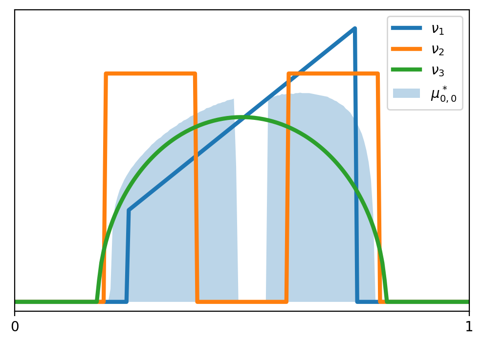
(a) Densities $(\nu_{k})_{k=1}^{3}$ and $\mu^{*}_{0,0}$

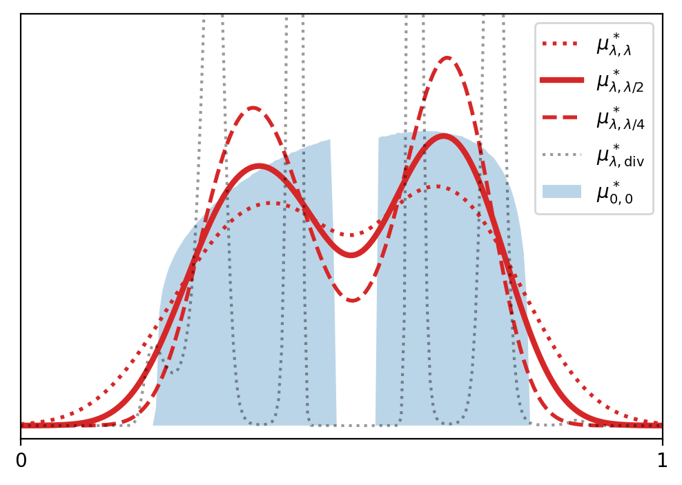
(b) $\lambda=1/128$

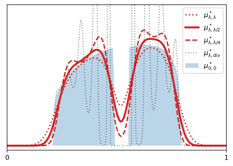
(c) $\lambda=1/512$

Figure 2: Iso-barycenters for $(\nu_{k})_{k=1}^{3}$ probability densities on $\mathcal{X}=[0,1]$ (displayed on the left). For $\lambda,\tau>0$, $\mu^{*}_{\lambda,\tau}$ is computed with gradient ascent on the discretized dual problem.

Escaping stationary points with noisy particle gradient descent

To illustrate the global convergence of Noisy Particle Gradient Descent (NPGD) to $\mu^{*}_{\lambda,\tau}$ in the mean-field limit, we consider a configuration for which $G_{0}$ has a “bad” local minimum and initialize the dynamics at this measure as shown on Fig. 3(a). We consider on $\mathcal{X}=\mathbb{R}^{2}$ the barycenter of

$$\nu_{1}=\frac{1}{2}(\delta_{(-3,0)}+\delta_{(-1,1)}) \nu_{2}=\frac{1}{2}(\delta_{(1,1)}+\delta_{(3,1)})$$ and

with cost $c(x,y)=\frac{1}{2}\|y-x\|^{2}_{2}$. It can be checked with direct computations that $\mu^{*}_{(0,0)}=\frac{1}{2}(\delta_{(-1,\nicefrac{{1}}{{2}})}+\delta_{(1,\nicefrac{{1}}{{2}})})$ and that the measure $\mu^{*}_{\mathrm{init}}=\frac{1}{2}(\delta_{(0,0)}+\delta_{(0,1)})$ is a stable local minimizer (in the sense that when parameterized by the positions of these two Dirac masses, $G_{0}$ is locally minimized by $((0,0),(0,1))$ and its Hessian at this point is positive definite, proportional to the identity). In particular, fixed-point or gradient descent iterations for $G_{0}$ would not move from this stationary point. On Fig. 3(a) we observe, in accordance to Thm. 5.1, that NPGD can escape from the neighborhood of $\mu_{\mathrm{init}}$ and converge to a discrete approximation of $\mu^{*}_{(\lambda,\lambda/2)}$, itself an approximation of $\mu^{*}_{(0,0)}$. Note that this is only observed when $\tau$ is large enough, otherwise the dynamics is trapped in “metastable” states (here $\lambda=0.1$ and $\tau=\lambda/2$). We have used $m=200$ particles, a step-size of $0.5$ and Fig. 3(a) represents the state of NPGD after $400$ iterations.

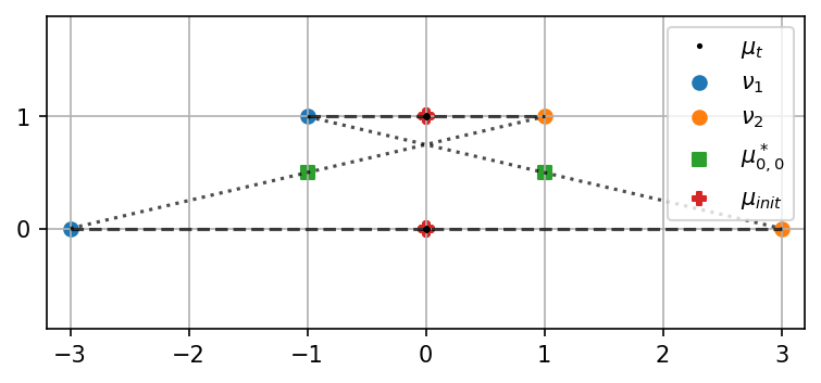
(a) Initializing on a local minimum of $G_{0}$ ($t=0$)

(b) Approximate global minimizer ($t$ large)

Figure 3: Illustration of the global convergence of the noisy particle gradient descent algorithm. (left) We initialize $m=200$ particles on the measure $\mu_{\mathrm{init}}$ which is a local minimizer of $G_{0}$. (right) The algorithm converges to a distribution which approximates $\mu^{*}_{\lambda,\lambda/2}$, itself a small convolution of $\mu^{*}_{0,0}$.

7 Conclusion

We have proposed doubly-regularized EOT barycenters which is a formulation of barycenters over $\mathcal{P}(\mathcal{X})$ that has several benefits: (i) it gathers most previously studied OT-like barycenters in a single framework, (ii) it leads to several desirable properties such as regularity, stability and approximation of Wasserstein barycenters (for $\tau=\lambda/2$), and (iii) it lends itself naturally to both convex optimization methods and grid-free methods.

In this paper, we have covered a diverse range of theoretical topics (regularity, approximation, statistics, optimization) as it is really all these aspects that together make this family of objects stand out. In future work, it will be desirable to develop in depth analyses of specialized points, such as the computational complexity of $(\lambda,\tau)$-barycenters.

Appendix A Closed forms for isotropic Gaussians

In this section, we consider the simplest setting of centered isotropic Gaussian probability measures and rely on closed forms for entropic optimal transport. We consider

$$\min_{\nu\in\mathcal{P}(\mathbb{R}^{d})}T_{\lambda}(\mu,\nu)+\tau H(\nu)$$ (30)

for $\mu=\mathcal{N}(0,a)$ where $a>0$ is the variance. This is enough to recover the general case of barycenters of isotropic Gaussians with identical variances since the effect of having different means can be factored out as in [JMPC20]. Note that [BBB20] also considered this problem but did not obtain a closed form solution. Let us look for a Gaussian solution of the form $\nu=\mathcal{N}(0,b)$. By [JMPC20], we have that the optimal dual potentials are $\varphi=\frac{1}{2}\tilde{u}\|x\|_{2}^{2}$ and $\psi=\frac{1}{2}\tilde{v}\|y\|^{2}$ with

$$\tilde{u} =1-\frac{2b}{\xi+\lambda}, \tilde{v} =1-\frac{2a}{\xi+\lambda}, \xi =\sqrt{4ab+\lambda^{2}}$$

where the variables from [JMPC20] and our variables are related by $\sigma^{2}\rightarrow\lambda$, $U\rightarrow-\lambda\tilde{u}I$, $V\rightarrow-\lambda\tilde{v}I$, $C\rightarrow I\cdot(\xi-\lambda)/2$. Also the EOT cost and entropy is

$$\frac{2}{d}T_{\lambda}(\mu,\nu) =a+b-\xi+\lambda\log(\xi+\lambda)+C, \frac{2}{d}\tau H(\mu) =-\tau\log(b)+C$$

where $C$ denotes a constant independent of $a$ and $b$. When restricted to $\nu$ of the form $\mathcal{N}(0,b)$, the optimization problem thus becomes (keeping in mind that $\xi$ depends on $b$)

$$\min_{b>0}a+b-\xi+\lambda\log(\xi+\lambda)-\tau\log(b).$$

The first order optimality condition reads

$$1-\frac{2a}{\xi+\lambda}-\frac{\tau}{b}=0$$ (31)

Now, let us argue that if $b$ satisfies this equation, then $\nu$ is in fact the unique minimizer of (30). Indeed, (30) admits a unique solution characterized by the first order optimality condition (which can be justified, in this non-compact setting, as in [JMPC20]):

$$\log\Big{(}\frac{\mathrm{d}\nu}{\mathrm{d}x}\Big{)}+\frac{\psi_{\mu,\nu}}{\tau}=C$$

But if $\nu=\mathcal{N}(0,b)$ with $b$ solution to (31) then it holds

$$\tilde{v} =\tau/b \Rightarrow \frac{\psi_{\mu,\nu}(y)}{\tau}-\frac{\|y\|^{2}_{2}}{2b}=0$$ (32)

which proves that $\nu$ is indeed the unique solution to our problem.

Explicit solution.

Using $b=(\xi^{2}-\lambda^{2})/(4a)$, let us express (31) in terms of $\xi$:

$$b(\xi+\lambda)-2ab-\tau(\xi+\lambda)=0\Leftrightarrow\frac{\xi+\lambda}{4a}(\xi^{2}-2a\xi-\lambda^{2}+2a\lambda-4a\tau)=0.$$

Solving for $\xi$ and taking the largest solution (which must be the unique solution leading to $b\geq 0$) leads to

$$\xi=a+\sqrt{(a-\lambda)^{2}+4a\tau} \Rightarrow b=\frac{\big{(}a+\sqrt{(a-\lambda)^{2}+4a\tau}\big{)}^{2}-\lambda^{2}}{4a}.$$

Let us now consider some particular cases:

• In the limit $\tau\to 0$, we have

  $$b=\frac{(a+|a-\lambda|)^{2}-\lambda^{2}}{4a}=\begin{cases}a-\lambda&\text{if $a>\lambda$}\\ 0&\text{if $a\leq\lambda$}\end{cases}$$

• In the limit $\lambda\to 0$, we have

  $$b=\frac{a}{4}\big{(}1+\sqrt{1+4\tau/a}\big{)}^{2}=a+2\tau+O(\tau^{2})$$

• for $\tau=\lambda$, we have

  $$b=\frac{(a+|a+\lambda|)^{2}-\lambda^{2}}{4a}=a+\lambda$$

• for $\tau=\lambda/2$, we have

  $$b =\frac{(a+\sqrt{a^{2}+\lambda^{2}})^{2}-\lambda^{2}}{4a}$$

  $$=\frac{a^{2}+a^{2}+\lambda^{2}+2a\sqrt{a^{2}+\lambda^{2}}-\lambda^{2}}{4a}$$

  $$=\frac{2a^{2}+2a^{2}\sqrt{1+(\lambda/a)^{2}}}{4a}$$

  $$=\frac{a}{2}(1+\sqrt{1+(\lambda/a)^{2}})=a+\frac{\lambda^{2}}{4a}+O(\lambda^{4})$$

Best choice of $\tau$

Let us now solve for $\tau$ such that $b=a$, which we know is asymptotically $\tau\sim\lambda/2$. It holds

$$b-a=0 \Leftrightarrow (a+\sqrt{(a-\lambda)^{2}+4a\tau})^{2}-\lambda^{2}-4a^{2}=0.$$

Let us define the intermediate unknown $\chi=\sqrt{(a-\lambda)^{2}+4a\tau}\Leftrightarrow\tau=(\chi^{2}-(a-\lambda)^{2})/(4a)$. It follows

$$(a+\chi)^{2}-\lambda^{2}-4a^{2}=0 \Leftrightarrow \chi^{2}+2a\chi-\lambda^{2}-3a^{2}=0.$$

Solving for $\chi$, with the constraint $\chi\geq 0$ gives

$$\chi=\sqrt{4a^{2}+\lambda^{2}}-a \Leftrightarrow \tau=\frac{(\sqrt{4a^{2}+\lambda^{2}}-a)^{2}-(a-\lambda)^{2}}{4a}.$$

Developing the squares and rearranging we get

$$\tau =\frac{4a^{2}+-2a\sqrt{4a^{2}+\lambda^{2}}+2a\lambda}{4a}$$

$$=\frac{\lambda}{2}+a\Big{(}1-\Big{(}1+\frac{\lambda^{2}}{4a^{2}}\Big{)}^{1/2}\Big{)}$$

$$=\frac{\lambda}{2}-\frac{\lambda^{2}}{8a}+O(\lambda^{4}/a^{3}).$$

References

- [AB21] Jason M. Altschuler and Enric Boix-Adsera “Wasserstein barycenters can be computed in polynomial time in fixed dimension” In The Journal of Machine Learning Research 22.1 JMLRORG, 2021, pp. 2000–2018
- [AB22] Jason M. Altschuler and Enric Boix-Adsera “Wasserstein barycenters are NP-hard to compute” In SIAM Journal on Mathematics of Data Science 4.1 SIAM, 2022, pp. 179–203
- [ABM16] Ethan Anderes, Steffen Borgwardt and Jacob Miller “Discrete Wasserstein barycenters: Optimal transport for discrete data” In Mathematical Methods of Operations Research 84.2 Springer, 2016, pp. 389–409
- [AC11] Martial Agueh and Guillaume Carlier “Barycenters in the Wasserstein space” In SIAM Journal on Mathematical Analysis 43.2 SIAM, 2011, pp. 904–924
- [AC17] Martial Agueh and Guillaume Carlier “Vers un théorème de la limite centrale dans l’espace de Wasserstein?” In Comptes Rendus Mathématique 355.7 Elsevier, 2017, pp. 812–818
- [ÁDCM16] Pedro C. Álvarez-Esteban, E. Del Barrio, J.A. Cuesta-Albertos and C. Matrán “A fixed-point approach to barycenters in Wasserstein space” In Journal of Mathematical Analysis and Applications 441.2 Elsevier, 2016, pp. 744–762
- [AGS05] Luigi Ambrosio, Nicola Gigli and Giuseppe Savaré “Gradient flows: in metric spaces and in the space of probability measures” Springer Science & Business Media, 2005
- [ALP20] Adil Ahidar-Coutrix, Thibaut Le Gouic and Quentin Paris “Convergence rates for empirical barycenters in metric spaces: curvature, convexity and extendable geodesics” In Probability theory and related fields 177.1-2 Springer, 2020, pp. 323–368
- [BBB20] Marin Ballu, Quentin Berthet and Francis Bach “Stochastic optimization for regularized Wasserstein estimators” In International Conference on Machine Learning, 2020, pp. 602–612 PMLR
- [BBR06] Federico Bassetti, Antonella Bodini and Eugenio Regazzini “On minimum Kantorovich distance estimators” In Statistics & probability letters 76.12 Elsevier, 2006, pp. 1298–1302
- [BCCNP15] Jean-David Benamou, Guillaume Carlier, Marco Cuturi, Luca Nenna and Gabriel Peyré “Iterative Bregman projections for regularized transportation problems” In SIAM Journal on Scientific Computing 37.2 SIAM, 2015, pp. A1111–A1138
- [BCP19] Jérémie Bigot, Elsa Cazelles and Nicolas Papadakis “Data-driven regularization of Wasserstein barycenters with an application to multivariate density registration” In Information and Inference: A Journal of the IMA 8.4 Oxford University Press, 2019, pp. 719–755
- [BCP19a] Jérémie Bigot, Elsa Cazelles and Nicolas Papadakis “Penalization of barycenters in the Wasserstein space” In SIAM Journal on Mathematical Analysis 51.3 SIAM, 2019, pp. 2261–2285
- [BFRT22] Julio Backhoff-Veraguas, Joaquin Fontbona, Gonzalo Rios and Felipe Tobar “Bayesian learning with Wasserstein barycenters” In ESAIM: Probability and Statistics 26 EDP Sciences, 2022, pp. 436–472
- [BFRT22a] Julio Backhoff-Veraguas, Joaquin Fontbona, Gonzalo Rios and Felipe Tobar “Stochastic gradient descent in Wasserstein space” In arXiv preprint arXiv:2201.04232, 2022
- [Big20] Jérémie Bigot “Statistical data analysis in the Wasserstein space” In ESAIM: Proceedings and Surveys 68 EDP Sciences, 2020, pp. 1–19
- [BJGR19] Espen Bernton, Pierre E. Jacob, Mathieu Gerber and Christian P Robert “On parameter estimation with the Wasserstein distance” In Information and Inference: A Journal of the IMA 8.4 Oxford University Press, 2019, pp. 657–676
- [BL20] Eustasio Barrio and Jean-Michel Loubes “The statistical effect of entropic regularization in optimal transportation” In arXiv preprint arXiv:2006.05199, 2020
- [BLL15] Emmanuel Boissard, Thibaut Le Gouic and Jean-Michel Loubes “Distribution’s template estimate with Wasserstein metrics” In Bernoulli 21.2 Bernoulli Society for Mathematical StatisticsProbability, 2015, pp. 740–759
- [BM02] Peter Bartlett and Shahar Mendelson “Rademacher and Gaussian complexities: Risk bounds and structural results” In Journal of Machine Learning Research 3.Nov, 2002, pp. 463–482
- [BV04] Stephen Boyd and Lieven Vandenberghe “Convex optimization” Cambridge university press, 2004
- [CAD20] Samuel Cohen, Michael Arbel and Marc Peter Deisenroth “Estimating barycenters of measures in high dimensions” In arXiv preprint arXiv:2007.07105, 2020
- [CCM22] Guillaume Carlier, Lénaïc Chizat and Laborde Maxime “Lipschitz continuity of Schödinger’s map” In in preparation, 2022
- [CCS18] Sebastian Claici, Edward Chien and Justin Solomon “Stochastic Wasserstein barycenters” In International Conference on Machine Learning, 2018, pp. 999–1008 PMLR
- [CD14] Marco Cuturi and Arnaud Doucet “Fast computation of Wasserstein barycenters” In International conference on machine learning, 2014, pp. 685–693 PMLR
- [CDM22] Guillaume Carlier, Alex Delalande and Quentin Merigot “Quantitative Stability of Barycenters in the Wasserstein Space” In arXiv preprint arXiv:2209.10217, 2022
- [CEK21] Guillaume Carlier, Katharina Eichinger and Alexey Kroshnin “Entropic-Wasserstein barycenters: PDE characterization, regularity, and CLT” In SIAM Journal on Mathematical Analysis 53.5 SIAM, 2021, pp. 5880–5914
- [CGP16] Yongxin Chen, Tryphon T. Georgiou and Michele Pavon “On the relation between optimal transport and Schrödinger bridges: A stochastic control viewpoint” In Journal of Optimization Theory and Applications 169 Springer, 2016, pp. 671–691
- [Chi22] Lénaïc Chizat “Mean-Field Langevin Dynamics: Exponential Convergence and Annealing” In Transactions on Machine Learning Research, 2022
- [CMRS20] Sinho Chewi, Tyler Maunu, Philippe Rigollet and Austin J. Stromme “Gradient descent algorithms for Bures-Wasserstein barycenters” In Conference on Learning Theory, 2020, pp. 1276–1304 PMLR
- [CP18] Marco Cuturi and Gabriel Peyré “Semidual regularized optimal transport” In SIAM Review 60.4 SIAM, 2018, pp. 941–965
- [CRLVP20] Lénaïc Chizat, Pierre Roussillon, Flavien Léger, François-Xavier Vialard and Gabriel Peyré “Faster Wasserstein Distance Estimation with the Sinkhorn Divergence” In Neural Information Processing Systems, 2020
- [CT21] Giovanni Conforti and Luca Tamanini “A formula for the time derivative of the entropic cost and applications” In Journal of Functional Analysis 280.11 Elsevier, 2021, pp. 108964
- [Cut13] Marco Cuturi “Sinkhorn distances: Lightspeed computation of optimal transport” In Advances in Neural Information Processing Systems 26, 2013
- [DDGUN18] Pavel Dvurechenskii, Darina Dvinskikh, Alexander Gasnikov, Cesar Uribe and Angelia Nedich “Decentralize and Randomize: Faster Algorithm for Wasserstein Barycenters” In Advances in Neural Information Processing Systems 31, 2018
- [DGLT21] Chiheb Daaloul, Thibaut Le Gouic, Jacques Liandrat and Magali Tournus “Sampling from the Wasserstein barycenter” In arXiv preprint arXiv:2105.01706, 2021
- [DLR13] Manh Hong Duong, Vaios Laschos and Michiel Renger “Wasserstein gradient flows from large deviations of many-particle limits” In ESAIM: Control, Optimisation and Calculus of Variations 19.4 EDP Sciences, 2013, pp. 1166–1188
- [EMR15] Matthias Erbar, Jan Maas and Michiel Renger “From large deviations to Wasserstein gradient flows in multiple dimensions”, 2015
- [ES90] Sven Erlander and Neil F. Stewart “The gravity model in transportation analysis: theory and extensions” Vsp, 1990
- [Fey+19] Jean Feydy, Thibault Séjourné, François-Xavier Vialard, Shun-ichi Amari, Alain Trouvé and Gabriel Peyré “Interpolating between optimal transport and MMD using Sinkhorn divergences” In The 22nd International Conference on Artificial Intelligence and Statistics, 2019, pp. 2681–2690 PMLR
- [FG15] Nicolas Fournier and Arnaud Guillin “On the rate of convergence in Wasserstein distance of the empirical measure” In Probability theory and related fields 162.3-4 Springer, 2015, pp. 707–738
- [FTC20] Jiaojiao Fan, Amirhossein Taghvaei and Yongxin Chen “Scalable Computations of Wasserstein Barycenter via Input Convex Neural Networks” In arXiv e-prints, 2020, pp. arXiv–2007
- [GCBCP19] Aude Genevay, Lénaïc Chizat, Francis Bach, Marco Cuturi and Gabriel Peyré “Sample complexity of Sinkhorn divergences” In The 22nd International Conference on Artificial Intelligence and Statistics, 2019, pp. 1574–1583 PMLR
- [GWXY19] DongDong Ge, Haoyue Wang, Zikai Xiong and Yinyu Ye “Interior-Point Methods Strike Back: Solving the Wasserstein Barycenter Problem” In Advances in Neural Information Processing Systems 32, 2019, pp. 6894–6905
- [HKM23] Florian Heinemann, Marcel Klatt and Axel Munk “Kantorovich–Rubinstein Distance and Barycenter for Finitely Supported Measures: Foundations and Algorithms” In Applied Mathematics & Optimization 87.1 Springer, 2023, pp. 4
- [HMZ22] Florian Heinemann, Axel Munk and Yoav Zemel “Randomized Wasserstein Barycenter Computation: Resampling with Statistical Guarantees” In SIAM Journal on Mathematics of Data Science 4.1 SIAM, 2022, pp. 229–259
- [HRŠS21] Kaitong Hu, Zhenjie Ren, David Šiška and Łukasz Szpruch “Mean-field Langevin dynamics and energy landscape of neural networks” In Annales de l’Institut Henri Poincare (B) Probabilites et statistiques 57.4, 2021, pp. 2043–2065 Institut Henri Poincaré
- [HS86] Richard Holley and Daniel W. Stroock “Logarithmic Sobolev inequalities and stochastic Ising models” Laboratory for InformationDecision Systems, Massachusetts Institute of …, 1986
- [JCG20] Hicham Janati, Marco Cuturi and Alexandre Gramfort “Debiased Sinkhorn barycenters” In International Conference on Machine Learning, 2020, pp. 4692–4701 PMLR
- [JMM20] Adel Javanmard, Marco Mondelli and Andrea Montanari “Analysis of a two-layer neural network via displacement convexity” In The Annals of Statistics 48.6 Institute of Mathematical Statistics, 2020, pp. 3619–3642
- [JMPC20] Hicham Janati, Boris Muzellec, Gabriel Peyré and Marco Cuturi “Entropic optimal transport between unbalanced Gaussian measures has a closed form” In Advances in neural information processing systems 33, 2020, pp. 10468–10479
- [KLSB20] Alexander Korotin, Lingxiao Li, Justin Solomon and Evgeny Burnaev “Continuous Wasserstein-2 Barycenter Estimation without Minimax Optimization” In International Conference on Learning Representations, 2020
- [KP17] Young-Heon Kim and Brendan Pass “Wasserstein barycenters over Riemannian manifolds” In Advances in Mathematics 307 Elsevier, 2017, pp. 640–683
- [Kro+19] Alexey Kroshnin, Nazarii Tupitsa, Darina Dvinskikh, Pavel Dvurechensky, Alexander Gasnikov and Cesar Uribe “On the complexity of approximating Wasserstein barycenters” In International conference on machine learning, 2019, pp. 3530–3540 PMLR
- [KY94] Jeffrey J. Kosowsky and Alan L. Yuille “The invisible hand algorithm: Solving the assignment problem with statistical physics” In Neural networks 7.3 Elsevier, 1994, pp. 477–490
- [Led99] Michel Ledoux “Concentration of measure and logarithmic Sobolev inequalities” In Seminaire de probabilités XXXIII Springer, 1999, pp. 120–216
- [Léo12] Christian Léonard “From the Schrödinger problem to the Monge–Kantorovich problem” In Journal of Functional Analysis 262.4 Elsevier, 2012, pp. 1879–1920
- [LGYS20] Lingxiao Li, Aude Genevay, Mikhail Yurochkin and Justin Solomon “Continuous Regularized Wasserstein Barycenters” In Advances in Neural Information Processing Systems 33, 2020
- [Lin23] Johannes von Lindheim “Simple approximative algorithms for free-support Wasserstein barycenters” In Computational Optimization and Applications Springer, 2023, pp. 1–34
- [LPRS22] Thibaut Le Gouic, Quentin Paris, Philippe Rigollet and Austin Stromme “Fast convergence of empirical barycenters in Alexandrov spaces and the Wasserstein space” In Journal of the European Mathematical Society, 2022
- [LS84] Pierre-Louis Lions and Alain-Sol Sznitman “Stochastic differential equations with reflecting boundary conditions” In Communications on pure and applied Mathematics 37.4 Wiley Subscription Services, Inc., A Wiley Company New York, 1984, pp. 511–537
- [LSPC19] Giulia Luise, Saverio Salzo, Massimiliano Pontil and Carlo Ciliberto “Sinkhorn Barycenters with Free Support via Frank-Wolfe Algorithm” In Advances in Neural Information Processing Systems 32, 2019, pp. 9322–9333
- [MG20] Simone Di Marino and Augusto Gerolin “An optimal transport approach for the Schrödinger bridge problem and convergence of Sinkhorn algorithm” In Journal of Scientific Computing 85.2 Springer, 2020, pp. 27
- [MGM22] Anton Mallasto, Augusto Gerolin and Hà Quang Minh “Entropy-regularized 2-Wasserstein distance between Gaussian measures” In Information Geometry 5.1 Springer, 2022, pp. 289–323
- [MMN18] Song Mei, Andrea Montanari and Phan-Minh Nguyen “A mean field view of the landscape of two-layer neural networks” In Proceedings of the National Academy of Sciences 115.33 National Acad. Sciences, 2018, pp. E7665–E7671
- [Nut21] Marcel Nutz “Introduction to Entropic Optimal Transport” Lecture notes, Columbia University, 2021
- [NWS22] Atsushi Nitanda, Denny Wu and Taiji Suzuki “Convex analysis of the mean field langevin dynamics” In International Conference on Artificial Intelligence and Statistics, 2022, pp. 9741–9757 PMLR
- [Pal19] Soumik Pal “On the difference between entropic cost and the optimal transport cost” In arXiv preprint arXiv:1905.12206, 2019
- [PC19] Gabriel Peyré and Marco Cuturi “Computational optimal transport: With applications to data science” In Foundations and Trends® in Machine Learning 11.5-6 Now Publishers, Inc., 2019, pp. 355–607
- [PZ19] Victor Panaretos and Yoav Zemel “Statistical aspects of Wasserstein distances” In Annual review of statistics and its application 6 Annual Reviews, 2019, pp. 405–431
- [PZ20] Victor Panaretos and Yoav Zemel “An invitation to statistics in Wasserstein space” Springer Nature, 2020
- [RGC17] Aaditya Ramdas, Nicolás García Trillos and Marco Cuturi “On Wasserstein two-sample testing and related families of nonparametric tests” In Entropy 19.2 MDPI, 2017, pp. 47
- [RPDB11] Julien Rabin, Gabriel Peyré, Julie Delon and Marc Bernot “Wasserstein barycenter and its application to texture mixing” In International Conference on Scale Space and Variational Methods in Computer Vision, 2011, pp. 435–446 Springer
- [RW18] Philippe Rigollet and Jonathan Weed “Entropic optimal transport is maximum-likelihood deconvolution” In Comptes Rendus Mathématique 356.11-12 Elsevier, 2018, pp. 1228–1235
- [San15] Filippo Santambrogio “Optimal transport for applied mathematicians” In Birkäuser, NY 55.58-63 Springer, 2015, pp. 94
- [Sch32] Erwin Schrödinger “Sur la théorie relativiste de l’électron et l’interprétation de la mécanique quantique” In Annales de l’institut Henri Poincaré 2.4, 1932, pp. 269–310
- [SCSJ17] Matthew Staib, Sebastian Claici, Justin Solomon and Stefanie Jegelka “Parallel Streaming Wasserstein Barycenters” In Advances in Neural Information Processing Systems 30, 2017, pp. 2647–2658
- [SLD18] Sanvesh Srivastava, Cheng Li and David Dunson “Scalable Bayes via barycenter in Wasserstein space” In The Journal of Machine Learning Research 19.1 JMLR. org, 2018, pp. 312–346
- [Sol+15] Justin Solomon, Fernando De Goes, Gabriel Peyré, Marco Cuturi, Adrian Butscher, Andy Nguyen, Tao Du and Leonidas Guibas “Convolutional Wasserstein distances: Efficient optimal transportation on geometric domains” In ACM Transactions on Graphics (TOG) 34.4 ACM New York, NY, USA, 2015, pp. 1–11
- [Szn91] Alain-Sol Sznitman “Topics in propagation of chaos” In Ecole d’été de probabilités de Saint-Flour XIX—1989 Springer, 1991, pp. 165–251
- [Tan79] Hiroshi Tanaka “Stochastic differential equations with reflecting boundary condition in convex regions” In Hiroshima Mathematical Journal 9.1 Hiroshima University, Mathematics Program, 1979, pp. 163–177
- [TK22] Marc Theveneau and Nicolas Keriven “Stability of Entropic Wasserstein Barycenters and application to random geometric graphs” In arXiv preprint arXiv:2210.10535, 2022
- [Wil69] Alan Geoffrey Wilson “The use of entropy maximising models, in the theory of trip distribution, mode split and route split” In Journal of transport economics and policy JSTOR, 1969, pp. 108–126
- [Yu13] Yao-Liang Yu “The strong convexity of von Neumann’s entropy” In Unpublished note, June, 2013