Bridging Optimal Transport and Jacobian Regularization by Optimal Trajectory for Enhanced Adversarial Defense

Abstract.

Deep neural networks, particularly in vision tasks, are notably susceptible to adversarial perturbations. To overcome this challenge, developing a robust classifier is crucial. In light of the recent advancements in the robustness of classifiers, we delve deep into the intricacies of adversarial training and Jacobian regularization, two pivotal defenses. Our work is the first carefully analyzes and characterizes these two schools of approaches, both theoretically and empirically, to demonstrate how each approach impacts the robust learning of a classifier. Next, we propose our novel Optimal Transport with Jacobian regularization method, dubbed OTJR, bridging the input Jacobian regularization with the a output representation alignment by leveraging the optimal transport theory. In particular, we employ the Sliced Wasserstein distance that can efficiently push the adversarial samples’ representations closer to those of clean samples, regardless of the number of classes within the dataset. The SW distance provides the adversarial samples’ movement directions, which are much more informative and powerful for the Jacobian regularization. Our empirical evaluations set a new standard in the domain, with our method achieving commendable accuracies of 52.57% on  CIFAR-10 and 28.36% on  CIFAR-100 datasets under the AutoAttack. Further validating our model’s practicality, we conducted real-world tests by subjecting internet-sourced images to online adversarial attacks. These demonstrations highlight our model’s capability to counteract sophisticated adversarial perturbations, affirming its significance and applicability in real-world scenarios.

1. Introduction

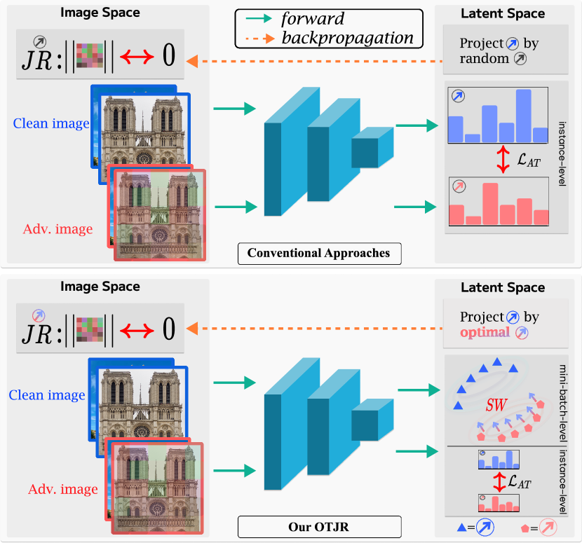
Figure 1. Illustration of (top) two popular approaches to boost a model’s robustness: Adversarial Training (AT) vs. Jacobian regularization (JR), and (bottom) our OTJR method. Jacobian regularization tries to silence the Jacobian matrix at the input end. The AT adjusts the distribution of perturbed samples at the output end. In conventional approach, Jacobian regularization backpropagates through random projections, whereas the AT via a loss function. Our proposed OTJR  bridges AT and Jacobian regularization on framework by the optimal transport theory (Sliced Wasserstein distance).

Deep Neural Networks (DNNs) have established themselves as the de facto method for tackling challenging real-world machine learning problems. Their applications cover a broad range of domains, such as image classification, object detection, and recommendation systems. Nevertheless, recent research has revealed DNNs’ severe vulnerability to adversarial examples  (Christian et al., 2013; Ian et al., 2014), particularly in computer vision tasks. Small imperceptible perturbations added to the image can easily deceive the neural networks into making incorrect predictions with high confidence. Moreover, this unanticipated phenomenon raises social concerns about DNNs’ safety and trustworthiness, as they can be abused to attack many sophisticated and practical machine learning systems putting human lives into danger, such as in autonomous car (Deng et al., 2020) or medical systems  (Ma et al., 2021; Bortsova et al., 2021).

Meanwhile, there are numerous studies that devote their efforts to enhance the robustness of various models against adversarial examples. Among the existing defenses, adversarial training (AT) (Ian et al., 2014; Madry et al., 2018) and Jacobian regularization (JR) (Jakubovitz and Giryes, 2018; Hoffman et al., 2019) are the two most predominant and popular defense approaches . In AT, small perturbations are added to a clean image in its neighbor of $L_{p}$ norm ball to generate adversarial samples. Thus, an adversarially trained model can force itself to focus more on the most relevant image’s pixels. On the other hand, the second approach, Jacobian regularization, mitigates the effect of the perturbation to the model’s decision boundary by suppressing its gradients. However, AT and Jacobian regularization have not been directly compared in both theoretical and empirical settings.

In this work, we embark on a dual-path exploration, offering both theoretical and empirical comparisons between AT and Jacobian regularization. Our objective is to deepen our comprehension of the adversarial robustness inherent to DNN models and subsequently enhance their defensive capability. While a myriad of prior research has spotlighted defense, they predominantly adopt either an empirical or theoretical lens, rarely both. To bridge this gap, we introduce an innovative approach, integrating both Jacobian regularization and AT. This fusion seeks to augment the adversarial robustness and defensive efficacy of a model, as elucidated in Fig. 1.

For AT, a plethora of studies have been proposed, presenting unique strategies to encourage the learning of robust classifiers. (Zhang et al., 2020, 2019; Rony et al., 2019; Kannan et al., 2018; Madry et al., 2018). Notably, Sinkhorn Adversarial Training (SAT) (Bouniot et al., 2021) resonates with our methodology, particularly in its objective to bridge the distributional gap between clean and adversarial samples using optimal transport theory. However, the pillar of their algorithms mainly relies on the Sinkhorn algorithm (Cuturi, 2013) to utilize the space discretization property (Vialard, 2019). Therefore, their approach has several limitations in terms of handling high-dimensional data (Meng et al., 2019; Petrovich et al., 2020). Particularly, the Sinkhorn algorithm blurs the transport plan by adding an entropic penalty to ensure the optimization’s convexity. The entropic penalty encourages the randomness of the transportation map. However, in high-dimensional spaces, such randomness reduces the deterministic movement plan of one sample, causing ambiguity. As a result, when training defense models on a large scale dataset, SAT results in a slow convergence rate, which is unjustifiable due to the introduction of additional training epochs with distinct learning schedules (Pang et al., 2020).

To address the outlined challenges, we present our pioneering method, Optimal Transport with Jacobian Regularization, denoted as  OTJR, designed explicitly to bolster defenses against adversarial intrusions. We leverage the Sliced Wasserstein (SW) distance, which is more efficient for AT in high dimensional space with a faster convergence rate. In addition, the SW distance provides us with other advantages due to optimal latent trajectories of adversarial samples in the embedding space, which is critical for designing an effective defense. We further integrate the input-output Jacobian regularization by substituting its random projections with the optimal trajectories and constructing the optimal Jacobian regularization. Our main contributions are summarized as follows:

(1) Comprehensive Theoretical and Empirical Examination. Our research delves deep into the theoretical underpinnings of adversarial robustness, emphasizing the intricacies of AT and Jacobian Regularization. Distinctively, we pioneer a simultaneous theoretical and empirical analysis, offering an incisive, comparative exploration. This endeavor serves to elucidate the differential impacts that each methodology has on the design and efficacy of defensive DNNs.

(2) Innovative Utilization of the Sliced Wasserstein (SW) Distance. Charting new territory, we introduce the integration of the SW distance within our AT paradigm, denoted as OTJR. This innovation promises a marked acceleration in the training convergence, setting it apart from extant methodologies. Harnessing the prowess of the SW distance, we discern the optimal trajectories for adversarial samples within the latent space. Subsequently, we weave these optimal vectors into the framework of Jacobian Regularization, augmenting the resilience of DNNs by expanding their decision boundaries.

(3) Rigorous Evaluation against White- and Black-box Attacks. Our exhaustive experimental assessments underscore the superiority of our methodology. Pitted against renowned state-of-the-art defense strategies, our approach consistently emerges preeminent, underscoring the potency of enhancing Jacobian Regularization within the AT spectrum as a formidable defensive arsenal.

2. Comparisons between AT and JR

2.1. Theoretical Preliminaries

Let a function $f$ represent a deep neural network (DNN), which is parameterized by $\theta$, and $x\in\mathbb{R}^{I}$ be a clean input image. Its corresponding output vector is $z=f(x)\in\mathbb{R}^{C}$, where $z_{c}$ is proportional to the likelihood that $x$ is in the $c$-th class. Also, let $\tilde{x}=x+\epsilon$ be an adversarial sample of $x$ generated by adding a small perturbation vector $\epsilon\in\mathbb{R}^{I}$. Then, the Taylor expansion of the mapped feature of the adversarial sample with respect to $\epsilon$ is derived as follows:

$$\tilde{z}=f(x+\epsilon) =f(x)+J(x)\epsilon+O(\epsilon^{2})$$

(1) $$\simeq z+J(x)\epsilon,$$

(2) $$||\tilde{z}-z||_{q}\simeq||J(x)\epsilon||_{q}.$$

Table 1. Training objectives of the popular AT frameworks, where $\mathbb{S}$ denotes the softmax function.

AT Framework	Training Objective
TRADES	$\mathcal{L}_{\mathcal{XE}}(\mathbb{S}(z),y)+\lambda\mathcal{L}_{\mathcal{XE}}(\mathbb{S}(\tilde{z}),\mathbb{S}(z))$
PGD-AT	$\mathcal{L}_{\mathcal{XE}}(\mathbb{S}(\tilde{z}),y)$
ALP	$\alpha\mathcal{L}_{\mathcal{XE}}(\mathbb{S}(\tilde{z}),y)+(1-\alpha)\mathcal{L}_{\mathcal{XE}}(\mathbb{S}(\tilde{z}),y)+\lambda||\tilde{z}-z||_{2}$

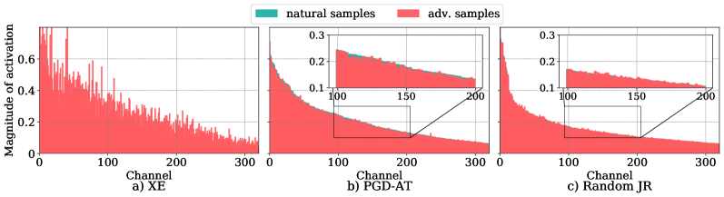
Figure 2. The magnitude of activation at the penultimate layer for models trained with $\mathcal{XE}$ loss, PGD-AT adversarial training, and the input-output Jacobian regularization. The channels in the X-axis are sorted in descending order of the clean samples’ magnitude.

Precisely, Eq. 2 is a basis to derive two primary schools of approaches, AT vs. Jacobian regularization, for mitigating adversarial perturbations and boosting the model robustness. In particular, each side of  Eq. 2 targets the following two objectives, to improve the robustness:

1) Aligning adversarial representation (AT). Minimizing the left-hand side of Eq. 2 is to push the likelihood of an adversarial sample $\tilde{x}$ close to that of a clean sample $x$. For instance, the Kullback-Leibler divergence between two likelihoods is a popular AT framework such as TRADES (Zhang et al., 2019). More broadly, the likelihood differences can include the cross-entropy ($\mathcal{XE}$) loss of adversarial samples such as ALP (Kannan et al., 2018), PGD-AT (Madry et al., 2018), or FreeAT (Shafahi et al., 2019). These well-known AT frameworks are summarized in Table 1, to explain their core learning objective.

2) Regularizing input-output Jacobian matrix (JR). Regularizing the right-hand side of Eq. 2, which is independent of $\tilde{x}$, suppresses the spectrum of the input-output Jacobian matrix $J(x)$. Thus, the model becomes more stable with respect to input perturbation, as it was theoretically and empirically demonstrated in a line of recent research (Jakubovitz and Giryes, 2018; Hoffman et al., 2019; Co et al., 2021). Particularly, by observing $||J(x)\epsilon||_{q}\leq||J(x)||_{F}||\epsilon||$, one can instead minimize the square of the Frobenius norm of the Jacobian matrix, which can be estimated as follows (Hoffman et al., 2019):

(3) $$||J(x)||_{F}^{2}=C\mathbb{E}_{\hat{v}\sim\mathcal{S}^{C-1}}\left[||\hat{v}\cdot J||^{2}\right],$$

where $\hat{v}$ is an uniform random vector drawn from a C-dimensional unit sphere $\mathcal{S}^{C-1}$. Using Monte Carlo method to approximate the integration of $\hat{v}$ over the unit sphere, Eq. 3 can be rewritten as:

(4) $$||J(x)||_{F}^{2}=\frac{1}{n_{\text{proj}}}\sum_{i=1}^{n_{\text{proj}}}\left[\frac{\partial(\hat{v}_{i}\cdot z)}{\partial x}\right]^{2}.$$

Considering a large number of samples in a mini-batch, $n_{\text{proj}}$ is usually set to $1$ for the efficient computation. Hence, the Jacobian regularization is expressed as follows:

(5) $$||J(x)||_{F}^{2}\simeq\left[\frac{\partial(\hat{v}\cdot z)}{\partial x}\right]^{2},\hat{v}\sim\mathcal{S}^{C-1}.$$

Summary. As shown above, each approach takes different direction to tackle adversarial perturbations. While AT targets aligning the likelihoods at the output end, Jacobian regularization forces the norm of the Jacobian matrix at the input to zero, as also pictorially described in Fig. 1. However, their distinct effects on the robustness of a DNN have not been fully compared and analyzed so far.

2.2. Empirical Analysis

We also conduct an experimental analysis to ascertain and characterize the distinct effects of the two approaches (AT vs. Jacobian regularization) on a defense DNN when it is trained with each of the objectives. We use wide residual network WRN34 as the preliminary baseline architecture on CIFAR-10 dataset and apply two canonical frameworks: PGD-AT (Madry et al., 2018) and input-output Jacobian regularization (Hoffman et al., 2019) to enhance the model’s robustness. Details of training settings are provided in the experiment section.

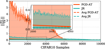
Figure 3. Magnitude of $||\nabla_{\tilde{x}}\mathcal{L}_{\mathcal{XE}}||_{1}$ at the input layer for a model trained with PGD-AT and Jacobian regularization. Red and green-filled areas range from min. to max. values of each sample.

Output and input sides. We measure the magnitude of channel-wise activation to characterize the connection between adversarial defense methods and the penultimate layer’s activation (Bai et al., 2021). Figure 2 provides the average magnitude of activations of clean vs. adversarial samples created by PGD-20 attacks (Madry et al., 2018). As shown, not only AT (Bai et al., 2021), but also Jacobian regularization can effectively suppress the magnitude of the activation. Moreover, the Jacobian regularization typically achieves the lower magnitude value of the activation compared to that of PGD-AT. This observation serves as a clear counter-example to earlier results from  Bai et al.(Bai et al., 2021), where they claim that adversarial robustness can be generally achieved via channel-wise activation suppressing. As such, it is worth noting that while a more effective defense strategy can produce lower activation, the inverse is not always true. In addition, Fig. 3 represents the average gradient of $\mathcal{XE}$ loss with respect to the adversarial samples, at the input layer. This demonstrates that the model trained with Jacobian regularization suppresses input gradients more effectively than a typical AT framework, i.e., PGD-AT. In other words, when a defensive model is abused to generate adversarial samples, pre-training with Jacobian regularization can reduce the severity of perturbations, hindering the adversary’s target.

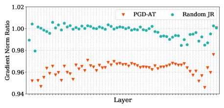
Figure 4. Ratios of $\mathbb{E}(||\nabla_{\theta_{i}}\mathcal{L}(\tilde{x})||/||\nabla_{\theta_{i}}\mathcal{L}({x})||)$ w.r.t. the model’s parameters $\theta_{i}$ on CIFAR-10. The lower the ratios are, the more emphasis the model puts on perturbations.

Layer-by-layer basis. We further provide Fig. 4 to depict the gradients of models trained with PGD-AT, and Jacobin regularization, respectively. Particularly, we compute the norm ratios of the loss gradient on the adversarial sample to the loss gradient on the clean samples for each layer of the model. As we can observe, the model trained with the Jacobian regularization produces higher ratio values, meaning it puts less emphasis on adversarial samples due to its agnostic defense mechanism. Meanwhile, most of the ratio values at the middle layers from Jacobian training vary around 1.This is explained by the regularization applied to its first derivatives. In summary, we can also empirically conclude that the Jacobian regularization tends to silence the gradient of the model from output to input layers. Therefore, it agnostically stabilizes the model under the changes of input samples, and produces low-magnitude adversarial perturbations, when the model is attacked. In contrast, by learning the meaningful pixels from input images, AT adjusts the model’s parameters at every layer in such a way to reduce the impacts of adversarial perturbation on the model’s outputs.

Our motivation. As elucidated by Hoffman et al.(Hoffman et al., 2019), the computational overhead introduced by training models with Jacobian regularization is marginal compared to standard training regimes. Therefore, a combination of AT and Jacobian regularization becomes an appealing approach for the adversarial robustness of a model. Furthermore, taking advantages from both approaches can effectively render a classifier to suppress the perturbation and adaptively learn crucial features from both clean and adversarial samples. However, merely adding both approaches together into the training loss is not the best option. Indeed it is insufficient, since the adversarial representations in the latent space can contain meaningful information for the Jacobian regularization, which we will discuss more in the next section.

Hence, in this work, we propose a novel optimization framework, OTJR, to leverage the movement direction information of adversarial samples in the latent space and optimize the Jacobian regularization. In this fashion, we can successfully establish a relationship and balance between silencing input’s gradients and aligning output distributions, and significantly improve the overall model’s robustness. Additionally, recent studies proposed approaches utilizing a surrogate model (Wu et al., 2020) or teacher-student framework (Cui et al., 2021) during training. Yet, while these methods improve the model’s robustness, they also rely on previous training losses (such as TRADE or PGD). And, they introduce additional computation for the AT, which are so far well-known for their slow training speed and computational overhead. In our experiment, we show that our novel training loss can be compatible with these frameworks and further improve the model’s robustness by a significant margin compared to prior losses.

3. Our Approach

Our approach explores the Sliced Wasserstein distance in order to push the adversarial distribution closer to the natural distribution with a faster convergence rate. Next, the Sliced Wasserstein distance results in optimal movement directions to sufficiently minimize the spectrum of input-output Jacobian matrix.

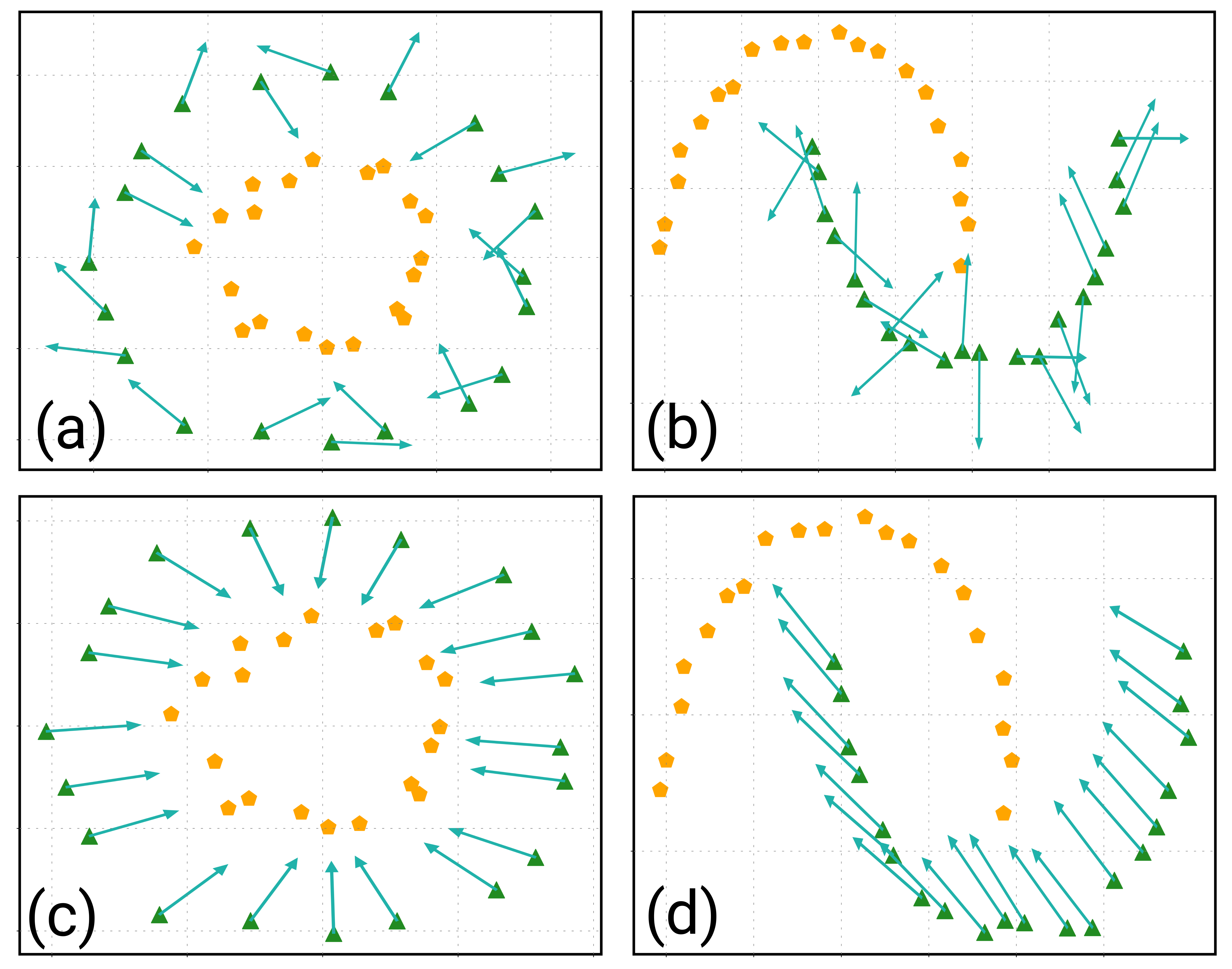
Figure 5. Illustration of optimal latent trajectories. Top row ((a) & (b)): Random movement directions (green arrows), which is non-informative, uniformly sampled from two-dimensional unit sphere $\mathcal{S}^{1}$. Bottom row ((c) & (d)): The optimal trajectories from the SW distance between source distribution (green) and target distribution (orange) obtained from  Eq. 11.

Table 2. Classification accuracy (% ) under white-box, black-box attacks and AutoAttack. Different defense methods trained on CIFAR-10 and CIFAR-100 datasets using WRN34 in 100 epochs, except that SAT⁴⁰⁰ was trained in 400 epochs. Each experiment was conducted three times to ensure reliability. Standard deviations are denoted with subscripts. Numbers underlined represent the greatest reduction in performance on clean images to trade-off for robustness. Best performances are highlighted in bold.

Dataset	Defense	Clean	PGD20	PGD100	$L_{2}$-PGD	MIM	FGSM	CW	FAB	Square	SimBa	AutoAtt
CIFAR-10	TRADES	84.71.15	54.23.07	53.91.11	61.04.21	54.13.11	60.46.15	53.17.22	53.65.39	62.25.26	70.66.52	52.06.15
	ALP	86.63.23	46.99.25	46.48.25	55.69.33	46.88.23	58.14.21	47.50.30	55.61.27	59.26.28	68.28.31	46.28.25
	PGD-AT	86.54.20	46.67.11	46.23.12	55.93.10	46.66.09	56.83.23	47.56.15	48.39.22	58.92.12	68.66.14	45.77.07
	SAT	83.19.33	53.52.15	53.23.23	60.37.06	52.461.34	60.36.13	52.15.20	52.54.36	61.50.19	69.70.29	50.73.20
	Random JR	84.99.14	22.67.15	21.89.14	60.98.19	22.49.18	32.99.21	22.00.06	21.74.11	45.86.20	71.20.31	20.54.14
	SW	84.26.80	54.51.33	54.20.37	61.08.12	54.46.27	61.32.12	53.78.05	54.90.29	62.95.43	70.74.65	51.97.06
	OTJR (ours)	84.01.53	55.38.29	55.08.36	63.87.09	55.31.29	61.03.18	54.09.12	54.17.07	63.11.21	72.04.68	52.57.12
CIFAR-100	TRADES	57.46.16	30.42.05	30.36.09	35.85.10	30.37.08	33.04.16	27.97.13	27.93.15	33.70.06	44.28.14	27.15.09
	ALP	60.61.05	26.23.18	25.87.17	33.75.09	26.14.07	31.40.08	25.78.22	25.69.15	33.09.15	43.25.22	24.57.22
	PGD-AT	59.77.21	24.05.03	23.74.03	31.41.16	24.01.06	29.21.18	24.67.04	24.47.06	31.47.11	41.15.21	23.28.01
	SAT400	53.61.52	26.63.14	26.42.16	32.34.25	26.57.19	31.04.21	25.22.06	26.63.11	31.32.34	39.64.90	24.32.05
	Random JR	66.58.17	9.41.44	8.87.42	37.79.31	9.27.49	16.38.33	10.27.45	9.26.23	23.53.15	48.86.55	8.10.57
	SW	57.69.28	26.01.16	25.82.24	31.37.17	25.97.18	30.78.34	25.48.23	26.11.07	31.34.26	40.68.43	24.35.29
	OTJR (ours)	58.20.13	32.11.21	32.01.18	43.13.12	32.07.19	34.26.30	29.71.06	29.24.08	36.27.05	49.92.23	28.36.10

3.1. Sliced Wasserstein Distance

The p-Wasserstein distance between two probability distributions $\mu$ and $\nu$ (Villani, 2008) in a general d-dimensional space $\Omega$, to search for an optimal transportation cost between $\mu$ and $\nu$, is defined as follows:

(6) $$\small W_{p}(P_{\mu},P_{\nu})=\Big{(}\inf_{\pi\in\Pi(\mu,\nu)}\int_{\Omega\times\Omega}\psi(x,y)^{p}d\pi(x,y)\Big{)}^{1/p},$$

where $\psi:\Omega\times\Omega\rightarrow\mathbb{R}^{+}$ is a transportation cost function, and $\Pi(\mu,\nu)$ is a collection of all possible transportation plans. The Sliced p-Wasserstein distance ($SW_{p}$), which is inspired by the $W_{p}$ in one-dimensional, calculates the p-Wasserstein distance by projecting $\mu$ and $\nu$ onto multiple one-dimensional marginal distributions using Radon transform (Helgason, 2010). The $SW_{p}$ is defined as follows:

(7) $$\small SW_{p}(\mu,\nu)=\int_{\mathcal{S}^{d-1}}W_{p}(\mathcal{R}_{(t,\hat{v})}\mu,\mathcal{R}_{(t,\hat{v})}\nu)d\hat{v},$$

where $\mathcal{R}_{(t,\hat{v})}\mu$ is the Radon transform as follows:

(8) $$\small\mathcal{R}_{(t,\hat{v})}\mu=\int_{\Omega}\mu(x)\sigma(t-\langle\hat{v},x\rangle)dx,\forall\hat{v}\in\mathcal{S}^{d-1},\forall t\in\mathbb{R},$$

where $\langle\cdot,\cdot\rangle$ denote the Euclidean inner product, and $\sigma$ is the Dirac delta function.

Next, let $\mathcal{B}$ denote the size of a mini-batch of samples, and $C$ denote the number of classes. To calculate the transportation cost between adversarial samples’ representations $\mu:=\{\tilde{z}_{i}\}_{\mathcal{B}}$ and the corresponding original samples’ representations $\nu:=\{z_{i}\}_{\mathcal{B}}$, the integration of $\hat{v}$ over the unit sphere $\mathcal{S}^{C-1}$ is approximated via Monte Carlo method with $K$ uniformly sampled random vector $\hat{v}_{i}\in\mathcal{S}^{C-1}$. In particular, $\mathcal{R}_{(t,\hat{v})}\mu$ and $\mathcal{R}_{(t,\hat{v})}\nu$ are sorted in ascending order using two permutation operators $\tau_{1}$ and $\tau_{2}$, respectively, and the approximation of Sliced 1-Wasserstein is expressed as follows:

(9) $$\small SW(\mu,\nu)\simeq\sum_{k=1}^{K}\psi\left(\tau_{1}\circ\mathcal{R}_{(t,\hat{v}_{k})}\mu,\tau_{2}\circ\mathcal{R}_{(t,\hat{v}_{k})}\nu\right).$$

3.2. Optimal Latent Trajectory

Using Eq. 9, we can straightforwardly compute the trajectory of each $\tilde{z}_{i}$ in the latent space $\mathbb{R}^{C}$ in order to minimize the $SW(\mu,\nu)$. We refer to the directions of these movements as optimal latent trajectories, because the SW distance produces the lowest transportation cost between the source and target distributions. Particularly, let the trajectories of $\{\tilde{z}_{i}\}_{\mathcal{B}}$ in each single projection $\hat{v}_{k}$ be:

(10) $$m_{k}=(\tau_{1}^{-1}\circ\tau_{2}\circ\mathcal{R}_{(t,\hat{v}_{k})}\nu-\mathcal{R}_{(t,\hat{v}_{k})}\mu)\otimes\hat{v}_{k},$$

where $\otimes$ denotes the outer product. Then, the overall optimal trajectory direction of each $\tilde{z}_{i}$ is expressed as follows:

(11) $$\sigma_{i}=\frac{\sum_{k=1}^{K}m_{k,i}}{||\sum_{k=1}^{K}m_{k,i}||_{2}}.$$

A demonstrative example is provided in Figure 5 to illustrate the concept of optimal trajectories. This example highlights the trajectory direction of an adversarial sample, denoted as $\tilde{x}$, within the latent space. In particular, this direction is significant, as it represents the most sensitive axis of perturbation for $x$ when exposed to adversarial interference. To address this, our approach diverges from the traditional method of random projection, as previously proposed by Hoffman et al. (2019) (Hoffman et al., 2019). Instead, we propose to regularize the Jacobian matrix of $x$ specifically along this identified optimal trajectory. Utilizing Eq. 5, we are able to reformulate the input-output Jacobian regularization, incorporating these strategically derived projections for each sample. The formula for this new regularization approach is presented below:

(12) $$||J(x_{i}|\sigma_{i})||_{F}^{2}\simeq\left[\frac{\partial(\sigma_{i}\cdot z_{i})}{\partial x_{i}}\right]^{2}.$$

Then, our overall loss function for a batch of samples $\{(x_{i},y_{i})\}_{\mathcal{B}}$ is expressed in the following way:

(13) $$\mathcal{L}=\sum^{\mathcal{B}}_{i=1}\left(\mathcal{L_{\text{AT}}}(\tilde{x_{i}},y_{i})+\lambda_{J}||J(x_{i}|\sigma_{i})||_{F}^{2}\right)+\lambda_{SW}SW(\mu,\nu),$$

where $\mathcal{L}_{\text{AT}}$, unless stated otherwise, is cross-entropy loss of adversarial samples. In practice, sampling $K$ uniform vectors $\hat{v}_{k}$ can be performed simultaneously thanks to deep learning libraries. Then, the calculation of random projections and optimal trajectory steps can be vectorized and performed simultaneously.

4. Experimental Results

4.1. Experiment Settings

We employ WideResNet34-10 (Zagoruyko and Komodakis, 2016) as our backbone architecture on two datasets CIFAR-10 and CIFAR-100 (Krizhevsky et al., 2009). The model are trained for 100 epochs with the momentum SGD (Qian, 1999) optimizer, whereas its initial learning rate is set to 0.1 and decayed by $10$ at $75^{th}$ and $90^{th}$ epoch, respectively. Adversarial samples in the training phase are generated by $L_{\infty}$-PGD (Madry et al., 2018) in 10 iterations with the maximal perturbation $\epsilon=8/255$ and the perturbation step size $\eta=2/255$. For a fair comparison with different approaches (Pang et al., 2020), we use the above settings throughout our experiments without early stopping or modifying models’ architecture, and report their performances on the last epoch. For our OTJR based defense models, we use the following hyper-parameter settings: $\{K=32,\lambda_{J}=0.002,\lambda_{SW}=64\}$ and $\{K=128,\lambda_{J}=0.001,\lambda_{SW}=64\}$ for CIFAR-10 and CIFAR-100, respectively. An ablation study of the hyper-parameters’ impact on model performance is provided in Sec. C in the Appendix. In addition, we perform the basic sanity tests (Carlini et al., 2019) in Sec.4.5.1 to ensure that our proposed OTJR does not rely on gradient obfuscation. Overall, we compare our method with four different recent SOTA AT frameworks: TRADES (Zhang et al., 2019), ALP (Kannan et al., 2018), PGD-AT (Madry et al., 2018), and SAT (Bouniot et al., 2021). The experiments are conducted on one GeForce RTX 3090 24GB GPU with Intel Xeon Gold 6230R CPU @ 2.10GHz.

Table 3. Online fool rate (%) (Mladenovic et al., 2021) of various defense models with our downloaded  CIFAR-10-WEB  and  CIFAR-100-WEB  datasets.

Defense	CIFAR-10-WEB			CIFAR-100-WEB
	$k=100$	$k=200$	$k=500$	$k=100$	$k=200$	$k=500$
TRADES	78.13.0	75.62.1	46.91.4	84.73.4	85.52.2	84.91.5
ALP	78.62.9	77.12.0	49.11.4	85.14.6	85.62.3	85.31.7
PGD-AT	79.22.6	79.82.1	51.41.6	84.93.6	86.22.9	86.30.9
SAT	77.75.4	72.83.2	48.62.1	86.92.6	87.2 1.8	87.20.6
Random JR	82.33.9	82.52.8	63.71.3	90.52.9	90.11.7	90.01.4
SW	77.64.2	72.02.3	46.01.6	83.94.0	85.52.6	85.51.2
OTJR	74.04.3	71.33.1	46.01.9	84.93.8	84.62.5	84.11.4

Table 4. Classification accuracy (%) from defense losses integrated AWP, LBGAT, and UDR, respectively, on WRN34 with CIFAR-100. $\ast$ indicates baseline results obtained from downloaded models. $\dagger$ indicates re-running original paper settings.

Defense	AWP∗		LBGAT∗		UDR†
	Clean	AutoAtt	Clean	AutoAtt	Clean	AutoAtt
TRADES	60.17	28.80	60.43	29.34	68.04	47.87
OTJR	60.55	29.79	62.15	29.64	68.31	49.34

Table 5. Classification accuracy (%) of PreActResNet18 with Tiny-IMAGENET dataset, under white- and black-box attacks.

Defense	Clean	MIM	CW	FAB	Square	AutoAtt	Avg.
TRADES	35.91${}_{\text{.10}}$	11.82${}_{\text{.08}}$	8.92${}_{\text{.13}}$	10.88${}_{\text{.24}}$	15.86${}_{\text{.04}}$	8.28${}_{\text{.09}}$	11.15${}_{\text{3.00}}$
ALP	39.69${}_{\text{.37}}$	8.13${}_{\text{.06}}$	7.66${}_{\text{.08}}$	9.92${}_{\text{.16}}$	15.98${}_{\text{.34}}$	6.48${}_{\text{.10}}$	9.63${}_{\text{3.75}}$
PGD	33.81${}_{\text{.22}}$	11.49${}_{\text{.33}}$	10.14${}_{\text{.24}}$	11.29${}_{\text{.32}}$	16.20${}_{\text{.43}}$	8.98${}_{\text{.16}}$	11.60${}_{\text{2.77}}$
SAT400	Not converge						-
Random JR	47.65${}_{\text{.19}}$	0.29${}_{\text{.02}}$	0.44${}_{\text{.04}}$	3.79${}_{\text{.13}}$	5.87${}_{\text{.03}}$	0.19${}_{\text{.01}}$	2.12${}_{\text{2.59}}$
SW	37.05${}_{\text{.09}}$	12.43${}_{\text{.21}}$	9.35${}_{\text{.19}}$	11.19${}_{\text{.14}}$	16.77${}_{\text{.31}}$	8.72${}_{\text{.14}}$	11.19${}_{\text{3.20}}$
OTJR	37.97${}_{\text{.11}}$	12.57${}_{\text{.08}}$	9.55${}_{\text{.04}}$	11.30${}_{\text{.09}}$	17.33${}_{\text{.12}}$	8.91${}_{\text{.08}}$	11.97${}_{\text{3.34}}$

4.2. Popular Adversarial Attacks

Follow Zhang et al., we assess defense methods against a wide range white-box attacks (20 iterations): FGSM (Ian et al., 2014), PGD (Madry et al., 2018), MIM (Dong et al., 2018), CW_∞ (Carlini and Wagner, 2017), DeepFool (Moosavi-Dezfooli et al., 2016), and FAB (Croce and Hein, 2020a); and black-box attacks (1000 iterations): Square (Andriushchenko et al., 2020) and Simba (Guo et al., 2019). We use the same parameters as Rice et al. for our experiments: for the $L_{\infty}$ threat model, the values of epsilon and step size are $8/255$ and $2/255$ for CIFAR-10 and CIFAR-100, respectively. For the $L_{2}$ threat model, the values of epsilon and step size are 128/255 and 15/255 for all datasets. Additionally, we include AutoAttack (Croce and Hein, 2020b) which is a reliable adversarial evaluation framework and an ensemble of four distinct attacks: APGD-CE, APGD-DLR (Croce and Hein, 2020b), FAB (Croce and Hein, 2020a), and Square (Andriushchenko et al., 2020). The results of this experiment are presented in Table 2, where the best results are highlighted in bold. Evidently, our proposed OTJR method demonstrates its superior performance across different attack paradigms. The improvement is considerable on AutoAttack, by more than $0.51\%$ and $1.21\%$ on average compared to other methods on CIFAR-10 and CIFAR-100, respectively. In addition, we include two primary components of our proposed OTJR, i.e., SW and random JR in Table 2. While the random JR, as expected, is highly vulnerable to most of the white-box attacks due to its adversarial-agnostic defense strategy, the SW approach is on par with other AT methods.

4.3. Online Adversarial Attacks

In order to validate the applicability of our defense model in real-world systems, we employ the stochastic virtual method (Mladenovic et al., 2021). This method is designed as an online attack algorithm with a transiency property; that is, an attacker makes an irrevocable decision regarding whether to initiate an attack or not.

For our experiment, we curate a dataset by downloading 1,000 images and categorizing them into 10 distinct classes, mirroring the structure of the CIFAR-10 dataset. We refer to this new subset as CIFAR-10-WEB. In a similar vein, we assemble a CIFAR-100-WEB  dataset comprising 5,000 images on the Internet, distributed across 100 classes analogous to the CIFAR-100 dataset. To ensure the reliability of our findings, we replicate the experiment ten times. The outcomes of these trials are detailed in Table 3. Notably, our novel system, OTJR, persistently showcases the most minimal fooling rate in comparison to other methods in the k-secretary settings (Mladenovic et al., 2021), underscoring its robustness for real-world applications.

4.4. Compatibility with Different Frameworks and Datasets

4.4.1. Frameworks with surrogate models and relaxed perturbations

AWP (Wu et al., 2020) and LBGAT (Cui et al., 2021) are two SOTA benchmarks boosting adversarial robustness using surrogate models during training, albeit rather computationally expensive. Furthermore, they utilized existing AT losses, such as TRADES. We integrate our proposed optimization loss into AWP and LBGAT, respectively. Additionally, we also include the results of UDR (Bui et al., 2022) that used for creating relaxed perturbed noises upon its entire distribution. We selected TRADES as the best existing loss function that was deployed with these frameworks and experimented with CIFAR-100-WRN34 for comparison. For consistent comparison, we use TRADES loss as our $\mathcal{L}_{\text{AT}}$ in Eq. 13. As shown in Table 4, our OTJR is compatible with the three frameworks and surpasses the baseline performance by a significant margin.

4.4.2. Large scale dataset

We conducted further experiments on Tiny-IMAGENET with PreactResnet18, comparing our method against competitive AT methods under most challenging attacks, including MIM, CW, FAB, Square, and AutoAttack, in Table 5. All defensive methods are trained in 150 epochs with same settings as in Sec. 4.1. We note that SAT unable to converge within 400 epochs. As observed, our method not only sustains competitive performance on clean sample but also displays superior robustness against adversarial perturbations, while the second best robust model, PGD, has to sacrifice substantially its clean accuracy compared to ours (33.81% vs. 37.97%). In addition, this experiment illustrates that our proposed approach does not hinder the convergence process, unlike certain alternative optimum transport methods such as SAT, when applied to datasets of significant size.

Table 6. Basic sanity tests for our  OTJR  method with white-box PGD attack.

Number of step
Clean	1	10	20	40	50
84.01${}_{\text{.53}}$	78.86${}_{\text{.69}}$	56.26${}_{\text{.24}}$	55.38${}_{\text{.29}}$	55.1${}_{\text{.40}}$	55.08${}_{\text{.40}}$
Perturbation budget $\epsilon$ w/ PGD-20
Clean	8/255	16/255	24/255	64/255	128/255
84.01${}_{\text{.53}}$	55.38${}_{\text{.29}}$	24.57${}_{\text{1.00}}$	9.66${}_{\text{.54}}$	0.57${}_{\text{.01}}$	0.00${}_{\text{.01}}$

4.5. Ablation Studies and Discussions

4.5.1. Sanity Tests

The phenomenon of gradient obfuscation arises, when a defense method is tailored such that its gradients prove ineffective for generating adversarial samples (Athalye et al., 2018). However, the method designed in that manner can be an incomplete defense to adversarial examples (Athalye et al., 2018). Adhering to guidelines from (Carlini et al., 2019), we evaluate our pre-trained model on CIFAR10 with WRN34 to affirm our proposed  OTJR  does not lean on gradient obfuscation. As detailed in Table 6, iterative attacks are strictly more powerful than single-step attacks, whereas when increasing perturbation budget $\epsilon$ can also raise attack successful rate. Finally, the PGD attack attains a 100% success rate when $\epsilon=128/255$.

4.5.2. Loss’s derivative.

In continuation with our preliminary analysis, we highlight the disparities in defense model gradients across layers between our OTJR and SAT. Throughout intermediate layers in an attacked model, both frameworks provide stable ratios between perturbed and clean sample’s gradients as shown in Fig. 6. It is worth noting that the gradients are derived on unobserved samples in the test set. In the forward path, our OTJR adeptly equilibrates gradients of adversarial and clean samples, with the majority of layers presenting ratio values approximating 1. Moreover, in the backward path, since the victim model’s gradients are deployed to generate more perturbations, our OTJR  model achieves better robustness when it can produce smaller gradients w.r.t. its inputs.

Figure 6. Average gradient norm ratios between adversarial and clean samples. The ratios of $\mathbb{E}(||\nabla_{\theta_{i}}\mathcal{L}(\tilde{x})||/||\nabla_{\theta_{i}}\mathcal{L}({x})||)$ with respect to the model’s parameters $\theta_{i}$ on CIFAR-10 dataset.

Table 7. Average derivative of $\mathcal{XE}$ loss w.r.t input ${x}$ at the pixel level after various PGD iterations. The lower the derivative is, the less perturbed the adversarial samples are when the model is abused. Best results are in bold.

Method	$\mathbb{E}(||\nabla_{{x}}\mathcal{L})||_{1})$
	Clean	$PGD^{1}$	$PGD^{5}$	$PGD^{10}$	$PGD^{15}$	$PGD^{20}$
$\mathcal{XE}$	854$\cdot e^{-4}$	5492$\cdot e^{-4}$	4894$\cdot e^{-4}$	4852$\cdot e^{-4}$	4975$\cdot e^{-4}$	4900$\cdot e^{-4}$
Random JR	105$\cdot e^{-4}$	149$\cdot e^{-4}$	272$\cdot e^{-4}$	335$\cdot e^{-4}$	360$\cdot e^{-4}$	370$\cdot e^{-4}$
PGD	158$\cdot e^{-4}$	232$\cdot e^{-4}$	420$\cdot e^{-4}$	520$\cdot e^{-4}$	568$\cdot e^{-4}$	586$\cdot e^{-4}$
ALP	118$\cdot e^{-4}$	161$\cdot e^{-4}$	249$\cdot e^{-4}$	298$\cdot e^{-4}$	322$\cdot e^{-4}$	332$\cdot e^{-4}$
TRADES	45$\cdot e^{-4}$	53$\cdot e^{-4}$	73$\cdot e^{-4}$	84$\cdot e^{-4}$	89$\cdot e^{-4}$	90$\cdot e^{-4}$
SAT	48$\cdot e^{-4}$	54$\cdot e^{-4}$	65$\cdot e^{-4}$	75$\cdot e^{-4}$	81$\cdot e^{-4}$	84$\cdot e^{-4}$
OTJR  (Ours)	43$\cdot e^{-4}$	48$\cdot e^{-4}$	61$\cdot e^{-4}$	70$\cdot e^{-4}$	73$\cdot e^{-4}$	75$\cdot e^{-4}$

Table 8. Comparison between ours and SAT$+$Random JR on  CIFAR-10 and  CIFAR-100 with WRN34.

Dataset

Defense

Clean

PGD20

PGD100

$L_{2}$-PGD

MIM

FGSM

CW

FAB

Square

SimBa

AutoAtt

CIFAR-10

SAT+JR

83.75${}_{\text{.48}}$

54.15${}_{\text{.17}}$

53.87${}_{\text{.07}}$

62.37${}_{\text{.33}}$

54.12${}_{\text{.16}}$

60.25${}_{\text{.22}}$

52.22${}_{\text{.31}}$

52.63${}_{\text{.53}}$

61.72${}_{\text{.39}}$

71.03${}_{\text{.65}}$

51.15${}_{\text{.37}}$

OTJR (ours)

84.01${}_{\text{.53}}$

55.38${}_{\text{.29}}$

55.08${}_{\text{.36}}$

63.87${}_{\text{.09}}$

55.31${}_{\text{.29}}$

61.03${}_{\text{.18}}$

54.09${}_{\text{.12}}$

54.17${}_{\text{.07}}$

63.11${}_{\text{.21}}$

72.04${}_{\text{.68}}$

52.57${}_{\text{.12}}$

CIFAR-100

SAT+JR400

52.131.55

26.18${}_{\text{.46}}$

25.99${}_{\text{.40}}$

32.64${}_{\text{.90}}$

26.11${}_{\text{.43}}$

30.14${}_{\text{.84}}$

25.10${}_{\text{.47}}$

25.19${}_{\text{.85}}$

30.391.02

39.711.14

23.79${}_{\text{.42}}$

OTJR (ours)

58.20${}_{\text{.13}}$

32.11${}_{\text{.21}}$

32.01${}_{\text{.18}}$

43.13${}_{\text{.12}}$

32.07${}_{\text{.19}}$

34.26${}_{\text{.30}}$

29.71${}_{\text{.06}}$

29.24${}_{\text{.08}}$

36.27${}_{\text{.05}}$

49.92${}_{\text{.23}}$

28.36${}_{\text{.10}}$

Table 9. Accuracy ($\%$) of WRN34 model trained with JR having random projections, and informative projections respectively.

Dataset

Defense

Clean

PGD20

PGD100

$L_{2}$-PGD

MIM

FGSM

CW

FAB

Square

SimBa

AutoAtt

CIFAR-10

Random JR

84.99${}_{\text{.14}}$

22.67${}_{\text{.15}}$

21.89${}_{\text{.14}}$

60.98${}_{\text{.19}}$

22.49${}_{\text{.18}}$

32.99${}_{\text{.21}}$

22.00${}_{\text{.06}}$

21.74${}_{\text{.11}}$

45.86${}_{\text{.20}}$

71.20${}_{\text{.31}}$

20.54${}_{\text{.14}}$

Optimal JR

84.47${}_{\text{.15}}$

24.81${}_{\text{.56}}$

23.97${}_{\text{.48}}$

61.67${}_{\text{.50}}$

24.62${}_{\text{.49}}$

34.22${}_{\text{.50}}$

23.91${}_{\text{.70}}$

24.74${}_{\text{.49}}$

47.18${}_{\text{.54}}$

73.59${}_{\text{.15}}$

22.84${}_{\text{.64}}$

CIFAR-100

Random JR

66.58${}_{\text{.17}}$

9.41${}_{\text{.44}}$

8.87${}_{\text{.42}}$

37.79${}_{\text{.31}}$

9.27${}_{\text{.49}}$

16.38${}_{\text{.33}}$

10.27${}_{\text{.45}}$

9.26${}_{\text{.23}}$

23.53${}_{\text{.15}}$

48.86${}_{\text{.55}}$

8.10${}_{\text{.57}}$

Optimal JR

65.16${}_{\text{.27}}$

10.90${}_{\text{.29}}$

10.32${}_{\text{.35}}$

38.73${}_{\text{.20}}$

10.78${}_{\text{.32}}$

17.30${}_{\text{.29}}$

11.29${}_{\text{.43}}$

10.43${}_{\text{.34}}$

24.23${}_{\text{.41}}$

50.31${}_{\text{.13}}$

9.14${}_{\text{.34}}$

In addition, in Table 7, we present the average magnitude of cross-entropy loss’s derivative w.r.t. the input images from CIFAR-10 dataset with different PGD white-box attack iterations on WRN34. Notably, as the number of attack iterations increases, the perturbation noise induced by the output loss derivatives intensifies. However, our proposed framework consistently exhibits the lowest magnitude across all iterations. This characteristic underscores the superior robustness performance of OTJR.

4.5.3. SW distance vs. Sinkhorn divergence

Bouniot et al. propose the SAT algorithm that deploys Sinkhorn divergence to push the distributions of clean and perturbed samples towards each other (Bouniot et al., 2021). While SAT can achieve comparable results to previous research, its limitations become pronounced in high-dimensional space, i.e., datasets with a large number of classes exhibit slower convergence, as demonstrated in other research (Meng et al., 2019; Petrovich et al., 2020). Our empirical results indicate that SAT struggles to converge within 100 epochs for the CIFAR-100 dataset. Meanwhile, we observed that hyper-parameter settings highly affect the adversarial training (Pang et al., 2020), and the performance improvement by SAT can be partly achieved with additional training epochs. Nevertheless, we still include results from SAT trained in 400 epochs on  CIFAR-100 in (Bouniot et al., 2021).

4.5.4. Our OTJR vs. Naive Combination of SAT & random JR

To discern the impact of Jacobian regularization and distinguish our method from the naive combination of SAT and JR, we report their robustness under wide range of white-box PGD attack in Table 8. The experiments are conducted with  CIFAR-10 and  CIFAR-100 with WRN34. Our optimal approach attains slightly better robustness on small dataset ( CIFAR-10). On the large dataset ( CIFAR-100), however, our  OTJR  achieves significant improvement. This phenomenon is explained by the fact that regularizing the input-output Jacobian matrix increases the difficulty of the SAT algorithm’s convergence, which results in a slower convergence. Therefore, naively combining AT and random Jacobian regularization can restrain the overall optimization process.

4.5.5. Optimal vs. random projections

To verify the efficiency of the optimal Jacobian regularization, WRN34 is trained on  CIFAR-10 using $\mathcal{XE}$ loss with clean samples and the regularization term using Eq. 5 and Eq. 12 respectively, as follow:

(14) $$\mathcal{L}=\sum^{\mathcal{B}}_{i=1}\left(\mathcal{L_{XE}}(x_{i},y_{i})+\lambda_{J}||J(x_{i})||_{F}^{2}\right),$$

where $\lambda_{J}$ is a hyper-parameter to balance the regularization term and $\mathcal{XE}$ loss that is set to 0.02 for this experiment. As we can observe from Table 9, the Jacobian regularized model trained with SW-supported projections consistently achieves higher robustness, compared to the random projections. As shown, our proposed optimal regularization consistently achieves up to 2.5% improvement in accuracy under AuttoAttack compared to the random one.

In addition, we highlight the advantages of optimal Jacobian regularization on decision boundaries in Fig.7. Models trained without this regularizer are notably susceptible to perturbations. However, integrating the Jacobian regularizer augments robustness by broadening the decision boundaries, evidenced by an enlarged black circle. Our optimal Jacobian regularizer further extends the decision boundaries, amplifying model resilience. The rationale behind this enhancement lies in the informative directions showcased in Fig.5, guiding the model to achieve optimal projections within the input-output Jacobian regularization framework.

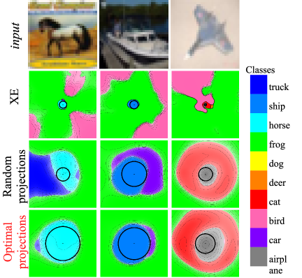
Figure 7. Cross sections of decision boundaries in the input space. 1st row: Sample input images. 2nd row: Model trained without regularization. 3rd row: Model train with Jacobian regularization having random projection. 4th row: Model trained with Jacobian regularization having informative projections. Our optimal JR benefits from the informative directions obtained by SW distance, and thus helps the model to regularize these sensitive direction of clean samples and produce larger decision cells.

5. Conclusion

In the realm of deep learning, which powers a vast array of applications, maintaining the integrity of information is paramount. In this dynamic, our research stands as the inaugural comprehensive exploration into the interplay between Adversarial Training (AT) and Jacobian regularization, especially in bolstering the robustness of Deep Neural Networks (DNNs) against adversarial forays. We show that the AT pays more attention to meaningful input samples’ pixels, whereas the Jacobian regularizer agnostically silences the DNN’s gradients under any perturbation from its output to input layers. Based on these characterizations, we effectively augment the AT framework by integrating input-output Jacobian matrix in order to more effectively improve the DNN’s robustness. Using the optimal transport theory, our work is the first to jointly minimize the difference between the distributions of original and adversarial samples with much faster convergence. Also, the proposed SW distance produces the optimal projections for the Jacobian regularization, which can further increase the decision boundaries of a sample under perturbations, and achieves much higher performance through optimizing the best of both worlds. Our rigorous empirical evaluations, pitted against four state-of-the-art defense mechanisms across both controlled and real-world datasets, underscore the supremacy of our methodology.

Appendix

Appendix A Threat Model and Adversarial Sample

In this section, we summarize essential terminologies of adversarial settings related to our work. We first define a threat model, which consists of a set of assumptions about the adversary. Then, we describe the generation mechanism of adversarial samples in AT frameworks for the threat model defending against adversarial attacks.

A.1. Threat Model

Adversarial perturbation was firstly discovered by Christian et al., and it instantly strikes an array of studies in both adversarial attack and adversarial robustness.  Carlini et al. specifies a threat model for evaluating a defense method including a set of assumptions about the adversary’s goals, capabilities, and knowledge, which are briefly delineated as follows:

• Adversary’s goals could be either simply deceiving a model to make the wrong prediction to any classes from a perturbed input or making the model misclassify a specific class to an intended class. They are known as untargeted and targeted modes, respectively.

• Adversary’s capabilities define reasonable constraints imposed on the attackers. For instance, a $L_{p}$ certified robust model is determined with the worst-case loss function $\mathcal{L}$ for a given perturbation budget $\epsilon$:

  (15) $$\mathbb{E}_{(x,y)\sim\mathcal{D}}\Bigg{[}\max_{\tilde{x}\in{B}_{p}(x,\epsilon)}\mathcal{L}(f(\tilde{x}),y)\Bigg{]},$$

  where ${B}_{p}(x,\epsilon)=\{u\in\mathbb{R}^{\mathcal{I}}:||u-x||_{p}\leq\epsilon\}$.

• Adversary’s knowledge indicates what knowledge of the threat model that an attacker is assumed to have. Typically, white-box and black-box attacks are two most popular scenarios studied. The white-box settings assume that attackers have full knowledge of the model’s parameters and its defensive scheme. In contrast, the black-box settings have varying degrees of access to the model’s parameter or the defense.

Bearing these assumptions about the adversary, we describe how a defense model generates adversarial samples for its training in the following section.

A.2. Adversarial Sample in AT

Among multiple attempts to defend against adversarial perturbed samples, adversarial training (AT) is known as the most successful defense method. In fact, AT is an data-augmenting training method that originates from the work of (Ian et al., 2014), where crafted adversarial samples are created by the fast gradient sign method (FGSM), and mixed into the mini-batch training data. Subsequently, a wide range of studies focus on developing powerful attacks (Kurakin et al., 2016; Dong et al., 2018; Carlini and Wagner, 2017; Croce and Hein, 2020a). Meanwhile, in the opposite direction to the adversarial attack, there are also several attempts to resist against adversarial examples (Kannan et al., 2018; Zhang and Wang, 2019; Shafahi et al., 2019). In general, a defense model is optimized by solving a minimax problem:

(16) $$\min_{\theta}\Big{[}\max_{\tilde{x}\in{B}_{p}(x,\epsilon)}\mathcal{L_{XE}}(\tilde{x},y;\theta)\Big{]},$$

where the inner maximization tries to successfully create perturbation samples subjected to an $\epsilon$-radius ball $B$ around the clean sample $x$ in $L_{p}$ space. The outer minimization tries to adjust the model’s parameters to minimize the loss caused by the inner attacks. Among existing defensive AT, PGD-AT (Madry et al., 2018) becomes the most popular one, in which the inner maximization is approximated by the multi-step projected gradient (PGD) method:

(17) $$\tilde{x}_{t+1}=\Pi_{x}^{\epsilon}(\tilde{x_{t}}+\eta\cdot\text{sgn}(\nabla_{\tilde{x_{t}}}\mathcal{L}(\tilde{x_{t}},y))),$$

where $\Pi_{x}^{\epsilon}$ is an operator that projects its input into the feasible region ${B}_{\infty}(x,\epsilon)$, and $\eta\in\mathbb{R}$ is called step size. The loss function in Eq. 17 can be modulated to derive different variants of generation mechanism for adversarial samples in AT. For example, Zhang et al. (Zhang et al., 2019) utilizes the loss between the likelihood of clean and adversarial samples for updating the adversarial samples. In our work, we use Eq. 17 as our generation mechanism for our AT framework.

Algorithm 1 OTJR: AT with SW and optimal Jacobian regularization

1:DNN $f$ parameterized by $\theta$, training dataset $\mathcal{D}$. Number of projection $K$. Maximum perturbation $\epsilon$, step size $\eta$, number of adversarial iteration $P$. Loss’ hyper-parameters $\lambda_{J}$ and $\lambda_{SW}$. Learning rate $\alpha$ and a mini-batch size of $\mathcal{B}$.

2:while not converged do

3:     for $\{(x_{i},\textrm{ }y_{i})\}_{\mathcal{B}}\in\mathcal{D}$ do

4:         $\nu:=z_{i}=f_{\theta}(x_{i})|_{i=1,..,\mathcal{B}}$ $\triangleright$ forward a batch of clean samples through the model

5:         for iteration $t\leftarrow 1$ to $P$ do

6:              $\tilde{x_{i}}=\Pi_{x}^{\epsilon}(\tilde{x_{i}}+\eta\cdot\text{sgn}(\nabla_{\tilde{x_{i}}}\mathcal{L}(\tilde{x_{i}},y_{i})))|_{i=1,..,\mathcal{B}}$ $\triangleright$ generate adv. samples by $L_{\infty}$-PGD in $P$ iterations

7:         end for

8:         $\mu:=\tilde{z_{i}}=f_{\theta}(\tilde{x_{i}})|_{i=1,..,\mathcal{B}}$ $\triangleright$ forward a batch of adv. samples through the model

9:         $SW\leftarrow 0$ $\triangleright$ initialize SW loss

10:         $\sigma_{i}\leftarrow 0|_{i=1,..,\mathcal{B}}$ $\triangleright$ initialize $\mathcal{B}$ Jacobian projections

11:         for iteration $k\leftarrow 1$ to $K$ do

12:              $\hat{v}_{k}$ $\leftarrow$ $\mathcal{U}(\mathcal{S}^{C-1})$ $\triangleright$ uniformly sample $\hat{v}_{k}$ from $\mathcal{S}^{C-1}$

13:              $SW\leftarrow SW+\psi\left(\tau_{1}\circ\mathcal{R}_{\hat{v}_{k}}\mu,\tau_{2}\circ\mathcal{R}_{\hat{v}_{k}}\nu\right)$ $\triangleright$ add SW under projection $\hat{v}_{k}$

14:              $m_{k}\leftarrow\left(\tau_{1}^{-1}\circ\tau_{2}\circ\mathcal{R}_{\hat{v}_{k}}\nu-\mathcal{R}_{\hat{v}_{k}}\mu\right)\otimes\hat{v}_{k}$ $\triangleright$ calculate samples’ movements under $\hat{v}_{k}$

15:              $\sigma_{i}\leftarrow\sigma_{i}+m_{k,i}|_{i=1,..,\mathcal{B}}$

16:         end for

17:         $\sigma_{i}\leftarrow\sigma_{i}/||\sigma_{i}||_{2}$ $|_{i=1,..,\mathcal{B}}$

18:         $\mathcal{L}\leftarrow\sum^{\mathcal{B}}\left(\mathcal{L_{XE}}(\tilde{x_{i}},y_{i})+\lambda_{J}||J(x_{i}|\sigma_{i})||_{F}^{2}\right)$ $+\quad\lambda_{SW}SW(\mu,\nu)$ $\triangleright$ overall loss

19:         $\theta\leftarrow\theta-\alpha\cdot\nabla_{\theta}\mathcal{L}$ $\triangleright$ update model’s parameters $\theta$

20:     end for

21:end while

Appendix B Training Algorithm for OTJR

Our end-to-end algorithm for optimizing  Eq. 13 is provided in Algorithm 1. As mentioned, in practice, deep learning libraries allow for the simultaneous sampling of $K$ uniform vectors, denoted as $\hat{v}_{k}$. Consequently, the computation of random projections and the determination of optimal movement steps can be effectively vectorized and executed concurrently.

Appendix C Hyper-parameter sensitivity

In Table 10, we present ablation studies focusing on hyper-parameter sensitivities, namely, $\lambda_{J}$, $\lambda_{SW}$, and $K$, using the CIFAR-10 dataset and WRN34 architecture. We observe that excessive $\lambda_{J}$ values compromise accuracy and robustness, a result of the loss function gradients inducing adversarial perturbations during the AT step. While $\lambda_{SW}$ offers flexibility in selection, models with minimal $\lambda_{SW}$ values inadequately address adversarial samples, and high values risk eroding clean accuracy. For the slice count $K$, a lower count fails to encapsulate transportation costs across latent space distributions; conversely, an overly large $K$ brings marginal benefits at the expense of extended training times. We acknowledge potential gains from further hyper-parameter optimization.

Appendix D Training Time

Table 11 indicates the average training time per epoch of all AT methods on our machine architecture using WRN34 model on  CIFAR-100 dataset. Notably, although the SAT algorithm demonstrates a commendable per-epoch training duration, its convergence necessitates up to four times more epochs than alternative methods, especially on large scale datasets such as CIFAR-100. Despite our method delivering notable enhancements over prior state-of-the-art frameworks, its computational demand during training remains within acceptable bounds.

Table 10. Hyper-parameter tuning. The sensitivities of hyper-parameters: $\lambda_{J}$, $\lambda_{SW}$ and $K$. Without Jacobian regularization, the model cannot achieve the best performance. Trade-off between model’s accuracy vs. robustness is shown via $\lambda_{SW}$.

Hyper-parameters							Robustness
$\lambda_{J}$	$\lambda_{SW}$	$K$	Clean	PGD20	PGD100	AutoAttack
0.002	64	32	84.53	55.07	54.69	52.41
0.01	64	32	84.75	54.37	54.06	52.13
0.05	64	32	82.82	54.98	54.72	52.00
0.002	32	32	85.47	54.85	54.46	52.23
0.002	72	32	83.19	55.70	55.40	53.04
0.002	64	16	81.47	55.10	54.98	51.82
0.002	64	64	85.79	53.80	53.36	51.83

Table 11. Training time per epoch of AT methods. Even though our method’s training time/epoch is slightly slower than the SAT’s as the additional Jacobian regularization, it can achieve faster convergence on large-scale datasets.

Method	Time (mins)	Method	Time (mins)
$\mathcal{XE}$	1.63${}_{\text{.00}}$	PGD-AT	12.32${}_{\text{.03}}$
ALP	13.56${}_{\text{.03}}$	TRADES	16.42${}_{\text{.06}}$
SAT	14.68${}_{\text{.01}}$	OTJR (Ours)	18.02${}_{\text{.12}}$

Appendix E Activation Magnitude

Figure  8 depicts the activation magnitudes at the penultimate layer of WRN34 across various AT frameworks. Although AT methods manage to bring the adversarial magnitudes closer to their clean counterparts, the magnitudes generally remain elevated, with PGD-AT being especially prominent. Through a balanced integration of the input Jacobian matrix and output distributions, our proposed method effectively mitigates the model’s susceptibility to perturbed samples.

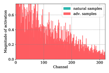
(a) $\mathcal{XE}$

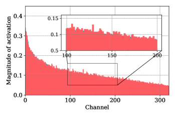
(b) TRADES

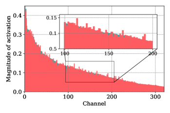
(c) ALP

(d) PGD-AT

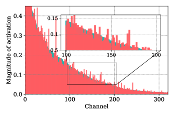
(e) SAT

(f)  OTJR (Ours)

Figure 8. Magnitude of activation at the penultimate layer for models trained with different defense methods. Our OTJR  can regulate adversarial samples’ magnitudes similar to clean samples’ while well suppressing both of them.

Appendix F Broader Impact

Utilizing machine learning models in real-world systems necessitates not only high accuracy but also robustness across diverse environmental scenarios. The central motivation of this study is to devise a training framework that augments the robustness of Deep Neural Network (DNN) models in the face of various adversarial attacks, encompassing both white-box and black-box methodologies. To realize this objective, we introduce the OTJR framework, an innovative approach that refines traditional Jacobian regularization techniques and aligns output distributions. This research represents a significant stride in synergizing adversarial training with input-output Jacobian regularization—a combination hitherto underexplored—to construct a more resilient model.

References

- (1)
- Andriushchenko et al. (2020) Maksym Andriushchenko, Francesco Croce, Nicolas Flammarion, and Matthias Hein. 2020. Square attack: a query-efficient black-box adversarial attack via random search. In European Conference on Computer Vision (ECCV). Springer, 484–501.
- Athalye et al. (2018) Anish Athalye, Nicholas Carlini, and David Wagner. 2018. Obfuscated gradients give a false sense of security: Circumventing defenses to adversarial examples. In International conference on machine learning. PMLR, 274–283.
- Bai et al. (2021) Yang Bai, Yuyuan Zeng, Yong Jiang, Shu-Tao Xia, Xingjun Ma, and Yisen Wang. 2021. Improving adversarial robustness via channel-wise activation suppressing. International Conference on Learning Representations (ICLR) (2021).
- Bortsova et al. (2021) Gerda Bortsova, Cristina Gonzalez-Gonzalo, Suzanne Wetstein, Florian Dubost, Ioannis Katramados, Laurens Hogeweg, Bart Liefers, Bram Ginneken, Josien Pluim, Mitko Veta, et al. 2021. Adversarial attack vulnerability of medical image analysis systems: Unexplored factors. Medical Image Analysis (2021), 102141.
- Bouniot et al. (2021) Quentin Bouniot, Romaric Audigier, and Angelique Loesch. 2021. Optimal transport as a defense against adversarial attacks. In 2020 25th International Conference on Pattern Recognition (ICPR). IEEE, 5044–5051.
- Bui et al. (2022) Tuan Anh Bui, Trung Le, Quan Tran, He Zhao, and Dinh Phung. 2022. A unified wasserstein distributional robustness framework for adversarial training. arXiv preprint arXiv:2202.13437 (2022).
- Carlini et al. (2019) Nicholas Carlini, Anish Athalye, Nicolas Papernot, Wieland Brendel, Jonas Rauber, Dimitris Tsipras, Ian Goodfellow, Aleksander Madry, and Alexey Kurakin. 2019. On evaluating adversarial robustness. arXiv preprint arXiv:1902.06705 (2019).
- Carlini and Wagner (2017) Nicholas Carlini and David Wagner. 2017. Towards evaluating the robustness of neural networks. In 2017 ieee symposium on security and privacy (sp). IEEE, 39–57.
- Christian et al. (2013) Szegedy Christian, Zaremba Wojciech, Sutskever Ilya, Bruna Joan, Erhan Dumitru, Goodfellow Ian, and Fergus Rob. 2013. Intriguing properties of neural networks. arXiv preprint arXiv:1312.6199 (2013).
- Co et al. (2021) Kenneth T Co, David Martinez Rego, and Emil C Lupu. 2021. Jacobian Regularization for Mitigating Universal Adversarial Perturbations. 30th International Conference on Artificial Neural Networks (ICANN) (2021).
- Croce and Hein (2020a) Francesco Croce and Matthias Hein. 2020a. Minimally distorted adversarial examples with a fast adaptive boundary attack. In International Conference on Machine Learning (ICML). PMLR, 2196–2205.
- Croce and Hein (2020b) Francesco Croce and Matthias Hein. 2020b. Reliable evaluation of adversarial robustness with an ensemble of diverse parameter-free attacks. In International conference on machine learning. PMLR, 2206–2216.
- Cui et al. (2021) Jiequan Cui, Shu Liu, Liwei Wang, and Jiaya Jia. 2021. Learnable boundary guided adversarial training. In Proceedings of the IEEE/CVF International Conference on Computer Vision. 15721–15730.
- Cuturi (2013) Marco Cuturi. 2013. Sinkhorn distances: Lightspeed computation of optimal transport. Advances in neural information processing systems (NeurIPS) 26 (2013), 2292–2300.
- Deng et al. (2020) Yao Deng, Xi Zheng, Tianyi Zhang, Chen Chen, Guannan Lou, and Miryung Kim. 2020. An analysis of adversarial attacks and defenses on autonomous driving models. In 2020 IEEE International Conference on Pervasive Computing and Communications (PerCom). IEEE, 1–10.
- Dong et al. (2018) Yinpeng Dong, Fangzhou Liao, Tianyu Pang, Hang Su, Jun Zhu, Xiaolin Hu, and Jianguo Li. 2018. Boosting adversarial attacks with momentum. In Proceedings of the IEEE conference on computer vision and pattern recognition (CVPR). 9185–9193.
- Duchi et al. (2021) John C Duchi, Peter W Glynn, and Hongseok Namkoong. 2021. Statistics of robust optimization: A generalized empirical likelihood approach. Mathematics of Operations Research 46, 3 (2021), 946–969.
- Gao et al. (2022) Rui Gao, Xi Chen, and Anton J Kleywegt. 2022. Wasserstein distributionally robust optimization and variation regularization. Operations Research (2022).
- Guo et al. (2019) Chuan Guo, Jacob Gardner, Yurong You, Andrew Gordon Wilson, and Kilian Weinberger. 2019. Simple black-box adversarial attacks. In International Conference on Machine Learning (ICML). PMLR, 2484–2493.
- Helgason (2010) Sigurdur Helgason. 2010. Integral geometry and Radon transforms. Springer Science & Business Media.
- Hoffman et al. (2019) Judy Hoffman, Daniel A Roberts, and Sho Yaida. 2019. Robust learning with Jacobian regularization. arXiv preprint arXiv:1908.02729 (2019).
- Ian et al. (2014) Goodfellow Ian, Shlens Jonathon, and Szegedy Christian. 2014. Explaining and harnessing adversarial examples. arXiv preprint arXiv:1412.6572 (2014).
- Jakubovitz and Giryes (2018) Daniel Jakubovitz and Raja Giryes. 2018. Improving DNN robustness to adversarial attacks using Jacobian regularization. In Proceedings of the European Conference on Computer Vision (ECCV). 514–529.
- Kannan et al. (2018) Harini Kannan, Alexey Kurakin, and Ian Goodfellow. 2018. Adversarial logit pairing. arXiv preprint arXiv:1803.06373 (2018).
- Krizhevsky et al. (2009) Alex Krizhevsky, Geoffrey Hinton, et al. 2009. Learning multiple layers of features from tiny images. Technical Report. University of Toronto, Toronto.
- Kuhn et al. (2019) Daniel Kuhn, Peyman Mohajerin Esfahani, Viet Anh Nguyen, and Soroosh Shafieezadeh-Abadeh. 2019. Wasserstein distributionally robust optimization: Theory and applications in machine learning. In Operations research & management science in the age of analytics. Informs, 130–166.
- Kurakin et al. (2016) Alexey Kurakin, Ian Goodfellow, Samy Bengio, et al. 2016. Adversarial examples in the physical world.
- Ma et al. (2021) Xingjun Ma, Yuhao Niu, Lin Gu, Yisen Wang, Yitian Zhao, James Bailey, and Feng Lu. 2021. Understanding adversarial attacks on deep learning based medical image analysis systems. Pattern Recognition 110 (2021), 107332.
- Madry et al. (2018) Aleksander Madry, Aleksandar Makelov, Ludwig Schmidt, Dimitris Tsipras, and Adrian Vladu. 2018. Towards deep learning models resistant to adversarial attacks. International Conference on Learning Representations (ICLR) (2018).
- Meng et al. (2019) Cheng Meng, Yuan Ke, Jingyi Zhang, Mengrui Zhang, Wenxuan Zhong, and Ping Ma. 2019. Large-scale optimal transport map estimation using projection pursuit. Advances in Neural Information Processing Systems (NeurIPS) (2019).
- Mladenovic et al. (2021) Andjela Mladenovic, Joey Bose, William L Hamilton, Simon Lacoste-Julien, Pascal Vincent, Gauthier Gidel, et al. 2021. Online Adversarial Attacks. In International Conference on Learning Representations.
- Moosavi-Dezfooli et al. (2016) Seyed-Mohsen Moosavi-Dezfooli, Alhussein Fawzi, and Pascal Frossard. 2016. Deepfool: a simple and accurate method to fool deep neural networks. In Proceedings of the IEEE conference on computer vision and pattern recognition. 2574–2582.
- Pang et al. (2020) Tianyu Pang, Xiao Yang, Yinpeng Dong, Hang Su, and Jun Zhu. 2020. Bag of tricks for adversarial training. arXiv preprint arXiv:2010.00467 (2020).
- Petrovich et al. (2020) Mathis Petrovich, Chao Liang, Ryoma Sato, Yanbin Liu, Yao-Hung Hubert Tsai, Linchao Zhu, Yi Yang, Ruslan Salakhutdinov, and Makoto Yamada. 2020. Feature robust optimal transport for high-dimensional data. arXiv preprint arXiv:2005.12123 (2020).
- Qian (1999) Ning Qian. 1999. On the momentum term in gradient descent learning algorithms. Neural networks 12, 1 (1999), 145–151.
- Rahimian and Mehrotra (2019) Hamed Rahimian and Sanjay Mehrotra. 2019. Distributionally robust optimization: A review. arXiv preprint arXiv:1908.05659 (2019).
- Rice et al. (2020) Leslie Rice, Eric Wong, and Zico Kolter. 2020. Overfitting in adversarially robust deep learning. In International Conference on Machine Learning. PMLR, 8093–8104.
- Rony et al. (2019) Jérôme Rony, Luiz G Hafemann, Luiz S Oliveira, Ismail Ben Ayed, Robert Sabourin, and Eric Granger. 2019. Decoupling direction and norm for efficient gradient-based l2 adversarial attacks and defenses. In Proceedings of the IEEE/CVF Conference on Computer Vision and Pattern Recognition (CVPR). 4322–4330.
- Shafahi et al. (2019) Ali Shafahi, Mahyar Najibi, Amin Ghiasi, Zheng Xu, John Dickerson, Christoph Studer, Larry S Davis, Gavin Taylor, and Tom Goldstein. 2019. Adversarial training for free! arXiv preprint arXiv:1904.12843 (2019).
- Shafieezadeh Abadeh et al. (2015) Soroosh Shafieezadeh Abadeh, Peyman M Mohajerin Esfahani, and Daniel Kuhn. 2015. Distributionally robust logistic regression. Advances in Neural Information Processing Systems 28 (2015).
- Vialard (2019) François-Xavier Vialard. 2019. An elementary introduction to entropic regularization and proximal methods for numerical optimal transport. (2019).
- Villani (2008) Cédric Villani. 2008. Optimal transport: old and new. Vol. 338. Springer Science & Business Media.
- Wu et al. (2020) Dongxian Wu, Shu-Tao Xia, and Yisen Wang. 2020. Adversarial weight perturbation helps robust generalization. Advances in Neural Information Processing Systems 33 (2020), 2958–2969.
- Zagoruyko and Komodakis (2016) Sergey Zagoruyko and Nikos Komodakis. 2016. Wide residual networks. arXiv preprint arXiv:1605.07146 (2016).
- Zhang and Wang (2019) Haichao Zhang and Jianyu Wang. 2019. Defense against adversarial attacks using feature scattering-based adversarial training. Advances in Neural Information Processing Systems (NeurIPS) 32 (2019), 1831–1841.
- Zhang et al. (2019) Hongyang Zhang, Yaodong Yu, Jiantao Jiao, Eric Xing, Laurent El Ghaoui, and Michael Jordan. 2019. Theoretically principled trade-off between robustness and accuracy. In International Conference on Machine Learning (ICML). PMLR, 7472–7482.
- Zhang et al. (2020) Jingfeng Zhang, Jianing Zhu, Gang Niu, Bo Han, Masashi Sugiyama, and Mohan Kankanhalli. 2020. Geometry-aware instance-reweighted adversarial training. International Conference on Learning Representations (ICLR) (2020).