Probabilistic Domain Adaptation for Biomedical Image Segmentation

Abstract

Segmentation is a key analysis tasks in biomedical imaging. Given the many different experimental settings in this field, the lack of generalization limits the use of deep learning in practice. Domain adaptation is a promising remedy: it trains a model for a given task on a source dataset with labels and adapts it to a target dataset without additional labels. We introduce a probabilistic domain adaptation method, building on self-training approaches and the Probabilistic UNet. We use the latter to sample multiple segmentation hypothesis to implement better pseudo-label filtering. We further study joint and separate source-target training strategies and evaluate our method on three challenging domain adaptation tasks for biomedical segmentation.

1 Introduction

Deep learning has emerged as the standard approach for many image analysis tasks, including segmentation in biomedical imaging. However, its practical application is often hindered by the limited generalization and the need for large labeled training datasets in supervised learning. These drawbacks are particularly challenging in biomedical imaging, where many different experimental setups and modalities exist. Domain adaptation has emerged as a promising remedy: It adapts a model that was trained on a labeled dataset (”source”) for a specific task, for example cell segmentation, to solve the same task on a new dataset (”target”) from a different domain. We present a novel domain adaptation method that combines self-training techniques with probabilistic segmentation and demonstrate its effectiveness for semantic segmentation in biomedical images. Our proposed method shows significant promise in improving generalization across domains and reducing the labeling effort in practice.

Self-training for domain adaptation builds on ideas from semi-supervised learning. These approaches train a model jointly on the labeled and unlabeled data. On the unlabeled data, predictions from a version of the model (the teacher) are used as so-called pseudo-labels for the model (the student). A popular self-training method is Mean Teacher [20], which uses the exponential moving average (EMA) of the student weights to compute the teacher weights. Recently FixMatch [17] has gained popularity. Its teacher and student share weights, but weak and strong augmentations prevent collapse of the model predictions. Both approaches have been studied for semi-supervised classification as well as segmentation, for example in UniMatch [23]. Self-training can be extended to domain adaptation, see for example AdaMatch [2].

We study three key design choices for applying self-training to domain adaptation: (i) how to generate the pseudo-labels, (ii) how to filter them and (iii) how to orchestrate source and target training. Mean Teacher, FixMatch and others have mostly focused on (i), by studying different student-teacher set-ups and different augmentation strategies. For (ii) most approaches either do not filter the pseudo-labels (e.g. MeanTeacher), or filter them based on confidences derived from deterministic model predictions (e.g. FixMatch). However, regular deep learning methods are known to be badly calibrated and hence their predictions do not yield reliable confidence estimates. Instead, we propose to use the Probabilistic UNet (PUNet) [8], a probabilistic segmentation method, to derive better confidence estimates, and use them to filter pseudo-labels. Fig. 1 shows an overview of our method. We also investigate two different strategies for (iii): separate source training and subsequent adaptation (two stages) versus joint training on source and target (single stage). We evaluate our method on three challenging domain adaptation tasks in biomedical segmentation: cell segmentation in livecell microscopy, mitochondria segmentation in electron microscopy (EM) and lung segmentation in X-Ray. Our method compares favorably to strong baselines. Code is available at https://github.com/computational-cell-analytics/Probabilistic-Domain-Adaptation.

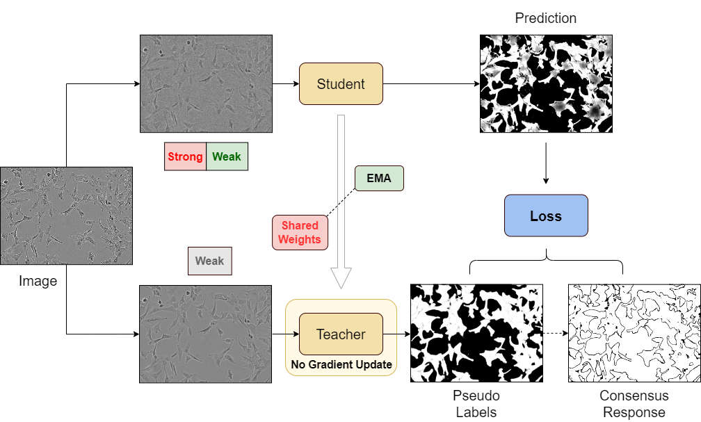
Figure 1: Self-training and probabilistic segmentation: the teacher predicts pseudo-labels, which are used to compute the loss with the student predictions. Multiple samples from the (prob.) teacher are used to filter the pseudo-labels. Student and teacher either share weights (FixMatch, red) or the teacher weights are the EMA of the student weights (MeanTeacher, green). Their inputs are transformed with different weak (MeanTeacher) or weak and strong (FixMatch) augmentations.

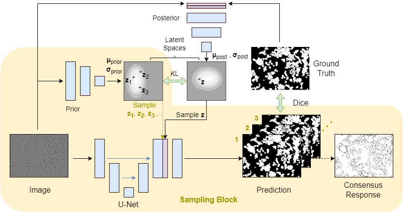
Figure 2: PUNet set-up: during training both prior and posterior encoder predict parameters for sampling latents. Features from the UNet are concatenated with the posterior latents for prediction. The KL divergence minimizes the distance between prior and posterior predictions, the dice loss between segmentation and labels. In inference the prior encoder is used for sampling.

2 Related Work

Self-training:

These methods are among the most popular approaches in semi-supervised learning; examples include Mean Teacher [20], ReMixMatch [1] and FixMatch [17]. They are often studied for classification tasks, but have also been successfully applied to semantic segmentation, see for example PseudoSeg [27] and UniMatch [23]. Similar methods have emerged for domain adaptation:a unified framework for semi-supervision and domain adaptation has recently been proposed by AdaMatch [2]. Self-training methods for domain adaptation in segmentation have for example been introduced by Zou et al. [26], who use class-balanced pseudo-labeling, and Mei et al. [12], who use instance adaptive pseudo-labeling. Applications to segmentation in biomedical images include Shallow2Deep [11], which uses intermediate predictions from a shallow learner for pseudo-labels, and SPOCO [22], which uses a per-instance loss and self-training to learn from sparse instance segmentation labels.

Probabilistic segmentation:

Probabilistic segmentation methods learn a distribution over segmentation results and enable sampling from it. Early approaches have implemented this through test-time dropout [6], recent approaches such as the PUNet [8] and its hierarchical extension [9], use a conditional variational autoencoder. Prior work has introduced strategies for filtering pseudo-labels using probabilistic segmentation for semi-supervised learning; either using the dropout approach [24, 14] or inconsistencies between different models [15].

3 Methods

We propose a new approach to domain adaptation for semantic segmentation. We first introduce the self-training methodology (first paragraph), review its application to domain adaptation (second paragraph), review probabilistic segmentation (third paragraph), and explain how we combine these elements for probabilistic domain adaptation (fourth paragraph). Exact definitions for all terms are given in App. 0.A.

Self-training for semi-supervised learning:

Self-training approaches train a model using the labeled samples to compute a supervised loss term $L_{s}$ and the unlabeled samples to compute an unsupervised loss term $L_{u}$. The term $L_{u}$ is formulated based on a student-teacher set-up, which uses the teacher predictions as pseudo-labels. For the student the same model that is trained via $L_{s}$ is used, the teacher is derived from it (e.g. by weight sharing or EMA of the weights). To avoid over-fitting to the teacher predictions, the inputs to the student and teacher are transformed with different augmentations and the pseudo-labels are filtered and/or post-processed. Denoting the supervised inputs and labels as $x_{s}$ and $y_{s}$, the inputs without labels as $x_{u}$, the student and teacher model as $s$ and $t$, the augmentations for the student and teacher as $\tau_{s}$ and $\tau_{t}$, the function that filters the pseudo-labels as $f$ and the function that post-processes them as $p$, we can write the generation of pseudo-labels $\hat{y}_{u}$ and the combined loss $L$ as:

$$\hat{y}_{u}=p(t(\tau_{t}(x_{u}))),$$ (1)

$$L=L_{s}(s(x_{s}),\,y_{s})+L_{u}(f(s(\tau_{s}(x_{u})),\,\hat{y}_{u})).$$ (2)

The operations in Eq. 1 are not taken into account for the gradient computation. We obtain MeanTeacher [20] from Eq. 1 and 2 by choosing $\tau_{s}$ and $\tau_{t}$ to be weak augmentations from the same distribution, choosing both $f$ and $p$ to be the identity function (i.e. pseudo-labels are neither filtered nor post-processed), and computing the teacher weights $w_{t}$ as the EMA of the student weights $w_{s}$: $w_{t}=\alpha\,w_{t}+(1-\alpha)\,w_{s}$ with $\alpha$ close to 1. We obtain FixMatch [17] by choosing $\tau_{s}$ to be strong augmentations, $\tau_{t}$ to be weak augmentations, $t$ to share weights with $s$, $f$ to filter out predictions with a probability below a given threshold, and $p$ to set the predicted values to 1 if they are above that threshold. We apply MeanTeacher and FixMatch to semantic segmentation. Our modifications for this task, including the choices for $L_{s}$ and $L_{u}$, are given in the last paragraph.

Self-training for domain adaptation:

There are two possible strategies for applying the self-training procedures from the previous paragraph to domain adaptation: in the joint strategy the model is trained according to Eq. 1 and 2 using the source data as labeled samples $(x_{s},y_{s})$ and the target data as unlabeled samples $x_{u}$. In the separate strategy the model is pre-trained on the source domain, using the supervised loss $L_{s}$, and then adapted to the target domain, using the unsupervised loss $L_{u}$. The joint strategy is a direct extension of semi-supervised learning to domain adaptation, as AdaMatch [2] has shown through a unified formulation of both learning paradigms. In contrast, the separate strategy requires two training stages, which complicates the set-up. However, it has the practical advantage that only a single model has to be pre-trained per task, which can then be fine-tuned for a new target dataset without access to the source data and with a small computational budget. In comparison, the joint strategy requires training a model for each source-target pair, with access to the source data. Here, we compare both domain adaptation strategies.

Probabilistic segmentation:

Probabilistic segmentation methods have been introduced to account for the inherent uncertainty of the segmentation tasks: in many cases there is not a single ”true” segmentation solution, but rather a distribution. For example, in the case of radiology, lesions are often annotated differently by experts, without a definite consensus solution. To model this label uncertainty, probabilistic segmentation methods enable sampling diverse segmentation results instead of providing a deterministic result. Here, we use the PUNet [8]: it combines a UNet [13], which learns deterministic features, with a conditional variational autoencoder [18] that enables sampling. During training it uses a prior encoder, which sees only the images, and a posterior encoder, which sees the images and labels. Both encoders map their respective inputs to the parameters of a multi-dimensional gaussian distribution; sampling from it yields representations in a latent space. The latent samples from the posterior and the UNet features are concatenated and passed to additional layers to obtain the segmentation result. The architecture is trained using a variational loss term $L_{var}$ that minimizes the distance between the distributions of the prior and posterior encoder, and a reconstruction loss term $L_{rec}$ that minimizes the difference between prediction and labels. For inference the prior encoder is used for sampling. See Fig. 2 for an overview of the PUNet architecture and training.

Here, we use the PUNet to sample diverse predictions and implement better pseudo-label filtering compared to thresholding the predictions of a deterministic model. We introduce the consensus response $C$. Given predictions $m(x_{i})^{k}_{j}$ from a PUNet $m$ for pixel $i$, class $k$ and sample $j$, the per pixel response $c_{i}$ is:

$$c_{i}=\frac{1}{N}\sum_{j}^{N}\,\{1\,\textrm{if}\,t(x_{i})^{k}_{j}\geq\theta\,\textrm{for any}\,k\in K\ \,\textrm{else}\,0\}.$$ (3)

Here, $\theta$ denotes the threshold parameter, $N$ the number of samples and $K$ the number of classes. This expression generalizes the thresholding approach for a single prediction, which is recovered for $N=1$. See the next paragraph for how $C$ is used for pseudo-label filtering.

Probabilistic domain adaptation:

We combine the elements from the previous paragraphs into a family of methods for probabilistic domain adaptation. We follow the PUNet implementation of [8], but use the dice score for $L_{rec}$ instead of the cross entropy. We use the same loss function ($L=L_{var}+L_{rec}$) for both $L_{s}$ and $L_{u}$ (see Eq. 2). We do not use pseudo-label post-processing, i.e. $p$ is the identity (cf. Eq 1). We study two different settings for self-training: for MeanTeacher $\tau_{s}$ and $\tau_{t}$ are both weak augmentations and the teacher weights are the EMA of the student weights. For FixMatch $\tau_{s}$ are strong augmentations, $\tau_{t}$ are weak augmentations and the student and teacher share weights. We use the consensus response $C$ (Eq. 3) for filtering the reconstruction loss $L_{rec}$. Here, we explore three different settings: consensus masking, which masks the pixels that do not fulfill $c_{i}=1$, consensus weighting, which weights the loss with the value of $c_{i}$, and no filtering. The set-up for unsupervised training is shown in Fig.1. We also investigate both the joint and separate domain adaptation strategies. Tab. 1 gives an overview of the proposed methods and the corresponding abbreviations. Pseudo-code for the methods can be found in App 0.B.

Table 1: Proposed probabilistic domain adaptation methods and abbreviations.

	FixMatch			MeanTeacher
	cons. masking	cons. weighting	none	cons. masking	cons. weighting	none
joint	$FM^{m}_{j}$	$FM^{w}_{j}$	$FM_{j}$	$MT^{m}_{j}$	$MT^{w}_{j}$	$MT_{j}$
separate	$FM^{m}_{s}$	$FM^{w}_{s}$	$FM_{j}$	$MT^{m}_{s}$	$MT^{w}_{s}$	$MT_{s}$

4 Results

We perform experiments for three different domain adaptation settings: cell segmentation in livecell microscopy, mitochondria segmentation in EM and lung segmentation in X-Ray. Model implementation and hyperparameters are documented in detail in App. 0.C, the datasets in App. 0.D.

4.1 Domain Adaptation Results

We perform comprehensive experiments for cell segmentation in livecell microscopy. We use data from LiveCELL [3], which contains 5,000 images with cell instance labels for 8 different cell lines. We transform the instance labels to binary masks for semantic segmentation, treat each cell line as a different domain and evaluate the segmentation quality for all source target pairs. In Tab.  2 the averaged dice scores for each source domain applied to the 7 corresponding target domains are given. We evaluate four of our approaches ($MT_{s}^{m},MT_{s},FM_{j}^{m},FM_{j}$), a separate and a joint adaptation strategy, with and without masking. For the $MT$ approaches we use blurring and additive noise as augmentations, and for $FM$ stronger blurring, noise as and contrast shifts as strong augmentations. We compare to the following baselines: UNet ($UNet$), PUNet ($PUNet$) and the method from [3] (LiveCELL) are trained on source and applied directly to the target, $PUNet_{trg}$ is a simpler adaptation strategy that uses pseudo-labels predicted by the source PUNet for training from scratch, $PUNet_{trg}^{m}$ additionally uses masking. More results can be found in App. 0.E.

Table 2: Livecell segmentation results. Methods above the midline do not use adaptation, italic means trained by us and same network architecture.

Method	A172	BT474	BV2	Huh7	MCF7	SHSY5Y	SkBr3	SKOV3
$UNet$	0.87	0.82	0.68	0.71	0.85	0.81	0.82	0.86
$PUNet$	0.87	0.83	0.49	0.79	0.86	0.79	0.72	0.88
LiveCELL	0.84	0.81	0.30	0.79	0.75	0.79	0.81	0.87
$PUNet_{trg}$	0.88	0.84	0.51	0.81	0.86	0.79	0.73	0.88
$PUNet_{trg}^{m}$	0.89	0.86	0.54	0.82	0.87	0.84	0.73	0.89
$MT_{s}$	0.87	0.83	0.54	0.79	0.87	0.81	0.70	0.87
$MT_{s}^{m}$	0.88	0.86	0.76	0.83	0.89	0.88	0.69	0.88
$FM_{j}$	0.88	0.88	0.81	0.88	0.88	0.86	0.87	0.86
$FM_{j}^{m}$	0.86	0.88	0.82	0.88	0.88	0.81	0.85	0.87

We see that some adaptation tasks (A172, BT474, SHSY5Y, SKOV3) are easy and all methods perform similar. For the more difficult tasks (BV2, Huh7, SkBr3) the self-training approaches, in particular $FM_{j}$ and $FM_{j}^{m}$, significantly improve the results. We see a clear advantage of masking for $MT$, but no significant effect on $PUNet_{trg}$ and $FM_{j}$. Qualitative results are shown in Fig. 3.

We demonstrate the potential of our approach for EM mitochondria segmentation, using MitoEM [21] as source dataset. It contains two large volumes with instance labels that we binarize for semantic segmentation. We use the datasets from Lucchi [10] and VNC [4] as targets and address 2d segmentation. Tab.  4 shows the results. We only use the $MT_{s}$ approaches since joint training would take long due to the large source data. We include $UNet$ and $PUNet$ trained on MitoEM. Our methods significantly improve results, in particular $MT_{s}^{w}$.

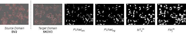
Figure 3: Qualtiative results for livecell segmentation: left image shows the source domain with labels, right shows the target domain, including predictions from four methods, PUNet trained on source, adapted to target, and two self-training approaches.

Table 3: EM Segmentation.

Method	Lucchi	VNC
$UNet$	0.86	0.59
$PUNet$	0.80	0.46
$MT_{s}$	0.81	0.63
$MT_{s}^{m}$	0.84	0.73
$MT_{s}^{w}$	0.90	0.74

Table 4: X-Ray segmentation.

Method	NIH	Montgomery	JSRT1	JSRT2
$UNet$	0.77	0.78	0.72	0.08
$PUNet$	0.76	0.75	0.73	0.12
$MT_{s}$	0.78	0.77	0.77	0.12
$MT_{s}^{m}$	0.78	0.77	0.77	0.11
$MT_{j}$	0.78	0.77	0.69	0.21
$MT_{j}^{m}$	0.82	0.80	0.73	0.21

We also demonstrate the potential for medical imaging, using three datasets for X-Ray lung segmentation: NIH [19], Montgomery [5] and JSRT [16]. The latter contains two set-ups, so we obtain 4 domains and study the adaptation between all pairs. We only study $MT$ methods, and compare to the source $UNet$ and $PUNet$ baselines. Our methods improve results for most settings, masking is beneficial for $MT_{j}$ and does not have a significant effect for $MT_{s}$. Note that JSRT2 consists of inverted XRay image and presents a hard adaptation task. While none of the methods succeed, $MT_{j}$ shows better relative performance.

4.2 Ablation Studies

We study pseudo-label filtering (masking $m$, weighting $w$, no filtering) in more detail. Tab. 6 shows the results for the difficult livecell adaptation settings. We see that filtering consistently improves results, except for $FM_{j}$ where it does not have a significant effect. In most cases masking yields better results than weighting, except for $MT_{j}$. In Tab. 6 we investigate the two adaptation strategies. We see that joint training, in particular $FM_{j}$ yields overall better results, $FM_{s}$ yields inferior results and we have observed unstable training for this method.

Table 5: Pseudo-label filtering.

Method	BV2	Huh7	SkBr3
$MT_{s}$	0.54	0.79	0.70
$MT_{s}^{m}$	0.76	0.83	0.69
$MT_{s}^{w}$	0.65	0.79	0.74
$MT_{j}$	0.64	0.68	0.59
$MT_{j}^{m}$	0.83	0.75	0.63
$MT_{j}^{w}$	0.78	0.85	0.81
$FM_{j}$	0.81	0.88	0.87
$FM_{j}^{m}$	0.82	0.88	0.85
$FM_{j}^{w}$	0.69	0.77	0.86

Table 6: Domain adaptation strategies.

Method	BV2	Huh7	SkBr3
$MT_{s}$	0.54	0.79	0.70
$MT_{s}^{m}$	0.76	0.83	0.69
$MT_{j}$	0.64	0.68	0.59
$MT_{j}^{m}$	0.83	0.75	0.63
$FM_{s}$	0.43	0.74	0.74
$FM_{s}^{m}$	0.52	0.79	0.70
$FM_{j}$	0.81	0.88	0.87
$FM_{j}^{m}$	0.82	0.88	0.85

5 Discussion

Among our probabilistic domain adaptation methods $FM_{j}$ shows the best overall performance, while $MT_{s}$ is competitive in may settings. It can be shipped as pre-trained model, a clear practical advantage. Pseudo-label filtering via consensus masking improves quality in most cases, in particular for difficult adaptation tasks. It does not always yield better results; we hypothesize that this is due to low masking rates and plan to investigate mitigation strategies. We see the potential to improve our methods via better probabilistic segmentation (e.g. [7]) and better strong augmentations, e.g. CutMix [25], which has shown success in semi-supervision [23]. We envision that these improvements will yield competitive $MT_{s}$ or $FM_{s}$ strategies to build user friendly tools. Finally, we plan to extend our approach to instance segmentation see App. 0.F.

6 Acknowledgments

We would like to express their gratitude to Sartorius AG for support of this re- search through the Quantitative Cell Analytics Initiative (QuCellAI) and would also like to extend our thanks to all partners involved in the initiative for their contributions and valuable insights. We also gratefully acknowledge the com- puting time granted by the Resource Allocation Board and provided on the supercomputer Lise and Emmy at NHR@ZIB and NHR@Göttingen as part of the NHR infrastructure. The calculations for this research were conducted with computing resources under the project nim00007.

Appendix 0.A Definition of Terms

We address the problem of unsupervised domain adaptation (UDA). This problem is closely related to supervised domain adaptation (SDA) and semi-supervised learning (SSL). In SSL problems both labeled and unlabeled training data is given, with the goal to learn a ”better” model using all available data compared to using fully supervised learning on just the labeled data. Both labeled and unlabeled data are from the same domain (same data distribution). In the case of UDA a source domain with labels and a target domain without labels is given. Source and target domain have different data distributions, corresponding e.g. to different imaging devices or different experimental conditions in biomedical applications. The goal of UDA is to train a model that solves the same task (e.g. cell segmentation) on the target domain as on the source domain. The case of SDA is very similar, but the target domain is partially labeled (i.e. annotations are provided for a subset of the target samples). This discussion shows that all three settings are similar, with the distinction being the data distributions for labeled and unlabeled data: In SSL both labeled and unlabeled data come from the same data distribution and in UDA they come from two different data distributions (source and target data distribution). In SDA the labeled data comes from both source and target distribution (usually with the fraction of target data being significantly smaller) and the unlabeled data comes only from the target distribution. Consequently self-training methods can be generalized to all three learning problems, as has recently been demonstrated by AdaMatch [2]. Using the same recipe, our method is applicable to SSL and SDA as well; in fact we apply it in a SSL fashion in our proof-of-concept for instance segmentation (see App. 0.F).

We make use of self-training with pseudo-labels to address UDA. These terms are sometimes used with slightly different meanings in the literature. Here, we use self-training to describe methods that use a version of the model being trained to generate predictions on unlabeled data, which are then used as targets in an unsupervised loss function to again train the model. This can be understood as a student-teacher set-up, with the teacher being a version of the student (e.g. through EMA of weights or weight sharing). We use the term pseudo-labeling to describe the process of transforming the teacher predictions into targets for the unsupervised loss function, e.g. by post-processing or filtering (masking or weighting) them. Note that the literature sometimes distinguish between pseudo-labeling when the likeliest prediction is used as hard target in the unsupervised loss, and consistency regularization when the softmax output (more generally output after the last activation) is used as target. See for example https://lilianweng.github.io/posts/2021-12-05-semi-supervised/ for an in-depth discussion. However, this distinction is minor in practice and can be incorporated in the pseudo-labeling post-processing in our formulation (the function $p$ in Eq. 1). Hence, we do not make this distinction throughout the paper.

Appendix 0.B Probabilistic Domain Adaptation: Training Strategies

We implement two different approaches to domain adaptation: joint training (model is trained jointly on labeled source and unlabeled target data, using a supervised and unsupervised loss function) and separate training (model is first pre-trained on the labeled source data, using only the supervised loss, and then fine-tuned on the unlabeled target data, using only the unsupervised loss). Here, we show pseudo-code for the two training routines, for joint training in Alg. 1 and for separate training in Alg. 2. For simplicity we omit validation, which is performed using the target data in both cases. Here, we use the same loss function $l$ for both the supervised and unsupervised loss.

Input: Labeled training data {($x_{s}$, $y_{s}$)}, unlabeled training data {$x_{u}$}, teacher and student models $s$, $t$, number of iterations $N$

Initialize parameters of $s$ and $t$;

for $i\leftarrow 1$ to $N$ do

       Sample mini-batch ($x_{s}^{i}$, $y_{s}^{i}$) and $x_{u}^{i}$;

       Compute supervised loss $L_{s}=l(s(x_{s}^{i}),y_{s}^{i})$;

       Sample augmentations $\tau_{s}$ and $\tau_{t}$;

       Compute pseudo-labels $\hat{y}=t(\tau_{t}(x_{u}))$;

       Compute unsupervised loss $L_{u}=l(f(s(\tau_{s}(x_{s})),\hat{y}))$;

       Compute gradients, update parameters of $s$ based on $L_{s}+L_{u}$;

       Update parameters of $t$ from $s$;

end for

Algorithm 1 Pseudo code for the joint training strategy.

Input: Unlabeled training data {$x_{u}$}, pre-trained model $s$, number of iterations $N$

Copy model $t$ from $s$;

for $i\leftarrow 1$ to $N$ do

       Sample mini-batch $x_{u}^{i}$;

       Sample augmentations $\tau_{s}$ and $\tau_{t}$;

       Compute pseudo-labels $\hat{y}=t(\tau_{t}(x_{u}))$;

       Compute unsupervised loss $L_{u}=l(f(s(\tau_{s}(x_{s})),\hat{y}))$;

       Compute gradients, update parameters of $s$ based on $L_{u}$;

       Update parameters of $t$ from $s$;

end for

Algorithm 2 Pseudo code for the separate training strategy. (Only the adaptation stage on the target domain; source training follows regular supervised learning.)

The two self-training approaches we implement, MeanTeacher and AdaMatch correspond to different choices for the teacher and student augmentations $\tau_{s}$ and $\tau_{t}$ as well as the teacher update scheme. For MeanTeacher both $\tau_{s}$ and $\tau_{t}$ are sampled from a distribution of weak augmentations and the weights of $t$ are the EMA of $s$. For FixMatch $\tau_{s}$ is sampled from a distribution of strong augmentations and $\tau_{t}$ from a distribution of strong augmentations, $s$ and $t$ share weights. The different pseudo-label filtering approaches are realized by different choices for $f$, where consensus masking corresponds to only computing gradients for pixels that have a value of 1 in the consensus response (see Eq. 3), consensus weighting corresponds to weighting the loss by the consensus response. In the case of no filtering $f$ is the identity.

Appendix 0.C Implementation

We use the same UNet and PUNet architecture for all experiments, using an encoder-decoder architecture following the respective implementations of [13] and [8]. We increase the number of channels from 64 to 128, 256 and 512 in the encoder, and decrease it accordingly in the decoder. We use 2D segmentation network, hence both architectures make use of 2d convolutions, 2d max-pooling and 2d upsampling operations. The UNet is trained using the Dice Error (1. - Dice Score) as loss function. For the PUNet we use a similar formulation for the loss function as in [8], but use the Dice Error for the reconstruction term in stead of the cross entropy. We use a dimension of 6 for the latent space predicted by the prior and posterior net of the PUNet. We use the Adam optimizer, relying on the default PyTorch parameter settings, except for the learning rate, and we use the ReduceLROnPlateau learning rate scheduler. For joint and source model trainings we train for 100k iteration, for the second stage of separate trainings we train for 10k iterations. We use different patch shapes, batch sizes and learning rates depending on the dataset and method; these values were determined by exploratory experiments. For LiveCELL:

• $UNet$: patch shape: (256, 256); batch size: 4; learning rate: 1e-4

• $PUNet$: patch shape: (512, 512); batch size: 4; learning rate: 1e-5

• $PUNet_{trg}$, $MT_{s}$: patch shape: (512, 512); batch size: 2; learning rate: 1e-5

• $FM_{s}$: patch shape: (256, 256); batch size: 2; learning rate: 1e-7

• $FM_{j}$, $MT_{j}$: patch shape: (256, 256); batch size: 2; learning rate: 1e-5

For mitochondria segmentation in EM:

• $UNet$, $PUNet$: patch shape: (512, 512); batch size: 2; learning rate: 1e-5

• $MT_{s}$: (256, 256); batch size: 2; learning rate: 1e-5

For lung segmentation in X-Ray:

• $UNet$: patch shape: (256, 256); batch size: 2; learning rate: 1e-4

• $PUNet$, $MT_{s}$, $MT_{j}$: patch shape: (256, 256); batch size: 2; learning rate: 1e-5

We use gaussian blurring and additive gaussian noise (applied randomly with a probability of 0.25, and with augmentations parameters also sampled from a distribution) as weak augmentations, and gaussian blurring, additive gaussian noise and random contrast adjustments (applied randomly with a probability of 0.5, and sampling from a wider range compared to the weak augmentations) as strong augmentations.

Our implementation is based on PyTorch. We use the PUNet implementation from https://github.com/stefanknegt/Probabilistic-Unet-Pytorch. All our code is available on github at https://github.com/computational-cell-analytics/Probabilistic-Domain-Adaptation. Please refer to the README for instructions on how to run and install it.

Appendix 0.D Datasets

LiveCELL Dataset

We use the LiveCELL dataset from [3]. This dataset contains about 5000 phase contrast microscopy images with instance segmentation ground-truth and predefined train-, test-, and validation-splits. We binarize the instance segmentation ground-truth to obtain a semantic segmentation problem. The dataset contains images of 8 different cell lines: A172, BT474, BV2, Huh7, MCF7, SHSY5Y, SkBr3 and SKOV3. These cell lines show significant difference in appearance and morphology of cells as well as spatial distribution such as cell density and cell clustering. Hence, we treat all 8 cell types as different domains, and study the adaptation from one cell line as source domain to the seven other target domains for all 8 cell lines. The columns in Tab. 2 show the average dice score for one source applied to the seven target domains.

Mitochondria EM Segmentation

For mitochondria segmentation in EM we use the dataset of [21] as source dataset. This dataset contains two EM volumes, one of human neural tissue, the other of rat neural tissue, imaged with scanning EM. Each volume contains 400 images with instance annotations for training, and 100 images with instance annotations for testing. We binarize the instance segmentation ground-truth to obtain a semantic segmentation problem. We study domain adaptation with [21] as source for two different target datasets. The first is Lucchi [10], which contains two volumes of tissue from the murine hippocampus imaged with FIBSEM that both contain mitochondria instance annotations. We use one of the volumes for training the domain adaptation methods (either via joint or separate training), and the other for evaluation. And VNC [4], which contains two volumes from the ventral nerve cord of a fruit fly, imaged with serial section transmission EM. Only one of the two volumes contains instance annotation, it is used for evaluation, the other does not, it is used for training the domain adaptation methods (which does not require labels).

Lung X-Ray Segmentation

For the lung segmentation task we use four different datasets of chest radiographs, following the experiment set-up of [19]. The datasets are: NIH, which contains chest X-Ray (CXR) images with various severity of lung diseases, Montgomery [5], which contains images of patients with and without tuberculosis, and JSRT [16], which contains images of patients with and without lung nodules. The JSRT dataset is split into two subsets: JSRT1 with normal CXR images (60 images, 50 train, 10 test), and JSRT2 with inverted CXR images (247 images, 199 train, 48 test). The NIH dataset contains 100 images (we use 80 for training and 20 for testing) and the Montgomery dataset contains 138 images (113 are used trainining, 25 for testing) respectively. All datasets contain binary lung annotations; we discard additional annotations in the case of JSRT2. We treat each dataset as a separate domain, and perform domain adaptation for all pairs of domains.

Appendix 0.E Livecell Segmentation Results

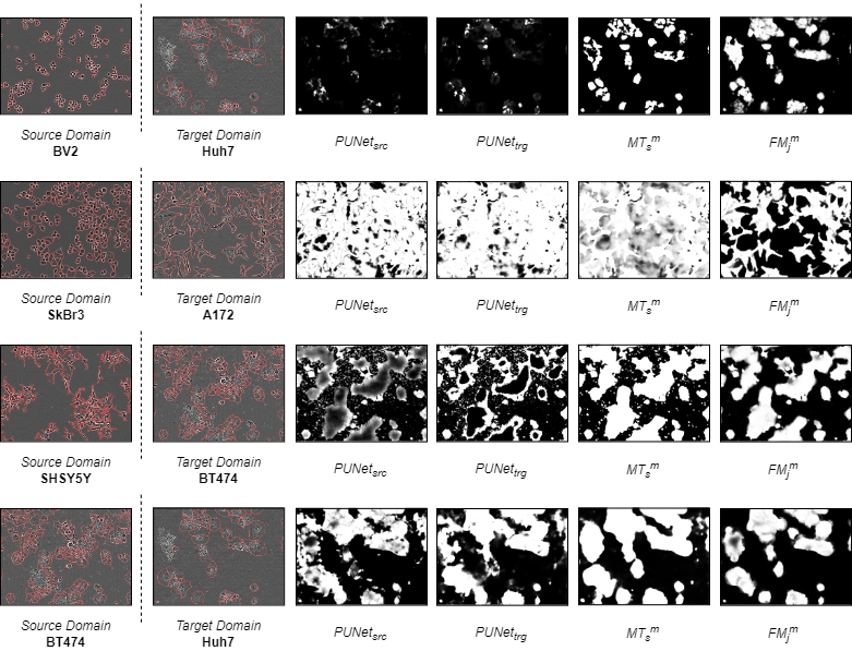
Figure 4: Qualtiative results for livecell segmentation: left image shows the source domain with labels, right shows the target domain, including predictions from four methods, PUNet trained on source, adapted to target, and two self-training approaches.

Appendix 0.F Extension to instance segmentation

We implement a proof-of-concept extension fo our approach to instance segmentation, using data from the NeurIPS Cell Segmentation Challenge (https://neurips22-cellseg.grand-challenge.org/). This dataset contains 1,000 training images with instance segmentation annotations, and 1,500 additional images without annotations. The images come from 4 different microscopy domains (Brightfield, Fluorescence, Phase-contrast, Differential inference contrast).

We adapt our approach to instance segmentation by predicting 2 channels: the cell foreground (same as in the LiveCELL experiments) and the cell boundaries. To obtain an instance segmentation we use a seeded watershed algorithm, using the boundary predictions as height map and connected components of the foreground predictions subtracted by boundary probabilities as seeds. We train a PUNet fully supervised on the data with labels, and compare it to predictions from all $MT_{j}$ variations ($MT_{j}$, $MT_{j}^{w}$, $MT_{j}^{m}$). Note that we train in a semi-supervised fashion here, and train the model jointly on all labeled and unlabeled data, without taking the different domains into account.

We have only studied the results qualitatively, using additional (unlabeled) validation data provided by the challenge. We have seen a qualitative improvement of the results through semi-supervised training, in particular $MT_{j}^{w}$ shows promise. We compare its predicions to the baseline PUNet in Fig. 5 for two example images from the held-out set.

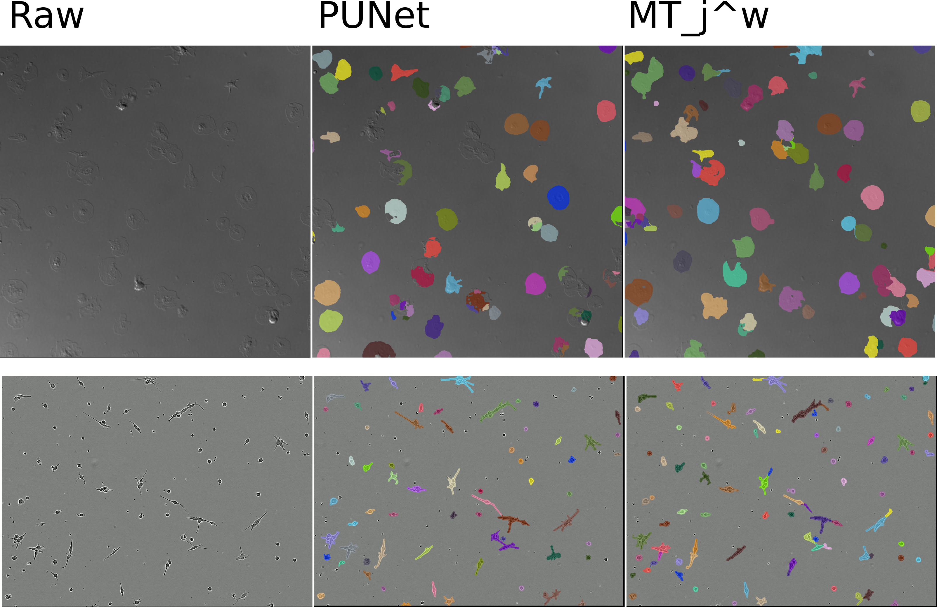
Figure 5: Instance segmentation results obtained from PUNet compared with $MT_{j}^{w}$ on two different images from the NeurIPS challenge held-out set. We observe that the semi-supervised model recovers more cells for the differential intensity contrast images (top row) and suffers less wrong merges (incorrect joining into one object of two or more cells) for the phase-contrast images (bottom row).

References

- [1] Berthelot, D., Carlini, N., Cubuk, E.D., Kurakin, A., Sohn, K., Zhang, H., Raffel, C.: ReMixMatch: Semi-Supervised Learning with Distribution Alignment and Augmentation Anchoring (Feb 2020), arXiv:1911.09785 [cs, stat]
- [2] Berthelot, D., Roelofs, R., Sohn, K., Carlini, N., Kurakin, A.: AdaMatch: A Unified Approach to Semi-Supervised Learning and Domain Adaptation (Mar 2022), arXiv:2106.04732 [cs]
- [3] Edlund, C., Jackson, T.R., Khalid, N., Bevan, N., Dale, T., Dengel, A., Ahmed, S., Trygg, J., Sjögren, R.: Livecell—a large-scale dataset for label-free live cell segmentation. Nature methods 18(9), 1038–1045 (2021)
- [4] Gerhard, S., Funke, J., Martel, J., Cardona, A., Fetter, R.: Segmented anisotropic sstem dataset of neural tissue. figshare pp. 0–0 (2013)
- [5] Jaeger, S., Candemir, S., Antani, S., Wáng, Y.X.J., Lu, P.X., Thoma, G.: Two public chest x-ray datasets for computer-aided screening of pulmonary diseases. Quantitative imaging in medicine and surgery 4(6), 475 (2014)
- [6] Kendall, A., Badrinarayanan, V., Cipolla, R.: Bayesian segnet: Model uncertainty in deep convolutional encoder-decoder architectures for scene understanding. arXiv preprint arXiv:1511.02680 (2015)
- [7] Kohl, S.A.A., Romera-Paredes, B., Maier-Hein, K.H., Rezende, D.J., Eslami, S.M.A., Kohli, P., Zisserman, A., Ronneberger, O.: A Hierarchical Probabilistic U-Net for Modeling Multi-Scale Ambiguities (May 2019). https://doi.org/10.48550/arXiv.1905.13077, http://arxiv.org/abs/1905.13077, arXiv:1905.13077 [cs]
- [8] Kohl, S.A.A., Romera-Paredes, B., Meyer, C., De Fauw, J., Ledsam, J.R., Maier-Hein, K.H., Eslami, S.M.A., Rezende, D.J., Ronneberger, O.: A Probabilistic U-Net for Segmentation of Ambiguous Images (Jan 2019), arXiv:1806.05034 [cs, stat]
- [9] Kohl, S.A., Romera-Paredes, B., Maier-Hein, K.H., Rezende, D.J., Eslami, S., Kohli, P., Zisserman, A., Ronneberger, O.: A hierarchical probabilistic u-net for modeling multi-scale ambiguities. arXiv preprint arXiv:1905.13077 (2019)
- [10] Lucchi, A., Li, Y., Smith, K., Fua, P.: Structured image segmentation using kernelized. In: Computer Vision–ECCV 2012: 12th European Conference on Computer Vision, Florence, Italy, October 7-13, 2012, Proceedings, Part II. vol. 7573, p. 400. Springer (2012)
- [11] Matskevych, A., Wolny, A., Pape, C., Kreshuk, A.: From shallow to deep: exploiting feature-based classifiers for domain adaptation in semantic segmentation. Front. Comput. Sci 4 (2022)
- [12] Mei, K., Zhu, C., Zou, J., Zhang, S.: Instance Adaptive Self-Training for Unsupervised Domain Adaptation (Aug 2020). https://doi.org/10.48550/arXiv.2008.12197, http://arxiv.org/abs/2008.12197, arXiv:2008.12197 [cs]
- [13] Ronneberger, O., Fischer, P., Brox, T.: U-net: Convolutional networks for biomedical image segmentation. In: Medical Image Computing and Computer-Assisted Intervention–MICCAI 2015: 18th International Conference, Munich, Germany, October 5-9, 2015, Proceedings, Part III 18. pp. 234–241. Springer (2015)
- [14] Sedai, S., Antony, B., Rai, R., Jones, K., Ishikawa, H., Schuman, J., Gadi, W., Garnavi, R.: Uncertainty guided semi-supervised segmentation of retinal layers in oct images. In: Medical Image Computing and Computer Assisted Intervention–MICCAI 2019: 22nd International Conference, Shenzhen, China, October 13–17, 2019, Proceedings, Part I 22. pp. 282–290. Springer (2019)
- [15] Shi, Y., Zhang, J., Ling, T., Lu, J., Zheng, Y., Yu, Q., Qi, L., Gao, Y.: Inconsistency-aware Uncertainty Estimation for Semi-supervised Medical Image Segmentation (Oct 2021), arXiv:2110.08762 [cs]
- [16] Shiraishi, J., Katsuragawa, S., Ikezoe, J., Matsumoto, T., Kobayashi, T., Komatsu, K.i., Matsui, M., Fujita, H., Kodera, Y., Doi, K.: Development of a digital image database for chest radiographs with and without a lung nodule: receiver operating characteristic analysis of radiologists’ detection of pulmonary nodules. American Journal of Roentgenology 174(1), 71–74 (2000)
- [17] Sohn, K., Berthelot, D., Li, C.L., Zhang, Z., Carlini, N., Cubuk, E.D., Kurakin, A., Zhang, H., Raffel, C.: FixMatch: Simplifying Semi-Supervised Learning with Consistency and Confidence (Nov 2020), arXiv:2001.07685 [cs, stat]
- [18] Sohn, K., Lee, H., Yan, X.: Learning structured output representation using deep conditional generative models. In: Cortes, C., Lawrence, N., Lee, D., Sugiyama, M., Garnett, R. (eds.) Advances in Neural Information Processing Systems. vol. 28. Curran Associates, Inc. (2015)
- [19] Tang, Y.B., Tang, Y.X., Xiao, J., Summers, R.M.: Xlsor: A robust and accurate lung segmentor on chest x-rays using criss-cross attention and customized radiorealistic abnormalities generation. In: International Conference on Medical Imaging with Deep Learning. pp. 457–467. PMLR (2019)
- [20] Tarvainen, A., Valpola, H.: Mean teachers are better role models: Weight-averaged consistency targets improve semi-supervised deep learning results (Apr 2018), arXiv:1703.01780 [cs, stat]
- [21] Wei, D., Lin, Z., Franco-Barranco, D., Wendt, N., Liu, X., Yin, W., Huang, X., Gupta, A., Jang, W.D., Wang, X., et al.: Mitoem dataset: Large-scale 3d mitochondria instance segmentation from em images. In: International Conference on Medical Image Computing and Computer-Assisted Intervention. pp. 66–76. Springer (2020)
- [22] Wolny, A., Yu, Q., Pape, C., Kreshuk, A.: Sparse Object-Level Supervision for Instance Segmentation With Pixel Embeddings. pp. 4402–4411 (2022)
- [23] Yang, L., Qi, L., Feng, L., Zhang, W., Shi, Y.: Revisiting Weak-to-Strong Consistency in Semi-Supervised Semantic Segmentation (Aug 2022), arXiv:2208.09910 [cs]
- [24] Yu, L., Wang, S., Li, X., Fu, C.W., Heng, P.A.: Uncertainty-aware Self-ensembling Model for Semi-supervised 3D Left Atrium Segmentation (Jul 2019), arXiv:1907.07034 [cs]
- [25] Yun, S., Han, D., Oh, S.J., Chun, S., Choe, J., Yoo, Y.: CutMix: Regularization Strategy to Train Strong Classifiers with Localizable Features (Aug 2019). https://doi.org/10.48550/arXiv.1905.04899, http://arxiv.org/abs/1905.04899, arXiv:1905.04899 [cs]
- [26] Zou, Y., Yu, Z., Kumar, B.V.K.V., Wang, J.: Domain Adaptation for Semantic Segmentation via Class-Balanced Self-Training (Oct 2018), arXiv:1810.07911 [cs]
- [27] Zou, Y., Zhang, Z., Zhang, H., Li, C.L., Bian, X., Huang, J.B., Pfister, T.: PseudoSeg: Designing Pseudo Labels for Semantic Segmentation (Mar 2021). https://doi.org/10.48550/arXiv.2010.09713, http://arxiv.org/abs/2010.09713, arXiv:2010.09713 [cs]