Skeleton Regression: A Graph-Based Approach to Estimation with Manifold Structure

Abstract

We introduce a new regression framework designed to deal with large-scale, complex data that lies around a low-dimensional manifold. Our approach first constructs a graph representation, referred to as the skeleton, to capture the underlying geometric structure. We then define metrics on the skeleton graph and apply nonparametric regression techniques, along with feature transformations based on the graph, to estimate the regression function. In addition to the included nonparametric methods, we also discuss the limitations of some nonparametric regressors with respect to the general metric space such as the skeleton graph. The proposed regression framework allows us to bypass the curse of dimensionality and provides additional advantages that it can handle the union of multiple manifolds and is robust to additive noise and noisy observations. We provide statistical guarantees for the proposed method and demonstrate its effectiveness through simulations and real data examples.

Keywords: manifold learning, nonparametric regression, kernel regression, spline

1 Introduction

Many data nowadays are geometrically structured that the covariates lie around a low-dimensional manifold embedded inside a large-dimensional vector space. Among many geometric data analysis tasks, the estimation of functions defined on manifolds has been extensively studied in the statistical literature. A classical approach to explicitly account for geometric structure takes two steps: map the data to the tangent plane or some embedding space and then run regression methods with the transformed data. This approach is pioneered by the Principle Component Regression (PCR) (Massy, 1965) and the Partial Least Squares (PLS) (Wold, 1975). Aswani et al. (2011) innovatively relate the regression coefficients to exterior derivatives. They propose to learn the manifold structure through local principal components and then constrain the regression to lie close to the manifold by solving a weighted least-squares problem with Ridge regularization. Cheng and Wu (2013) present the Manifold Adaptive Local Linear Estimator for the Regression (MALLER) that performs the local linear regression (LLR) on a tangent plane estimate. However, because those methods directly exploit the local manifold structures in an exact sense, they are not robust to variations in the covariates that perturb them away from the true manifold structure.

Many other manifold estimation approaches exist in the statistical literature. Guhaniyogi and Dunson (2016) utilize random compression of the feature vector in combination with Gaussian process regression. Zhang et al. (2013) follows a divide-and-conquer approach that computes an independent kernel Ridge regression estimator for each randomly partitioned subset. Other nonparametric regression approaches such as kernel machine learning (Schölkopf and Smola, 2002), manifold regularization (Belkin et al., 2006), and the spectral series approach (Lee and Izbicki, 2016) also account for the manifold structure of the data. However, those methods still suffer from the curse of dimensionality with large-dimensional covariates.

In addition to data with manifold-based covariates, manifold learning has been applied to other types of manifold-related data. Marzio et al. (2014) develop nonparametric smoothing for regression when both the predictor and the response variables are defined on a sphere. Zhang et al. (2019) deal with the presence of grossly corrupted manifold-valued responses. Green et al. (2021) proposes the Principal Components Regression with Laplacian-Eigenmaps (PCR-LE) that projects responses onto the eigenvectors output by Laplacian Eigenmaps. Lin and Yao (2020) address data with functional predictors that reside on a finite-dimensional manifold with contamination. In this work, we focus on manifold-based covariates and may incorporate other types of manifold-related data in the future.

The main goal of this work is to estimate scalar responses on manifold-structured covariates in a way that bypasses the curse of dimensionality. This is achieved by proposing a new framework that utilizes graphs and nonparametric regression techniques. Our framework follows the two-step idea: first, we learn a graph representation, which we call the skeleton, of the manifold structure based on the methods from Wei and Chen (2023) and project the covariates onto the skeleton. Then we apply different nonparametric regression methods to the skeleton-projected data. We give brief descriptions of the relevant nonparametric regression methods below.

Kernel smoothing is a widely used technique that estimates the regression function as locally weighted averages with the kernel as the weighting function. Pioneered by Nadaraya (1964) and Watson (1964) with the famous Nadaraya–Watson estimator, this technique has been widely used and extended by recent works (Fan and Fan (1992), Hastie and Loader (1993), Fan et al. (1996), Kpotufe and Verma (2017)). Splines (Hastie et al. (2009), Friedman (1991)) are popular nonparametric regression constructs that take the derivative-based measure of smoothness into account when fitting a regression function. Moreover, k-Nearest-Neighbors (kNN) regression (Altman, 1992; Hastie et al., 2009) has a simple form but is powerful and widely used in many applications. These techniques are incorporated into our proposed regression framework.

In recent years, many nonparametric regression techniques have been shown to adapt to the manifold structure of the data, with convergence rates that depend only on the intrinsic dimension of the data space. Specifically, the kNN regressor and the kernel regressor have been shown to be manifold-adaptive with proper parameter tuning procedures (Kpotufe, 2009, 2011; Kpotufe and Garg, 2013; Kpotufe and Verma, 2017). The proposed regression framework in this work also adapts to the manifold, as the nonparametric regression models fitted on a graph are dimension-independent. This framework has several additional advantages such as the ability to account for predictors from distinct manifolds and being robust to additive noise and noisy observations.

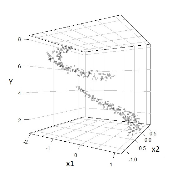
(a) Data

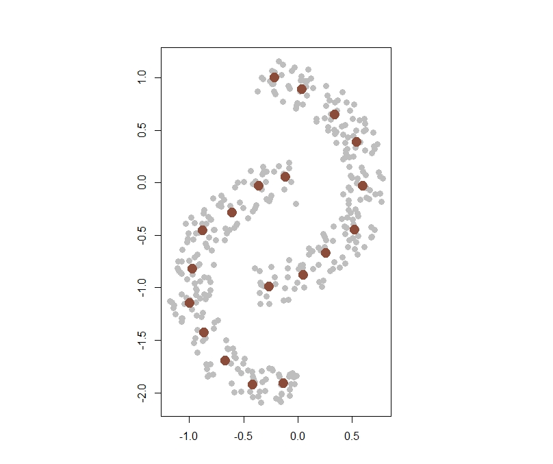
(b) Knots

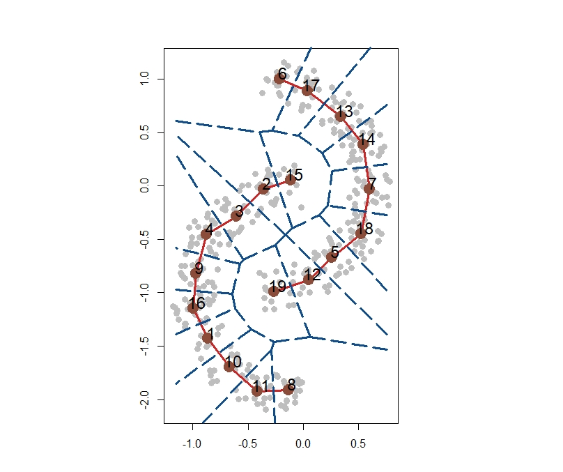
(c) Skeleton

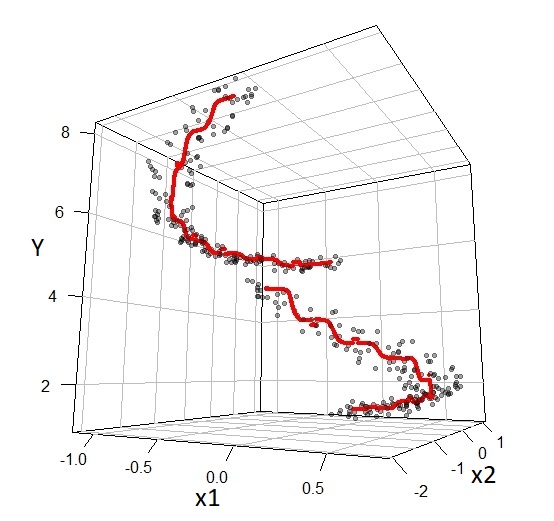
(d) S-Kernel Regression

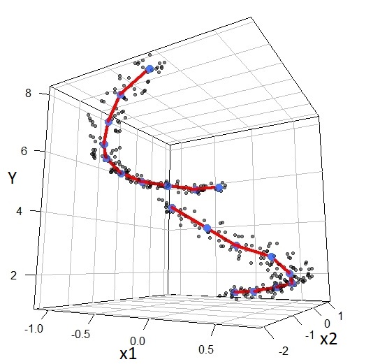
(e) Linear Spline

Figure 1: Skeleton Regression illustrated by Two Moon Data (d=2).

Outline. We start by presenting the procedures of the skeleton regression framework in section 2. In section 3, we apply nonparametric regression techniques to the constructed skeleton graph along with theoretical justifications. In section 4, we present some simulation results for skeleton regression and demonstrate the effectiveness of our method on real datasets in Section 5. In section 6, we conclude the paper and point out some directions for future research.

2 Skeleton Regression Framework

In this section, we introduce the skeleton regression framework. Given design vectors $\left\{\bm{x}_{i}\right\}_{i=1}^{n}$ where $\bm{x}_{i}\in{\mathcal{X}}\subseteq{\mathbb{R}}^{d}$ for each $i$ and the corresponding responses $\left\{Y_{i}\right\}_{i=1}^{n}$ in ${\mathbb{R}}$, a traditional regression approach is to estimate the regression function $m(\bm{x})={\mathbb{E}}(Y|X=\bm{x})$. However, the ambient dimension $d$ can be large while the covariates are distributed on a low-dimensional manifold structure. In this case, ${\mathcal{X}}$ can be the union of several disjoint components with different manifold structures, and the regression function can have discontinuous changes from one component to another. To handle such manifold-structured data, we approach the regression task by first representing the sample covariate space with a graph, which we call the skeleton, to summarize the manifold structures. We then focus on the regression function over the skeleton graph, which incorporates the covariate geometry in a dimension-independent way.

We illustrate our regression framework on simulated TwoMoon data in Figure 1. The covariates of the TwoMoon data consist of two $2$-dimensional clumps with intrinsically 1-dimensional curve structure, and the regression response increases polynomially with the angle and the radius (Figure 1 (a)). We construct the skeleton presentation to summarize the geometric structure (Figure 1 (b,c) ) and project the covariates onto the skeleton. The regression function on the skeleton is estimated using kernel smoothing (Section 3.1, illustrated in Figure 1 (d) ) and linear spline (Section 3.3, illustrated in Figure 1 (e)). The estimated regression function can be used to predict new projected covariates. We summarize the overall procedure in Algorithm 1.

Algorithm 1 Skeleton Regression

Input: Observations $(\bm{x}_{1},Y_{1}),\dots,(\bm{x}_{n},Y_{n})$.

1. Skeleton Construction. Construct a data-driven skeleton representation of the covariates preferably assisted with subject knowledge.

2. Data Projection. Project the covariates onto the skeleton.

3. Skeleton Regression Function Estimation. Fitting regression function on the skeleton using nonparametric techniques such as kernel smoothing (Section 3.1), k-Nearest Neighbor (Section 3.2), and linear spline (Section 3.3).

4. Prediction. Project new covariates onto the skeleton and use the estimated regression function for prediction.

2.1 Skeleton Construction

A skeleton is a low-dimensional subset of the sample space representing regions of interest that admits a graph representation. For given covariate space ${\mathcal{X}}\subseteq{\mathbb{R}}^{d}$, let ${\mathcal{V}}=\{V_{j}\in{\mathbb{R}}^{d}:j=1,\dots k\}$ be a collection of points of interest and $E$ be a set of edges connecting points in ${\mathcal{V}}$ such that an edge $e_{j\ell}\in E$ if the region between $V_{j}$ and $V_{\ell}$ is also of interest. The tuple $({\cal V},E)$ together forms a graph that represents the focused regions in the sample space. Notably, different from common graph-based regression approaches that take each sample covariate as a vertex, the set ${\mathcal{V}}$ takes representative points of the covariate space and has size $k\ll n$ where $n$ is the sample size. Moreover, the points on the edges are also part of the analysis as belonging to the regions of interest, which is different from the usual knot-edge graph. While the graph $({\cal V},E)$ contains the region of interest, it is not easy to work with this graph directly. Thus, we introduce the concept of the skeleton induced by this graph.

Let ${\mathcal{E}}=\{tV_{j}+(1-t)V_{\ell}:t\in(0,1),e_{j\ell}\in E\}$ be the collection of line segments induced by the edge set $E$. We define the skeleton of $({\cal V},E)$ as ${\mathcal{S}}={\mathcal{V}}\cup{\mathcal{E}}$, i.e., ${\mathcal{S}}$ is the points of interest and the associated line segments representing the regions of interest. Clearly, ${\mathcal{S}}$ is a collection of one-dimensional line segments and zero-dimensional points so it is independent of the ambient dimension $d$, but the physical location of ${\mathcal{S}}$ is meaningful as representing the region of interest. The idea of skeleton regression is to build a regression model on the skeleton ${\mathcal{S}}$.

2.1.1 A data-driven approach to construct skeleton

The skeleton should ideally be constructed based on the analyst’s judgment or prior knowledge of the region of interest. However, this information may be unavailable and we have to construct a skeleton from the data. In this section, we give a brief description of a data-driven approach proposed in Wei and Chen (2023) that constructs the skeleton to represent high-density regions. The method constructs knots as the centers from the $k$-means clustering with a large number of knots . The edges are connected by examining the sample 2-Nearest-Neighbor (2-NN) region of a pair of knots $(V_{j},V_{\ell})$ (see Figure 2)

$$B_{j\ell}=\{X_{m},m=1,\dots,n:\left\|x-V_{i}\right\|>\max\{\left\|x-V_{j}\right\|,\left\|x-V_{\ell}\right\|\},\forall i\neq j,\ell\},$$ (1)

where $||.||$ denotes the Euclidean norm, and an edge between $V_{j}$ and $V_{\ell}$ is added if $B_{j\ell}$ is non-empty. The method can further prune edges or segment the skeleton by using hierarchical clustering with respect to the Voronoi Density weights defined as $S_{j\ell}^{VD}=\frac{\frac{1}{n}\left|B_{j\ell}\right|}{\left\|V_{j}-V_{\ell}\right\|}.$ We provide more details about this approach in Appendix A.

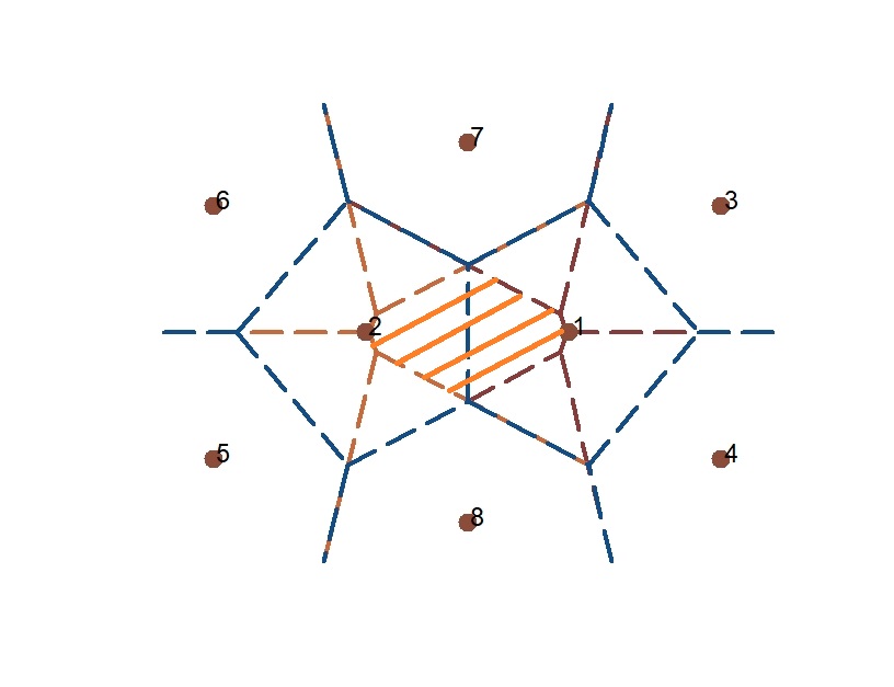
Figure 2: Orange shaded area illustrates the 2-NN region of knots $1,2$.

Remark 1

The idea of using the $k$-means algorithm to divide data into cells and perform analysis based on the cells has been proposed in the literature for fast computation. Sivic and Zisserman (2003), when carrying out an approximate nearest neighbor search, proposed to divide the data into Voronoi cells by $k$-means and do a neighbor search only in the same or some nearby cells. Babenko and Lempitsky (2012) adopted the Product Quantization technique to construct cell centers for high-dimensional data as the Cartesian product of centers from sub-dimensions.

2.2 Skeleton-Based Distance

One of the advantages of the physically-located skeleton is that it allows for a natural definition of the skeleton-based distance function $d_{\mathcal{S}}(.,.):{\mathcal{S}}\times{\mathcal{S}}\to{\mathbb{R}}^{+}\cup\{\infty\}$. Let $\bm{s}_{j},\bm{s}_{\ell}\in{\mathcal{S}}$ be two arbitrary points on the skeleton and note that, different from the usual geodesic distance on a graph, in our framework $\bm{s}_{j},\bm{s}_{\ell}$ can be on the edges. We measure the skeleton-based distance between two skeleton points as the graph path length as defined below:

• If $\bm{s}_{j},\bm{s}_{\ell}$ are disconnected that they belong to two disjoint components of ${\mathcal{S}}$, we define

  $$d(\bm{s}_{j},\bm{s}_{\ell})=\infty$$ (2)

• If $\bm{s}_{j}$ and $\bm{s}_{\ell}$ are on the same edge, we define the skeleton distance as their Euclidean distance that

  $$d_{\mathcal{S}}(\bm{s}_{j},\bm{s}_{\ell})=||\bm{s}_{j}-\bm{s}_{\ell}||$$ (3)

• For $\bm{s}_{j}$ and $\bm{s}_{\ell}$ on two different edges that share a knot $V_{0}$, the skeleton distance is defined as

  $$d_{\mathcal{S}}(\bm{s}_{j},\bm{s}_{\ell})=||\bm{s}_{j}-V_{0}||+||\bm{s}_{\ell}-V_{0}||$$ (4)

• Otherwise, let knots $V_{i(1)},\dots,V_{i(m)}$ be the vertices on a path connecting $\bm{s}_{j},\bm{s}_{\ell}$, where $V_{i(1)}$ is one of the two closest knots of $\bm{s}_{j}$ and $V_{i(m)}$ is the other closest knots of $\bm{s}_{\ell}$. We add the edge lengths of the in-between knots to the distance that

  $$\begin{split}d_{\mathcal{S}}(\bm{s}_{j},\bm{s}_{\ell})&=||\bm{s}_{j}-V_{i(1)}||+||\bm{s}_{\ell}-V_{i(m)}||+\sum_{p=1}^{m-1}\left\|V_{i(p)},V_{i(p+1)}\right\|\end{split}$$ (5)

  and we use the shortest path length if there are multiple paths connecting $\bm{s}_{j}$ and $\bm{s}_{\ell}$.

An example illustrating the skeleton-based distance is shown in Figure 3. Like the shortest path (geodesic) distance that makes a usual knot-edge graph into a metric space, the skeleton-based distance is also a metric on the skeleton graph. In the following sections, we will discuss methods to perform regression on space only with the defined metric.

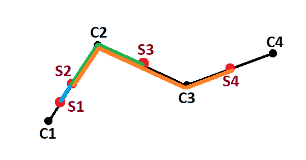
Figure 3: Illustration of skeleton-based distance. Let $C_{1},C_{2},C_{3},C_{4}$ be the knots, and let $S_{2},S_{3},S_{4}$ be the mid-point on the edges $E_{12},E_{23},E_{34}$ respectively. Let $S_{1}$ bet the midpoint between $C_{1}$ and $S_{2}$ on the edge. Let $d_{ij}=\left\|C_{i}-C_{j}\right\|$ denotes the length of the edge $E_{ij}$. $d_{\mathcal{S}}(S_{1},S_{2})=\frac{1}{4}d_{12}$ illustrated by the blue path. $d_{\mathcal{S}}(S_{2},S_{3})=\frac{1}{2}d_{12}+\frac{1}{2}d_{23}$ illustrated by the green path. $d_{\mathcal{S}}(S_{2},S_{4})=\frac{1}{2}d_{12}+d_{23}+\frac{1}{2}d_{34}$ illustrated by the orange path.

Remark 2

We may view the skeleton-based distance as an approximation of the geodesic distance on the underlying data manifold. Moreover, to make a stronger connection to the manifold structure, it is possible to define edge lengths through local manifold learning techniques that have better approximations to the local manifold structure. However, using more complex local edge weights can pose additional challenges for the data projection step described in the next section and we leave this as a future direction.

2.3 Data Projection

For the next step, we project the sample covariates onto the constructed skeleton. For given covariate $\bm{x}$, let $I_{1}(\bm{x}),I_{2}(\bm{x})\in\{1,\dots,k\}$ be the index of its closest and second closest knots in terms of the Euclidean metric. We define the projection function $\Pi(.):{\mathcal{X}}\to{\mathcal{S}}$ for $\bm{x}\in{\mathcal{S}}$ as (illustrated in Figure 4):

• If $V_{I_{1}(\bm{x})}$ and $V_{I_{2}(\bm{x})}$ are not connected, $\bm{x}$ is projected onto the closest knot that $\Pi(\bm{x})=V_{I_{1}(\bm{x})}$

• If $V_{I_{1}(\bm{x})}$ and $V_{I_{2}(\bm{x})}$ are connected, $\bm{x}$ is projected with the Euclidean metric onto the line passing through $V_{I_{1}(\bm{x})}$ and $V_{I_{2}(\bm{x})}$ that, let $t=\frac{\left(\bm{x}-V_{I_{1}(\bm{x})}\right)^{T}\cdot\left(V_{I_{2}(\bm{x})}-V_{I_{1}(\bm{x})}\right)}{\left\|V_{I_{2}(\bm{x})}-V_{I_{1}(\bm{x})}\right\|^{2}}$ be the projection proportion,

  $$\Pi(\bm{x})=V_{I_{1}(\bm{x})}+\left(V_{I_{2}(\bm{x})}-V_{I_{1}(\bm{x})}\right)\cdot\begin{cases}0,\text{ if }t<0\\ 1,\text{ if }t>1\\ t,\text{ otherwise}\end{cases}$$ (6)

  where we constrain the covariates to be projected onto the closest edge.

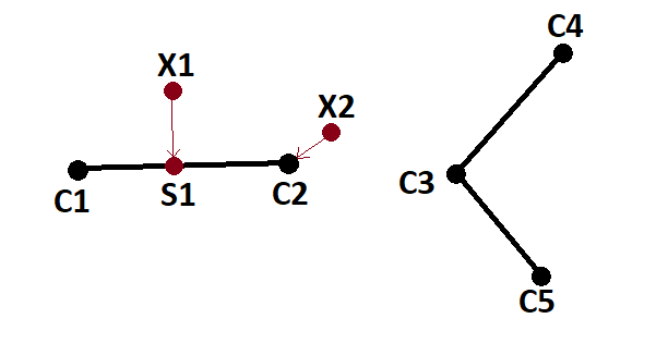
Figure 4: Illustration of projection to the skeleton. The skeleton structure is given by the black dots and lines. Data point $X_{1}$ is projected to $S_{1}$ on the edge between $C_{1}$ and $C_{2}$. Data point $X_{2}$ is projected to knot $C_{2}$.

Note that with the projection defined above, a non-trivial volume of points can be projected onto the end knots of the skeleton graph as belonging to Case I or due to the constraining in Case II. This adds complexities to the theoretical analysis of the proposed regression framework and leads to our separate analysis of the different domains of the graph in Section 3.1.1.

3 Skeleton Nonparametric Regression

Covariates are mapped to locations on the skeleton after the data projection step and are equipped with the skeleton-based distances. In this section, we apply nonparametric regression techniques to the skeleton graph with projected data points. We study three feasible nonparametric approaches: the skeleton-based kernel regression (S-Kernel), the skeleton-based k-nearest-neighbor method (S-kNN), and the linear spline model (S-Lspline). At the end of this section, we discuss the challenges of applying some other nonparametric regression methods in the setting of skeleton graph.

3.1 Skeleton Kernel Regression

We start by adopting kernel smoothing to the skeleton graph. Let $\bm{s}_{1},\cdots,\bm{s}_{n}$ be the projections on the skeleton from $\bm{x}_{1},\cdots,\bm{x}_{n}$, i.e., $\bm{s}_{i}=\Pi(\bm{x}_{i})$. With the skeleton-based distances, the skeleton kernel regression makes a prediction at the location $\bm{s}\in{\mathcal{S}}$ as

$$\hat{m}(\bm{s})=\frac{\sum_{i=1}^{N}K(d_{\mathcal{S}}(\bm{s}_{i},\bm{s})/h)Y_{i}}{\sum_{j=1}^{N}K(d_{\mathcal{S}}(\bm{s}_{j},\bm{s})/h)},$$ (7)

where $K(\cdot)\geq 0$ is a smoothing kernel such as the Gaussian kernel and $h>0$ is the smoothing bandwidth that controls the amount of smoothing. In practice, we choose $h$ by cross-validation. Essentially, the estimator $\hat{m}(\bm{s})$ is the usual kernel regression applied to a general metric space (skeleton) rather than the usual Euclidean space. Notably, the kernel function calculation only depends on the skeleton distances and hence is independent of neither the ambient dimension of the original input nor the intrinsic dimension of the manifold structure.

It should be also noted that $\hat{m}(\bm{s})$ only makes prediction on $\bm{s}\in{\mathcal{S}}$. If we are interested in predicting the outcome at any arbitrary point $\bm{x}\in{\mathcal{X}}$, the prediction will be based on the projected point, i.e., $\hat{m}(\bm{x})=\hat{m}\left(\Pi(\bm{x})\right),$ where $\Pi(\bm{x})\in{\mathcal{S}}.$ Because of the above projection property, one can think of the skeleton kernel regression as an estimator to the following skeleton-projected regression function

$$m_{\mathcal{S}}(\bm{s})={\mathbb{E}}(\bm{Y}|\Pi(\bm{X})=\bm{s}),\bm{s}\in{\mathcal{S}}.$$ (8)

We study the convergence of $\hat{m}(\bm{s})$ to $m_{\mathcal{S}}(\bm{s})$ in what follows.

3.1.1 Consistency of S-Kernel Regression

Our analysis assumes that the skeleton is fixed and given and focuses on the estimation of the regression function. To evaluate the estimation error, we must first impose some concepts of distribution on the skeleton. However, due to the covariate projection procedure, the probability measures on the knots and edges are different. Therefore, we analyze them separately. On an edge, the domain of the projected regression function varies in one dimension, resulting in a standard univariate problem for estimation. For the case of knots, a nontrivial region of the covariate space can be projected onto a knot, leading to a nontrivial probability mass at the knot.

For simplicity, we write $K_{h}(\bm{s}_{j},\bm{s}_{\ell})\equiv K(d_{\mathcal{S}}(\bm{s}_{j},\bm{s}_{\ell})/h)$ for $\bm{s}_{j},\bm{s}_{\ell}\in{\mathcal{S}}$. Let ${\mathcal{B}}(\bm{s},h)=\left\{\bm{s}^{\prime}\in{\mathcal{S}}:d_{\mathcal{S}}(\bm{s}^{\prime},\bm{s})<h\right\}$ be the ball on skeleton centered at the point $\bm{s}\in{\mathcal{S}}$ with radius $h$. We can decompose the kernel regression estimator into edge parts and knot parts as

$$\begin{split}\hat{m}(\bm{s})&=\frac{\sum_{j=1}^{n}Y_{j}K_{h}(\bm{s}_{j},\bm{s})}{\sum_{j=1}^{n}K_{h}(\bm{s}_{j},\bm{s})}\\ &=\frac{\frac{1}{n}\sum_{j=1}^{n}Y_{j}K_{h}(\bm{s}_{j},\bm{s})I(\bm{s}_{j}\in{\mathcal{E}})+\frac{1}{n}\sum_{j=1}^{n}Y_{j}K_{h}(\bm{s}_{j},\bm{s})I(\bm{s}_{j}\in{\mathcal{V}})}{\frac{1}{n}\sum_{j=1}^{n}K_{h}(\bm{s}_{j},\bm{s})I(\bm{s}_{j}\in{\mathcal{E}})+\frac{1}{n}\sum_{j=1}^{n}K_{h}(\bm{s}_{j},\bm{s})I(\bm{s}_{j}\in{\mathcal{V}})}\\ &=\frac{\frac{1}{n}\sum_{j=1}^{n}Y_{j}K_{h}(\bm{s}_{j},\bm{s})I(\bm{s}_{j}\in{\mathcal{E}}\cap{\mathcal{B}}(\bm{s},h))+\frac{1}{n}\sum_{j=1}^{n}Y_{j}K_{h}(\bm{s}_{j},\bm{s})I(\bm{s}_{j}\in{\mathcal{V}}\cap{\mathcal{B}}(\bm{s},h))}{\frac{1}{n}\sum_{j=1}^{n}K_{h}(\bm{s}_{j},\bm{s})I(\bm{s}_{j}\in{\mathcal{E}}\cap{\mathcal{B}}(\bm{s},h))+\frac{1}{n}\sum_{j=1}^{n}K_{h}(\bm{s}_{j},\bm{s})I(\bm{s}_{j}\in{\mathcal{V}}\cap{\mathcal{B}}(\bm{s},h))}\end{split}$$ (9)

In the last line, we emphasize that the knots and edges in the kernel estimator have a meaningful contribution only within the support of the kernel function. We inspect the different domain cases separately in the following sections.

For the model and assumptions, we let $Y_{j}=m_{\mathcal{S}}(\bm{S}_{j})+U_{j},\bm{S}_{j}\in{\mathcal{S}}$, and ${\mathbb{E}}(U_{j}|\bm{S}_{j})=0$ almost surely. Let $\sigma^{2}(\bm{s})={\mathbb{E}}(U_{j}^{2}|\bm{S}_{j}=\bm{s})$. Let the density on the skeleton edge be defined as the 1-Hausdorff density that $g(\bm{s})=\lim_{r\downarrow 0}\frac{P(\bm{S}\in{\mathcal{B}}(\bm{s},r))}{2r}$. Note that $g(\bm{s})=\infty$ if $\bm{s}$ is at a knot point that has a probability mass. We consider the following assumptions:

• $\sigma^{2}(\bm{s})$ is continuous and uniformly bounded.

• The skeleton edge density function $g(\bm{s})>0$ and are bounded and Lipschitz continuous for $\bm{s}\in{\mathcal{E}}$.

• $m_{\mathcal{S}}(\bm{s})g(\bm{s})$ is bounded and Lipschitz continuous for $\bm{s}\in{\mathcal{E}}$.

• The kernel function has compact support and satisfies $\int K(x)dx=1$, $\int K^{2}(x)dx<\infty$, $\int xK(x)dx=0$, and $\int x^{2}K(x)dx<\infty$

Conditions A1 and K are general assumptions that are commonly made in kernel regression analysis. A2 and A3 are mild conditions that can be sufficiently implied by the boundedness and Lipschitz continuity of the density and regression function in the ambient space along with non-overlapping knots that the area of the orthogonal complements have Lipschitz changes. We do not assume the second-order smoothness commonly required for kernel regression because requiring higher-order derivative smoothness would necessitate specifying directions on the graph, which may present difficulties in model formulation. We include further discussions about derivatives on the skeleton in Section 3.4.

3.1.2 Convergence of the Edge Point

We first look at an edge point $\bm{s}\in E_{j\ell}\in{\mathcal{E}}$. In this case, as $n\to\infty,h\to 0$, for sufficiently large $n$, we have ${\mathcal{B}}(\bm{s},h)\subset E_{j\ell}$, and the skeleton distance is the $1$-dimensional Euclidean distance for any point within the support. Therefore, we have a convergence rate similar to the $1$-dimensional kernel regression estimator (Bierens, 1983; Wasserman, 2006; Chen, 2017).

Theorem 1 (Consistency on Edge Points)

For $\bm{s}\in{\mathcal{E}}$ an edge point, assume conditions A1-3 and K hold for all points in ${\mathcal{E}}\cap{\mathcal{B}}(\bm{s},h)$, as $n\to\infty$, $h\rightarrow 0$, $nh\rightarrow\infty$,

$$\left|\hat{m}_{n}(\bm{s})-m_{\mathcal{S}}(\bm{s})\right|=O(h)+O_{p}\bigg{(}\sqrt{\frac{1}{nh}}\bigg{)}$$ (10)

We leave the proof in Appendix C.1. Theorem 1 gives the convergence rate for a point on the edge of the constructed skeleton. The convergence rate at the bias is $O(h)$, which is the usual rate when we only have Lipschitz smoothness (A2) of $m_{{\mathcal{S}}}$. One may be wondering if we can obtain a faster rate such as $O(h^{2})$ if we assume higher-order smoothness of $m_{{\mathcal{S}}}$. While it is possible to obtain a faster rate if we have a higher-order smoothness, this assumption will not be reasonable because $m_{\bm{S}}(\bm{s})={\mathbb{E}}(Y|\Pi(X)=\bm{s})$ is defined via a project. The region being projected onto $\bm{s}$ is continuously changing and may not be differentiable due to the boundary of Voronoi cells. Therefore, the Lipschitz continuity (A2) is reasonable while higher-order smoothness is not.

3.1.3 Convergence of the Knots with Nonzero Mass

We then look at the knots with nonzero probability mass that $\bm{s}\in{\mathcal{V}}$ with $p(\bm{s})>0$, where we use $p(\bm{s})$ to denote the probability mass on a knot. This case mainly occurs for knots with degree $1$ on the skeleton graph, when a non-trivial region of points is projected onto such knots. For example, refer to knot C2 in Figure 4.

Theorem 2 (Consistency on Knots with Nonzero Mass)

For $\bm{s}\in{\mathcal{V}}$ a knot point, let the probability mass at $\bm{s}$ be $P(\Pi_{\mathcal{S}}(X)=\bm{s})\equiv p(\bm{s})>0$ and assume $\sigma^{2}(\bm{s})$ bounded. Also assume conditions A1-3 and K hold for all edge points in ${\mathcal{E}}\cap{\mathcal{B}}(\bm{s},h)$. We have, as $n\to\infty$, $h\rightarrow 0$, and $nh\rightarrow\infty$,

$$\left|\hat{m}(\bm{s})-m_{\mathcal{S}}(\bm{s})\right|=O(h)+O_{p}\left(\sqrt{\frac{1}{n}}\right)$$ (11)

Theorem 2 gives the convergence result for a knot point with a nontrivial mass of the skeleton. The bias term $O(h)$ comes from the influence of nearby edge points. For the stochastic variation part, instead of having the $O_{p}\left(\sqrt{\frac{1}{nh}}\right)$ rate as the usual kernel regression and in Theorem 1, we have $O_{p}\left(\sqrt{\frac{1}{n}}\right)$ rate which comes from averaging the observations projected onto the knots. The proof of Theorem 2 is provided in Appendix C.3.

3.1.4 Convergence of the Knots with Zero Mass

We now look at a knot point $\bm{s}\in{\mathcal{V}}$ with no probability mass that $p(\bm{s})=0$. This is can be the case for a knot with a degree larger than $1$ like knot C3 in Figure 4. Since we define edge sets excluding the knots, there will be no density as well as no probability mass at $\bm{s}$. Note that, with some reformulation, degree $2$ knots can be parametrized together with the two connected edges and, under the appropriate assumptions, Theorem 1 applies, giving consistency estimation with $O(h)+O_{p}\left(\sqrt{\frac{1}{nh}}\right)$ rate. However, density cannot be extended directly to knots with a degree larger than $2$, but the kernel estimator still converges to some limits as presented in the Proposition below.

Proposition 3

For $\bm{s}\in{\mathcal{V}}$ a knot point, assume conditions A1-3 hold for all points in ${\mathcal{E}}\cap{\mathcal{B}}(\bm{s},h)$ and let the probability mass at $\bm{s}$ be $p(\bm{s})=0$. We assume condition K for the kernel function. Let ${\mathcal{I}}$ collect the indexes of edges with one knot being $\bm{s}$. For $\ell\in{\mathcal{I}}$ and edge $E_{\ell}$ connects $\bm{s}$ and $V_{\ell}$, let $g_{\ell}(t)=g((1-t)\bm{s}+tV_{\ell})$ and $g_{\ell}(0)=\lim_{x\downarrow 0}g_{\ell}(x)$. Let $m_{\ell}(t)=m_{\mathcal{S}}((1-t)\bm{s}+tV_{\ell})$ and $m_{\ell}(0)=\lim_{t\downarrow 0}m_{\ell}(t)$. We have, as $n\to\infty$, $h\rightarrow 0$, and $nh\rightarrow\infty$,

$$\hat{m}(\bm{s}) =\frac{\sum_{\ell\in{\mathcal{I}}}m_{\ell}(0)g_{\ell}(0)}{\sum_{\ell\in{\mathcal{I}}}g_{\ell}(0)}+O(h)+O_{p}\left(\sqrt{\frac{1}{nh}}\right).$$ (12)

Proposition 3 shows that, under proper conditions, the skeleton kernel estimator on a zero-mass knot converges to the weighted average of the limiting regression values of the connected edges, and the convergence rate is the same as the edge points shown in Theorem 1. The proof is included in Appendix C.2.

Remark 3

The domain ${\mathcal{S}}$ of the regression function can be seen as bounded, and hence the boundary bias issue can arise. The true manifold structure’s boundary can be different from the boundary of the skeleton graph, making the consideration of the boundary more complicated. However, the boundary of the skeleton is the set of degree $1$ knots, and, under our formulation, knots have discrete measures, so the consideration of boundary bias may not be necessary for the proposed formulation. However, some boundary corrections can potentially improve the empirical performance and we leave it for future research.

3.2 Skeleton kNN regression

The $k$-Nearest Neighbor (kNN) method can be easily applied to the skeleton using the distance on the skeleton. For a given point on the skeleton at $\bm{s}\in{\mathcal{S}}$, we define the distance to the k-th nearest observation on the skeleton as

$$R_{k}(\bm{s})=\min\left\{r>0:\sum_{i=1}^{n}I(d_{\mathcal{S}}(\bm{s}_{i},\bm{s})\leq r)\geq k\right\}.$$ (13)

Note that it is possible to have multiple observations being the $k$-th nearest observation due to observations being projected to the vertices. In this case, we can either randomly choose from them or consider all of them. Here we include all of them in the calculation. The skeleton-based $k$NN regression (S-kNN) predicts the value of outcome at $\bm{s}$ as

$$\hat{m}_{SkNN}(\bm{s})=\frac{\sum_{i=1}^{k}Y_{i}I(d_{\mathcal{S}}(\bm{s}_{i},\bm{s})\leq R_{k}(\bm{s}))}{\sum_{j=1}^{k}I(d_{\mathcal{S}}(\bm{s}_{j},\bm{s})\leq R_{k}(\bm{s}))}.$$ (14)

Different from the usual kNN regressor with the covariates $\bm{x}_{1},\dots,\bm{x}_{n}$, which selects neighbors through Euclidean distance in the ambient space, the S-kNN regressor chooses neighbors with skeleton-based distances after projection onto the skeleton graph. Measuring proximity with the skeleton can improve the regression performance when the dimension of the covariates is large, which we empirically show in Section 4.

Remark 4

It is well known that the usual $k_{n}$NN regressor can be consistent if we let $k_{n}$ grow as a function of the sample size $n$, and under appropriate assumptions, Györfi et al. (2002) give the convergence rate of the $k_{n}$NN estimate $m_{n}$ to the true function $m$ as

$$\mathbb{E}\left\|m_{n}-m\right\|^{2}\leq\frac{\sigma^{2}}{k_{n}}+c_{1}\cdot C^{2}\left(\frac{k_{n}}{n}\right)^{2/d}$$

Later, Kpotufe (2011) has shown that the convergence rate of $k$NN regressor depends on the intrinsic dimension. We expect a similar result with $d=1$ rate for the skeleton $k$NN regression at an edge point.

3.3 Linear Spline Regression on Skeleton

In this section, we propose a skeleton-based linear spline model (S-Lspline) for regression estimation. By construction, this approach results in a continuous model across the graph. Moreover, we show that the skeleton-based linear spline corresponds to an elegant parametric regression model on the skeleton. As the skeleton ${\mathcal{S}}$ can be decomposed into the edge component $\mathcal{E}$ and the knot component $\mathcal{V}$, the linear spline regression on the skeleton can be written as the following constrained model:

$$f:{\mathcal{S}}\,\,\rightarrow\,\,\mathbb{R}\ \ \mbox{ such that } f(x) x\in\mathcal{E}$$ 1. is linear on , (15)

2. $$f(x) x\in\mathcal{V}$$ is continuous at .

While solving the above constrained problem may not be easy, we have the following elegant representer theorem showing that a linear spline on the skeleton can be uniquely characterized by the values on each knot.

Theorem 5 (Linear spline representer theorem)

Any function satisfying equation (15) can be characterized by $\{f(v):v\in\mathcal{V}\}$ and for $x\in\mathcal{E}$, $f(x)$ is linear interpolation between the values on the two knots on the edge that $x$ belongs to.

Proof  Let $f$ be a function satisfying equation (15). By construct, $f$ is linear for $x\in{\mathcal{E}}$ and is continuous at $x\in{\mathcal{V}}$. Let $V_{j}$ and $V_{\ell}$ be two knots that share an edge and let $E_{j\ell}=\{x=tV_{j}+(1-t)V_{\ell}:t\in(0,1)\}$ be the shared edge segment. For any $x\in{\mathcal{E}}$, there exists a pair $(V_{j},V_{\ell})$ such that $x\in E_{j\ell}$. Because $f$ is linear in $E_{j\ell}$, $f$ can bee uniquely characterized by the pairs $(f(e_{1}),e_{1}),(f(e_{2}),e_{2})$ for two distinct points $e_{1},e_{2}\in\bar{E}_{j\ell}$, where $\bar{E}_{j\ell}=\{x=tV_{j}+(1-t)V_{\ell}:t\in[0,1]\}$ is the closure of $E_{j\ell}.$ Thus, we can pick $e_{1}=V_{j}$ and $e_{2}=V_{\ell}$, which implies that $f$ on the segment $E_{j\ell}$ is parameterized by $f(v_{j})$ and $f(V_{\ell})$, the values on the two knots.

By applying this procedure to every edge segment, we conclude that any function satisfying the first condition in (15) can be characterized by the values on the knots. The second condition in (15) will require that every knot has one consistent value. As a result, any function $f$ satisfying (15) can be uniquely characterized by the values on the knot $\{f(x):x\in{\mathcal{V}}\}$ and $f(x)$ will be a linear interpolation when $x\in{\mathcal{E}}$.

 

Using Theorem 5, we only need to determine the values on the knots. Let $\bm{\beta}\in\mathbb{R}^{k}$ be the values of skeleton linear spline model on each knot with $k=\left|{\mathcal{V}}\right|$ being the number of knots. As is argued previously, the spline model is parameterized by $\bm{\beta}$, so we only need to estimate $\bm{\beta}$ from the data. Given $\bm{\beta}$, the predicted value of each $\bm{y}_{i}$ is a linear interpolation depending on the projected location of each $\bm{x}_{i}$.

To derive an analytic form of $\bm{y}_{i}$, we introduce a transformed covariate matrix $\bm{Z}=(\bm{z}_{1},\dots,\bm{z}_{n})^{T}\in\bm{R}^{n\times k}$ as follows:

1. If $\bm{x}_{i}$ is projected onto a vertex that $\bm{s}_{i}=V_{j}$ for some $j$, then

   $$\bm{z}_{ij^{\prime}}=I(j^{\prime}=j).$$ (16)

2. If $\bm{x}_{i}$ is projected onto an edge between knots $V_{j}$ and $V_{\ell}$, then

   $$\bm{z}_{ij}=\frac{||\bm{s}_{i}-V_{j}||}{||V_{j}-V_{\ell}||},\quad\bm{z}_{i\ell}=\frac{||\bm{s}_{i}-V_{\ell}||}{||V_{j}-V_{\ell}||},\quad\text{ and }\bm{z}_{ij^{\prime}}=0\text{ for }j^{\prime}\neq j,\ell.$$ (17)

With the above feature transform, the predicted value of $\bm{y}_{i}$ by the S-Lspline model is

$$\hat{\bm{y}}_{i}=\bm{\beta}^{T}\bm{z}_{i}.$$ (18)

To see this, if $\bm{x}_{i}$ is projected onto a vertex that $\bm{s}_{i}=V_{j}$ for some $j$, the linear model with transformed covariates gives $\bm{\beta}^{T}\bm{z}_{i}=\bm{\beta}_{j}$, the predicted value on vertex $V_{j}$. In the case where $\bm{x}_{i}$ is projected onto an edge between knots $V_{j}$ and $V_{\ell}$, let $\bm{\beta}_{j}$ and $\bm{\beta}_{\ell}$ be the corresponding predicted values at $V_{j}$ and $V_{\ell}$, and the linear interpolation between $\bm{\beta}_{\ell}$ and $\bm{\beta}_{j}$ at $\bm{s}_{i}$ can be written as

$$\bm{\beta}_{j}+\frac{||\bm{s}_{i}-V_{j}||}{||V_{j}-V_{\ell}||}\cdot\left(\bm{\beta}_{\ell}-\bm{\beta}_{j}\right)=\frac{||\bm{s}_{i}-V_{\ell}||}{||V_{j}-V_{\ell}||}\cdot\bm{\beta}_{j}+\frac{||\bm{s}_{i}-V_{j}||}{||V_{j}-V_{\ell}||}\cdot\bm{\beta}_{\ell}=\bm{\beta}^{T}\bm{z}_{i}.$$ (19)

To estimate $\bm{\beta}$, we can apply the least squared procedure to get:

$$\hat{\bm{\beta}} ={\sf argmin}_{\bm{\beta}}\sum_{i=1}^{n}(\bm{y}_{i}-\hat{\bm{y}}_{i})^{2}$$ (20)

$$={\sf argmin}_{\bm{\beta}}\sum_{i=1}^{n}(\bm{y}_{i}-\bm{\beta}^{T}\bm{z}_{i})^{2}.$$ (21)

So it becomes a linear regression model and the solution can be elegantly written as

$$\hat{\bm{\beta}}=(\bm{Z}^{T}\bm{Z})^{-1}\bm{Z}\bm{y}.$$ (22)

Note that in a sense, the above procedure can be viewed as placing a linear model

$$\mathbb{E}(\bm{y}|\bm{X})=\bm{\beta}^{T}\bm{Z},$$ (23)

where $\bm{Z}$ is a transformed covariate matrix from $\bm{X}$. Note that the S-Lspline model with the graph-transformed covariates does not include an intercept.

Remark 6

An alternative justification of the value-on-knots parameterization is to calculate the degree of freedom. On each graph, the sum of the vertex degrees is twice the number of edges since each edge is counted from both ends. Let $e$ be the number of edges in the graph, let $v$ be the number of vertices, and let $r$ be the sum of all the vertex degrees, we have $r=2e$. For the S-Lspline model, we construct a linear model with $2$ free parameters for each edge, and thus without any constraints, the total number of degrees of freedom is $2e$. For each vertex $V_{i}$ with degree $r_{i}$, the continuity constraint imposes $r_{i}-1$ equations, and as a result, the continuity constraints consume a total of $\sum_{i=1}^{v}r_{i}-1=r-v$ degrees of freedom. Combining it, we have $2e-(r-v)=v$ degrees of freedom, which matches the degrees of freedom given by the parametrization of values on the knots.

3.4 Challenges of Other Nonparametric Regression

In this section, we discuss the challenges when applying other nonparametric regression methods to the skeleton. Particularly, the skeleton graph is only equipped with a metric and does not have a well-defined inner product or orientation, which makes many conventional approaches not directly applicable.

3.4.1 Local polynomial regression

Local polynomial regression (Fan and Gijbels, 2018) is a common generalization of the kernel regression that tries to improve the kernel regression estimator by using higher-order polynomials as local approximations to the regression function. In the Euclidean space, a $p$-th order local polynomial regression aims to choose $\beta(\bm{x})$ via minimizing

$$\sum_{i=1}^{n}\left[Y_{i}-\sum_{j=0}^{p}\beta_{j}(\bm{x}_{i}-\bm{x})^{j}\right]^{2}K\left(\frac{\bm{x}_{i}-\bm{x}}{h}\right)$$ (24)

and predict $m(\bm{x})$ via $\hat{\beta}(\bm{x})$, the first element in the minimizer. Note that when $p=1$, one can show that this is equivalent to the kernel regression.

Unfortunately, the local polynomial regression cannot be easily adapted to the skeleton because the polynomial $(\bm{x}_{i}-\bm{x})^{j}$ requires a well-defined orientation, which is ill-defined at a knot (vertex). Directly replacing $(\bm{s}_{i}-\bm{s})$ with the distance $d_{\mathcal{S}}(\bm{s}_{i}-\bm{s})$ will make all the polynomials to be non-negative, which will be problematic for odd orders. Unless in some special skeletons such as a single chain structure, the local polynomial regression cannot be directly applied.

3.4.2 Higher-Order Spline

In Section 3.3, we introduce the linear spline model. One may be curious about the possibility of using a higher-order spline (enforcing higher-order smoothness on knots; see, e.g., Chapter 5.5 of Wasserman (2006)). Unfortunately, the higher-order spline is generally not applicable to skeleton because a higher-order spline requires derivatives and the concept of derivative may be ill-defined on a knot because of the lack of orientation. To see this, consider a knot with three edges connecting to it. There is no simple definition of derivative at this knot unless we specify the orientation of these three edges.

One possible remedy is to introduce an orientation for every edge. This could be done by ordering the knots first and for every edge, the orientation is always from a lower index vertex to the higher index vertex. With this orientation, it is possible to create a higher-order spline on the skeleton but the result will depend on the orientation we choose.

Even with edge directions provided and the derivatives on the skeleton defined, higher-order spline on the skeleton can be prone to overfitting. Classical spline methods use degree $p+1$ polynomial functions to achieve continuity at $p$-th order derivative. For example, univariate cubic splines use polynomials up to degree $3$ to ensure the second-order smoothness of the regression function at each knot. However, on a graph, degree $p+1$ polynomial functions may fail to achieve continuity at $p$-th order derivative, and on complete graphs, which is the worst case, $2p+1$ degree polynomials are needed instead.

3.4.3 Smoothing Spline

Smoothing spline (Wang, 2011; Wahba, 1975) is another popular approach for curve-fitting that attempts to find a smooth curve that minimizes the square loss in the prediction with a penalty on the curvature (second or higher-order derivatives).

The major difficulty of this method is that the concept of a smooth function is ill-defined at a knot even if we have a well-defined orientation. In fact, the ‘linear function’ is not well-defined in general on a skeleton’s knot. To see this, consider a knot $V_{0}$ with three edges $e_{1},e_{2},e_{3}$ connecting to $V_{1},V_{2},V_{3}$, respectively. Suppose we have a linear function $f_{0}$ and $f_{0}$ is linearly increasing on paths $V_{1}-V_{0}-V_{2}$ and $V_{1}-V_{0}-V_{3}$. However, on the path $V_{2}-V_{0}-V_{3}$, the function $f_{0}$ will be decreasing ($V_{2}-V_{0}$) and then increasing ($V_{0}-V3$), leading to a non-smooth structure.

3.4.4 Orthonormal Basis and Tree

Orthnormal basis approach (see, e.g., Chapter 8 of Wasserman (2006)) uses a set of orthonormal basis functions to approximate the regression function. In general, it is unclear how to find a good orthonormal basis for a skeleton unless the skeleton is simply a circle or a chain.

Having said that, it is possible to construct an orthonormal basis borrowing the idea from wavelets (Torrence and Compo, 1998). The key idea is that the skeleton is a measurable set that we can measure its (one-dimensional) volume. Thus, we can partition the skeleton ${\mathcal{S}}$ into two equal-volume sets $A_{1},A_{2}$. Note that the resulting sets $A_{1},A_{2}$ are not necessarily skeletons because we may cut an edge into two pieces. For each set $A_{j}$, we can further partition it again into equal volume sets $A_{j,1},A_{j,2}$. And we can repeat this dyadic procedure to create many equal-volume subsets. We then define a basis as follows:

$$f_{0}(s) =1,$$

$$f_{1}(s) =I\left(s\in A_{1}\right)-I\left(s\in A_{2}\right)$$

$$f_{2}(s) =I(s\in A_{1,1})-I(s\in A_{1,2})$$

$$f_{3}(s) =I(s\in A_{2,1})-I(s\in A_{2,2})$$

$$\vdots$$

After normalization, this set of functions forms an orthonormal basis. With this basis, it is possible to fit an orthonormal basis on the skeleton.

However, the above construction creates the partition arbitrarily. The fitting result depends on the particular partition we use to generate the basis and it is unclear how to pick a reasonable partition in practice.

The regression tree (Breiman, 2017; Loh, 2014) is a popular idea in nonparametric regression that fits the data via creating a tree of partitioning the whole sample space whose leaves represent a subset of the sample space and predicts the response using a single parameter at each leave (region). This idea could be applied to the skeleton using a similar procedure as the construction of an orthonormal basis that we keep splitting a region into two subsets (but we do not require the two subsets to be of equal size). However, unlike the usual regression tree (in Euclidean space) that the split of two regions is often at a threshold at one coordinate, the split of a skeleton may not be easily represented as the skeleton is just a connected subregion of Euclidean space. Therefore, similar to the orthonormal basis, regression tree may be used in skeleton regression, but there is no simple and principled way to create a good partition.

4 Simulations

In this section, we use simulated data to evaluate the performance of the proposed skeleton regression framework. We first demonstrate an example with the intrinsic domain composed of several disconnected components, which we call the Yinyang data (Section 4.1). Then, we add noisy observations to the Yinyang data (Section 4.2) to show the effectiveness of our method in handling noises. Moreover, we present an example where the domain is a continuous manifold with a Swiss roll shape (Section 4.3). In all the simulations in this section, there are random perturbations in the intrinsic dimensions, and we add random Gaussian variables as covariates to increase the ambient dimension.

4.1 Yinyang Data

The covariate space of Yinyang data is intrinsically composed of $5$ disjoint structures of different geometric shapes and different sizes: a large ring of $2000$ points, two clumps each with $400$ points (generated with the shapes.two.moon function with default parameters in the clusterSim library in R (Walesiak and Dudek, 2020)), and two 2-dimensional Gaussian clusters each with $200$ points (Figure 5 left). Together there are a total of $3200$ observations. Note that the intrinsic structures of the components are curves and points, and, with perturbations, the generated covariates do not lay exactly on the corresponding manifold structures. The responses are generated from a trigonometric function on the ring and constant functions on the other structures with random Gaussian error(Figure 5 right). That is, let $\epsilon\sim N(0,0.01)$ and let $\theta$ be the angle of the covariates, then

$$Y=\epsilon+\begin{cases}\sin(\theta*4)+1.5&\text{for points on the outer ring}\\ 0&\text{for points on the bottom-right Gaussian cluster}\\ 1&\text{for points on the right clump}\\ 2&\text{for points on the left clump}\\ 3&\text{for points on the upper-left Gaussian cluster}\end{cases}$$ (25)

To make the task more challenging with the presence of noisy variables, we add independent and identically distributed random $N(0,0.01)$ variables to the generated covariates. In this section, we increase the dimension of the covariates to a total of $1000$ with those added Gaussian variables.

We randomly generate the dataset for $100$ times, and on each dataset we use $5$-fold cross-validation to calculate the sum of squared errors (SSE) as the performance assessment. For each fold, there are $2560$ training samples. We use the skeleton construction method described in Section 2.1 to construct skeletons with varying numbers of knots on each training set. The construction procedure also cuts each skeleton into $5$ disjoint components according to the Voronoi Density weights (Section 2.1). We also empirically tested using different cuts to get skeleton structures with different numbers of disjoint components under the same number of knots and noticed little change in the squared error performance (see Appendix D).

We evaluate the skeleton-based nonparametric regressors introduced in Section 3: skeleton kernel regression (S-kernel), $k$-NN regressor using skeleton-based distance (S-kNN), and the skeleton spline model(S-Lspline). For comparisons, we apply the classical k-Nearest-Neighbors regression based on Euclidean distances (kNN). For penalization regression methods, we test Lasso and Ridge regression. Among the recent manifold and local regression methods, we include the Spectral Series approach with the radial kernel (SpecSeries) for its superior performance and readily available R implementation . We take the median, 5th percentile, and 95th percentile of the 5-fold cross-validation Sum of Squared Errors (SSEs) for each parameter setting of each method on the 100 datasets. We present the smallest median SSE for each method in Table 4.1 along with the corresponding best parameter setting.

Figure 5: Yinyang Regression Data

Method	Medium SSE ($5$%, $95$%)	nknots	Parameter
kNN	204.5 (192.3, 221.9)	-	neighbor=18
Ridge	2127.0 (2100.2, 2155.2)		$\lambda=7.94$
Lasso	1556.8 (1515.4, 1607.9)		$\lambda=0.0126$
SpecSeries	1506.4 (1469.1,1555.6)	-	bandwidth = 2
S-Kernel	112.8 (102.0, 121.7)	38	bandwidth = 6 $r_{hns}$
S-kNN	139.6 (129.6,148.7)	38	neighbor = 36
S-Lspline	95.8 (88.6, 102.6)	38	-

Table 1: Regression results on Yinyang $d=1000$ data. The smallest medium 5-fold cross-validation SSE from each method is listed with the corresponding parameters used. The $5$th percentile and $95$th percentile of the SSEs from the given parameter settings are reported in brackets.

Figure 6: Yinyang $d=1000$ data regression results with varying number of knots. The medium SSE across the $100$ simulated datasets with each given parameter setting is plotted.

We observed that all the skeleton-based methods (S-Kernel, S-kNN, and S-Lspline) performed better than the standard kNN in this setting. The SpecSeries approach performed worse than the classical kNN, and only slightly better than the Lasso regression. Ridge and Lasso regression, despite the regularization effect, resulted in relatively high SSEs. Therefore, the skeleton regression framework is beneficial in dealing with covariates that lie around manifold structures.

In Figure 6, we present the median SSE of the S-Lspline, S-Kernel, and S-kNN methods on skeletons with various numbers of knots. The vertical dashed line indicates $[\sqrt{n}]=51$ knots as suggested by the empirical rule, where $n$ is the training sample size. The empirical rule seems to produce satisfactory results in this simulation study, roughly identifying the ”elbow” position, but it’s advised to use cross-validation for fine-tuning in practice.

4.2 Noisy Yinyang Data

To show the robustness of the proposed skeleton-based regression methods, we add $800$ noisy observations to the Yinyang data in Section 4.1 ($20\%$ of a total of $4000$ observations). The first two dimensions of the noisy covariates are uniformly sampled from the $2$-dimensional square $[-3.5,3.5]\times[-3.5,3.5]$ and independent random normal $N(0,0.01)$ variables are added to make the covariates $1000$-dimensional in total. The responses of the noisy points are set as $1.5+\epsilon$ with $\epsilon\sim N(0,0.01)$, while the responses on the Yinyang covariates are generated the same as in Equation 25. The first two dimensions of the Noisy Yinyang covariates are plotted in Figure 7 left and the $Y$ values against the first two dimensions of the covariates are illustrated in Figure 7 right.

Figure 7: Noisy Yinyang Regression Data

Method	Medium SSE ($5$%, $95$%)	Number of knots	Parameter
kNN	440.8 (420.4, 463.0)	-	neighbor=18
Ridge	2139.1 (2102.6, 2171.1)	-	$\lambda=6.31$
Lasso	2029.2 (1988.7, 2071.0)	-	$\lambda=0.02$
SpecSeries	1532.0 (1490.7, 1563.2)	-	bandwidth = $2$
S-Kernel	385.7 (365.2, 406.0)	57	bandwidth = 6 $r_{hns}$
S-kNN	417.6 (396.1, 440.6)	71	neighbor = 36
S-Lspline	377.7 (358.1, 398.9)	71	-

Table 2: Regression results on Noisy Yinyang $d=1000$ data.The smallest medium 5-fold cross-validation SSE from each method is listed with the corresponding parameters used. The $5$ percentile and $95$ percentile of the SSEs from the given parameter settings are reported in bracket.

Figure 8: Noisy Yinyang $d=1000$ data regression results with varying number of knots. The medium SSE across the $100$ simulated datasets with each given parameter setting is plotted.

To evaluate the robustness of the proposed skeleton-based regression methods, we randomly generated the Noisy Yinyang data 100 times, and followed the same analysis procedure as in Section 4.1, except that we left the skeleton that we fit our regression estimators on to be a fully connected graph. We also took the median, 5th percentile, and 95th percentile of the 5-fold cross-validation SSEs for each parameter setting of each method on the 100 datasets. The smallest median SSE for each method is reported in Table 2 along with the corresponding best parameter setting. It can be seen that all the skeleton-based regression methods outperform the standard kNN and the SpecSeries approach. The Ridge and Lasso regressions again fail to provide good performance on this simulated dataset.

In Figure 6, we plot the median SSE of the skeleton-based methods on skeletons with different numbers of knots. Using the empirical rule to construct a skeleton with $[\sqrt{3200}]=57$ knots results in good regression performance and approximately identifies the ”elbow” position in Figure 6. However, for some skeleton-based methods, using a number of knots larger than that given by the empirical rule leads to better regression performance. This improvement is related to the phenomenon observed in Wei and Chen (2023) that when dealing with noisy observations, it’s better to have a skeleton with more knots and cut the skeleton into more disjoint components in order to have a cleaner representation of the key manifold structures. Therefore, when facing data with noisy feature vectors, it’s advised to empirically tune the number of knots favoring larger values.

4.3 SwissRoll Data

The intrinsic components of the covariates in Yinyang data are all well-separated, which, admittedly, can give an advantage to skeleton-based methods. Moreover, the intrinsic dimensions of the structural components for Yinyang data covariates are all lower than or equal to $1$ and can be straightforwardly represented by knots and line segments, potentially giving another advantage to skeleton-based methods. To address such concerns, we present another simulated data which has covariates lying around a Swill Roll shape (Figure 9 left), an intrinsically $2$-dimensional manifold in the $3$-dimensional Euclidean space. To make the density on the Swill Roll manifold balanced, we sample points inversely proportional to the radius of the roll in the $X_{1}X_{3}$ plane. Specifically, let $u_{1},u_{2}$ be independent random variables from $\text{Uniform}(0,1)$ and let the angle in the $X_{1}X_{3}$ plane be generated as $\theta_{13}=\pi 3^{u_{1}}$. Then for the first $3$ dimensions of the covariates we have

$$X_{1}=\theta_{13}\cos(\theta_{13}),\ \ X_{2}=4u_{2},\ \ X_{3}=\theta_{13}\sin(\theta_{13})$$ (26)

The true response has a polynomial relationship with the angle on the manifold if the $X_{2}$ value of the point is within some range. Let $\tilde{\theta}_{13}=\theta_{13}-2\pi$, and let $\epsilon\sim N(0,0.3)$. Then we set

$$Y=0.1\times\tilde{\theta}_{13}^{3}\times\left[I(X_{2}<\pi)+I(2\pi<X_{2}<3\pi)\right]+\epsilon$$ (27)

The response versus the angle $\theta_{13}$ and $X_{2}$ is demonstrated in Figure 9 right. Independent random Gaussian variables from $N(0,0.1)$ are added to make the covariates $1000$-dimensional in total, and $2000$ observations are sampled to make the Swiss Roll dataset.

Figure 9: SwissRoll Regression Data

Method	Medium SSE ($5$%, $95$%)	nknots	Parameter
kNN	648.5 (607.1, 696.0)	-	neighbor=12
Ridge	1513.7 (1394.4, 1616.2)	-	$\lambda=2.0$
Lasso	1191.4 (1106.7, 1260.7)	-	$\lambda=0.032$
SpecSeries	1166.5 (1081.4, 1238.8)	-	bandwidth = $2.0$
S-Kernel	588.7 (527.0, 653.7)	70	bandwidth = 4 $r_{hns}$
S-kNN	614.7 (561.2, 692.6)	70	neighbor = 27
S-Lspline	578.6 (508.0, 629.6)	60	-

Table 3: Regression results on SwissRoll $d=1000$ data. The smallest medium 5-fold cross-validation SSE from each method is listed with the corresponding parameters used. The $5$ percentile and $95$ percentile of the SSEs from the given parameter settings are reported in brackets.

Figure 10: SwissRoll $d=1000$ data regression results with varying number of knots. The medium SSE across the $100$ simulated datasets with each given parameter setting is plotted.

We randomly generated the data 100 times and used the same analysis procedures as in Section 4.1. We took the median, 5th percentile, and 95th percentile of the 5-fold cross-validation SSEs across each parameter setting for each method on the 100 datasets, and reported the smallest median SSE for each method along with the corresponding best parameter setting in Table 3. All the proposed skeleton-based methods have better performance than the standard kNN regressor, while the S-Lspline method had the best performance in terms of SSE. The SpecSeries approach in this setting has performance similar to the Lasso regression and did not improve much on the regression results utilizing information about the underlying manifold structure, possibly due to the large number of noisy dimensions. Therefore, the proposed skeleton regression framework can also be powerful for data on connected, multi-dimensional manifolds.

By plotting the median SSE under skeletons with a varying number of knots in Figure 10, we observed that the best performance for all the skeleton-based methods is achieved with the number of knots larger than $[\sqrt{1600}]=40$ knots. Given the intrinsic structure of the Swiss Roll input space is a $2$D plane, having more knots on the plane can give a better representation of the data structure and, therefore, lead to better prediction accuracy. We conjecture that the optimal number of knots should depend on the intrinsic dimension of the covariates, and we plan to discuss this further in future work. However, it’s recommended to use cross-validation to choose the number of knots in practice.

5 Real Data

In this section, we present analysis results on two real datasets. We first predict the rotation angles of an object in a sequence of images taken from different angles (Section 5.1). For the second example, we study the galaxy sample from the Sloan Digital Sky Survey (SDSS) to predict the spectroscopic redshift (Section 5.2), a measure of distance from a galaxy to earth.

5.1 Lucky Cat Data

This dataset consists of $72$ gray-scale images of size $128\times 128$ pixels taken from the COIL-20 processed dataset (Nene et al., 1996). They are 2D projections of a 3D lucky cat obtained by rotating the object by $72$ equispaced angles on a single axis. Several examples of the images are given in Figure 11.

Figure 11: A part of the lucky cat images from the COIL-20 processed dataset. Each image is of size $128$ pixels.

Method	SSE	Parameter
kNN	888.9	neighbor=9
Ridge	-	-
Lasso	-	-
SpecSeries	-	-
S-Kernel	1205.9	bandwidth = 4$r_{hns}$
S-kNN	2604.2	neighbor = 6
S-Lspline	338.1	-

Table 4: Regression results on LuckyCat data from COIL-20. The best SSE from each method is listed with the corresponding parameters used.

The response in this dataset is the angle of rotation. However, this response has a circular nature where degree 0 is the same as degree 360. To avoid this issue, we removed the last 8 images from the sequence, only using the first 64 images. As a result, our dataset consists of 64 samples from a 1-dimensional manifold embedded in ${\mathbb{R}}^{16384}$ along with scalar values representing the angle of rotation.

To assess the performance of each method, we use leave-one-out cross-validation. Similarly to the simulation studies, we use the skeleton construction method with Voronoi weights in Wei and Chen (2023) to construct the skeleton on the training set. In practice, we found that a small number of knots can still lead to loops in the constructed skeleton structure, and, after some tuning, we fit $2[\sqrt{n}]=16$ knots to each training set. Additionally, since the underlying manifold should be one connected structure, we do not cut the constructed skeleton structure in this experiment. Due to the high-dimensional nature of the data, Ridge regression, Lasso regressions, and the Spectral Series approach failed to run with the implementations in R. The best SSE from each method is listed in Table 4 along with the corresponding parameters. We observed that the S-Lspline method gives outstanding performance on this real-world data, significantly outperforming the kNN regressor.

5.2 SDSS Data

In this section, we applied the skeleton regression to a galaxy sample of size $5000$, taken from a random subsample of the Sloan Digital Sky Survey (SDSS), data release 12 (York et al., 2000; Alam et al., 2015). The dataset consists of $5$ covariates measuring apparent magnitudes of galaxies from images taken using $5$ photometric filters. These covariates can be understood as the color of a galaxy and are inexpensive to obtain. The response variable is the spectroscopic redshift, which is a very costly but accurate measurement of the distance to the earth. It is known that the $5$ photometric color measurements are correlated with the spectroscopic redshift. So the goal is to use the photometric information to predict the redshift; this is known as the clustering redshift problem in Astronomy literature (Morrison et al., 2017; Rahman et al., 2015).

We construct the skeleton with the method in Wei and Chen (2023) and fit the S-Lspline model. We color the knots by their predicted redshift values and color the edges by the average predicted values of the two connected knots. The resulting skeleton graph is shown in the left panel of Figure 12. For comparison, we color the knots and edges using the true values in the right panel of Figure 12. The predictions given by S-Lspline are very close to the true values. For completeness, we also include results from other approaches in Table 5. While skeleton approaches do not provide the best prediction accuracy, the skeleton structure obtained in Figure 12 shows a clear one-dimensional structure in the underlying covariate distribution. This explains why kNN and SpecSeries methods work well in this data ( both methods can adapt to the underlying manifold data). Thus, even if our method does not provide the best prediction accuracy, the skeleton itself can be used as a tool to investigate the structure of the covariate distribution, which can be valuable for practitioners.

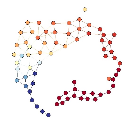
(a) S-Lspline

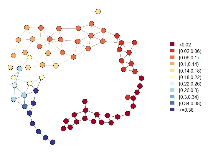
(b) True Value

Figure 12: SDSS Skeleton Colored by values predicted by S-Lspline (left) and by true values (right).

Method	SSE	Parameter
kNN	67.8	neighbor=12
Ridge	870.3	$\lambda=0.001$
Lasso	882.7	$\lambda=0.001$
SpecSeries	66.6	bandwidth = 2
S-Kernel	90.6	bandwidth = $10r_{hns}$
S-kNN	95.8	neighbor = 39
S-Lspline	89.6	-

Table 5: Regression results on SDSS data. The best SSE from each method is listed with the corresponding parameters used.

We perform the same analysis as in Section 4 by comparing the 5-fold cross-validation SSEs of different regression methods on this dataset. Despite the fact that our skeleton-based methods do not show superior performance on this particular dataset, the skeleton representation does reveal the manifold structure in the covariate space and an approximate monotone trend in the response. The clean manifold structure of the data and the small number of covariates may explain the superior performance of kNN and SpecSeries in this case.

6 Conclusion

In this work, we introduce the skeleton regression framework to handle regression problems with manifold-structured inputs. We generalize the nonparametric regression techniques such as kernel smoothing and splines onto graphs. Our methods provide accurate and reliable prediction performance and are capable of recovering the underlying manifold structure of the data. Both theoretical and empirical analyses are provided to illustrate the effectiveness of the skeleton regression procedures.

In what follows, we describe some possible future directions:

• Generalizing skeleton graphs to simplicial complex.
  From a geometric perspective, the skeleton graph constructed in this work only focuses on $0$-simplices (points) and $1$-simplices (line segments). Additional geometric information can be encoded using higher-dimensional simplices. Recent research in deep learning has explored the use of simplicial complices for tasks such as clustering and segmentation (Bronstein et al., 2017; Bodnar et al., 2021). Higher-dimensional simplicies offer a finer approximation to the covariate distribution but have a higher computational cost and a more complex model. Thus, it is unclear if using a higher-dimensional simplex will lead to a better prediction accuracy. We will explore the possibility of extending skeleton graphs to skeleton complex in the future.

• Nonparametric smoothers on graphs.
  The kernel regression and spline regression are not the only possibilities to perform nonparametric smoothing on graphs. For example, Wang et al. (2016) generalized the concept of trend filtering Kim et al. (2009); Tibshirani (2014) to graphs and compared it to Laplacian smoothing and Wavelet smoothing. In contrast to our work, these regression estimators for graphs are applied to data where both the inputs and responses are located on the vertices of a given graph. As a result, these graph smoothers, which include different regularizations, can only fit values on the vertices, and do not model the regression function on the edges (Wang et al. (2016) mentioned the possibility of linear interpolation with the trend filtering).

  It is possible to generalize these methods to skeleton by constructing responses on the knots in the skeleton graph as the mean values of the corresponding Voronoi cell, and then graph smoothers can apply. Some interpolation methods can again be used to predict the responses on the edge, and this can lead to another skeleton-based regression estimator.

• Time-varying covariates and responses.
  A possible avenue for future research is to extend the skeleton regression framework to handle time-varying covariates and responses. Specifically, covariates collected at different time could be used together to construct knots in a skeleton. The edges in the skeleton can change dynamically according to the covariate distribution at different times, providing insight into how the covariate distributions have evolved. Additionally, representing the regression function on the skeleton would make it simple to visualize how the function changes over time.

• Streaming data and online skeleton update. As streaming data becomes increasingly common, a potential area of future research is to investigate methods for updating the skeleton structure and its regression function in a real-time or online fashion. Reconstructing the entire skeleton can be computationally costly, but local updates to edges and knots can be more efficient. We plan to explore ways to develop a simple yet reliable method for updating the skeleton in the future.

Acknowledgments

YC is supported by NSF DMS-195278, 2112907, 2141808 and NIH U24-AG072122. JW is supported by NSF DMS - 2112907.

Appendices

A Skeleton Construction with Voronoi Density

In this section, we provide a more detailed description of the procedures for constructing the skeleton and computing the density-aided edge weight called the Voronoi density, following the work in Wei and Chen (2023).

A.1 Knots Construction

The knots in the skeleton serve as reference points within the data, allowing us to focus our attention from the overall data to these specific locations of interest. We utilize the $k$-means algorithm with a relatively large value of a number of knots $k$ to create these knots in a data-driven way. The number of knots is a crucial parameter in this procedure as it governs the trade-off between the summarizing power of the representation and the preservation of information. Empirical evidence from Wei and Chen (2023) suggests that setting $k$ to around $\sqrt{n}$ can be a helpful reference rule, while the dimensionality of the data should be taken into consideration when choosing $k$.

In practice, since the $k$-means algorithm may not always find the global optimum, we repeat it $1,000$ times with random initial points and select the result corresponding to the optimal objective. We also advise pruning knots with only a small number of with-in-cluster observations. Additionally, it can be helpful to preprocess or denoise the data by removing observations in low-density areas to address issues that could arise for $k$-means clustering.

A.2 Edges Construction

We denote the given knots as $c_{1},\cdots,c_{k}$ and represent their collection as ${\mathcal{C}}={c_{1},\cdots,c_{k}}$. An edge is added between two knots if they are neighbors, which is determined by whether their corresponding Voronoi cells share a common boundary. The Voronoi cell associated with a knot $c_{j}$ is defined as the set of points in ${\mathcal{X}}$ whose distance to $c_{j}$ is the smallest among all knots. That is,

$${\mathbb{C}}_{j}=\{x\in{\mathcal{X}}:d(x,c_{j})\leq d(x,c_{\ell})\ \ \forall\ell\neq j\},$$ (28)

where $d(x,y)$ is the usual Euclidean distance. We add an edge between knots $(c_{i},c_{j})$ if their Voronoi cells have a non-empty intersection. This graph is referred to as the Delaunay triangulation of ${\mathcal{C}}$, denoted as $DT({\mathcal{C}})$.

Although the Delaunay triangulation graph is conceptually intuitive, the computational complexity of the exact Delaunay triangulation algorithm has an exponential dependence on the ambient dimension $d$, making it unfavorable for multivariate or high-dimensional data settings. To overcome this issue, we approximate the Delaunay triangulation with $\hat{DT}({\mathcal{C}})$ by examining the 2-nearest knots of the sample data points. We query the two nearest knots for each data point and add an edge between $c_{i},c_{j}$ if there is at least one data point whose two nearest neighbors are $c_{i},c_{j}$. The computational complexity of this sample-based approximation depends linearly on the dimension $d$, making it suitable for high-dimensional settings.

A.3 Voronoi Density

The Voronoi density (VD) measures the similarity between a pair of knots $(c_{j},c_{\ell})$ based on the number of observations whose 2-nearest knots are $c_{j}$ and $c_{\ell}$. We first define the Voronoi density based on the underlying probability measure and then introduce its sample analog. Given a metric $d$ on ${\mathbb{R}}^{d}$, the 2-Nearest-Neighbor (2-NN) region of a pair of knots $(c_{j},c_{\ell})$ is defined in Equation 1 as

$$B_{j\ell}=\{X_{m},m=1,\dots,n:\left\|x-V_{i}\right\|>\max\{\left\|x-V_{j}\right\|,\left\|x-V_{\ell}\right\|\},\forall i\neq j,\ell\}.$$

Figure 2 provides an illustration of an example 2-NN region of a pair of knots. If two knots $c_{j},c_{\ell}$ are in a connected high-density region, then we expect the 2-NN region of $c_{j},c_{\ell}$ to have a high probability measure. Therefore, the probability ${\mathbb{P}}(B_{j\ell})=P(X_{1}\in B_{j\ell})$ can measure the association between $c_{j}$ and $c_{\ell}$. Based on this insight, the Voronoi density measures the edge weight of $(c_{j},c_{\ell})$ as

$$S_{j\ell}^{VD}=\frac{{\mathbb{P}}(B_{j\ell})}{|c_{j}-c_{\ell}|}.$$ (29)

The Voronoi density adjusts for the fact that 2-NN regions have different sizes by dividing the probability of the in-between region by the mutual Euclidean distance.

In practice, we estimate $S_{j\ell}^{VD}$ by a sample average. The numerator ${\mathbb{P}}(B_{j\ell})$ is estimated by $\hat{P}_{n}(B_{j\ell})=\frac{1}{n}\sum_{i=1}^{n}I(X_{i}\in B_{j\ell})$, and the final estimator for the VD is:

$$\hat{S}_{j\ell}^{VD} =\frac{\hat{P}_{n}({B}_{j\ell})}{|{c}_{j}-{c}_{\ell}|}.$$ (30)

Calculating the Voronoi density is fast. The numerator, which only depends on 2-nearest-neighbors calculation, can be computed efficiently by the k-d tree algorithm. For high-dimensional space, space partitioning search approaches like the k-d tree can be inefficient, but a direct linear search still gives a short run-time.

A.4 Graph Segmentation

After obtaining the weighted skeleton graph, it can be helpful to prune certain edges that are not of interest or segment the skeleton into disconnected components. The edge weights defined above can be utilized to achieve this. We start by first converting the edge weights into dissimilarity measures. Specifically, let ${s_{ij}}{i\neq j}$ be the edge weights, where only connected pairs can take non-zero entries, and let $s{\max}=\max_{i\neq j}s_{ij}$. We then define the corresponding dissimilarities as $d_{ij}=0$ if $i=j$, and $d_{ij}=s_{\max}-s_{ij}$ otherwise. Next, we apply hierarchical clustering using these distances. The choice of linkage criterion for hierarchical clustering depends on the underlying geometric structure of the data. Single linkage is recommended when the components are well-separated, while average linkage works better when there are overlapping clusters of approximately spherical shapes. To determine the resulting segmented skeleton graph, dendrograms can be useful in displaying the clustering structure at different resolutions, and analysts can experiment with different numbers of final clusters and choose a cut that preserves meaningful structures based on the dendrograms. However, it is important to note that the presence of noisy data points may require a larger number of final clusters $S$ to achieve better clustering results.

B Computational Complexity

In this section, we briefly analyze the computational costs of the proposed skeleton regression framework. The first main computational burden of the proposed regression procedure is at the skeleton construction step. Wei and Chen (2023) has provided the computational analysis on this. In particular, when constructing knots, the $k$-means algorithm of Hartigan and Wong (Hartigan and Wong, 1979) has time complexity $O(ndkI)$, where $n$ is the number of points, $d$ is the dimension of the data, $k$ is the number of clusters for $k$-means, and $I$ is the number of iterations needed for convergence. For the edge construction step, the approximate Delaunay Triangulation only depends on the 2-NN neighborhoods, and the k-d tree algorithm for the 2-nearest knot search gives the worst-case complexity of $O(ndk^{(1-1/d)})$. For the edge weights with Voronoi density, the numerator can be computed directly from the $2$-NN search without additional computation and the denominators as pairwise distances between knots can be computed with the worst-case complexity of $O(dk^{2})$.

Given the skeleton, we then project original feature vectors onto the skeleton, which is not much time-consuming. Finding the edge to project onto depends on identifying the two nearest knots, which is provided in the skeleton construction step. Projection is taking inner product computations and takes $O(nd)$ for all the covariates.

The next computational task is to calculate the skeleton-based distance between points on the skeleton. To find the shortest path on a graph between two faraway knots, the general version of Dijkstra’s algorithm (Dijkstra, 1959) takes $\Theta(|{\mathcal{E}}|+|{\mathcal{V}}|^{2})=\Theta(k^{2})$ for each run. However, in practice, we don’t need the $\frac{n(n-1)}{2}$ pairwise distances between all the projected points as the skeleton-based regressors proposed can perform with distances in local neighborhoods, which do not require path-finding algorithm for the skeleton-distance calculation.

With all the pairwise skeleton-based distances between projected feature points given, the S-kernel estimate at one point takes $n_{loc}$ kernel weights computation where $n_{loc}$ refers to the local support of the kernel function. S-Lspline takes $O(n)$ time to transform the data and then a single run of matrix multiplication and inversion to get the coefficients.

C Proofs

C.1 Kernel Regression: Convergence on Edge Point (Theorem 1)

Proof  Let ${\mathcal{B}}(\bm{s},h)\subset{\mathcal{S}}$ be the support for the kernel function $K_{h}(.)$ at point $\bm{s}\in{\mathcal{S}}$ with bandwidth $h$. For an edge point $\bm{s}\in E_{j\ell}\in{\mathcal{E}}$, where ${\mathcal{E}}$ is the overall set of edges defined as open sets. As $n\to\infty,h\to 0$, for sufficiently large $n$, by the property of an open set, we have

$${\mathcal{B}}(\bm{s},h)\subset E_{j\ell}$$

and by our definition of skeleton distance, for two points $\bm{s},\bm{s}^{\prime}\in E_{j\ell}$ on the same edge in the skeleton, $d_{\mathcal{S}}(\bm{s},\bm{s}^{\prime})=\left\|\bm{s}-\bm{s}^{\prime}\right\|$ where $\left\|.\right\|$ denotes the Euclidean distance and is 1-dimensional as parametrized on the same edge. Also we have

$$K_{h}(\bm{s}_{j},\bm{s}_{\ell})\equiv K(d_{\mathcal{S}}(\bm{s}_{j},\bm{s}_{\ell})/h)=K(\left\|\bm{s}_{j}-\bm{s}_{\ell}\right\|/h)=K\left(\frac{\bm{s}_{j}-\bm{s}_{\ell}}{h}\right)$$

Consequently, the skeleton-based kernel regression estimator reduces to

$$\hat{m}_{n}(\bm{s})=\frac{\frac{1}{nh}\sum_{j=1}^{n}Y_{j}K(\frac{\bm{s}_{j}-\bm{s}}{h})}{\frac{1}{nh}\sum_{j=1}^{n}K(\frac{\bm{s}_{j}-\bm{s}}{h})}$$ (31)

and we can use the classical asymptotic results for kernel regression in the continuous case (Bierens, 1983; Wasserman, 2006; Chen, 2017).

Let $\hat{g}_{n}(\bm{s})=\frac{1}{nh}\sum_{j=1}^{n}K\left(\frac{\bm{s}_{j}-\bm{s}}{h}\right)$. We express the difference as

$$\hat{m}_{n}(\bm{s})-m_{\mathcal{S}}(\bm{s}) =\frac{[\hat{m}_{n}(\bm{s})-m_{\mathcal{S}}(\bm{s})]\hat{g}_{n}(\bm{s})}{\hat{g}_{n}(\bm{s})}=\frac{\frac{1}{nh}\sum_{j=1}^{n}[Y_{j}-m_{\mathcal{S}}(\bm{s})]K(\frac{\bm{s}_{j}-\bm{s}}{h})}{\frac{1}{nh}\sum_{j=1}^{n}K(\frac{\bm{s}_{j}-\bm{s}}{h})}$$ (32)

and we analyze the denominator and numerator below.

Let $g(\bm{s})$ be the density at point $\bm{s}$ on the skeleton. For the denominator, we start with the bias:

$$\left|{\mathbb{E}}\hat{g}_{n}(\bm{s})-g(\bm{s})\right| =\left|\frac{1}{h}\int K\bigg{(}\frac{\bm{s}-y}{h}\bigg{)}g(y)dy-g(x)\int K(y)dy\right|$$

$$=\left|\int K(z)[g(\bm{s}-hz)-g(\bm{s})]dz\right|$$

$$\leq\int K(z)C_{1}\left|hz\right|dz=C_{1}h\int K(z)\left|z\right|dz=O(h),$$

where $C_{1}$ is the Lipschitz constant of the density function. For the variance, we have

$${\text{V}ar}\left(\hat{g}_{n}(\bm{s})\right) \leq\frac{1}{nh^{2}}\int K^{2}\bigg{(}\frac{\bm{s}-y}{h}\bigg{)}g(y)dy$$

$$=\frac{1}{nh}\int K^{2}(z)g(\bm{s}-hz)dz$$

$$\leq\frac{1}{nh}\int K^{2}(z)[g(\bm{s})+C_{1}\left|hz\right|]dz$$

$$=\frac{1}{nh}\left[g(\bm{s})\int K^{2}(z)dz+C_{1}h\int K^{2}(z)\left|z\right|dz\right]$$

$$=\frac{1}{nh}g(\bm{s})\int K^{2}(z)dz+o\left(\frac{1}{nh}\right).$$

Putting it altogether, we have

$$\left|\hat{g}_{n}(\bm{s})-g(\bm{s})\right|=O(h)+O_{p}\left(\sqrt{\frac{1}{nh}}\right).$$

Note that we only assume Lipschitz continuity and hence has the bias of rate $O(h)$ rather than the usual $O(h^{2})$ rate with second order smoothness. Higher-order smoothness of $g$ may not improve the overall estimation rate due to the fact that we only have Lipschitz continuity of the regression function.

Now we analyze the numerator of equation (32). We start with the decomposition

$$[\hat{m}_{n}(\bm{s})-m_{\mathcal{S}}(\bm{s})]\hat{g}(\bm{s}) =\underbrace{\frac{1}{nh}\sum_{j=1}^{n}U_{j}K\bigg{(}\frac{\bm{s}-\bm{s}_{j}}{h}\bigg{)}}_{q_{1}(\bm{s})}$$

$$+\underbrace{\frac{1}{n}\sum_{j=1}^{n}\bigg{\{}[m_{\mathcal{S}}(\bm{s}_{j})-m(\bm{s})]K\bigg{(}\frac{\bm{s}-\bm{s}_{j}}{h}\bigg{)}\frac{1}{h}-{\mathbb{E}}\bigg{[}[m_{\mathcal{S}}(\bm{s}_{j})-m_{\mathcal{S}}(\bm{s})]K\bigg{(}\frac{\bm{s}-\bm{s}_{j}}{h}\bigg{)}\frac{1}{h}\bigg{]}\bigg{\}}}_{q_{2}(\bm{s})}$$

$$+\underbrace{\frac{1}{n}\sum_{j=1}^{n}{\mathbb{E}}\bigg{[}[m_{\mathcal{S}}(\bm{s}_{j})-m_{\mathcal{S}}(\bm{s})]K\bigg{(}\frac{\bm{s}-\bm{s}_{j}}{h}\bigg{)}\frac{1}{h}\bigg{]}}_{q_{3}(\bm{s})}.$$

First, we show that

$$q_{1}(\bm{s})=O_{p}\left(\sqrt{\frac{1}{nh}}\right).$$

Let

$$v_{n,j}(\bm{s})=U_{j}K\bigg{(}\frac{\bm{s}-\bm{s}_{j}}{h}\bigg{)}\frac{1}{\sqrt{h}}$$

and we have

$$\sqrt{nh}q_{1}(\bm{s})=\frac{1}{\sqrt{n}}\sum_{j=1}^{n}v_{n,j}(\bm{s}).$$

Thus, its mean is

$${\mathbb{E}}v_{n,j}(\bm{s}) ={\mathbb{E}}\left\{U_{j}K\bigg{(}\frac{\bm{s}-\bm{s}_{j}}{h}\bigg{)}\frac{1}{\sqrt{h}}\right\}=0$$

and the variance is

$${\mathbb{E}}[v_{n,j}(\bm{s})^{2}] ={\mathbb{E}}U_{j}^{2}K\bigg{(}\frac{\bm{s}-\bm{s}_{j}}{h}\bigg{)}^{2}\frac{1}{h}=\int\sigma_{u}^{2}(\bm{s}-hz)g(\bm{s}-hz)K(z)^{2}dz$$

$$\to\sigma_{u}^{2}(\bm{s})g(\bm{s})\int K(z)^{2}dz=O(1),$$

where for the second equality we use the change of variable and by assumption we have $\int K(z)^{2}dz<\infty$. Therefore,

$$q_{1}(\bm{s})=O_{p}\left(\sqrt{\frac{1}{nh}}\right).$$

For the second term, note that ${\mathbb{E}}(q_{2}(\bm{s}))=0$ and the variance is

$${\mathbb{E}}\left[\sqrt{nh}q_{2}(\bm{s})\right]^{2} =\int[m_{\mathcal{S}}(\bm{s}-hz)-m_{\mathcal{S}}(\bm{s})]^{2}g(\bm{s}-hz)K(z)^{2}dz$$

$$\ \ -h\bigg{\{}\int[m_{\mathcal{S}}(\bm{s}-hz)-m_{\mathcal{S}}(\bm{s})]g(\bm{s}-hz)K(z)dz\bigg{\}}^{2}$$

$$\to 0$$

when $h\rightarrow 0$, and hence,

$$q_{2}(\bm{s})=o_{p}\left(\sqrt{\frac{1}{nh}}\right).$$

For the last term, note that we have

$$q_{3}(\bm{s}) =\int[m_{\mathcal{S}}(\bm{s}-hz)-m_{\mathcal{S}}(\bm{s})]g(\bm{s}-hz)K(z)dz$$

$$=\int[m_{\mathcal{S}}(\bm{s}-hz)g(\bm{s}-hz)-m_{\mathcal{S}}(\bm{s})g(\bm{s})]K(z)dz-m_{\mathcal{S}}(\bm{s})\int[g(\bm{s}-hz)-g(\bm{s})]K(z)dz$$

$$\leq C_{1}h\int|z|K(z)dz+C_{2}h\int|z|K(z)dz$$

where $C_{1}$ is the Lipschitz constant for $m(\bm{s})g(\bm{s})$ and $C_{2}$ is the Lipschitz constant for $g(\bm{s})$. Therefore,

$$q_{3}(\bm{s})=O(h)$$

Putting all three terms together, $[\hat{m}(\bm{s})-m(\bm{s})]\hat{g}(\bm{s})=O(h)+O_{p}\left(\sqrt{\frac{1}{nh}}\right)$. As a result, equation (32) becomes

$$\hat{m}_{n}(\bm{s})-m_{\mathcal{S}}(\bm{s}) =\frac{[\hat{m}_{n}(\bm{s})-m_{\mathcal{S}}(\bm{s})]\hat{g}(\bm{s})}{\hat{g}(\bm{s})}=\frac{O(h)+O_{p}\left(\sqrt{\frac{1}{nh}}\right)}{g(\bm{s})+O(h)+O_{p}\left(\sqrt{\frac{1}{nh}}\right)}$$

$$=O(h)+O_{p}\left(\sqrt{\frac{1}{nh}}\right)$$

by Taylor expansion of the fraction.

 

C.2 Kernel Regression: Convergence on Knot with Zero Mass (Proposition 3)

For the ease of proof, we first prove Proposition 3 and then prove Theorem 2.

Proof  Let $\bm{s}\in{\mathcal{V}}$ be a knot with no mass, i.e., $P(\bm{s}_{j}=\bm{s})=0$. The kernel regression can be decomposed as

$$\hat{m}(\bm{s}) =\frac{\frac{1}{n}\sum_{j=1}^{n}Y_{j}K_{h}(\bm{s}_{j},\bm{s})I(\bm{s}_{j}\in{\mathcal{E}}\cap{\mathcal{B}}(\bm{s},h))+\frac{1}{n}\sum_{j=1}^{n}Y_{j}K_{h}(\bm{s}_{j},\bm{s})I(\bm{s}_{j}\in{\mathcal{V}}\cap{\mathcal{B}}(\bm{s},h))}{\frac{1}{n}\sum_{j=1}^{n}K_{h}(\bm{s}_{j},\bm{s})I(\bm{s}_{j}\in{\mathcal{E}}\cap{\mathcal{B}}(\bm{s},h))+\frac{1}{n}\sum_{j=1}^{n}K_{h}(\bm{s}_{j},\bm{s})I(\bm{s}_{j}\in{\mathcal{V}}\cap{\mathcal{B}}(\bm{s},h))}$$

$$=\frac{\frac{1}{n}\sum_{j=1}^{n}Y_{j}K_{h}(\bm{s}_{j},\bm{s})I(\bm{s}_{j}\in{\mathcal{E}}\cap{\mathcal{B}}(\bm{s},h))+\frac{1}{n}\sum_{j=1}^{n}Y_{j}I(\bm{s}_{j}=\bm{s})}{\frac{1}{n}\sum_{j=1}^{n}K_{h}(\bm{s}_{j},\bm{s})I(\bm{s}_{j}\in{\mathcal{E}}\cap{\mathcal{B}}(\bm{s},h))+\frac{1}{n}\sum_{j=1}^{n}I(\bm{s}_{j}=\bm{s})}$$

$$=\frac{\varepsilon_{1,n}(\bm{s})+\nu_{1,n}(\bm{s})}{\varepsilon_{2,n}(\bm{s})+\nu_{2,n}(\bm{s})}.$$

Because $\bm{s}$ is a point without probability mass, $\nu_{1,n}(\bm{s})=\nu_{2,n}(\bm{s})=0$, so the above can further reduce to

$$\hat{m}(\bm{s}) =\frac{\frac{1}{nh}\sum_{j=1}^{n}Y_{j}K_{h}(\bm{s}_{j},\bm{s})I(\bm{s}_{j}\in{\mathcal{E}}\cap{\mathcal{B}}(\bm{s},h))}{\frac{1}{nh}\sum_{j=1}^{n}K_{h}(\bm{s}_{j},\bm{s})I(\bm{s}_{j}\in{\mathcal{E}}\cap{\mathcal{B}}(\bm{s},h))}.$$

However, different from the case on edges, the support of the kernel intersects with multiple edges even when $h\rightarrow 0$, so we study the contribution of each edge individually. Note that when $h\rightarrow 0$, the only knot that exists in the intersection ${\mathcal{B}}(\bm{s},h)\cap{\mathcal{E}}$ is $\bm{s}$. So we only need to consider contributions of edges adjacent to $\bm{s}$.

Let ${\mathcal{I}}$ collect all the edge indices with one knot being $\bm{s}$, i.e., $\ell\in{\mathcal{I}}$ implies that there is an edge between $\bm{s}$ and $\bm{v}_{\ell}\in{\mathcal{V}}$. Let $E_{\ell}$ be the edge connecting $\bm{s}$ and $\bm{v}_{\ell}$. The indicator function $I(\bm{s}_{j}\in{\mathcal{E}}\cap{\mathcal{B}}(\bm{s},h))=\sum_{\ell\in{\mathcal{I}}}I(\bm{s}_{j}\in E_{\ell}\cap{\mathcal{B}}(\bm{s},h)).$ With this, we can rewrite $\hat{m}(\bm{s})$ as

$$\hat{m}(\bm{s}) =\frac{\sum_{\ell\in{\mathcal{I}}}\frac{1}{nh}\sum_{j=1}^{n}Y_{j}K_{h}(\bm{s}_{j},\bm{s})I(\bm{s}_{j}\in E_{\ell}\cap{\mathcal{B}}(\bm{s},h))}{\sum_{\ell\in{\mathcal{I}}}\frac{1}{nh}\sum_{j=1}^{n}K_{h}(\bm{s}_{j},\bm{s})I(\bm{s}_{j}\in E_{\ell}\cap{\mathcal{B}}(\bm{s},h))}$$

$$=\frac{\sum_{\ell\in{\mathcal{I}}}\hat{m}_{n,\ell}(\bm{s})\hat{g}_{n,\ell}(\bm{s})}{\sum_{\ell\in{\mathcal{I}}}\hat{g}_{n,\ell}(\bm{s})}.$$

where

$$\hat{g}_{n,\ell}(\bm{s}) =\frac{1}{nh}\sum_{j=1}^{n}K\left(\frac{\bm{s}_{j}-\bm{s}}{h}\right)I(\bm{s}_{j}\in E_{\ell}\cap{\mathcal{B}}(\bm{s},h)),$$

$$\hat{m}_{n,\ell}(\bm{s})\cdot\hat{g}_{n,\ell}(\bm{s}) =\frac{1}{nh}\sum_{j=1}^{n}Y_{j}K\left(\frac{\bm{s}_{j}-\bm{s}}{h}\right)I(\bm{s}_{j}\in E_{\ell}\cap{\mathcal{B}}(\bm{s},h)).$$

Thus, we will analyze $\hat{g}_{n,\ell}(\bm{s})$ and $\hat{m}_{n,\ell}(\bm{s})\hat{g}_{n,\ell}(\bm{s})$. For a point $\bm{s}_{j}$ on the edge $E_{\ell}$, we can reparamterize it as $\bm{s}_{j}=T_{j}\bm{v}_{\ell}+(1-T_{j})\bm{s}$ for some $T_{j}\in(0,1)$. The location $\bm{s}$ corresponds to the case $T_{j}=0$ and any $\bm{s}_{j}\in E_{\ell}$ will be mapped to $T_{j}>0.$ With this reparameterization, we can write

$$\hat{g}_{n,\ell}(\bm{s}) =\frac{1}{nh}\sum_{j=1}^{n}K\left(\frac{T_{j}}{h}(\bm{v}_{\ell}-\bm{s})\right)I(\bm{s}_{j}\in E_{\ell}\cap{\mathcal{B}}(\bm{s},h)),$$

$$\hat{m}_{n,\ell}(\bm{s})\cdot\hat{g}_{n,\ell}(\bm{s}) =\frac{1}{nh}\sum_{j=1}^{n}Y_{j}K\left(\frac{T_{j}}{h}(\bm{v}_{\ell}-\bm{s})\right)I(\bm{s}_{j}\in E_{\ell}\cap{\mathcal{B}}(\bm{s},h)).$$

To study the limiting behavior when $h\rightarrow 0$, let $g_{\ell}(t)=g((1-t)\bm{s}+t\bm{v}_{\ell})$, $g_{\ell}(0)=\lim_{x\downarrow 0}g_{\ell}(x)$; $m_{\ell}(t)=m_{\mathcal{S}}((1-t)\bm{s}+t\bm{v}_{\ell})$, $m_{\ell}(0)=\lim_{t\downarrow 0}m_{\ell}(t)$; and $\sigma_{\ell}^{2}(t)={\mathbb{E}}(|U_{j}|^{2}|\bm{s}_{j}=(1-t)\bm{s}+t\bm{v}_{\ell})$ , $\sigma_{\ell}^{2}(0)=\lim_{t\downarrow 0}\sigma_{\ell}^{2}(t)$. Then with the new notations, we can write

$${\mathbb{E}}(f(T_{j}(\bm{v}_{\ell}-\bm{s}))I(\bm{s}_{j}\in E_{\ell}\cap{\mathcal{B}}(\bm{s},h))) ={\mathbb{E}}(f(\bm{s}_{j}-s)I(\bm{s}_{j}\in E_{\ell}\cap{\mathcal{B}}(\bm{s},h)))$$

$$=\int_{t>0}f(t)g_{\ell}(t)dt$$

for any integrable function $f$. The bias of the denominator can be written as

$$\left|{\mathbb{E}}\hat{g}_{n,\ell}(\bm{s})-\frac{1}{2}g_{\ell}(0)\right| =\left|\frac{1}{h}\int_{t>0}K\bigg{(}\frac{t}{h}\bigg{)}g_{\ell}(t)dt-g_{\ell}(0)\int_{z>0}K(z)\right|$$

$$=\left|\int_{z>0}K(z)[g_{\ell}(hz)-g_{\ell}(0)]dz\right|$$

$$\leq\int_{z>0}K(z)C_{1}hzdz$$

$$=C_{1}h\int_{z>0}K(z)zdz=O(h).$$

For stochastic variation, we have

$${\text{V}ar}\left(\hat{g}_{n,\ell}(\bm{s})\right) \leq\frac{1}{nh^{2}}\int_{t>0}K^{2}\bigg{(}\frac{t}{h}\bigg{)}g_{\ell}(t)dt$$

$$=\frac{1}{nh}\int_{z>0}K^{2}(z)g(hz)dz$$

$$\leq\frac{1}{nh}\int_{z>0}K^{2}(z)[g(0)+C_{1}\left|hz\right|]dz$$

$$=\frac{1}{nh}\left[g(0)\int_{z>0}K^{2}(z)dz+C_{1}h\int_{z>0}K^{2}(z)\left|z\right|dz\right]$$

$$=O\left(\frac{1}{nh}\right).$$

Thus,

$$\hat{g}_{n}(\bm{s})=\sum_{\ell\in{\mathcal{I}}}\hat{g}_{n,\ell}(\bm{s})=\frac{1}{2}\sum_{\ell\in{\mathcal{I}}}g_{\ell}(0)+O(h)+O_{p}\left(\sqrt{\frac{1}{nh}}\right)$$

For the numerator,

$$\hat{m}_{n,\ell}(\bm{s})\hat{g}_{n,\ell}(\bm{s}) =\underbrace{\frac{1}{nh}\sum_{j=1}^{n}U_{j}K\bigg{(}\frac{t_{j}}{h}\bigg{)}I(\bm{s}_{j}\in E_{\ell}\cap{\mathcal{B}}(\bm{s},h))}_{Q_{1}}$$

$$\qquad+\underbrace{\frac{1}{nh}\sum_{j=1}^{n}m_{\mathcal{S}}(\bm{s}_{j})K\bigg{(}\frac{t_{j}}{h}\bigg{)}I(\bm{s}_{j}\in E_{\ell}\cap{\mathcal{B}}(\bm{s},h))}_{Q_{2}},$$

where $U_{j}=Y_{j}-m_{\mathcal{S}}(\bm{s}_{j})$. Using the fact that ${\mathbb{E}}(U_{j}|\bm{s}_{j})=0$, ${\mathbb{E}}(Q_{1})=0$, and the variance is

$${\text{V}ar}(Q_{1}) \leq\frac{1}{nh^{2}}\int_{t>0}\sigma_{\ell}^{2}(t)K^{2}\bigg{(}\frac{t}{h}\bigg{)}g_{\ell}(t)dt$$

$$=\frac{1}{nh}\int_{z>0}\sigma_{\ell}^{2}(hz)K^{2}(z)g_{\ell}(hz)dz$$

$$=\frac{1}{nh}\int_{z>0}\sigma_{\ell}^{2}(0)K^{2}(z)g_{\ell}(0)dz+O\left(\frac{1}{nh}\right)=O\left(\frac{1}{nh}\right).$$

For $Q_{2}$, we have

$$\left|{\mathbb{E}}(Q_{2})-\frac{m_{\ell}(0)g_{\ell}(0)}{2}\right| =\left|\frac{1}{h}\int_{t>0}m_{\ell}(t)K(t/h)g(t)dt-m_{\ell}(0)g_{\ell}(0)\int_{z>0}K(z)dz\right|$$

$$=\left|\int_{z>0}m_{\ell}(hz)K(z)g_{\ell}(hz)dz-m_{\ell}(0)g_{\ell}(0)\int_{z>0}K(z)dz\right|$$

$$\leq\int_{z>0}\bigg{\{}\big{[}m_{\ell}(0)+C_{2}hz\big{]}\big{[}g_{\ell}(0)+C_{1}hz\big{]}-m_{\ell}(0)g_{\ell}(0)\bigg{\}}K(z)dz$$

$$\leq[C_{1}m_{\ell}(0)+C_{2}g_{\ell}(0)]h\int_{z>0}K(z)zdz+o(h)=O(h).$$

The varaince of $Q_{2}$ is bounded via

$${\text{V}ar}(q_{2}) \leq\frac{1}{nh^{2}}\int_{t>0}m_{\ell}^{2}(t)K^{2}\bigg{(}\frac{t}{h}\bigg{)}g_{\ell}(t)dt$$

$$=\frac{1}{nh}\int_{z>0}m_{\ell}^{2}(hz)K^{2}(z)g_{\ell}(hz)dz$$

$$\leq\frac{1}{nh}\int_{z>0}\left\{m_{\ell}(0)+C_{2}\left|hz\right|\right\}^{2}K^{2}(z)\left\{g_{\ell}(0)+C_{1}\left|hz\right|\right\}dz$$

$$=\frac{1}{nh}\left\{m^{2}_{\ell}(0)g_{\ell}(0)\int_{z>0}zK^{2}(z)dz+O(h)\right\}$$

$$=O\left(\frac{1}{nh}\right)$$

Putting the terms $Q_{1}$ and $Q_{2}$ together, we have

$$\hat{m}_{n,\ell}(\bm{s})\hat{g}_{n,\ell}(\bm{s})=\frac{1}{2}m_{\ell}(0)g_{\ell}(0)+O(h)+O_{p}\left(\sqrt{\frac{1}{nh}}\right).$$

As a result, we conclude that

$$\hat{m}(\bm{s}) =\frac{\sum_{\ell\in{\mathcal{I}}}\hat{m}_{n,\ell}(\bm{s})\hat{g}_{n,\ell}(\bm{s})}{\sum_{\ell\in{\mathcal{I}}}\hat{g}_{n,\ell}(\bm{s})}$$

$$=\frac{\frac{1}{2}\sum_{\ell\in{\mathcal{I}}}m_{\ell}(0)g_{\ell}(0)+O(h)+O_{p}\left(\sqrt{\frac{1}{nh}}\right)}{\frac{1}{2}\sum_{\ell\in{\mathcal{I}}}g_{\ell}(0)+O(h)+O_{p}\left(\sqrt{\frac{1}{nh}}\right)}$$

$$=\frac{\frac{1}{2}\sum_{\ell\in{\mathcal{I}}}m_{\ell}(0)g_{\ell}(0)}{\frac{1}{2}\sum_{\ell\in{\mathcal{I}}}g_{\ell}(0)}+O(h)+O_{p}\left(\sqrt{\frac{1}{nh}}\right)$$

$$=\frac{\sum_{\ell\in{\mathcal{I}}}m_{\ell}(0)g_{\ell}(0)}{\sum_{\ell\in{\mathcal{I}}}g_{\ell}(0)}+O(h)+O_{p}\left(\sqrt{\frac{1}{nh}}\right),$$

which completes the proof.  

C.3 Kernel Regression: Convergence on Knot with Nonzero Mass (Theorem 2)

Proof 

Let $\bm{s}\in{\mathcal{V}}$ be a point where $P(\bm{s}_{j}=\bm{s})=p(\bm{s})>0$. Recall that the kernel regression can be expressed as

$$\hat{m}(\bm{s}) =\frac{\frac{1}{n}\sum_{j=1}^{n}Y_{j}K_{h}(\bm{s}_{j},\bm{s})I(\bm{s}_{j}\in{\mathcal{E}}\cap{\mathcal{B}}(\bm{s},h))+\frac{1}{n}\sum_{j=1}^{n}Y_{j}K_{h}(\bm{s}_{j},\bm{s})I(\bm{s}_{j}\in{\mathcal{V}}\cap{\mathcal{B}}(\bm{s},h))}{\frac{1}{n}\sum_{j=1}^{n}K_{h}(\bm{s}_{j},\bm{s})I(\bm{s}_{j}\in{\mathcal{E}}\cap{\mathcal{B}}(\bm{s},h))+\frac{1}{n}\sum_{j=1}^{n}K_{h}(\bm{s}_{j},\bm{s})I(\bm{s}_{j}\in{\mathcal{V}}\cap{\mathcal{B}}(\bm{s},h))}$$

$$=\frac{\frac{1}{n}\sum_{j=1}^{n}Y_{j}K_{h}(\bm{s}_{j},\bm{s})I(\bm{s}_{j}\in{\mathcal{E}}\cap{\mathcal{B}}(\bm{s},h))+\frac{1}{n}\sum_{j=1}^{n}Y_{j}I(\bm{s}_{j}=\bm{s})}{\frac{1}{n}\sum_{j=1}^{n}K_{h}(\bm{s}_{j},\bm{s})I(\bm{s}_{j}\in{\mathcal{E}}\cap{\mathcal{B}}(\bm{s},h))+\frac{1}{n}\sum_{j=1}^{n}I(\bm{s}_{j}=\bm{s})}$$

$$=\frac{\varepsilon_{1,n}(\bm{s})+\nu_{1,n}(\bm{s})}{\varepsilon_{2,n}(\bm{s})+\nu_{2,n}(\bm{s})}.$$

We look at each term individually and note that we have the edge components terms identical to the proof of Proposition 3, so

$$\varepsilon_{1,n}(\bm{s}) =h\left\{\sum_{\ell\in{\mathcal{I}}}m_{\ell}(0)g_{\ell}(0)+O(h)+O_{p}\left(\sqrt{\frac{1}{nh}}\right)\right\}=O(h)+O_{p}\left(\sqrt{\frac{h}{n}}\right),$$

$$\varepsilon_{2,n}(\bm{s}) =h\left\{\sum_{\ell\in{\mathcal{I}}}g_{\ell}(0)+O(h)+O_{p}\left(\sqrt{\frac{1}{nh}}\right)\right\}=O(h)+O_{p}\left(\sqrt{\frac{h}{n}}\right).$$

For the terms on the knots, they are just a sample average, so

$$\nu_{2,n}(\bm{s})=p(\bm{s})+O_{p}\left(\sqrt{\frac{1}{n}}\right)$$

and similarly

$$\nu_{1,n}(\bm{s}) =\frac{1}{n}\sum_{j=1}^{n}\left(m_{\mathcal{S}}(\bm{s}\right)+U_{j})I(\bm{s}_{j}=\bm{s})$$

$$=m_{\mathcal{S}}(\bm{s})p(\bm{s})+O_{p}\left(\sqrt{\frac{1}{n}}\right).$$

With the fact that $O_{p}\left(\sqrt{\frac{1}{n}}\right)$ dominates $O_{p}\left(\sqrt{\frac{h}{n}}\right)$, we conclude

$$\hat{m}(\bm{s}) =\frac{O(h)+O_{p}\left(\sqrt{\frac{h}{n}}\right)+m_{\mathcal{S}}(\bm{s})p(\bm{s})+O_{p}\left(\sqrt{\frac{1}{n}}\right)}{O(h)+O_{p}\left(\sqrt{\frac{h}{n}}\right)+p(\bm{s})+O_{p}\left(\sqrt{\frac{1}{n}}\right)}$$

$$=\frac{O(h)+O_{p}\left(\sqrt{\frac{1}{n}}\right)}{O(h)+O_{p}\left(\sqrt{\frac{1}{n}}\right)+p(\bm{s})}+\frac{m_{\mathcal{S}}(\bm{s})p(\bm{s})}{O(h)+O_{p}\left(\sqrt{\frac{1}{n}}\right)+p(\bm{s})}$$

$$=\frac{O(h)+O_{p}\left(\sqrt{\frac{1}{n}}\right)}{p(\bm{s})}+O\left[\left(\frac{O(h)+O_{p}\left(\sqrt{\frac{1}{n}}\right)}{p(\bm{s})}\right)^{2}\right]$$

$$\ \ \ \ +m_{\mathcal{S}}(\bm{s})p(\bm{s})\left\{\frac{1}{p(\bm{s})}+\frac{O(h)+O_{p}\left(\sqrt{\frac{1}{n}}\right)}{p(\bm{s})^{2}}\right\}$$

$$=m_{\mathcal{S}}(\bm{s})+O(h)+O_{p}\left(\sqrt{\frac{1}{n}}\right),$$

which completes the proof.

 

D Additional Simulation Results

In this section, we examine the effect of cutting the skeleton into various numbers of disjoint components on the final regression performance. We use the same simulated datasets from Section 4, including Yinyang data, Noisy Yinyang data, and SwissRoll data. The analysis procedure is mainly the same, where we use $5$-fold cross-validation SSE to evaluate the regression results for each dataset and repeat the process 100 times with randomly generated datasets. The main difference is that, during the skeleton construction step, we segment the skeleton graph into different disjoint components using single-linkage hierarchical clustering with respect to the Voronoi Density weights, as outlined in Section 2.1. We then fit and evaluate the skeleton-based regression methods on the skeletons that have been differently cut.

D.1 Vary Skeleton Cuts for Yinyang Data

In this section, we investigate how cutting the skeleton into different numbers of disjoint components affects the performance of skeleton-based methods using the Yinyang data (from Section 4.1). We randomly generate 1000-dimensional Yinyang data 100 times and use $5$-fold cross-validation to calculate the SSE on each dataset. We fit the skeleton-based methods in the same manner as in Section 4, with the exception that the number of knots is fixed at 38 and we cut the initial graph into various numbers of disjoint components (ranging from 1 to 25) when constructing the skeleton. The median 5-fold cross-validation SSEs across the 100 datasets for different numbers of disjoint components are plotted in Figure 13.

Our results show that the S-Lspline method is sensitive to changes in the skeleton structure. In the case of Yinyang data, since there are 5 true disjoint structures in the covariate space, a cut of 5 results in the best regression performance. By design, S-Lspline regressors may incorporate unrelated information from one structure to another when an edge connects two structurally different areas, thus leading to a decline in the regression performance. As a future research, incorporating edge weights into the S-Lspline regressor may help to mitigate the interference between different structures. The S-Kernel regressor also achieves optimal performance when the skeleton is segmented into 5 disjoint components. Skeleton-based kernel regression methods exhibit large changes in performance as the skeleton segmentation changes when the bandwidth is large. This is understandable as larger bandwidth allow more information from large distances, which are more likely to be non-informative as the segmentation changes. On the other hand, S-kNN regressor has best regression performance when the skeleton is left as a fully connected graph. This may be due to the locally adaptive nature of k-nearest-neighbor method that ensure regression result are accurate as long as local neighborhood are identified accurately.

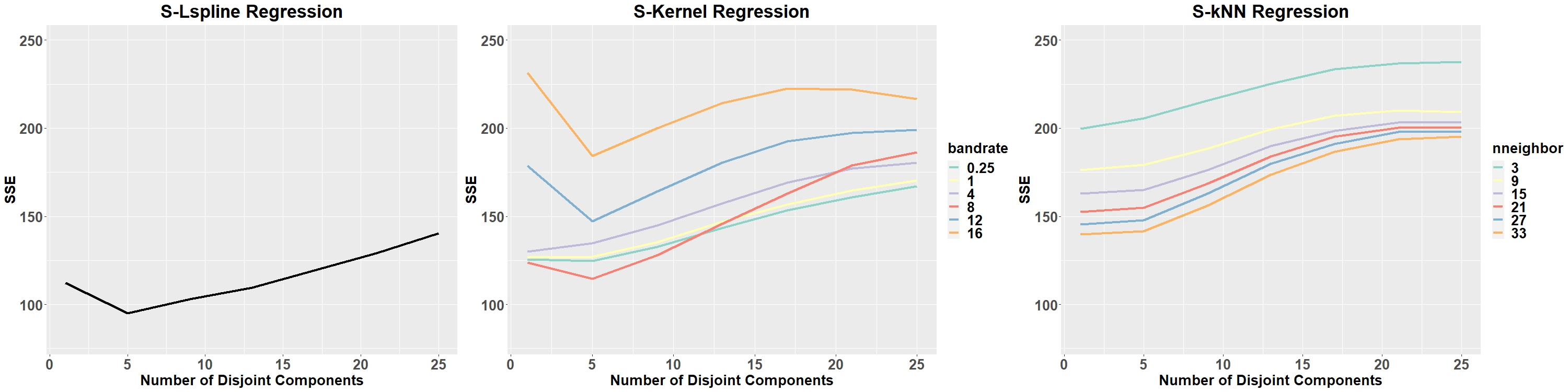
Figure 13: Yinyang $d=1000$ data skeleton regression results with the number of knots fixed as $38$ but segmented into varying numbers of disjoint components. The medium SSE across the $100$ simulated datasets with each given parameter setting is plotted.

D.2 Vary Skeleton Cuts for Noisy Yinyang Data

We then evaluate the performance of the skeleton-based regression methods on the Noisy Yinyang data (from Section 4.2) when the skeletons are constructed with different numbers of disjoint components. Similarly, we randomly generate 1000-dimensional Noisy Yinyang data 100 times and use $5$-fold cross-validation to calculate the sum of squared errors (SSE) on each dataset. We fix the number of knots to be 71 and construct skeletons with different numbers of disjoint components. The median 5-fold cross-validation SSEs across the 100 datasets for different numbers of disjoint components are plotted in Figure 14.

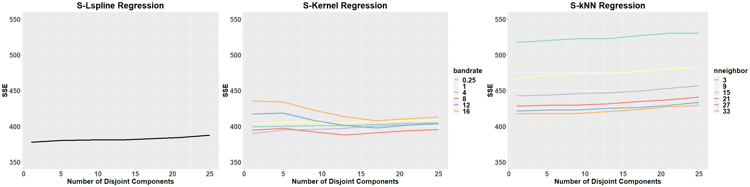
Figure 14: Noise Yinyang $d=1000$ data skeleton regression results with the number of knots fixed as $38$ but segmented into varying numbers of disjoint components. The medium SSE across the $100$ simulated datasets with each given parameter setting is plotted.

With the presence of noise, the S-Lspline method does not show significant variations in performance when the skeleton graph is cut into different disjoint components. The best regression result is obtained when the graph is left as a fully connected graph. In contrast, the performance of the S-kernel method varies with the number of disjoint components. The best results, regardless of the bandwidth, are obtained when the skeleton is segmented into around 13 components, which is larger than the true number of 5 components in the data. Lastly, the S-kNN method demonstrates an increase in SSE with an increase in the number of disjoint components.

D.3 Vary Skeleton Cuts for SwissRoll data

In this section, we evaluate the performance of skeleton-based methods on SwissRoll data (from Section 4.3) with skeletons cut into different numbers of disjoint components. Similarly, we randomly generate 1000-dimensional SwissRoll data 100 times and use $5$-fold cross-validation to calculate the sum of squared errors (SSE) on each dataset. We fix the number of knots to be 70 and construct skeletons with different numbers of disjoint components. The median 5-fold cross-validation SSEs across the 100 datasets for different numbers of disjoint components are plotted in Figure 15.

We find that the S-Lspline regressor is sensitive to changes in the skeleton structure, with the best regression results obtained when the skeleton is constructed as one connected graph. This makes sense as the covariates lie on one connected manifold. The S-Kernel regressor also performs best on the fully-connected skeleton. After an initial increase in SSE as the number of disjoint components increases, the SSE of the S-kernel regressor remains relatively stable. The S-kNN regressor also achieves the best regression performance when the skeleton is left as a fully connected graph. Overall, the SSE of the S-kNN regressor increases with the number of disjoint components, but for a small number of neighbors, there can be a decrease in SSE when the skeleton is cut into more disjoint components. One possible explanation is that, as the response function has discontinuous changes, segmenting the covariate space into more fragments can improve estimation in regions where the response changes abruptly.

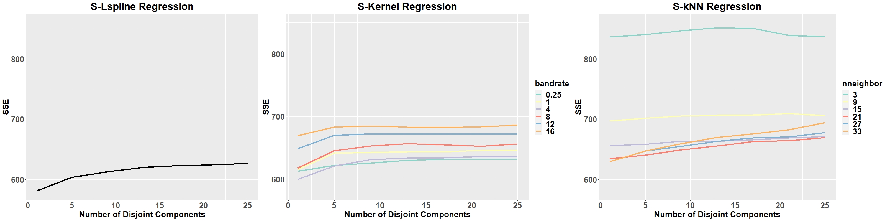
Figure 15: SwissRoll $d=1000$ data skeleton regression results with the number of knots fixed as $70$ but segmented into varying numbers of disjoint components. The medium SSE across the $100$ simulated datasets with each given parameter setting is plotted.

E Additional Real Data Examples

In this section, we present results on some additional examples from the COIL-20 dataset (Nene et al., 1996), following the same procedure as in Section 5.1. Each dataset consists of $72$ gray-scale images of size $128\times 128$ pixels as 2D projections of a 3D object obtained through rotating the object by $72$ equispaced angles on a single axis. The response is the angle of rotation, and to avoid the circular response issue, we remove the last $8$ images from the sequence and only use the first $64$ images from each dataset. We use leave-one-out cross-validation to assess the performance of each method.

E.1 Cup Images Data

We start with a sequence of images of a cup, with some example images in Figure 16. The best SSE from each method is listed in Table 6 along with the corresponding parameters. We see that the S-Lspline method gives the best performance in terms of SSE. The usual kNN regressor also performs well on this data, and it can be due to the different lighting conditions inside the cups that make Euclidean distance between the pixel vectors also reliable for this task.

Figure 16: A part of the cup images from the COIL-20 processed dataset. Each image is of size $128$ pixels.

Method	SSE	Parameter
kNN	1147.2	neighbor=3
Ridge	-	-
Lasso	-	-
SpecSeries	-	-
S-Kernel	2561.5	bandwidth = 4$r_{hns}$
S-kNN	4730.6	neighbor = 3
S-Lspline	1073.4	-

Table 6: Regression results on cup images data from COIL-20. The best SSE from each method is listed with the corresponding parameters used.

E.2 Sauce Box Image Data

We look at another sequence of images taken around a sauce box, with some example images in Figure 17. The best SSE from each method is listed in Table 7 along with the corresponding parameters. In this case, the usual kNN regressor gives the best performance in terms of SSE, while the S-Lspline method gives satisfactory results. The good performance of kNN regressor can be due to the distinctive marks on the box, which makes neighbor search through Euclidean distance on the vectorized image inputs effective. However, the proposed skeleton regression method shows stable performance across different object images and, by explicitly modeling the latent manifold structure, can give a more structured model of the response.

Figure 17: A part of the sauce images from the COIL-20 processed dataset. Each image is of size $128$ pixels.

Method	SSE	Parameter
kNN	955.6	neighbor=3
Ridge	-	-
Lasso	-	-
SpecSeries	-	-
S-Kernel	2998.8	bandwidth = 4$r_{hns}$
S-kNN	5285.4	neighbor = 6
S-Lspline	1220.1	-

Table 7: Regression results on sauce images data from COIL-20. The best SSE from each method is listed with the corresponding parameters used.

References

- Alam et al. (2015) S. Alam, F. D. Albareti, C. A. Prieto, F. Anders, S. F. Anderson, T. Anderton, B. H. Andrews, E. Armengaud, É. Aubourg, S. Bailey, et al. The eleventh and twelfth data releases of the sloan digital sky survey: final data from sdss-iii. The Astrophysical Journal Supplement Series, 219(1):12, 2015.
- Altman (1992) N. S. Altman. An introduction to kernel and nearest-neighbor nonparametric regression. American Statistician, 46:175–185, 1992. ISSN 15372731. doi: 10.1080/00031305.1992.10475879.
- Aswani et al. (2011) A. Aswani, P. Bickel, and C. Tomlin. Regression on manifolds: Estimation of the exterior derivative. The Annals of Statistics, 39(1):48 – 81, 2011. doi: 10.1214/10-AOS823. URL https://doi.org/10.1214/10-AOS823.
- Babenko and Lempitsky (2012) A. Babenko and V. Lempitsky. The inverted multi-index. In 2012 IEEE Conference on Computer Vision and Pattern Recognition, pages 3069–3076, 2012. doi: 10.1109/CVPR.2012.6248038.
- Belkin et al. (2006) M. Belkin, P. Niyogi, and V. Sindhwani. Manifold regularization: A geometric framework for learning from labeled and unlabeled examples. Journal of Machine Learning Research, 7(85):2399–2434, 2006. URL http://jmlr.org/papers/v7/belkin06a.html.
- Bierens (1983) H. J. Bierens. Uniform consistency of kernel estimators of a regression function under generalized conditions. Journal of the American Statistical Association, 78(383):699–707, 1983. ISSN 01621459. URL http://www.jstor.org/stable/2288140.
- Bodnar et al. (2021) C. Bodnar, F. Frasca, Y. Wang, N. Otter, G. F. Montufar, P. Lió, and M. Bronstein. Weisfeiler and lehman go topological: Message passing simplicial networks. In M. Meila and T. Zhang, editors, Proceedings of the 38th International Conference on Machine Learning, volume 139 of Proceedings of Machine Learning Research, pages 1026–1037. PMLR, 18–24 Jul 2021. URL https://proceedings.mlr.press/v139/bodnar21a.html.
- Breiman (2017) L. Breiman. Classification and regression trees. Routledge, 2017.
- Bronstein et al. (2017) M. M. Bronstein, J. Bruna, Y. LeCun, A. Szlam, and P. Vandergheynst. Geometric deep learning: Going beyond euclidean data. IEEE Signal Processing Magazine, 34(4):18–42, 2017. doi: 10.1109/MSP.2017.2693418.
- Chen (2017) Y.-C. Chen. A tutorial on kernel density estimation and recent advances, 2017.
- Cheng and Wu (2013) M.-Y. Cheng and H.-T. Wu. Local linear regression on manifolds and its geometric interpretation. Journal of the American Statistical Association, 108(504):1421–1434, 2013. doi: 10.1080/01621459.2013.827984.
- Dijkstra (1959) E. W. Dijkstra. A note on two problems in connexion with graphs. NUMERISCHE MATHEMATIK, 1(1):269–271, 1959.
- Fan and Fan (1992) J. Fan and J. Fan. Design-adaptive Nonparametric Regression. Journal of the American Statistical Association, 87(420):998–1004, 1992.
- Fan and Gijbels (2018) J. Fan and I. Gijbels. Local polynomial modelling and its applications. Routledge, 2018.
- Fan et al. (1996) J. Fan, I. Gijbels, T. C. Hu, and L. S. Huang. A study of variable bandwidth selection for local polynomial regression. Statistica Sinica, 6(1):113–127, 1996. ISSN 10170405.
- Friedman (1991) J. H. Friedman. Multivariate adaptive regression splines. https://doi.org/10.1214/aos/1176347963, 19:1–67, 3 1991. ISSN 0090-5364. doi: 10.1214/AOS/1176347963.
- Green et al. (2021) A. Green, S. Balakrishnan, and R. Tibshirani. Minimax optimal regression over sobolev spaces via laplacian regularization on neighborhood graphs. In A. Banerjee and K. Fukumizu, editors, Proceedings of The 24th International Conference on Artificial Intelligence and Statistics, volume 130 of Proceedings of Machine Learning Research, pages 2602–2610. PMLR, 13–15 Apr 2021.
- Guhaniyogi and Dunson (2016) R. Guhaniyogi and D. B. Dunson. Compressed gaussian process for manifold regression. Journal of Machine Learning Research, 17(69):1–26, 2016. URL http://jmlr.org/papers/v17/14-230.html.
- Györfi et al. (2002) L. Györfi, M. Kohler, A. Krzyżak, and H. Walk. A Distribution-Free Theory of Nonparametric Regression. Springer New York, 2002. ISBN 978-0-387-95441-7. doi: 10.1007/B97848. URL http://link.springer.com/10.1007/b97848.
- Hartigan and Wong (1979) J. A. Hartigan and M. A. Wong. Algorithm AS 136: A K-Means Clustering Algorithm. Applied Statistics, 28(1):100, 1979. ISSN 00359254. doi: 10.2307/2346830.
- Hastie and Loader (1993) T. Hastie and C. Loader. [local regression: Automatic kernel carpentry]: Rejoinder. https://doi.org/10.1214/ss/1177011005, 8:139–143, 5 1993. ISSN 0883-4237. doi: 10.1214/SS/1177011005.
- Hastie et al. (2009) T. Hastie, R. Tibshirani, and J. Friedman. The Elements of Statistical Learning. Springer New York, 2009. ISBN 978-0-387-84857-0. doi: 10.1007/978-0-387-84858-7. URL http://link.springer.com/10.1007/978-0-387-84858-7.
- Kim et al. (2009) S. J. Kim, K. Koh, S. Boyd, and D. Gorinevsky. trend filtering. http://dx.doi.org/10.1137/070690274, 51:339–360, 5 2009. ISSN 00361445. doi: 10.1137/070690274.
- Kpotufe (2009) S. Kpotufe. Fast, smooth and adaptive regression in metric spaces. Advances in Neural Information Processing Systems, 22, 2009.
- Kpotufe (2011) S. Kpotufe. k-nn regression adapts to local intrinsic dimension. Advances in Neural Information Processing Systems 24: 25th Annual Conference on Neural Information Processing Systems 2011, NIPS 2011, 10 2011. URL https://arxiv.org/abs/1110.4300v1.
- Kpotufe and Garg (2013) S. Kpotufe and V. K. Garg. Adaptivity to local smoothness and dimension in kernel regression. Advances in Neural Information Processing Systems, 26, 2013.
- Kpotufe and Verma (2017) S. Kpotufe and N. Verma. Time-accuracy tradeoffs in kernel prediction: Controlling prediction quality. Journal of Machine Learning Research, 18(44):1–29, 2017. URL http://jmlr.org/papers/v18/16-538.html.
- Lee and Izbicki (2016) A. B. Lee and R. Izbicki. A spectral series approach to high-dimensional nonparametric regression. Electronic Journal of Statistics, 10(1):423 – 463, 2016. doi: 10.1214/16-EJS1112. URL https://doi.org/10.1214/16-EJS1112.
- Lin and Yao (2020) Z. Lin and F. Yao. Functional regression on the manifold with contamination. Biometrika, 108(1):167–181, 07 2020. ISSN 0006-3444. doi: 10.1093/biomet/asaa041. URL https://doi.org/10.1093/biomet/asaa041.
- Loh (2014) W.-Y. Loh. Fifty years of classification and regression trees. International Statistical Review, 82(3):329–348, 2014.
- Marzio et al. (2014) M. D. Marzio, A. Panzera, and C. C. Taylor. Nonparametric regression for spherical data. Journal of the American Statistical Association, 109(506):748–763, 2014. doi: 10.1080/01621459.2013.866567. URL https://doi.org/10.1080/01621459.2013.866567.
- Massy (1965) W. F. Massy. Principal components regression in exploratory statistical research. Journal of the American Statistical Association, 60(309):234–256, 1965. doi: 10.1080/01621459.1965.10480787. URL https://www.tandfonline.com/doi/abs/10.1080/01621459.1965.10480787.
- Morrison et al. (2017) C. B. Morrison, H. Hildebrandt, S. J. Schmidt, I. K. Baldry, M. Bilicki, A. Choi, T. Erben, and P. Schneider. The-wizz: Clustering redshift estimation for everyone. Monthly Notices of the Royal Astronomical Society, 467(3):3576–3589, 2017.
- Nadaraya (1964) E. A. Nadaraya. On estimating regression. http://dx.doi.org/10.1137/1109020, 9:141–142, 7 1964. ISSN 0040-585X. doi: 10.1137/1109020.
- Nene et al. (1996) S. A. Nene, S. K. Nayar, and H. Murase. Columbia object image library (coil-20). Technical report, Columbia University, 2 1996. URL https://www.cs.columbia.edu/CAVE/software/softlib/coil-20.php.
- Rahman et al. (2015) M. Rahman, B. Ménard, R. Scranton, S. J. Schmidt, and C. B. Morrison. Clustering-based redshift estimation: comparison to spectroscopic redshifts. Monthly Notices of the Royal Astronomical Society, 447(4):3500–3511, 2015.
- Schölkopf and Smola (2002) B. Schölkopf and A. J. Smola. Learning with Kernels: Support Vector Machines, Regularization, Optimization, and Beyond Adaptive computation and machine learning. The MIT Press, 2002. ISBN 9780262194754.
- Sivic and Zisserman (2003) Sivic and Zisserman. Video google: a text retrieval approach to object matching in videos. In Proceedings Ninth IEEE International Conference on Computer Vision, pages 1470–1477 vol.2, 2003. doi: 10.1109/ICCV.2003.1238663.
- Tibshirani (2014) R. J. Tibshirani. Adaptive piecewise polynomial estimation via trend filtering. The Annals of Statistics, 42(1):285–323, 2014. ISSN 00905364. URL http://www.jstor.org/stable/43556281.
- Torrence and Compo (1998) C. Torrence and G. P. Compo. A practical guide to wavelet analysis. Bulletin of the American Meteorological society, 79(1):61–78, 1998.
- Wahba (1975) G. Wahba. Smoothing noisy data with spline functions. Numerische mathematik, 24(5):383–393, 1975.
- Walesiak and Dudek (2020) M. Walesiak and A. Dudek. The choice of variable normalization method in cluster analysis. In K. S. Soliman, editor, Education Excellence and Innovation Management: A 2025 Vision to Sustain Economic Development During Global Challenges, pages 325–340. International Business Information Management Association (IBIMA), 2020. ISBN 978-0-9998551-4-1.
- Wang (2011) Y. Wang. Smoothing splines: methods and applications. CRC press, 2011.
- Wang et al. (2016) Y. X. Wang, J. Sharpnack, A. J. Smola, and R. J. Tibshirani. Trend filtering on graphs. Journal of Machine Learning Research, 17:1–41, 2016. ISSN 15337928.
- Wasserman (2006) L. Wasserman. All of nonparametric statistics. Springer Science & Business Media, 2006.
- Watson (1964) G. S. Watson. Smooth regression analysis. Sankhyā: The Indian Journal of Statistics, Series A (1961-2002), 26(4):359–372, 1964. ISSN 0581572X. URL http://www.jstor.org/stable/25049340.
- Wei and Chen (2023) Z. Wei and Y.-C. Chen. Skeleton clustering: Dimension-free density-aided clustering. Journal of the American Statistical Association, 0(ja):1–30, 2023. doi: 10.1080/01621459.2023.2174122.
- Wold (1975) H. Wold. Soft modelling by latent variables: The non-linear iterative partial least squares (nipals) approach. Journal of Applied Probability, 12:117–142, 1975. ISSN 0021-9002. doi: 10.1017/S0021900200047604.
- York et al. (2000) D. G. York, J. Adelman, J. E. Anderson Jr, S. F. Anderson, J. Annis, N. A. Bahcall, J. Bakken, R. Barkhouser, S. Bastian, E. Berman, et al. The sloan digital sky survey: Technical summary. The Astronomical Journal, 120(3):1579, 2000.
- Zhang et al. (2019) X. Zhang, X. Shi, Y. Sun, and L. Cheng. Multivariate regression with gross errors on manifold-valued data. IEEE Transactions on Pattern Analysis and Machine Intelligence, 41(2):444–458, 2019. doi: 10.1109/TPAMI.2017.2776260.
- Zhang et al. (2013) Y. Zhang, J. Duchi, and M. Wainwright. Divide and conquer kernel ridge regression. In S. Shalev-Shwartz and I. Steinwart, editors, Proceedings of the 26th Annual Conference on Learning Theory, volume 30 of Proceedings of Machine Learning Research, pages 592–617, Princeton, NJ, USA, 12–14 Jun 2013. PMLR. URL https://proceedings.mlr.press/v30/Zhang13.html.