QuantumDynamics.jl: A modular approach to simulations of dynamics of open quantum systems

Abstract

Simulation of non-adiabatic dynamics of a quantum system coupled to dissipative environments poses significant challenges. New sophisticated methods are regularly being developed with an eye towards moving to larger systems and more complicated description of solvents. Many of these methods, however, are quite difficult to implement and debug. Furthermore, trying to make the individual algorithms work together through a modular application programming interface (API) can be quite difficult. We present a new, open-source software framework, QuantumDynamics.jl, designed to address these challenges. It provides implementations of a variety of perturbative and non-perturbative methods for simulating the dynamics of these sytems. Most prominently, QuantumDynamics.jl supports hierarchical equations of motion and the family of methods based on path integrals. Effort has been made to ensure maximum compatibility of interface between the various methods. Additionally, QuantumDynamics.jl, being built on a high-level programming language, brings a host of modern features to explorations of systems such as usage of Jupyter notebooks and high level plotting, possibility of leveraging high-performance machine learning libraries for further development. Thus, while the built-in methods can be used as end-points in themselves, the package provides an integrated platform for experimentation, exploration, and method development.

I Introduction

Understanding the evolution of a system over time is at the heart of chemistry and physics. While many systems can indeed be treated classically, there are several important problems where the quantum mechanical mechanism of tunneling becomes inescapable. Some of the most ubiquitous of these are charge transfer problems, excitation energy transfer processes and spin dynamics. Additionally, in all these cases the dynamics may be severely modulated by the existence of solvent degrees of freedom which exist at a given temperature. The necessity of simulating the systems quantum mechanically while accounting for the environment and solvents accurately prove to be significantly challenging.

Various approaches exist to tackle this problem. On the end of approximate approaches there is the perturbative Bloch-Redfield Master Equations [1, 2] (BRME) and methods based on empirical Lindbladians. However, these are uncontrolled approximations with no good error bounds. Therefore it becomes important to be able to obtain the exact dynamics for these systems. Various path integral-based techniques like the quasi-adiabatic propagator path integral [3, 4, 5] (QuAPI) family of methods and hierarchy equations of motion [6, 7, 8] (HEOM) family of methods exist which at greater costs can simulate the full non-Markovian dynamics of a quantum system coupled with dissipative media using the Feynman-Vernon influence functional [9]. Over the years, methods of unparallelled sophistication have been built on both these frameworks which reduce the computational costs of simulations [10, 11, 12, 13, 14, 15, 16, 17, 18, 19, 20, 21, 22, 23, 24, 25, 26].

Despite the existence of a multitude of rigorous methods, software support for quantum dynamics is relatively sparse. The situation becomes especially stark when put in comparison to the plethora of alternatives, both open-source and proprietary, that exist for electronic structure theory [27, 28, 29, 30, 31, 32, 33, 34]. The lack of easily available implementation of the latest methods prevent their widespread adoption. In addition to preventing people from both being able to apply these novel ideas to a variety of problems, this has the inadvertent disadvantage of preventing critical comparison and evaluation of the different methods. In terms of providing access to multiple state-of-the-art algorithms for dynamics in a single package, i-PI [35] is exemplary, providing flexible implementations of various methods based on imaginary time path integral and approximate quantum dynamics using ring-polymer. However, it does not support approaches for simulating non-adiabatic processes.

Amongst exact methods for simulating processes that can be decomposed in terms of a quantum system interacting with a thermal bath, HEOM has a fair number of implementations [36, 37, 38, 39]. QuTiP [40], which supports a plethora of approximate methods for simulating open quantum systems, has an implementation of HEOM. A C++/Python software called Libra [41] and a new Julia package called NQCDynamics.jl [42] have been developed primarily for using classical trajectory-based methods for simulating non-adiabatic quantum dynamics. However, when it comes to numerically “exact” simulation of these systems and supporting the variety of state-of-the-art real time path integral-based methods in a modular fashion, there is a severe dearth of software. This has been a significant impediment in the approachability, adoption and further development of these powerful methods.

Most computational codes have been historically written in C or C++ or Fortran. While performant, these languages are low-level and their use significantly adds to the code complexity and raises the bar for others contributing to the frameworks. Of late, Python is being used for writing scientific code, with the most performance intensive parts written in C or C++. Prime examples of programs and packages using this “two-language” infrastructure are PySCF [30], Psi4 [29], i-PI [35], etc. A relatively new language called Julia [43], with promise in terms of balancing performance with ease of use, has been gaining popularity in the scientific community. It features a just-in-time compilation scheme that solves the two-language problem, where the API exposes features to a high-level language but the performance-critical parts are coded in a different low-level language. It consequently becomes easy to have scientific packages written completely in Julia without sacrificing performance. There has been an explosion of packages for computational chemistry in Julia in the recent past [44, 42, 45, 46, 47, 48].

We introduce a new open-source software package for the Julia language called QuantumDynamics.jl for providing easy access to the state-of-the-art tools for rigorous simulation of non-adiabatic systems to the community. An implementation in a high-performance, high-level language is convenient for widespread adoption and easy development in the future. Though it supports some approximate methods, the primary focus of QuantumDynamics.jl is methods for numerically exact simulations of non-adiabatic problems. The design aims at providing atomic concepts that help maximize reuse of code between a diverse set of path integral-based methods. The paper is organized as follows. Online documentation has already been provided. It will continue to be maintained, updated, and improved upon as the package changes. In Sec. II, we discuss the methods supported in QuantumDynamics.jl and the structure of the package. We demonstrate the usage of the package through representative examples of the methods. While code snippets have been provided in this paper, the full examples are there in the examples folder of the repository. Some concluding remarks are provided in Sec. IV.

II Methods Supported and Structure of the Code

II.1 Methods Supported

The main focus of QuantumDynamics.jl is the simulation of dynamics of open quantum systems with non-adiabatic processes. These are characterized a relatively small dimensional quantum system, described by a Hamiltonian, $\hat{H}_{0}$, interacting with $N_{\text{env}}$ large thermal environments.

$$\hat{H} =\hat{H}_{0}+\sum_{b}^{N_{\text{env}}}\hat{H}^{(b)}_{\text{env}}$$ (1)

$$\hat{H}^{(b)}_{\text{env}} =\sum_{j}\frac{p_{jb}^{2}}{2m_{jb}}+\frac{1}{2}m_{jb}\omega_{jb}^{2}\left(x_{jb}-\frac{c_{jb}\hat{s}_{b}}{m_{jb}\omega_{jb}^{2}}\right)^{2},$$ (2)

where $\omega_{jb}$ and $c_{jb}$ are the frequency and coupling of the $j$th mode of the $b$th environment. The interaction between the system and the $b$th environment is described by $\hat{H}^{(b)}_{\text{env}}$ and happens through the system operator $\hat{s}_{b}$. In general the environments are atomistically defined. However, under Gaussian response limit, it is possible to map the effects of the atomistic environment onto a bath of harmonic oscillators [49, 50, 51, 52] through the energy gap auto-correlation function and its spectral density,

$$J_{b}(\omega) =\frac{\pi}{2}\sum_{j}\frac{c_{jb}^{2}}{m_{jb}\omega_{jb}}\delta(\omega-\omega_{jb}).$$ (3)

The famous spin-boson model is a specialization of Eq. 1 for the case of $\hat{H}_{0}=\epsilon\sigma_{z}-\hbar\Omega\sigma_{x}$, where $\epsilon$ is the asymmetry between the two states and $\Omega$ is the coupling strength. Spin-boson models typically have a single harmonic bath as an environment. Two of the most common model spectral densities are

$$J_{\text{ExpCutoff}}(\omega,n) =\frac{2\pi}{\Delta s^{2}}\hbar\xi\frac{\omega^{n}}{\omega_{c}^{n-1}}\exp\left(-\frac{\omega}{\omega_{c}}\right),$$ (4)

$$\text{and }J_{\text{DrudeLorentz}}(\omega) =\frac{2\lambda}{\Delta s^{2}}\frac{\gamma\omega}{\omega^{2}+\gamma^{2}}.$$ (5)

Here $\Delta s$ is the separation between the system states. Depending on the value of $n$, $J_{\text{ExpCutoff}}$ represents an Ohmic spectral density ($n=1$), super-Ohmic spectral density ($n>1$) or sub-Ohmic spectral density ($n<1$). This family of spectral densities is specified in terms of the dimensionless Kondo parameter, $\xi$, and the cutoff frequency, $\omega_{c}$. The Drude-Lorentz spectral density is another Ohmic spectral density but with a Lorentzian cutoff. It is typically specified using a reorganization energy, $\lambda$, and the characteristic bath time scale, $\gamma$.

There are a variety of approaches for simulating the dynamics of these systems ranging from completely empirical to numerically exact. The implementations are often challenging and hard to bring to a common interface. Because of the typically strong system-environment couplings, perturbative methods of calculation of dynamics are often not very accurate. However, they still might provide useful starting points for understanding the dynamics. A broad set of these exact and approximate methods are supported in QuantumDynamics.jl. They can be roughly categorized as

1. Empirical approaches

2. Hierarchical Equations of Motion

3. Path integral approaches

It is often difficult to maintain consistency of the interface across these different classes of approaches. However, within every category, the consistency has been ensured. QuantumDynamics.jl does not support the rich gamut of classical trajectory-based methods. Consequently, notable in its omission is the ubiquitous surface hopping method [53, 54, 55]. The NQCDynamics.jl package [42] implements surface hopping both in its fewest switching form and in connection to ring-polymer molecular dynamics. It also implements various other classical trajectory-based approaches in a modular manner.

Within the group of empirical approaches, QuantumDynamics.jl supports propagation of both Hermitian and non-Hermitian systems. It also supports more rigorous approaches based on master equations such as BRME and Lindblad master equation. HEOM [6, 7, 56, 57] is implemented in its “scaled” form [23]. While many other improvements and extensions of HEOM exist in the literature, they have not yet been implemented in QuantumDynamics.jl. These will be incorporated in future versions as and when required.

The largest class of methods supported by QuantumDynamics.jl is in the path integral approaches. In addition to the original QuAPI [3, 4, 5], blip decomposition of path integrals [10, 11] (BSPI), the tensor network path integral [15] implementation of time-evolving matrix product operator [21] (TEMPO) approach and the pairwise-connected tensor network path integral [12] (PC-TNPI) method are supported. Quantum-classical path integral [58, 59] (QCPI) using solvent-driven references [60] in the harmonic backreaction [61] framework has been implemented using the same interface. As elaborated in Sec. II.2, the code has been designed in a way that QCPI could be used with different “backends” corresponding to QuAPI or TEMPO.

Ideas of dynamical maps have been shown to be effective in understanding non-Markovian evolution of systems [62]. The transfer tensor method [62] (TTM) allows construction of transfer tensors from dynamical maps, which for open quantum systems are the forward-backward propagators augmented by the bath influence, $\mathcal{E}(t)=\Tr_{\text{bath}}\left(\exp\left(-i\mathcal{L}t/\hbar\right)\right)$, where $\mathcal{L}$ is the Liouvillean corresponding to the system-bath. These transfer tensors can be further used to propagate the reduced density matrix of the system beyond the memory length. This reduces the complexity of simulating the time-evolution beyond memory length to multiplying matrices of the size of the system and removes all storage requirements. TTM in QuantumDynamics.jl can take advantage of the forward-backward augmented propagators obtained from other path integral methods like QuAPI, TEMPO, PC-TNPI, and blips.

The small matrix decomposition of path integral [17, 18] (SMatPI) is a rigorous QuAPI-based method which achieves a similar objective but with more efficient implementations for extended memory length [20] and support for simulation of dynamics under the influence of external fields [63]. It has been noted by Makri [18] that while TTM employs time-translational invariance leading to generation of spurious memory, SMatPI through a rigorous derivation based on QuAPI lifts this limitation. QuantumDynamics.jl enables the use of tensor network-based methods like TEMPO with TTM which allows inclusion of the possible spurious memory generated without a significant increase in computational complexity.

All these methods with the exception of TTM have been implemented in a manner so that they can simulate the dynamics of these systems in presence of external time-dependent fields. One of the potential applications of such time-dependent fields is simulation of dynamics in the presence of light described in a semiclassical manner.

II.2 Code Structure

QuantumDynamics.jl, being a Julia package, can be used on any operating system and platform supported by the programming language. It has recently been registered with the Julia package registry. Thus, the installation procedure is relatively simple. After Julia has been setup, there are two ways of installing QuantumDynamics.jl. The first way involves Julia’s package manager read-eval-print loop (REPL) interface:

⬇

julia> ]

pkg> add QuantumDynamics

The alternate is to use the Pkg module in Julia:

⬇

import Pkg

Pkg.add(”QuantumDynamics”)

All the dependencies will automatically be installed. Julia comes with implementations of OpenBlas built-in by default. However, depending on the architecture, it may be preferable to install and use Intel’s Math Kernel Library (MKL), which can be installed as an additional package MKL.jl. If MKL is used, it should be loaded before QuantumDynamics.jl in the source code.

In QuantumDynamics.jl, an attempt has been made to provide as flexible and consistent an application programming interface (API) as possible across the gamut of supported methods. This consistency is crucial in ensuring a successful mix-and-match of various approaches. However, this is an extremely challenging task given the different requirements and restrictions of various methods. In this section, we discuss some of the crucial design choices present in this package.

Each method has its own module. The empirical methods are completely grouped in the Bare module. Bloch-Redfield Master Equation [2, 1] and HEOM [57] are supported in the BlochRedfield and HEOM modules respectively. The path integral methods are more varied and have been afforded their individual modules viz. QuAPI [3, 4], Blip [10], TEMPO [21], PCTNPI [12], etc. All the path integral methods, with the exception of quantum-classical path integral [58, 59], builds on top of a time-series of forward-backward propagators corresponding to the bare or isolated system. Because of this decision, it becomes possible for QCPI to use any of the base path integral methods as the engine to simulate the dynamics. For every sampled phase space point of the solvent, the QCPI routine provides the underlying path integral routine a sequence of solvent-driven reference propagators [60], and obtains as an output the reduced density matrices after incorporation of the backreaction in the harmonic approximation [61]. The toggle of whether the full memory needs to be incorporated or just the quantum memory from the back reaction is necessary, is determined by the boolean parameter, reference_propagator. If reference_propagator is false, which is the default behavior, then the full influence functional is incorporated, else only the quantum memory is incorporated. For any method, the function for simulating the dynamics of an reduced density matrix is called propagate. Individual methods often have convergence parameters that differ wildly from each other. All such parameters are grouped in method-specific argument types all derived from Utilities.ExtraArgs.

QCPI requires definition of a solvent, which is treated by classical trajectories. This facility is provided by the abstract struct Solvents.Solvent, which can be inheritted from for different types of solvents. Currently only a discrete harmonic bath is provided. There is scope for providing wrappers around emerging Julia libraries for doing molecular dynamics as more detailed solvents. Associated with each solvent is a description of the corresponding phase space, and an iterator which generates phase space points that are distributed according to the thermal Boltzmann distribution.

Many of the empirical methods and HEOM require solution of differential equations, which is done numerically using the DifferentialEquations.jl [64] package. It implements a variety of methods for solving differential equations. The details that control differential equation solver like the method of simulation, relative error and absolute error, are controlled through the structure, Utilities.DiffEqArgs. In QuantumDynamics.jl, the default method of solution is an adaptive Runge-Kutta approach of orders 5 (4) [65], though other methods can be easily used by suitably changing the Utilities.DiffEqArgs passed to the method. The methods based on tensor network are built on the open-source ITensor [66, 67] library.

For the specification of the bath spectral densities, QuantumDynamics.jl provides a SpectralDensities module. Currently we support ExponentialCutoff for Eq. 4 and DrudeLorentz for Eq. 5. Facilities are provided for reading in tabulated spectral densities obtained as Fourier transforms of numerically simulated bath response functions is also provided through SpectralDensityTable. Utility functions are provided for reading the tabulated data for both $J(\omega)$ and $J(\omega)/\omega$.

Finally, TTM [62] builds on propagators from initial time, $t=0$, to final time. Thus, in addition to providing routines for propagating a reduced density matrix, the various sub-modules for path integral also provide build_augmented_propagator functions that calculate the time-series of propagators including the solvent effects using the corresponding full path methods. As detailed in the numerical examples, Sec. III, these functions make it possible to use TTM to propagate a system whose augmented propagators have been calculated using some path integral method.

The full documentation of the package also shows other examples along with detailed description of the various arguments and parameters supported by these methods. It will remain updated as the package continues to evolve and implement other methods.

III Numerical Examples

III.1 Empirical Approaches to Open Quantum Systems

III.1.1 Isolated Hermitian & Non-Hermitian Systems

The simplest case of propagation happens to be for an isolated system. The dynamics is Markovian. QuantumDynamics.jl provides interface for simulating this dynamics both for Hermitian and non-Hermitian systems defined by a Hamiltonian, $\hat{H}$. The equation of motion for the density matrix,

$$i\hbar\partial_{t}\rho(t)=\hat{H}\rho(t)-\rho(t)\hat{H}^{\dagger},$$ (6)

works for both types of systems.

Consider two degenerate states that are described by the Hamiltonian,

$$\hat{H}=\begin{pmatrix}0.0&-1.0\\ -1.0&0.0\end{pmatrix}$$ (7)

This is a Hermitian Hamiltonian. In addition, also consider a non-Hermitian Hamiltonian where the two states are lossy with different rates:

$$\hat{H}_{\text{nh}}=\begin{pmatrix}-0.1i&-1.0\\ -1.0&-0.5i\end{pmatrix}$$ (8)

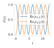
(a) Hermitian system, $\hat{H}$

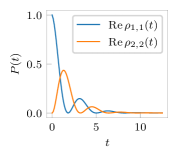
(b) Non-Hermitian system, $\hat{H}_{\text{nh}}$

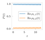
(c) Hermitian system, $\hat{H}+V(t)$

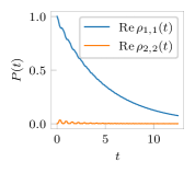
(d) Non-Hermitian system, $\hat{H}_{\text{nh}}+V(t)$

Figure 1: Dynamics of the different elements of the density matrix.

The Hamiltonian in either case can be defined as a $2\times 2$ complex matrix or by using the convenience function Utilities.create_tls_hamiltonian. Currently, QuantumDynamics.jl also provides another convenience function for creating a periodic or aperiodic nearest-neighbor Hamiltonian, Utilities.create_nn_hamiltonian.

The dynamics of a system under these two Hamiltonians starting with a density matrix of

$$\rho(0)=\begin{pmatrix}1.0&0.0\\ 0.0&0.0\end{pmatrix}.$$ (9)

is shown in Figs. 1 (a) and (b). When a time-dependent external field, $V(t)=12\cos(10t)$, is coupled with the operator $\hat{\sigma}_{z}$, the dynamics changes substantially. The dynamics under the external field for the Hermitian and non-Hermitian systems are shown in Fig. 1 (c) and (d) respectively.

The code snippet for simulating the dynamics of the non-Hermitian system in presence of the external field is as follows:

⬇

using QuantumDynamics

\par# define the Hamiltonian

H = [-0.1im -1.0; -1.0 -0.5im]

V(t) = 12 * cos(10.0 * t)

EF = Utilities.ExternalField(V, [1.0+0.0im 0.0; 0.0 -1.0])

\par# define the initial condition, the time step and the number of steps of simulation

ρ0 = [1.0+0.0im 0.0; 0.0 0.0]

dt = 0.125

ntimes = 100

\par# simulate the dynamics using the propagate method

times, ρs = Bare.propagate(; Hamiltonian=H, ρ0, dt, ntimes, external_fields=[EF])

The other cases are also similar. Notice that the Hamiltonian is defined as a simple $2\times 2$ matrix. The design moves away from defining classes hierarchies for these fundamental objects because that creates barriers when using different hardwares. For example, with the current design, implementing the same algorithm on a graphics processing unit (GPU) should be as simple as using the array abstractions in a Julia library like CUDA.jl [68]. The external field, Utilities.ExternalField, is a struct with a simple function of time and the system operator that couples to the field. The same Bare.propagate function works for Hermitian or non-Hermitian systems with or without external fields.

III.1.2 Lindblad Master Equation

Consider a system interacting with a variety of environment degrees of freedom as in Eq. 1. An empirical approach of incorporating effects of these environments on the dynamics of the reduced density matrix (RDM) of the quantum systems is through the use of the Lindblad Master Equation,

$$\derivative{\rho(t)}{t} =-\frac{i}{\hbar}\commutator{\hat{H}_{0}}{\rho(t)}+\sum_{j}\left(L_{j}\rho(t)L_{j}^{\dagger}-\frac{1}{2}\anticommutator{L_{j}^{\dagger}L_{j}}{\rho(t)}\right),$$ (10)

where $\hat{H}_{0}$ is the Hamiltonian of the system, $\rho(t)$ is the time-evolved system RDM. The impact of the environment is empirically modeled through the so-called Lindblad “jump” operators, $L_{j}$. Different processes require different types of jump operators. A couple of examples are demonstrated here.

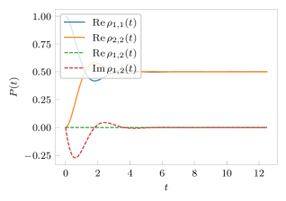
Figure 2: Simulation of dynamics corresponding to a typical spin-boson parameter.

For mapping a spin-boson problem onto a system described with the Lindblad master equation, we obtain a jump operator proportional to $\sigma_{z}$. The strength of the system-bath coupling in a spin-boson parameter is related to this proportionality constant. Consider a system Hamiltonian given by $\hat{H}_{0}=-\sigma_{x}$, and a localized initial condition. The code to simulate the dynamics using QuantumDynamics.jl is:

⬇

using QuantumDynamics

\par# define the Hamiltonian, the initial RDM, and the simulation details

H = Matrix{ComplexF64}([

0.0 -1.0

-1.0 0.0

])

ρ0 = [1.0+0.0im 0.0; 0.0 0.0]

dt = 0.125

ntimes = 100

\par# define the Lindbladian jump operator

L = [1.0+0.0im 0.0; 0.0 -1.0]

\par# call propagate with a list of jump operators to be applied

times, ρs = Bare.propagate(; Hamiltonian=H, ρ0, dt, ntimes, L=[L])

The resultant dynamics is shown in Fig. 2. One can notice the features reminiscent of a typical spin-boson parameters [3, 4]. Also note that the only change from the simulations of the isolated Hermitian and non-Hermitian systems is the new argument, L, containing a vector of jump operators $L_{j}$ that is being passed in.

Now, consider a more involved example. We want to model an excitation transport between a dimer of molecules while accounting for possibility of spontaneous emission which will bring one molecule to the ground state without exciting the other. This possibility does not allow for modeling the problem in the so-called first excitation subspace. In the full Hilbert space, the system Hamiltonian is taken to be

$$\hat{H}_{0} =20.0\outerproduct{ee}{ee}+10.0\outerproduct{ge}{ge}+10.0\outerproduct{eg}{eg}$$

$$-1.0\outerproduct{eg}{ge}-1.0\outerproduct{ge}{eg}.$$ (11)

The simulation is started from an initial condition of $\outerproduct{ge}{ge}$. For the effects of the molecular vibrations moving the energies of the excited and the ground states, we use jump operators proportional to $\sigma_{z}\otimes\mathbb{I}$ and $\mathbb{I}\otimes\sigma_{z}$. For capturing the spontaneous decay process, we introduce jump operators proportional to $\sigma_{m}\otimes\mathbb{I}$ and $\mathbb{I}\otimes\sigma_{m}$. The code for simulating this system is as follows:

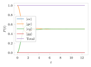
(a) Dynamics for bo=0.7071 and se=0.0.

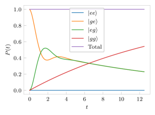
(b) Dynamics for bo=0.7071 and se=0.25.

Figure 3: Simulation of dynamics corresponding to an excitation transfer in a dimer with and without spontaneous emission.

⬇

using QuantumDynamics

\par# define Hamiltonian, initial RDM and simulation parameters

H = Matrix{ComplexF64}([

20.0 0.0 0.0 0.0

0.0 10.0 -1.0 0.0

0.0 -1.0 10.0 0.0

0.0 0.0 0.0 0.0

])

ρ0 = Matrix{ComplexF64}([

0.0 0.0 0.0 0.0

0.0 1.0 0.0 0.0

0.0 0.0 0.0 0.0

0.0 0.0 0.0 0.0

])

dt = 0.125

ntimes = 100

\par# define the jump operators corresponding to the decohering effects of the individual Born-Oppenheimer surfaces.

# bo is the coupling strength

σz = bo * Matrix{ComplexF64}([

1.0 0.0

0.0 -1.0

])

id = Matrix{ComplexF64}([

1.0 0.0

0.0 1.0

])

L1 = kron(σz, id)

L2 = kron(id, σz)

\par# define the jump operators corresponding to spontaneous emission

# se is the coupling strength

σm = se * Matrix{ComplexF64}([

0.0 0.0

1.0 0.0

])

L3 = kron(σm, id)

L4 = kron(id, σm)

\partimes, ρs = Bare.propagate(; Hamiltonian=H, ρ0, dt, ntimes, L=[L1, L2, L3, L4])

where the proportionality constants have been given as bo and se for the molecular vibrations and the spontaneous emission processes respectively. Figure 3 demonstrates the dynamics obtained using this code when spontaneous emission is switched off and on. We see the expected conservation of the number of excitation when spontaneous emission is turned off, and a gradual build up of population in the ground state in presence of spontaneous emission.

III.2 Perturbative & Non-Perturbative Dynamics of Open Quantum Systems

While QuantumDynamics.jl supports empirical methods as described in Sec. III.1, the primary focus is rigorous methods of simulation of open quantum systems. Now, we turn our attention to the more numerical involved methods. For these examples, we will specify the detailed characteristics of the harmonic bath using spectral densities.

III.2.1 Bloch-Redfield Master Equation

The Bloch-Redfield master equation [1, 2] (BRME) is one of the simplest and most versatile approaches to perturbatively simulate the dynamics of open quantum systems. It includes a perturbative description of the system-environment interaction with the environment being described under the Born approximation. Finally, an additional approximation of Markovian dynamics is invoked to obtain BRME. While the combination of approximations involved often makes the method unsuitable for strongly coupled solvents, it is still useful for understanding the very rough timescales of dynamics. Combining BRME with ideas of polaron transform is successful in extending its applicability to strongly coupled non-perturbative solvents [69, 70, 71, 72, 73].

For the system-solvent Hamiltonian, Eq. 1, under the Born approximation and Markovian limit of the environment, BRME can be expressed as an equation of motion for the reduced density matrix in the eigen-basis of the system Hamiltonian, $\hat{H}_{0}$:

$$\derivative{\rho_{ab}}{t} =-i\omega_{ab}\rho_{ab}(t)+\sum_{cd}R_{abcd}\rho_{cd}(t),$$ (12)

where $R_{abcd}$ is the Redfield tensor that captures the impact of the solvent on the system in a perturbative manner:

$$R_{abcd}=-\frac{1}{2}\sum_{k=1}^{N_{\text{env}}} \left(\delta_{bd}\sum_{n}\bra{a}\hat{s}_{k}\outerproduct{n}{n}\hat{s}_{k}\ket{c}J_{k}(\omega_{c}-\omega_{n})\right.$$

$$-\matrixelement{a}{\hat{s}_{k}}{c}\matrixelement{d}{\hat{s}_{k}}{b}J_{k}(\omega_{c}-\omega_{a})$$

$$+\delta_{ac}\sum_{n}\bra{d}\hat{s}_{k}\outerproduct{n}{n}\hat{s}_{k}\ket{b}J_{k}(\omega_{d}-\omega_{n})$$

$$-\left.\vphantom{\sum_{k=1}^{N_{\text{env}}}}\matrixelement{a}{\hat{s}_{k}}{c}\matrixelement{d}{\hat{s}_{k}}{b}J_{k}(\omega_{d}-\omega_{b})\right)$$ (13)

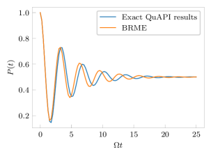
Figure 4: Comparison between BRME simulation and numerically exact QuAPI calculations. Discussion of QuAPI is given later in Sec. III.2.3.

A particular example of the results of BRME for a spin-boson system and its comparison with exact quantum dynamical calculations using QuAPI is shown in Fig. 4. The code for simulating the BRME equations using QuantumDynamics.jl for this particular case is as follows:

⬇

using QuantumDynamics

\par# define the system Hamiltonian

H = Matrix{ComplexF64}([

0.0 -1.0

-1.0 0.0

])

\par# specify the spectral density describing the bath and the inverse temperature

Jw = SpectralDensities.ExponentialCutoff(; ξ=0.1, ωc=7.5)

β = 5.0

\parρ0 = Matrix{ComplexF64}([

1.0 0.0

0.0 0.0

])

dt = 0.25

ntimes = 100

time, ρs = BlochRedfield.propagate(; Hamiltonian=H, Jw=[Jw], β, ρ0, dt, ntimes, sys_ops=[[1.0+0.0im 0.0; 0.0 -1.0]])

III.2.2 Hierarchical Equations of Motion

The hierarchical equations of motion (HEOM) [6, 74, 56, 57] is one of the two foundational numerically exact, non-perturbative methods for simulating the dynamics of an open quantum system interacting with a harmonic bath. While originally formulated primarily for the Drude-Lorentz spectral density, recent work has made it possible to use this method with more general spectral densities [75, 76, 77, 78]. Other developments have improved the numerical stability of HEOM at lower temperatures [79]. QuantumDynamics.jl supports the scaled version of HEOM [23] for the Drude-Lorentz spectral density. The more advanced approaches required to handle other spectral densities will be incorporated in later versions of the package.

The general problem that HEOM solves is Eq. 1. However, for HEOM, the system-environment interaction Hamiltonian is not exactly Eq. 2. It is given by

$$\hat{H}^{(b)}_{\text{env}} =\sum_{j}\frac{p_{jb}^{2}}{2m_{jb}}+\frac{1}{2}m_{jb}\omega_{jb}^{2}x_{jb}^{2}-c_{jb}\hat{s}_{b}x_{jb}$$ (14)

Notice that the difference with Eq. 2 is that here, the square is not completed. For the implementation of HEOM in QuantumDynamics.jl, the baths need to be characterized by spectral densities having the Drude-Lorentz form:

$$J_{b}(\omega) =\frac{2\lambda_{b}}{\Delta s_{b}^{2}}\frac{\gamma_{b}\omega}{\omega^{2}+\gamma_{b}^{2}}.$$ (15)

The separation between the system states is $\Delta s_{b}$. For problems involving exciton transport, the spectral density is specified using $\Delta s_{b}=1$. For application of HEOM, the correlation functions corresponding to the spectral densities are written in a sum over poles form [23],

$$C_{b}(t) =\sum_{m=0}^{\infty}c_{bm}\exp(-\nu_{bm}t),$$ (16)

where $\nu_{b0}=\gamma_{b}$ is the Drude decay constant and $\nu_{bm\geq 1}=2m\pi/\beta$ are the Matsubara frequencies. The coefficients $c_{bm}$ are given by

$$c_{b0} =\gamma_{b}\frac{\lambda_{b}}{\Delta s_{b}^{2}}\left(\cot\left(\frac{\beta\hbar\gamma_{b}}{2}\right)-i\right),$$ (17)

$$c_{bm\geq 1} =\frac{4\lambda_{b}\gamma_{b}}{\beta\hbar\Delta s_{b}^{2}}\left(\frac{\nu_{bm}}{\nu_{bm}^{2}-\gamma_{b}^{2}}\right).$$ (18)

For such a system, the primary expression for HEOM is given as:

$$\derivative{\rho_{\mathbf{n}}}{t} =-\frac{i}{\hbar}\commutator{\hat{H}_{0}}{\rho_{\mathbf{n}}}+\sum_{b=1}^{N_{\text{env}}}\sum_{m=0}^{M}n_{bm}\nu_{bm}\rho_{\mathbf{n}}$$

$$-\sum_{b=1}^{N_{\text{env}}}\left(\frac{2\lambda_{b}}{\beta\hbar^{2}\gamma_{b}}-\sum_{m=0}^{M}\frac{c_{bm}}{\hbar\nu_{bm}}\right)\commutator{\hat{s}_{b}}{\commutator{\hat{s}_{b}}{\rho_{\mathbf{n}}}}$$

$$-i\sum_{b=1}^{N_{\text{env}}}\commutator{\hat{s}_{b}}{\sum_{m=0}^{M}\rho_{\mathbf{n}_{bm}^{+}}}$$

$$-\frac{i}{\hbar}\sum_{b=1}^{N_{\text{env}}}\sum_{m=0}^{M}n_{bm}\left(c_{bm}\hat{s}_{b}\rho_{\mathbf{n}_{bm}^{-}}-c_{bm}^{*}\rho_{\mathbf{n}_{bm}^{-}}\hat{s}_{b}\right),$$ (19)

where $\rho_{\mathbf{n}}$ represents the generalized density operators — when $\mathbf{n}=0,0,0,\ldots$, it is the reduced density operator, for all other $\mathbf{n}$, it is an auxiliary density operator. The subscript vectors, $\mathbf{n}$ are of length $N_{\text{env}}K(M+1)$, where $K$ is the depth of the hierarchy. Each density matrix is assigned a depth of $L=\sum_{b=1}^{N_{\text{env}}}\sum_{m=0}^{M}n_{bm}$. The term in the second line of Eq. 19 is the correction term is the Ishizaki-Tanimura scheme of truncating the truncating the Matsubara terms by treating $m>M$ using a Markovian approximation [7, 8].

The scaled version of HEOM [23] rescales the auxiliary density operators in a manner that allows truncation of the hierarchy at a lower value of $K$.

$$\tilde{\rho}_{\mathbf{n}} =\left(\prod_{b}\prod_{m}n_{bm}!|c_{bm}|^{n_{bm}}\right)^{-\frac{1}{2}}\rho_{\mathbf{n}},$$ (20)

which changes Eq. 19 to:

$$\derivative{\tilde{\rho}_{\mathbf{n}}}{t} =-\frac{i}{\hbar}\commutator{\hat{H}_{0}}{\tilde{\rho}_{\mathbf{n}}}+\sum_{b=1}^{N_{\text{env}}}\sum_{m=0}^{M}n_{bm}\nu_{bm}\tilde{\rho}_{\mathbf{n}}$$

$$-\sum_{b=1}^{N_{\text{env}}}\left(\frac{2\lambda_{b}}{\beta\hbar^{2}\gamma_{b}}-\sum_{m=0}^{M}\frac{c_{bm}}{\hbar\nu_{bm}}\right)\commutator{\hat{s}_{b}}{\commutator{\hat{s}_{b}}{\tilde{\rho}_{\mathbf{n}}}}$$

$$-i\sum_{b=1}^{N_{\text{env}}}\commutator{\hat{s}_{b}}{\sum_{m=0}^{M}\sqrt{(n_{bm}+1)|c_{bm}|}\tilde{\rho}_{\mathbf{n}_{bm}^{+}}}$$

$$-\frac{i}{\hbar}\sum_{b=1}^{N_{\text{env}}}\sum_{m=0}^{M}\sqrt{\frac{n_{bm}}{|c_{bm}|}}\left(c_{bm}\hat{s}_{b}\tilde{\rho}_{\mathbf{n}_{bm}^{-}}-c_{bm}^{*}\tilde{\rho}_{\mathbf{n}_{bm}^{-}}\hat{s}_{b}\right).$$ (21)

In this new version, Eq. 21, the number of levels of hierarchy required for convergence decreases significantly in comparison to the original unscaled HEOM, Eq. 19. This is the version that is used by default in QuantumDynamics.jl. To use the unscaled version of HEOM, one needs to set scaled to false while calling the HEOM.propagate function.

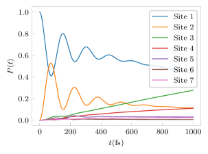
(a) $T=$77\text{\,}\mathrm{K}$$

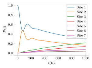
(b) $T=$300\text{\,}\mathrm{K}$$

Figure 5: Excitation population dynamics in the 7-state FMO model introduced by Ishizaki and Fleming [80].

As a demonstration of the HEOM module in the code, we simulate the dynamics of the chromophoric excitation in the famous 7-state model for the Fenna-Matthews-Olson (FMO) complex [81, 80] at $T=$77\text{\,}\mathrm{K}300\text{\,}\mathrm{K}$$. The code snippet for this part is quite self-explanatory:

⬇

using QuantumDynamics

\par# unit conversion

invcm2au = 4.55633e-6

au2fs = 0.02418884254

\parfunction FMO(num_modes, Lmax, β)

# set up the system Hamiltonian

H = Matrix{ComplexF64}([

12410 -87.7 5.5 -5.9 6.7 -13.7 -9.9

-87.7 12530 30.8 8.2 0.7 11.8 4.3

5.5 30.8 12210 -53.5 -2.2 -9.6 6.0

-5.9 8.2 -53.5 12320 -70.7 -17.0 -63.3

6.7 0.7 -2.2 -70.7 12480 81.1 -1.3

-13.7 11.8 -9.6 -17.0 81.1 12630 39.7

-9.9 4.3 6.0 -63.3 -1.3 39.7 12440

]) * invcm2au

nsteps = 500 # number of steps of simulations

dt = 1000 / au2fs / nsteps # dt for simulation

\par# initial density matrix with excitation localized on BChl unit 1

ρ0 = Matrix{ComplexF64}(zeros(7, 7))

ρ0[1, 1] = 1

\par# create spectral densities on each of the BChl sites

λs = [35.0, 35.0, 35.0, 35.0, 35.0, 35.0, 35.0] * invcm2au

γs = 1 ./ ([50.0, 50.0, 50.0, 50.0, 50.0, 50.0, 50.0] / au2fs)

Jw = Vector{SpectralDensities.DrudeLorentz}()

sys_ops = Vector{Matrix{ComplexF64}}()

for (j, (λ, γ)) in enumerate(zip(λs, γs))

push!(Jw, SpectralDensities.DrudeLorentz(; λ, γ, Δs=1.0))

op = zeros(7, 7)

op[j, j] = 1.0

push!(sys_ops, op)

end

\par# simulate the time evolution of ρ0 using HEOM

t, ρ = HEOM.propagate(; Hamiltonian=H, ρ0=ρ0, Jw, β, ntimes=nsteps, dt, sys_ops, num_modes, Lmax)

t .*= au2fs

t, ρ

end

Here, we use the propagate function under the HEOM submodule. It takes a list of spectral densities, Jw, along with the corresponding system operators that couple to a particular bath, sys_ops. The number of Matsubara modes that are required to converge the results is num_modes and Lmax is the number of auxiliary density operators considered in the calculation. At both temperatures, well converged results were obtained with num_modes $=2$ and Lmax $=3$. The dynamics obtained using this code is shown in Fig. 5 which matches the original results reported by Ishizaki and Fleming [80].

As a final example of HEOM, let us consider the case of spontaneous emission that was modelled empirically using Lindblad Master Equation, Fig. 3, in Sec. III.1.2. Spontaneous emission happens because of the presence of an environment or bath that is able to couple the molecular excited state to the molecular ground state, thereby reducing the excited state lifetime to some finite value. Once again, the ground and excited states will include the corresponding vibrations and the changes in energy that they bring about. The resultant dynamics is shown in Fig. 6. The bath which enables a spontaneous excitation or relaxation of the molecular eigenstate is acts through the system $\hat{\sigma}_{x}$ operator, whereas the baths representing the vibrational motion on the Born-Oppenheimer surfaces act through $\hat{\sigma}_{z}$. HEOM is able to handle both a “diagonal” and an “off-diagonal” bath on the same footing without an increase in computational complexity.

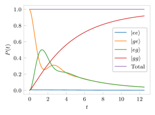
Figure 6: Dynamics of an excitonic dimer with multiple non-commuting baths.

⬇

# define Hamiltonian, initial RDM and simulation parameters

H = Matrix{ComplexF64}([

20.0 0.0 0.0 0.0

0.0 10.0 -1.0 0.0

0.0 -1.0 10.0 0.0

0.0 0.0 0.0 0.0

])

ρ0 = Matrix{ComplexF64}([

0.0 0.0 0.0 0.0

0.0 1.0 0.0 0.0

0.0 0.0 0.0 0.0

0.0 0.0 0.0 0.0

])

dt = 0.125

ntimes = 100

\par# define the spectral density for the vibrational bath

Jw = Vector{SpectralDensities.DrudeLorentz}()

svec = Vector{Matrix{ComplexF64}}()

σz = Matrix{ComplexF64}([

1.0 0.0

0.0 -1.0

])

id = Matrix{ComplexF64}([

1.0 0.0

0.0 1.0

])

jw1 = SpectralDensities.DrudeLorentz(; λ=bo, γ=5.0, Δs=1.0)

bo1 = kron(σz, id)

bo2 = kron(id, σz)

\par# define the bath that cause a change in the excitation state of a monomer

σx = Matrix{ComplexF64}([

0.0 1.0

1.0 0.0

])

jw3 = SpectralDensities.DrudeLorentz(; λ=se, γ=5.0, Δs=1.0)

se3 = kron(σx, id) + kron(id, σx)

\partimes, ρs = HEOM.propagate(; Hamiltonian=H, ρ0=ρ0, Jw=[jw1, jw1, jw3], β, ntimes, dt, sys_ops=[bo1, bo2, se3], num_modes, Lmax)

III.2.3 Path Integral Methods

Path integral approaches form the other numerically exact family of computational methods for simulating the dynamics of open quantum systems as described by Eqs. 1 and 2. Since the original papers [3, 4, 5] significant developments [10, 11, 21, 18, 17, 19, 63, 20, 15, 13, 12] have led to the proliferation of methods based on the foundations of path integrals with Feynman-Vernon influence functional [9].

Starting from an initial state given as a direct product of the system reduced density matrix and the thermal distribution of the environment, the dynamics of the system after $N$ time-steps can be expressed as a path integral,

$$\matrixelement{s_{N}^{+}}{\rho(N\Delta t)}{s_{N}^{-}} =\sum_{s_{0}^{\pm}}\sum_{s_{1}^{\pm}}\ldots\sum_{s_{N-1}^{\pm}}\bra{s_{N}^{+}}\hat{U}\outerproduct{s_{N-1}^{+}}{s_{N-1}^{+}}\hat{U}\ket{s_{N-2}^{+}}\ldots$$

$$\times\bra{s_{1}^{+}}\hat{U}\outerproduct{s_{0}^{+}}{s_{0}^{+}}\rho(0)\outerproduct{s_{0}^{-}}{s_{0}^{-}}\hat{U}^{\dagger}\ket{s_{1}^{-}}\ldots\bra{s_{N-1}^{-}}\hat{U}\ket{s_{N}^{-}}F[\{s^{\pm}_{j}\}]$$ (22)

$$\text{where }F[\{s^{\pm}_{j}\}] =\exp\left(-\frac{1}{\hbar}\sum_{k=0}^{N}(s_{k}^{+}-s_{k}^{-})\sum_{k^{\prime}=0}^{k}(\eta_{kk^{\prime}}s_{k^{\prime}}^{+}-\eta^{*}_{kk^{\prime}}s_{k^{\prime}}^{-})\right).$$ (23)

Here, $\hat{U}$ is the bare system propagator, and $F$ is the Feynman-Vernon influence functional corresponding to the forward-backward path $s^{\pm}_{j}$. The influence functional for a system coupled to multiple environments is given as a product of the influence functionals corresponding to the individual environments. The cost of simulations do not increase as long as all the operators that the environments couple to commute with each other. The bath response function is discretized into $\eta$-coefficients [3]. The non-Markovian nature of the dynamics is brought in by the dependence of the influence functional on the full path of the system. However, in condensed phases, the memory decays away with the time difference of the interacting points. Thus, after a full-memory simulation of $L$ time steps, which is a convergence parameter, one can use an iterative algorithm to propagate the reduced density matrix further out in time. The summand of the right-hand side of Eq. 22 can be thought of as a tensor indexed by the forward-backward system paths called the path amplitude tensor.

Various approaches have been used to reduce the computational complexity of the problem which naïvely grows as $\mathcal{O}(d^{2L})$ where $d$ is the system dimensionality and $L$ is the memory length. This is the original QuAPI algorithm. Other approaches attempt to decrease this exponentially growing computational and storage requirements. The blip decomposition [10, 11] of path integral uses the fact that the influence functional, Eq. 23, depends on the value of $\Delta s=s^{+}-s^{-}$ for the latter point. That means that for all the paths with no time-point where $\Delta s=0$ the influence functional is one. Thus this set of paths can be summed up in a Markovian manner. In fact, any segment of path that consists solely of points with $\Delta s=0$, or “sojourns”, can be summed up through iterative matrix-vector multiplications thereby reducing the effective number of paths that need to be considered.

Recently tensor networks have been used in a variety of ways to reduce the complexity of these path integral calculations. Most prominent of these is the time-evolved matrix product operators approach [21] (TEMPO) which uses a matrix product state to give a compact represent the path amplitude tensor utilizing the decaying correlation between indices with large separation. Under the tensor network path integral [15] (TNPI) implementation of the TEMPO algorithm, it has been shown that the influence functional for multiple baths can be analytically represented in the form of an optimal matrix product operator. Additionally, PC-TNPI is a new tensor network that has been designed to manifestly capture the symmetries present in the influence functional [12].

There are four basic modules of path integral simulations that are supported — QuAPI implementing ideas in Refs. [3, 4], Blip implementing Ref. [10], TEMPO implemeting Ref. [21], and PCTNPI implementing Ref. [12]. In principle iterative propagation of reduced density matrices beyond the memory time is possible in all of these methods, however based on our experience, of these methods TEMPO gives the greatest ability to access long memory lengths and large systems. Thus iterative propagation is implemented only in TEMPO and in base QuAPI. All the modules support creation of augmented propagators which are the effective propagators of the system in presence of the solvent.

First, we demonstrate the QuantumDynamics.jl code both for the most fundamental path integral method, QuAPI [3, 4] and for TEMPO [21]. Consider the symmetric system, $\hat{H}_{0}=-\hbar\Omega\sigma_{x}$ coupled with a bath of harmonic oscillators characterized by an Ohmic spectral density where $\xi$ is the dimensionless Kondo parameter and $\omega_{c}$ is the cutoff frequency. The simulation with any of the methods will have the following outline:

⬇

# define the system Hamiltonian

H = Matrix{ComplexF64}([

0.0 -1.0

-1.0 0.0

])

\par# calculate the sequence of bare propagators with a given time-step

barefbU = Propagators.calculate_bare_propagators(; Hamiltonian=H, dt, ntimes)

\par# define the initial condition and the spectral density

ρ0 = [1.0+0.0im 0.0; 0.0 0.0]

Jw = SpectralDensities.ExponentialCutoff(; ξ, ωc)

\par# use a given method to propagate the initial state in presence of the environment at an inverse temperature, β.

# method is one of QuAPI.propagate or TEMPO.propagate

t, ρs = method(; fbU=barefbU, Jw=[Jw], β, ρ0, dt, ntimes, L, svec)

method is currently one of QuAPI.propagate or TEMPO.propagate. These propagate methods take custom extra arguments which specify how to tune the algorithms in specific ways to improve the performance.

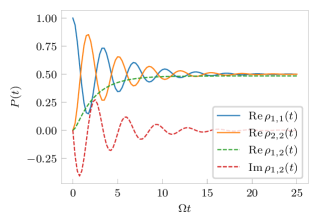
(a) $\xi=0.1$, $\omega_{c}=7.5\Omega$, $\hbar\Omega\beta=5$, $L=6$, $\Delta t=0.25$. Parameters from Ref. [3]. Run with method=QuAPI.propagate.

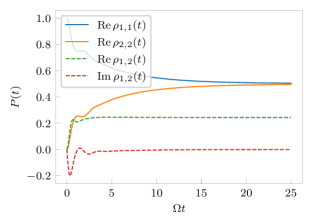
(b) $\xi=2.0$, $\omega_{c}=\Omega$, $\hbar\Omega\beta=1$, $L=150$, $\Delta t=0.125$. Parameters from Ref. [63, 82]. Run with method=TEMPO.propagate.

Figure 7: Example of dynamics using QuAPI-related methods simulated using QuantumDynamics.jl.

As an illustration, we demonstrate two different parameters using base QuAPI (Fig. 7 (a)) and using TEMPO (Fig. 7 (b)). For the example simulated using QuAPI, we use a parameter that was introduced in Ref. [3]. For the example that we simulated using TEMPO, we chose a parameter that was originally simulated using quantum-classical path integral up to a short time [82] and more recently using SMatPI till equilibration [63]. For this case, the bath is localized around the initial system state.

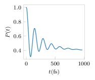
(a) $\lambda=$20\text{\,}{\mathrm{cm}}^{-1}$$

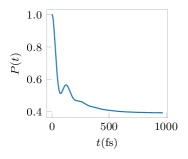
(b) $\lambda=$100\text{\,}{\mathrm{cm}}^{-1}$$

Figure 8: Simulation of a excitation energy transfer dimer with parameters obtained from Ref. [83]. $\epsilon=$100\text{\,}{\mathrm{cm}}^{-1}$$, $\Omega=$-100\text{\,}{\mathrm{cm}}^{-1}$$.

For problems where the iterative portion of the dynamics is significantly longer than the full-memory portion, the cost of the iteration, which is proportional to the number of paths, adds up. One way of solving this is to use TTM [62] to reduce the cost to a “convolution” of these transfer tensors and the augmented propagators. TTM uses the other base path integral methods to generate the propagators for some number of time-steps and then uses them calculate the propagators further out in time. We demonstrate the use of TTM using the strongly excitation energy transfer (EET) dimer from Ref. [83]. The structure of a code using TTM is shown below:

⬇

# define the EET dimer Hamiltonian

H = Matrix{ComplexF64}([

50 100.0

100.0 -50

] .* invcm2au)

# using a time-step, dt, calculate the bare forward-backward propagators for ntimes time-steps

fbU = Propagators.calculate_bare_propagators(; Hamiltonian=H, ntimes, dt)

\par# define the spectral densities acting on the different monomers

J1 = SpectralDensities.DrudeLorentz(; λ=λ * invcm2au, γ=γ * invcm2au, Δs=1.0)

J2 = SpectralDensities.DrudeLorentz(; λ=λ * invcm2au, γ=γ * invcm2au, Δs=1.0)

svec = [1.0 0.0; 0.0 1.0]

β = 1052.0

\parρ0 = [1.0+0.0im 0.0; 0.0 0.0]

# TTM.propagate takes a particular path_integral_routine and the corresponding extraargs.

times, ρs = TTM.propagate(; fbU=fbU, ρ0=ρ0, Jw=[J1, J2], β, ntimes, dt, svec, rmax=rmax, extraargs=TEMPO.TEMPOArgs(; cutoff=1e-13, maxdim=10000), path_integral_routine = TEMPO.build_augmented_propagator, verbose=true)

These calculations were done with full memory simulations of 75 steps with a time-step of $\Delta t=$4.84\text{\,}\mathrm{fs}$$. The spectral density used is the Drude-Lorentz spectral density, Eq. 5, with $\gamma=$53.08\text{\,}{\mathrm{cm}}^{-1}$$. The results are shown for two different reorganization energies, $\lambda$, are shown in Fig. 8.

Finally, the last major method supported by QuantumDynamics.jl is QCPI [58, 59] with reference propagators [60] and harmonic backreaction [61]. The incorporation of classical trajectories not only allows for larger time-steps but also reduces the effective memory that needs to be accounted for through path integrals by incorporating the classical part of the memory completely [60]. A simulation that only incorporates the classical part of the memory is called the ensemble average classical path (EACP) simulation. With reference propagators one can do this simulation in a Markovian manner. Currently the support is only for a harmonic bath though the infrastructure is built in such a manner that it is trivial to extend it to include anharmonic solvents in the reference propagators either by solving the equations of motion using DifferentialEquations.jl [64], or couple it with a molecular dynamics frameworks like Molly.jl and the Atomic Simulation Engine [84] (ASE). Due to the modular nature of QuantumDynamics.jl, these different classical trajectory backends will work in a plug-and-play manner.

Below is a code snippet which does both the EACP calculation and a full QCPI calculation on a sample spin-boson parameter.

⬇

# specify the system Hamiltonian

H0 = Matrix{ComplexF64}([

1.0 -1.0

-1.0 -1.0

])

\par# specify the spectral density and the inverse temperature

Jw = SpectralDensities.ExponentialCutoff(; ξ=0.1, ωc=7.5)

β = 5.0

\parρ0 = Matrix{ComplexF64}([

1.0 0.0

0.0 0.0

])

\pardt = 0.25

ntimes = 100

\par# discretize the spectral density and create a harmonic bath solvent

# for an atomistic solvent, here we would use the actual description based on an appropriate force field or ab initio DFT calculation

ω, c = SpectralDensities.discretize(Jw, 100)

hb = Solvents.HarmonicBath(β, ω, c, [1.0, -1.0], num_points)

\par# calculate EACP dynamics

EACP_fbU = Propagators.calculate_average_reference_propagators(; Hamiltonian=H0, solvent=hb, classical_dt=dt / 100, dt, ntimes)

times_EACP, ρs_EACP = Utilities.apply_propagator(; propagators=EACP_fbU, ρ0, ntimes, dt)

\par# simulate QCPI

times_QCPI, ρs_QCPI = QCPI.propagate(; Hamiltonian=H0, Jw, solvent=hb, ρ0, classical_dt=dt / 100, dt, ntimes, kmax=3, extraargs=QuAPI.QuAPIArgs(), path_integral_routine=QuAPI.propagate)

QuantumDynamics.jl does not enforce any parallelization over the Monte Carlo runs or binning and calculation of error statistics. That is left to the end user to implement in a manner suited to the problem being studied. It will be quite simple to spread QCPI.propagate calls over multiple nodes and aggregate across them using message-passing interface. The dynamics obtained with 10000 initial conditions is demonstrated in Fig. 9.

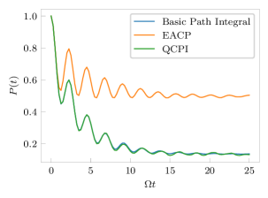
Figure 9: Comparison between QuAPI and QCPI runs for the parameters shown in the code. 10000 initial conditions were used for the EACP and QCPI calculations.

IV Conclusion

In this paper, we have introduced a new package called QuantumDynamics.jl for simulations of non-adiabatic processes using the Feynman-Vernon influence functional [9]. The Julia programming language has been emerging as a promising candidate for modern high-level high-performance scientific computing, with a growing base of packages for computational chemistry and physics. Being written in Julia, allows QuantumDynamics.jl to take advantage of packages like DifferentialEquations.jl for solving differential equations. This also allows us to avoid the “two-language” problem where the performance critical parts need to be implemented in some lower-level high-performance language.

Simulating the dynamics of quantum systems interacting with environments is often very difficult if done in a numerically exact manner. The exact methods are quite involved from a theoretical perspective while being challenging to implement in code. They are built on top of a variety of deep insights into the structure of dynamics in these systems. Very few open-source packages exist that aim to make these methods accessible to non-specialists while providing for a platform to the specialists that encourages explorations and further theoretical development. Inspired by the objectives behind PySCF [30], QuantumDynamics.jl was designed to address this particular problem. It joins the recently growing ranks of computational packages for chemistry in the Julia programming language [44, 42, 45].

QuantumDynamics.jl already supports a variety of methods. On the empirical and perturbative end, methods like propagation of non-Hermitian Hamiltonians, Lindblad master equation, and the perturbative Bloch-Redfield master equation are all built on top of the backend provided DifferentialEquations.jl. BRME can later be extended using polaron and variational polaron transformed approaches to increase the applicability of the perturbative ideas. In terms of numerically exact approaches, both HEOM-based and QuAPI-based methods are supported. In HEOM, we have already implemented the unscaled and scaled version. Use of matrix product states and other approaches of generalizing it to account for non-Drude-Lorentz spectral densities will be implemented in the near future.

The largest set of methods implemented in QuantumDynamics.jl fall in the category of path integral- or QuAPI-based approaches. The base methods of QuAPI, blip decomposition, TEMPO, and PC-TNPI are all supported. QuAPI and TEMPO support propagation of density matrices, while blips and PC-TNPI are currently only capable of producing augmented forward-backward propagators. While this does not hamper the usability of these methods in conjunction with TTM, this deficiency will be remedied in a future version. Probably the single most useful sub-module of the path integral methods is TEMPO. Given its ability to handle comparatively large systems with long memories makes it exceptionally powerful. The TNPI-based implementation allows use of multiple baths in an optimal manner. The compatibility of all of these methods with TTM is a very useful feature of QuantumDynamics.jl.

The goal is to provide the community with a platform that is fit for exploration and method development in addition to a repository of methods that can directly be used for accurate simulations of quantum dynamics. There are many other developments that are yet to be incorporated in QuantumDynamics.jl. A notable example is the recently developed multisite decomposition of the tensor network path integral [13] (MS-TNPI), which combines ideas from time-dependent density matrix renormalization group [85, 86, 87, 88, 89] with the Feynman-Vernon influence functional in order to make simulations of extended open quantum systems feasible [90, 91]. While we will introduce some methods like MS-TNPI [13] in the near future and continue to develop into this package, we hope that QuantumDynamics.jl becomes a toolbox for the community with others actively using and developing it as well.

References

- Bloch [1957] F. Bloch, Generalized Theory of Relaxation, Phys. Rev. 105, 1206 (1957).
- Redfield [1957] A. G. Redfield, On the Theory of Relaxation Processes, IBM J. Res. Dev. 1, 19 (1957).
- Makri and Makarov [1995a] N. Makri and D. E. Makarov, Tensor propagator for iterative quantum time evolution of reduced density matrices. I. Theory, The Journal of Chemical Physics 102, 4600 (1995a).
- Makri and Makarov [1995b] N. Makri and D. E. Makarov, Tensor propagator for iterative quantum time evolution of reduced density matrices. II. Numerical methodology, The Journal of Chemical Physics 102, 4611 (1995b).
- Makri [1995] N. Makri, Numerical path integral techniques for long time dynamics of quantum dissipative systems, Journal of Mathematical Physics 36, 2430 (1995).
- Tanimura and Kubo [1989] Y. Tanimura and R. Kubo, Time Evolution of a Quantum System in Contact with a Nearly Gaussian-Markoffian Noise Bath, Journal of the Physical Society of Japan 58, 101 (1989).
- Ishizaki and Tanimura [2005] A. Ishizaki and Y. Tanimura, Quantum Dynamics of System Strongly Coupled to Low-Temperature Colored Noise Bath: Reduced Hierarchy Equations Approach, J. Phys. Soc. Jpn. 74, 3131 (2005).
- Tanimura [2006] Y. Tanimura, Stochastic Liouville, Langevin, Fokker–Planck, and Master Equation Approaches to Quantum Dissipative Systems, J. Phys. Soc. Jpn. 75, 082001 (2006).
- Feynman and Vernon [1963] R. P. Feynman and F. L. Vernon, The theory of a general quantum system interacting with a linear dissipative system, Annals of Physics 24, 118 (1963).
- Makri [2014] N. Makri, Blip decomposition of the path integral: Exponential acceleration of real-time calculations on quantum dissipative systems, The Journal of Chemical Physics 141, 134117 (2014).
- Makri [2017] N. Makri, Iterative blip-summed path integral for quantum dynamics in strongly dissipative environments, The Journal of Chemical Physics 146, 134101 (2017).
- Bose [2022a] A. Bose, Pairwise connected tensor network representation of path integrals, Physical Review B 105, 024309 (2022a).
- Bose and Walters [2022a] A. Bose and P. L. Walters, A multisite decomposition of the tensor network path integrals, The Journal of Chemical Physics 156, 024101 (2022a).
- Makri [2018] N. Makri, Modular path integral methodology for real-time quantum dynamics, The Journal of Chemical Physics 149, 214108 (2018).
- Bose and Walters [2021] A. Bose and P. L. Walters, A tensor network representation of path integrals: Implementation and analysis, arXiv pre-print server arXiv:2106.12523 (2021), arxiv:2106.12523 .
- Jørgensen and Pollock [2019] M. R. Jørgensen and F. A. Pollock, Exploiting the Causal Tensor Network Structure of Quantum Processes to Efficiently Simulate Non-Markovian Path Integrals, Physical Review Letters 123, 240602 (2019).
- Makri [2020a] N. Makri, Small matrix disentanglement of the path integral: Overcoming the exponential tensor scaling with memory length, The Journal of Chemical Physics 152, 41104 (2020a).
- Makri [2020b] N. Makri, Small Matrix Path Integral for System-Bath Dynamics, Journal of Chemical Theory and Computation 16, 4038 (2020b).
- Makri [2021a] N. Makri, Small matrix modular path integral: Iterative quantum dynamics in space and time, Physical Chemistry Chemical Physics 23, 12537 (2021a).
- Makri [2021b] N. Makri, Small matrix path integral for driven dissipative dynamics, The Journal of Physical Chemistry A 125, 10500 (2021b), https://doi.org/10.1021/acs.jpca.1c08230 .
- Strathearn et al. [2018] A. Strathearn, P. Kirton, D. Kilda, J. Keeling, and B. W. Lovett, Efficient non-Markovian quantum dynamics using time-evolving matrix product operators, Nature Communications 9, 10.1038/s41467-018-05617-3 (2018).
- Hu et al. [2011] J. Hu, M. Luo, F. Jiang, R.-X. Xu, and Y. Yan, Padé spectrum decompositions of quantum distribution functions and optimal hierarchical equations of motion construction for quantum open systems, J. Chem. Phys. 134, 244106 (2011).
- Shi et al. [2009] Q. Shi, L. Chen, G. Nan, R.-X. Xu, and Y. Yan, Efficient hierarchical Liouville space propagator to quantum dissipative dynamics, J. Chem. Phys. 130, 084105 (2009).
- Shi et al. [2018] Q. Shi, Y. Xu, Y. Yan, and M. Xu, Efficient propagation of the hierarchical equations of motion using the matrix product state method, The Journal of Chemical Physics 148, 174102 (2018).
- Yan et al. [2021] Y. Yan, M. Xu, T. Li, and Q. Shi, Efficient propagation of the hierarchical equations of motion using the Tucker and hierarchical Tucker tensors, The Journal of Chemical Physics 154, 194104 (2021).
- Ikeda and Scholes [2020] T. Ikeda and G. D. Scholes, Generalization of the hierarchical equations of motion theory for efficient calculations with arbitrary correlation functions, The Journal of Chemical Physics 152, 204101 (2020).
- Aprà et al. [2020] E. Aprà, E. J. Bylaska, W. A. de Jong, N. Govind, K. Kowalski, T. P. Straatsma, M. Valiev, H. J. J. van Dam, Y. Alexeev, J. Anchell, V. Anisimov, F. W. Aquino, R. Atta-Fynn, J. Autschbach, N. P. Bauman, J. C. Becca, D. E. Bernholdt, K. Bhaskaran-Nair, S. Bogatko, P. Borowski, J. Boschen, J. Brabec, A. Bruner, E. Cauët, Y. Chen, G. N. Chuev, C. J. Cramer, J. Daily, M. J. O. Deegan, T. H. Dunning, M. Dupuis, K. G. Dyall, G. I. Fann, S. A. Fischer, A. Fonari, H. Früchtl, L. Gagliardi, J. Garza, N. Gawande, S. Ghosh, K. Glaesemann, A. W. Götz, J. Hammond, V. Helms, E. D. Hermes, K. Hirao, S. Hirata, M. Jacquelin, L. Jensen, B. G. Johnson, H. Jónsson, R. A. Kendall, M. Klemm, R. Kobayashi, V. Konkov, S. Krishnamoorthy, M. Krishnan, Z. Lin, R. D. Lins, R. J. Littlefield, A. J. Logsdail, K. Lopata, W. Ma, A. V. Marenich, J. Martin del Campo, D. Mejia-Rodriguez, J. E. Moore, J. M. Mullin, T. Nakajima, D. R. Nascimento, J. A. Nichols, P. J. Nichols, J. Nieplocha, A. Otero-de-la-Roza, B. Palmer, A. Panyala, T. Pirojsirikul, B. Peng, R. Peverati, J. Pittner, L. Pollack, R. M. Richard, P. Sadayappan, G. C. Schatz, W. A. Shelton, D. W. Silverstein, D. M. A. Smith, T. A. Soares, D. Song, M. Swart, H. L. Taylor, G. S. Thomas, V. Tipparaju, D. G. Truhlar, K. Tsemekhman, T. Van Voorhis, Á. Vázquez-Mayagoitia, P. Verma, O. Villa, A. Vishnu, K. D. Vogiatzis, D. Wang, J. H. Weare, M. J. Williamson, T. L. Windus, K. Woliński, A. T. Wong, Q. Wu, C. Yang, Q. Yu, M. Zacharias, Z. Zhang, Y. Zhao, and R. J. Harrison, NWChem: Past, present, and future, J. Chem. Phys. 152, 184102 (2020).
- Frisch et al. [2016] M. J. Frisch, G. W. Trucks, H. B. Schlegel, G. E. Scuseria, M. A. Robb, J. R. Cheeseman, G. Scalmani, V. Barone, G. A. Petersson, H. Nakatsuji, X. Li, M. Caricato, A. V. Marenich, J. Bloino, B. G. Janesko, R. Gomperts, B. Mennucci, H. P. Hratchian, J. V. Ortiz, A. F. Izmaylov, J. L. Sonnenberg, Williams, F. Ding, F. Lipparini, F. Egidi, J. Goings, B. Peng, A. Petrone, T. Henderson, D. Ranasinghe, V. G. Zakrzewski, J. Gao, N. Rega, G. Zheng, W. Liang, M. Hada, M. Ehara, K. Toyota, R. Fukuda, J. Hasegawa, M. Ishida, T. Nakajima, Y. Honda, O. Kitao, H. Nakai, T. Vreven, K. Throssell, J. A. Montgomery Jr., J. E. Peralta, F. Ogliaro, M. J. Bearpark, J. J. Heyd, E. N. Brothers, K. N. Kudin, V. N. Staroverov, T. A. Keith, R. Kobayashi, J. Normand, K. Raghavachari, A. P. Rendell, J. C. Burant, S. S. Iyengar, J. Tomasi, M. Cossi, J. M. Millam, M. Klene, C. Adamo, R. Cammi, J. W. Ochterski, R. L. Martin, K. Morokuma, O. Farkas, J. B. Foresman, and D. J. Fox, Gaussian 16 Rev. C.01 (2016).
- Smith et al. [2020] D. G. A. Smith, L. A. Burns, A. C. Simmonett, R. M. Parrish, M. C. Schieber, R. Galvelis, P. Kraus, H. Kruse, R. Di Remigio, A. Alenaizan, A. M. James, S. Lehtola, J. P. Misiewicz, M. Scheurer, R. A. Shaw, J. B. Schriber, Y. Xie, Z. L. Glick, D. A. Sirianni, J. S. O’Brien, J. M. Waldrop, A. Kumar, E. G. Hohenstein, B. P. Pritchard, B. R. Brooks, H. F. Schaefer, A. Y. Sokolov, K. Patkowski, A. E. DePrince, U. Bozkaya, R. A. King, F. A. Evangelista, J. M. Turney, T. D. Crawford, and C. D. Sherrill, PSI4 1.4: Open-source software for high-throughput quantum chemistry, J. Chem. Phys. 152, 184108 (2020).
- Sun et al. [2018] Q. Sun, T. C. Berkelbach, N. S. Blunt, G. H. Booth, S. Guo, Z. Li, J. Liu, J. D. McClain, E. R. Sayfutyarova, S. Sharma, S. Wouters, and G. K.-L. Chan, PySCF: The Python-based simulations of chemistry framework, WIREs Computational Molecular Science 8, e1340 (2018).
- Balasubramani et al. [2020] S. G. Balasubramani, G. P. Chen, S. Coriani, M. Diedenhofen, M. S. Frank, Y. J. Franzke, F. Furche, R. Grotjahn, M. E. Harding, C. Hättig, A. Hellweg, B. Helmich-Paris, C. Holzer, U. Huniar, M. Kaupp, A. Marefat Khah, S. Karbalaei Khani, T. Müller, F. Mack, B. D. Nguyen, S. M. Parker, E. Perlt, D. Rappoport, K. Reiter, S. Roy, M. Rückert, G. Schmitz, M. Sierka, E. Tapavicza, D. P. Tew, C. van Wüllen, V. K. Voora, F. Weigend, A. Wodyński, and J. M. Yu, TURBOMOLE: Modular program suite for ab initio quantum-chemical and condensed-matter simulations, J. Chem. Phys. 152, 184107 (2020).
- Kühne et al. [2020] T. D. Kühne, M. Iannuzzi, M. Del Ben, V. V. Rybkin, P. Seewald, F. Stein, T. Laino, R. Z. Khaliullin, O. Schütt, F. Schiffmann, D. Golze, J. Wilhelm, S. Chulkov, M. H. Bani-Hashemian, V. Weber, U. Borštnik, M. Taillefumier, A. S. Jakobovits, A. Lazzaro, H. Pabst, T. Müller, R. Schade, M. Guidon, S. Andermatt, N. Holmberg, G. K. Schenter, A. Hehn, A. Bussy, F. Belleflamme, G. Tabacchi, A. Glöß, M. Lass, I. Bethune, C. J. Mundy, C. Plessl, M. Watkins, J. Vandevondele, M. Krack, and J. Hutter, CP2K: An electronic structure and molecular dynamics software package - Quickstep: Efficient and accurate electronic structure calculations, The Journal of Chemical Physics 152, 194103 (2020).
- Giannozzi et al. [2009] P. Giannozzi, S. Baroni, N. Bonini, M. Calandra, R. Car, C. Cavazzoni, D. Ceresoli, G. L. Chiarotti, M. Cococcioni, I. Dabo, A. Dal Corso, S. de Gironcoli, S. Fabris, G. Fratesi, R. Gebauer, U. Gerstmann, C. Gougoussis, A. Kokalj, M. Lazzeri, L. Martin-Samos, N. Marzari, F. Mauri, R. Mazzarello, S. Paolini, A. Pasquarello, L. Paulatto, C. Sbraccia, S. Scandolo, G. Sclauzero, A. P. Seitsonen, A. Smogunov, P. Umari, and R. M. Wentzcovitch, QUANTUM ESPRESSO: A modular and open-source software project for quantum simulations of materials, Journal of Physics: Condensed Matter 21, 395502 (2009).
- Giannozzi et al. [2017] P. Giannozzi, O. Andreussi, T. Brumme, O. Bunau, M. Buongiorno Nardelli, M. Calandra, R. Car, C. Cavazzoni, D. Ceresoli, M. Cococcioni, N. Colonna, I. Carnimeo, A. Dal Corso, S. de Gironcoli, P. Delugas, R. A. DiStasio, A. Ferretti, A. Floris, G. Fratesi, G. Fugallo, R. Gebauer, U. Gerstmann, F. Giustino, T. Gorni, J. Jia, M. Kawamura, H.-Y. Ko, A. Kokalj, E. Küçükbenli, M. Lazzeri, M. Marsili, N. Marzari, F. Mauri, N. L. Nguyen, H.-V. Nguyen, A. Otero-de-la-Roza, L. Paulatto, S. Poncé, D. Rocca, R. Sabatini, B. Santra, M. Schlipf, A. P. Seitsonen, A. Smogunov, I. Timrov, T. Thonhauser, P. Umari, N. Vast, X. Wu, and S. Baroni, Advanced capabilities for materials modelling with Quantum ESPRESSO, Journal of Physics: Condensed Matter 29, 465901 (2017).
- Kapil et al. [2019] V. Kapil, M. Rossi, O. Marsalek, R. Petraglia, Y. Litman, T. Spura, B. Cheng, A. Cuzzocrea, R. H. Meißner, D. M. Wilkins, B. A. Helfrecht, P. Juda, S. P. Bienvenue, W. Fang, J. Kessler, I. Poltavsky, S. Vandenbrande, J. Wieme, C. Corminboeuf, T. D. Kühne, D. E. Manolopoulos, T. E. Markland, J. O. Richardson, A. Tkatchenko, G. A. Tribello, V. Van Speybroeck, and M. Ceriotti, I-PI 2.0: A universal force engine for advanced molecular simulations, Computer Physics Communications 236, 214 (2019).
- [36] C. Kreisbeck and T. Kramer, Exciton dynamics lab for light-harvesting complexes (GPU-HEOM), 2013, See nanohub. org for electronic tool, doi: https://doi. org/10.4231/D3RB6W248 .
- Strümpfer and Schulten [2012] J. Strümpfer and K. Schulten, Open Quantum Dynamics Calculations with the Hierarchy Equations of Motion on Parallel Computers, J. Chem. Theory Comput. 8, 2808 (2012).
- Tsuchimoto and Tanimura [2015] M. Tsuchimoto and Y. Tanimura, Spins Dynamics in a Dissipative Environment: Hierarchal Equations of Motion Approach Using a Graphics Processing Unit (GPU), J. Chem. Theory Comput. 11, 3859 (2015).
- Temen et al. [2020] S. Temen, A. Jain, and A. V. Akimov, Hierarchical equations of motion in the Libra software package, International Journal of Quantum Chemistry 120, e26373 (2020).
- Johansson et al. [2013] J. Johansson, P. Nation, and F. Nori, QuTiP 2: A Python framework for the dynamics of open quantum systems, Computer Physics Communications 184, 1234 (2013).
- Akimov [2016] A. V. Akimov, Libra: An open-source “methodology discovery” library for quantum and classical dynamics simulations, Journal of Computational Chemistry 37, 1626 (2016).
- Gardner et al. [2022] J. Gardner, O. A. Douglas-Gallardo, W. G. Stark, J. Westermayr, S. M. Janke, S. Habershon, and R. J. Maurer, NQCDynamics.jl: A Julia package for nonadiabatic quantum classical molecular dynamics in the condensed phase, The Journal of Chemical Physics 156, 174801 (2022), https://doi.org/10.1063/5.0089436 .
- Bezanson et al. [2017] J. Bezanson, A. Edelman, S. Karpinski, and V. B. Shah, Julia: A fresh approach to numerical computing, SIAM Review 59, 65 (2017).
- Aroeira et al. [2022] G. J. R. Aroeira, M. M. Davis, J. M. Turney, and H. F. Schaefer, Fermi.jl: A Modern Design for Quantum Chemistry, Journal of Chemical Theory and Computation 18, 677 (2022).
- Herbst et al. [2021] M. F. Herbst, A. Levitt, and E. Cancès, DFTK: A Julian approach for simulating electrons in solids, Proc. JuliaCon Conf. 3, 69 (2021).
- Krämer et al. [2018] S. Krämer, D. Plankensteiner, L. Ostermann, and H. Ritsch, QuantumOptics.jl: A Julia framework for simulating open quantum systems, Computer Physics Communications 227, 109 (2018).
- Poole et al. [2020] D. Poole, J. L. Galvez Vallejo, and M. S. Gordon, A New Kid on the Block: Application of Julia to Hartree–Fock Calculations, J. Chem. Theory Comput. 16, 5006 (2020).
- Poole et al. [2022] D. Poole, J. L. Galvez Vallejo, and M. S. Gordon, A Task-Based Approach to Parallel Restricted Hartree–Fock Calculations, J. Chem. Theory Comput. 18, 2144 (2022).
- Makri [1999] N. Makri, The Linear Response Approximation and Its Lowest Order Corrections: An Influence Functional Approach, The Journal of Physical Chemistry B 103, 2823 (1999).
- Allen et al. [2016] T. C. Allen, P. L. Walters, and N. Makri, Direct Computation of Influence Functional Coefficients from Numerical Correlation Functions, Journal of Chemical Theory and Computation 12, 4169 (2016).
- Walters et al. [2017] P. L. Walters, T. C. Allen, and N. Makri, Direct determination of discrete harmonic bath parameters from molecular dynamics simulations, Journal of Computational Chemistry 38, 110 (2017).
- Bose [2022b] A. Bose, Zero-cost corrections to influence functional coefficients from bath response functions, The Journal of Chemical Physics 157, 054107 (2022b).
- Tully [1990] J. C. Tully, Molecular dynamics with electronic transitions, The Journal of Chemical Physics 93, 1061 (1990).
- Tully [2012] J. C. Tully, Perspective: Nonadiabatic dynamics theory, The Journal of Chemical Physics 137, 22A301 (2012).
- Wang et al. [2016] L. Wang, A. Akimov, and O. V. Prezhdo, Recent Progress in Surface Hopping: 2011–2015, J. Phys. Chem. Lett. 7, 2100 (2016).
- Tanimura [2014] Y. Tanimura, Reduced hierarchical equations of motion in real and imaginary time: Correlated initial states and thermodynamic quantities, The Journal of Chemical Physics 141, 044114 (2014), https://doi.org/10.1063/1.4890441 .
- Tanimura [2020] Y. Tanimura, Numerically “exact” approach to open quantum dynamics: The hierarchical equations of motion (HEOM), The Journal of Chemical Physics 153, 20901 (2020).
- Lambert and Makri [2012a] R. Lambert and N. Makri, Quantum-classical path integral. I. Classical memory and weak quantum nonlocality, The Journal of Chemical Physics 137, 22A552 (2012a).
- Lambert and Makri [2012b] R. Lambert and N. Makri, Quantum-classical path integral. II. Numerical methodology, The Journal of Chemical Physics 137, 22A553 (2012b).
- Banerjee and Makri [2013] T. Banerjee and N. Makri, Quantum-Classical Path Integral with Self-Consistent Solvent-Driven Reference Propagators, The Journal of Physical Chemistry B 117, 13357 (2013).
- Wang and Makri [2019] F. Wang and N. Makri, Quantum-classical path integral with a harmonic treatment of the back-reaction, The Journal of Chemical Physics 150, 184102 (2019).
- Cerrillo and Cao [2014] J. Cerrillo and J. Cao, Non-Markovian Dynamical Maps: Numerical Processing of Open Quantum Trajectories, Phys. Rev. Lett. 112, 110401 (2014).
- Makri [2021c] N. Makri, Small Matrix Path Integral with Extended Memory, Journal of Chemical Theory and Computation 17, 1 (2021c).
- Rackauckas and Nie [2017] C. Rackauckas and Q. Nie, Differentialequations.jl–a performant and feature-rich ecosystem for solving differential equations in julia, Journal of Open Research Software 5, 15 (2017).
- Tsitouras [2011] Ch. Tsitouras, Runge–Kutta pairs of order 5(4) satisfying only the first column simplifying assumption, Computers & Mathematics with Applications 62, 770 (2011).
- Fishman et al. [2022a] M. Fishman, S. White, and E. Stoudenmire, The ITensor Software Library for Tensor Network Calculations, SciPost Phys. Codebases , 4 (2022a).
- Fishman et al. [2022b] M. Fishman, S. White, and E. Stoudenmire, Codebase release 0.3 for ITensor, SciPost Phys. Codebases , 4 (2022b).
- Besard et al. [2018] T. Besard, C. Foket, and B. De Sutter, Effective extensible programming: Unleashing Julia on GPUs, IEEE Transactions on Parallel and Distributed Systems 10.1109/TPDS.2018.2872064 (2018), arxiv:1712.03112 [cs.PL] .
- Silbey and Harris [1984] R. Silbey and R. A. Harris, Variational calculation of the dynamics of a two level system interacting with a bath, The Journal of Chemical Physics 80, 2615 (1984).
- Xu and Cao [2016] D. Xu and J. Cao, Non-canonical distribution and non-equilibrium transport beyond weak system-bath coupling regime: A polaron transformation approach, Frontiers of Physics 11, 110308 (2016).
- Xu et al. [2016] D. Xu, C. Wang, Y. Zhao, and J. Cao, Polaron effects on the performance of light-harvesting systems: A quantum heat engine perspective, New Journal of Physics 18, 023003 (2016).
- Jang [2022] S. J. Jang, Partially polaron-transformed quantum master equation for exciton and charge transport dynamics, J. Chem. Phys. 157, 104107 (2022).
- Lee et al. [2012] C. K. Lee, J. Moix, and J. Cao, Accuracy of second order perturbation theory in the polaron and variational polaron frames, J. Chem. Phys. 136, 204120 (2012).
- Tanimura and Wolynes [1991] Y. Tanimura and P. G. Wolynes, Quantum and classical Fokker-Planck equations for a Gaussian-Markovian noise bath, Physical Review A 43, 4131 (1991).
- Duan et al. [2017] C. Duan, Q. Wang, Z. Tang, and J. Wu, The study of an extended hierarchy equation of motion in the spin-boson model: The cutoff function of the sub-Ohmic spectral density, The Journal of Chemical Physics 147, 164112 (2017).
- Popescu et al. [2015] B. Popescu, H. Rahman, and U. Kleinekathöfer, Using the Chebychev expansion in quantum transport calculations, J. Chem. Phys. 142, 154103 (2015).
- Tian and Chen [2013] H. Tian and G. Chen, Application of hierarchical equations of motion (HEOM) to time dependent quantum transport at zero and finite temperatures, The European Physical Journal B 86, 411 (2013).
- Liu et al. [2014] H. Liu, L. Zhu, S. Bai, and Q. Shi, Reduced quantum dynamics with arbitrary bath spectral densities: Hierarchical equations of motion based on several different bath decomposition schemes, J. Chem. Phys. 140, 134106 (2014).
- Dunn et al. [2019] I. S. Dunn, R. Tempelaar, and D. R. Reichman, Removing instabilities in the hierarchical equations of motion: Exact and approximate projection approaches, J. Chem. Phys. 150, 184109 (2019).
- Ishizaki and Fleming [2009a] A. Ishizaki and G. R. Fleming, Theoretical examination of quantum coherence in a photosynthetic system at physiological temperature, Proceedings of the National Academy of Sciences 106, 17255 (2009a).
- Adolphs and Renger [2006] J. Adolphs and T. Renger, How Proteins Trigger Excitation Energy Transfer in the FMO Complex of Green Sulfur Bacteria, Biophysical Journal 91, 2778 (2006).
- Walters and Makri [2016] P. L. Walters and N. Makri, Iterative quantum-classical path integral with dynamically consistent state hopping, The Journal of Chemical Physics 144, 44108 (2016).
- Ishizaki and Fleming [2009b] A. Ishizaki and G. R. Fleming, Unified treatment of quantum coherent and incoherent hopping dynamics in electronic energy transfer: Reduced hierarchy equation approach, The Journal of Chemical Physics 130, 234111 (2009b).
- Hjorth Larsen et al. [2017] A. Hjorth Larsen, J. Jørgen Mortensen, J. Blomqvist, I. E. Castelli, R. Christensen, M. Dułak, J. Friis, M. N. Groves, B. Hammer, C. Hargus, E. D. Hermes, P. C. Jennings, P. Bjerre Jensen, J. Kermode, J. R. Kitchin, E. Leonhard Kolsbjerg, J. Kubal, K. Kaasbjerg, S. Lysgaard, J. Bergmann Maronsson, T. Maxson, T. Olsen, L. Pastewka, A. Peterson, C. Rostgaard, J. Schiøtz, O. Schütt, M. Strange, K. S. Thygesen, T. Vegge, L. Vilhelmsen, M. Walter, Z. Zeng, and K. W. Jacobsen, The atomic simulation environment—a Python library for working with atoms, Journal of Physics: Condensed Matter 29, 273002 (2017).
- White and Feiguin [2004] S. R. White and A. E. Feiguin, Real-Time Evolution Using the Density Matrix Renormalization Group, Physical Review Letters 93, 076401 (2004).
- Schollwöck [2005] U. Schollwöck, The density-matrix renormalization group, Reviews of Modern Physics 77, 259 (2005).
- Schollwöck [2011a] U. Schollwöck, The density-matrix renormalization group in the age of matrix product states, Annals of Physics 326, 96 (2011a).
- Schollwöck [2011b] U. Schollwöck, The density-matrix renormalization group: A short introduction, Philosophical Transactions of the Royal Society A: Mathematical, Physical and Engineering Sciences 369, 2643 (2011b).
- Paeckel et al. [2019] S. Paeckel, T. Köhler, A. Swoboda, S. R. Manmana, U. Schollwöck, and C. Hubig, Time-evolution methods for matrix-product states, Annals of Physics 411, 167998 (2019).
- Bose and Walters [2022b] A. Bose and P. L. Walters, Effect of temperature gradient on quantum transport, Physical Chemistry Chemical Physics 24, 22431 (2022b).
- Bose and Walters [2022c] A. Bose and P. L. Walters, Tensor Network Path Integral Study of Dynamics in B850 LH2 Ring with Atomistically Derived Vibrations, Journal of Chemical Theory and Computation 18, 4095 (2022c).