Style Miner: Find Significant and Stable Explanatory Factors in Time Series with Constrained Reinforcement Learning

Abstract

In high-dimensional time-series analysis, it is essential to have a set of key factors (namely, the style factors) that explain the change of the observed variable. For example, volatility modeling in finance relies on a set of risk factors, and climate change studies in climatology rely on a set of causal factors. The ideal low-dimensional style factors should balance significance (with high explanatory power) and stability (consistent, no significant fluctuations). However, previous supervised and unsupervised feature extraction methods can hardly address the tradeoff. In this paper, we propose Style Miner, a reinforcement learning method to generate style factors. We first formulate the problem as a Constrained Markov Decision Process with explanatory power as the return and stability as the constraint. Then, we design fine-grained immediate rewards and costs and use a Lagrangian heuristic to balance them adaptively. Experiments on real-world financial data sets show that Style Miner outperforms existing learning-based methods by a large margin and achieves a relatively 10% gain in R-squared explanatory power compared to the industry-renowned factors proposed by human experts.

1 Introduction

As is known to all, feature extraction is crucial for data analysis and machine learning in the real world. Generally speaking, features have two major functions: for prediction and for explanation. Nowadays, predictive features can be extracted efficiently with a great number of tools in the supervised machine learning toolbox, and made a great deal of progress in many areas, including computer vision Ping Tian and others (2013), neural machine translation Bahdanau et al. (2015), and so on. However, there still remain some real-world problems where the future observations are hard to predict, such as the equity market and climate change. In these circumstances, it is more important to find the factors that have strong explanatory power so that the complex real-world states can be abstracted and thus can be understood by people. For instance, economists Ilmanen (2012) use low-dimensional style factors to explain asset volatility to understand the market, measure asset risks, and establish portfolios. Meteorologists Hegerl and Zwiers (2011); Bindoff et al. (2013) use greenhouse gas, other anthropogenic stressors, and natural components to explain the observed global surface temperature changes so the global warming can be mitigated by controlling the main style factors. In this paper, we would like to answer the question of how to use reinforcement learning to find explanatory style factors especially in high-dimensional time-series problems, which explain the observations rather than predict them, as illustrated in Figure 1.

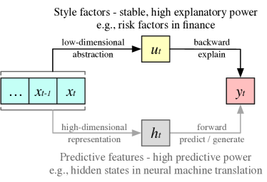
Figure 1: Comparison between style and predictive factors.

As discussed in Menchero et al.[2011], high-quality style factors should meet two basic requirements: have high explanatory power, and be stable. First, the main usage of styles is to explain the future outcomes, and the explanation should be significant. Second, styles must be stable (have little fluctuation) so that historically lagged explanations can be valuable for the future decisions. In this paper, we focus on finding style factors that meet both requirements.

There are three lines of studies for style factor extraction, which are 1) case-by-case studies by human experts, 2) unsupervised feature extraction methods, and 3) supervised feature extraction methods. The design of expert factors Guy. (1975); Sheikh (1996); Sharpe (1964) usually requires strong expertise in specific areas and can achieve reasonable performance. However, in the area of high-dimensional big data, finding new style factors in novel datasets gets harder and harder. Unsupervised methods such as principal components analysis (PCA) Wold et al. (1987) and AutoEncoder Gu et al. (2021) can find hidden variables in static datasets. However, they do not show promising performance in time-series data when the purpose is to explain unobserved future outcomes rather than current observations. Supervised learning methods, on the other hand, can handle sequential datasets with the recent progress of sequential neural networks. For example, Deep Risk Model (DRM) Lin et al. (2021) is shown to perform better than expert factors. However, as supervised deep learning methods rely on differentiable loss functions, they are hard to apply to problems with non-differentiable feedback. There are also some studies using Reinforcement Learning method in other finance domain Pan et al. (2022), however, it cannot be directly applied to style factor mining.

In this paper, we propose Style Miner, a style factor extraction method based on constrained reinforcement learning which explicitly addresses the tradeoff between explanatory power and stability. We first formulate the style factor extraction as a Constrained Markov Decision Process (CMDP) Altman (1999), where an agent tries to generate continuous style factors given the time-series observations. For each generated style factor, the agent receives the explanatory power as the long-term return and the negative autocorrelation of the factor sequence as the cost. The agent’s goal is to maximize the explanatory power while satisfying the constraint of having a high sequence autocorrelation. Further, to accelerate the training, we also propose several practical techniques to simplify the problem and an adaptive heuristic to explicitly balance the reward and the constraint. Experiments in real-world financial market data show that Style Miner can achieve state-of-the-art performance while being stable given only the raw market data inputs, which achieves a relatively 10% higher R-squared explanatory power compared to expert factors.

The main contributions of this thesis are summarized as follows:

• We propose Style Miner which extracts style factors with Constrained Reinforcement Learning. It tries to maximize the explanatory power while constraining the stability. To the best of our knowledge, it is the first study that use reinforcement learning method to extract style factors.

• We design fine-grained immediate rewards and costs to alleviate the sparse reward problem, and then use a Lagrangian heuristic to adaptively balance between the reward and the cost constraint.

• We conduct extensive experiments and show that our method can achieve state-of-the-art explanatory power with high temporal stability, which significantly outperforms the industry-renowned expert-designed factors.

2 Related Work

2.0.1 Style Factors by Human Experts

The earliest Mean-Variance Model believed the risk should be measured while considering the return. And this risk is measured by the volatility of asset returns. The stocks with higher volatility of returns usually have a higher risk. It was the first time that mathematical statistics were introduced into portfolio theory, which built the foundation for modern finance. With the Mean-Variance Model proposed, scholars have gradually realized the importance of measuring portfolio risk. The CAPM divides the risk into systematic risk and unsystematic risk. And the unsystematic risk should not be compensated by high returns. The CAPM only uses one factor to measure the systematic risk. Due to the limited explanatory power of a single factor, the Multi-Factor Model approach was proposed. The Multi-Factor Model attributes the stock’s return to several different style factors and uses those factors to estimate the covariance matrix. The main advantage of factor-based methods is to extract high-dimensional stock features into lower-dimensional factors so that the complexity of the problem will not change due to the number of stocks. The most classic method in the Multi-Factor Models is Fama-French Fama and French (1993). The Fama-French added value and size factors based on CAPM estimated the risk premium of the factors and tested the model’s performance through time-series regression. In Fama and MacBeth[1973], another cross-section regression factor model is proposed to determine the factor return at that cross-section regression. The Fama and French[2020] pointed out that the cross-section method is better. Barra is a well-known cross-section regression multi-factor model.

The above methods designed by the experts have high explanatory power, but the development is relatively slow due to the manual design requiring lots of human resources. It has spent almost decades from CAPM to Barra.

2.0.2 Unsupervised Feature Extraction Methods

Unsupervised machine learning has also been widely used in recent years. A simple and effective unsupervised method uses PCA to compress the high-dimensional stock data to the low-dimensional factor loading on the entire sequence. However, the factor loading generated by such a method does not change over time. As the stock distribution is unstable, the effect on the test set will gradually deteriorate. Therefore, Kelly et al.[2019] proposed a linear model of Instrumented PCA (IPCA), which estimates the factor load coefficient of style factor and assets from stock data. IPCA considers the asset characteristics as a variable, and the time changes can be included too. In addition, the decomposition process of Singular Value Decomposition (SVD) Golub and Reinsch (1971) can also be implemented by AutoEncoder. However, this method does not use the temporal information of the stock data. Therefore, the FactorVAE Duan et al. (2022) is based on AutoEncoder adding Gated Recurrent Unit (GRU) Cho et al. (2014) to obtain the temporal information. But FactorVAE mainly focuses on the prediction ability of the model rather than the explanatory power.

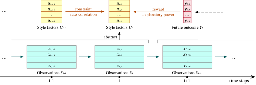
Figure 2: The overview of style factor extraction.

2.0.3 Supervised Feature Extraction Method

Supervised deep learning performs well in extracting complex non-linear features. It can also effectively use a supervised gradient to achieve the expected target. In DRM Lin et al. (2021), style factors are used as input, and GRU and Graph Attention Network (GAT) Velickovic et al. (2018) are added to discover the temporal and cross-section information. DRM designed a Multi-task method to smooth the output factors. DRM is a good attempt at deep learning in style factor extraction. However, Multi-task learning reduces training efficiency and hurts explanatory power because it is too concerned about long-term stability. Therefore, DRM has only relative increased by 2.0% compared to the expert factors. In addition, DRM uses expert factors as input which leads to original information being lost, and its results largely depend on the quality of expert factors.

3 Style Mining as a CMDP

3.1 Notations

As shown in Figure 2, consider a time-series $\{X_{{t}}\}_{t=1}^{T}$, where $X_{{t}}=\{x_{{i,t}}\}_{i=1}^{n}$ has $n$ separate observations. For each $i=1,\dots,n$, the observation $x_{{i,t}}$ is a multi-dimensional vector. Further, let $Y_{{t}}=g(X_{{{\geq t}}})$ be a future outcome for step $t$, which is the target label that we need to use the style factors to explain. And the $Y_{{t}}=\{y_{{i,t}}\}_{i=1}^{n}$ , where $y_{{i,t}}$ is a value.

Such a setting is applicable in many areas. For example, in quantitative finance, $X_{{t}}$ represents the market data at time-step $t$, $n$ is the number of stocks, $x_{{i,t}}$ represents the raw observation of the $i$-th stock at time $t$, and $Y_{{t}}$ can be the future returns or realized volatilities of these stocks.

Now, we need to find a set of style factors as a compressed representation of the historical data, denoted by $U_{{t}}=\{u_{{i,t}}\}^{n}_{i=1}=\pi(X_{{\leq t}})$, where $u_{{i,t}}\in\mathbb{R}^{K}$ is the $K$-dimensional style factor for the $i$-th sequence. It is desired that these style factors can have strong explanatory power towards the target label $Y_{{t}}$ (i.e., a stock’s styles can explain its future return), and also be stable across time as well (i.e., a stock’s styles do not change in a short time). So we need to define the following two evaluation metrics.

3.2 Evaluation Criteria of Style Factors

3.2.1 Explanatory power

At each time step, suppose the true outcomes $Y_{{t}}$ are obtained, we can fit an explanatory model $\varphi(U_{{t}})$ over the style factors, i.e.,

$$Y_{{t}}=\hat{Y_{{t}}}+\epsilon_{{t}}=\varphi(U_{{t}})+\epsilon_{{t}},$$ (1)

where $\epsilon_{{t}}=(\epsilon_{{1,t}},\dots,\epsilon_{{n,t}})$ are the unexplained residuals. Usually, we can view the proportion of explained variance as explanatory power. Specifically, in this paper we use an averaged step-wise $R^{2}$ as the metric, i.e.,

$$\textrm{Expl}(U_{{1:T}})=\sum_{t=1}^{T}R^{2}_{t}=\sum_{t=1}^{T}\bigg{[}1-\frac{\sum^{n}_{i=1}w_{{i,t}}\,\epsilon_{{i,t}}^{2}}{\sum^{n}_{i=1}w_{{i,t}}\,y_{{i,t}}^{2}}\bigg{]},$$ (2)

where $w_{{i,t}}$ is weight of the $i$-th sequence.

3.2.2 Stability

On the other hand, the style factors themselves as time-series should not fluctuate too much, which can be evaluated by the autocorrelation of the style series. Specifically, we use the lag-1 autocorrelation as follows:

$$\textrm{AutoCorr}(U_{{1:T}})=\frac{1}{K}\sum_{k=1}^{K}\textrm{Corr}\big{(}U_{{1:T-1}}^{(k)},U_{{2:T}}^{(k)}\big{)},$$ (3)

where $\textrm{Corr}(\cdot,\cdot)$ is the Pearson correlation function.

As suggested by Menchero et al.[2011], style factors are considered high quality if they have autocorrelation coefficients above 0.9, otherwise too unstable to use. Therefore, in this paper we let $\textrm{AutoCorr}(U_{{1:T}})\geq 0.9$ as a constraint for stability.

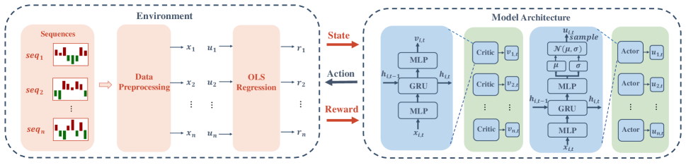
Figure 3: The overview design of Style Miner.

3.3 Constrained Markov Decision Process

We formulate the problem as a finite-horizon Constrained Markov Decision Process (CMDP) Altman (1999), i.e.,

$$\max_{\pi\in\Pi}\mathbb{E}_{\tau\sim\pi}[\mathcal{R}(U_{{1:T}})],$$ (4)

$$\operatorname{s.t.} \mathbb{E}_{\tau\sim\pi}\left[\mathcal{C}(U_{{1:T}})\right]\leq d_{0},$$

where $\mathcal{M}=\langle S,U,\mathcal{P},\mathcal{R},\mathcal{C},d_{0}\rangle$, where $S_{{t}}$ is the state space which contain the history observation, $U$ is the action space, $\mathcal{P}$ is a transition function, $\mathcal{R}$ is the reward function, $\mathcal{C}$ is the cost function, and $d_{0}\in\mathbb{R}_{+}$ is the maximum allowed cost. With trajectory $\tau:=(S_{{0}},U_{{0}},S_{{1}},\dots)$, where $U_{{t}}\sim\pi(\cdot|S_{{t}}),S_{{t+1}}\sim P(\cdot|S_{{t}},U_{{t}})$, we use the explanatory power as the reward and stability as the constraint, i.e.,

$$\mathcal{R}(U_{{1:T}})={\textrm{Expl}(U_{{1:T}})},$$ (5)

$$\mathcal{C}(U_{{1:T}})={1-\textrm{AutoCorr}(U_{{1:T}})}.$$

4 The Style Miner Algorithm

There are two major challenges for the problem:

1. How to simplify the raw problem which has high problem complexity but sparse feedback.

2. How to design an algorithm to efficiently balance the tradeoff between significance and stability.

4.1 Simplify the CMDP with Hidden States and Immediate Feedbacks

From the previous section, we see that the problem has high-dimensional observations and actions but also has very few feedback signals. It is known that such a sparse reward problem can be hard to optimize. Therefore, in this section, we simplify the problem with three techniques: 1) the hidden state technique from sequential modelling to turn the high-dimensional sequential input into dense hidden representations, 2) representation for each sequence , and 3) the immediate rewards and costs to alleviate the sparse reward problem.

The details of the simplified CMDP are describe as following:

4.1.1 Simplified states

There are two sources of complexity in the raw observations $S_{{t}}=\{X_{{\leq t}}\}$: 1) it includes $N$ multi-variable sequences, and $N$ can be large; 2) it includes $t$ historical time-steps, and $t$ can be large. Therefore, we suggest a simplified state setting with an independent encoder structure. We first decompose the overall state into individual sequences $S_{{t}}=\big{\{}\{x_{{i,t}}\}_{t}\big{\}}^{n}_{i=1}$ and assume an encoder that generates hidden states for each individual sequence $h_{{i,t}}=\textrm{Encoder}(s_{{i,t}})$, so that $\tilde{s}_{i,t}=(x_{{i,t}},h_{{i,t-1}})$.

Although not equivalent to the original problem definition, in this way the agent can take all the sequences as mini-batches and make decisions in parallel, which can empirically yields reasonable performance in practical problems.

4.1.2 Immediate rewards

In the original setting, as the backward explanation and evaluation step takes all the sample sequences into account, every sequence shares the same cumulative return $\mathcal{R}(U_{1:T})$. To make full use of the minibatch-based policy iteration, we would like to distinguish the contribution of each individual sample sequence. Therefore, at each time step $t$, we decompose the overall R-squared $R_{t}^{2}$ into fine-grained immediate rewards for all the sequences. The $i$-th sequence gets the following reward:

$$r_{i,t}=\frac{1}{n}-\frac{w_{{i,t}}u_{{i,t}}^{2}}{\sum^{n}_{i=1}w_{{i,t}}y_{{i,t}}^{2}}.$$ (6)

So that we still have $r_{t}=R_{t}^{2}=\sum_{i=1}^{N}r_{i,t}$.

4.1.3 Costs

For each sequence $i$, the overall cost function is $\mathcal{C}(u_{{i,1:T}})=1-\textrm{AutoCorr}(u_{{i,1:T}})$. As this cost can only be obtained after the episode is done, we define the immediate cost for each time-step $t$ as follows:

$$\begin{split}c(u_{i,t})=\left\{\begin{array}[]{ll}\mathcal{C}(u_{i,1:T}),&\text{if}\quad t=T\\ 0,&\text{otherwise}\end{array}\right..\end{split}$$ (7)

4.2 Policy Optimization with Stability Constrain

Based on the CMDP described above, we use Proximal Policy Optimization (PPO) Schulman et al. (2017) to optimize a policy $\pi$. PPO is an on-policy RL algorithm based on the trust region method, and it is applicable to continuous decision-making problems. It proposed a clipped version surrogate objective as follows:

$$L_{i,t}(\theta)=\min\left(\alpha_{i,t}(\theta)\hat{A}_{i,t},\textrm{clip}\left(\alpha_{t}(\theta),1-\epsilon,1+\epsilon\right)\hat{A}_{i,t}\right),$$ (8)

where $\alpha_{i,t}(\theta)=\frac{\pi_{\theta}(u_{{i,t}}|s_{{i,t}})}{\pi_{old}(u_{{i,t}}|s_{{i,t}})}$, and the $\pi_{old}$ is the old policy before update, and $\hat{A}_{i,t}$ is the estimated advantage calculated as follow:

$$\hat{A}_{i,t}=\sum^{k-1}_{j\geq 0}{\lambda^{j}\delta_{i,t+j}},$$ (9)

where $\delta_{i,t}=r_{i,t}+V(s_{{i,t+1}})-V(s_{{i,t}})$ and $\lambda$ is a discount coefficient to balance future errors.

A common approach to solving a CMDP problem is using the Lagrange relaxation technique Altman (1999). The Lagrange relaxation technique can turn the CMDP into an equivalent unconstrained problem by adding a penalty term, making the optimization process feasible.

However, in Style Miner, we found that our problem does not need to ensure that the constraints are met from beginning to end during the training process, but only the final result needs to meet the constraint. Therefore, we use a simpler heuristic method. Like the Lagrange approaches, it turns constraint into a regularization term with an adaptive multiplier $\beta$. The multiplier has a linear increasing schedule, i.e, $\beta^{\prime}=\min(\beta+\Delta\beta,\beta_{\max})$, until the constraint is met. Therefore, the surrogate loss can be formed as:

$$\begin{split}L^{Actor}_{i,t}=&\hat{\mathbb{E}}_{i,t}\bigg{[}\min\left(\alpha_{i,t}(\theta)\hat{A}_{i,t},\textrm{clip}\left(\alpha_{i,t}(\theta),1-\epsilon,1+\epsilon\right)\hat{A}_{i,t}\right)\\ &-\beta\max((c(u_{{i,t}})-d_{0}),0)\bigg{]}.\end{split}$$ (10)

After that, within the feasible solution range, Style Miner will optimize the explanatory power objective function in the unconstrained state. Therefore, this simple heuristic guarantees that Style Miner will finally achieve the constraints while optimizing the objective.

The loss function of the critic network is the mean-square-error between the output of critic network and the empirical value of cumulative future rewards $V_{i,t}^{target}$:

$$L^{Critic}_{i,t}=\mathbb{E}_{i,t}\left[\left(V(s_{{i,t}})-V^{target}_{i,t}\right)^{2}\right],$$ (11)

where $V^{target}_{i,t}$ can be calculate as follows:

$$V^{target}_{i,t}=\sum_{t^{\prime}>t}r_{i,t^{\prime}}.$$ (12)

Algorithm 1 Training Procedure for Style Miner

Input: inital policy parameters $\theta$, initial value function parameters $\phi$

1:  for each episode do

2:     for each $t$ do

3:        Generate style factors $u_{{i,t}}=\pi_{\theta}(s_{{i,t}})$

4:        Obtain the next state $s_{{i,t+1}}$ and the reward $r_{i,t}$

5:        Store the transition $\tau=(s_{{i,t}},u_{{i,t}},r_{i,t},s_{{i,t+1}})$

6:     end for

7:     Compute cumulative future rewards $V^{target}_{i,t}$ according Eq. (12)

8:     Compute advantage estimates $\hat{A}_{t}$ according Eq. (9) based on the current value function

9:     Divide episode into data chunks

10:     Update the policy parameter $\theta$ to maximize the surrogate objective in Eq. (10) for each data chunk via stochastic gradient ascent with Adam

11:     Update the value function parameter $\phi$ according Eq. (11)

12:     if the constraint is satisfy then

13:        Deactivate the constraint penalty and stop update $\beta$

14:     else

15:        if the constraint is satisfied before then

16:           Activate the constraint penalty but not update $\beta$

17:        else

18:           Update $\beta$

19:        end if

20:     end if

21:  end for

4.2.1 The Style Miner Framework

The entire framework of Style Miner can be found in Figure 3. Based on the actor-critic framework, we add the GRU both in Actor and Critic to obtain the hidden temporal information. We choose GRU due to it is simple and effective. The GRU architecture can be formulated as follows:

$$h_{{i,t}} =\textrm{LayerNorm}(\textrm{GRU}(x_{{i,t}},h_{{i,t-1}})).$$ (13)

The parameter $\theta$ of actor and critic between different sequences are shared.

During training, following the original PPO Schulman et al. (2017), the action is obtained by an action distribution, where the mean and variance from the policy output so the policy can achieve exploration. Each episode has the same length, which is the length of the training dataset. After each episode terminates, the policy will update $k$ epochs. Different from PPO, we divide the entire episode into data trunks so we can train these data trunks in parallel and keep the original order in each data trunk.

After the update, we will calculate the autocorrelation of the new policy on the validation dataset. Since it is time-consuming to calculate the autocorrelation of all stocks, we will sample dozens of stocks to get an approximate estimate. Once the autocorrelation meets the constraint, we will stop to increase the coefficient $\beta$.

The coefficient $\beta_{\max}$ is used to control the increased speed of the penalty term of constraint. $d_{0}$ is the constrained term. Now we present our new algorithm, Style Miner, as shown in Algorithm 1, and all sequences are executed in parallel.

5 Experiments

Our experiments are based on style factor extraction on three datasets from the Chinese stock market with raw market data and expert-designed features. Through the experiments, we would like to answer three questions:

Q1: Whether Style Miner can generate style factors with both high explanatory power and high stability?

Q2: Can we explicitly control the trade-off between them?

Q3: How about the performance of Style Miner with different features and different datasets?

Q4: How dose each part effect the performance of Style Miner?

5.1 Experiment settings

5.1.1 Data

Our experiments are conducted on original raw data from the Chinese stock market. For the main experiments, we choose 13 commonly used raw features as the input:{open, high, low, close, VWAP (Volume-Weighted Average Price), volume, money, negMarketValue, turnover rate, amount of transactions, PB, PE, percent-change}. The dataset splits are based on datetimes (2013/10/28 to 2017/12/29 for training, 2018/01/02 to 2018/12/28 for validation, and 2019/01/02 to 2019/12/30 for test). Furthermore, we also train our algorithm on two datasets including CSI500, and CSI1000, to test the robustness and practicality of generated factors.

5.1.2 Compared Methods

We organize and reproduce the existing style factor mining methods in detail, including expert factors Menchero et al. (2011), unsupervised learning methods Wold et al. (1987); Gu et al. (2021); Kelly et al. (2019) and supervised learning methods Lin et al. (2021). In addition to several classical style factor generation methods currently available in the quantitative field, we have also implemented several reinforcement learning methods for comparison, including PPO Schulman et al. (2017), DDPG Lillicrap et al. (2016) and TD3 Fujimoto et al. (2018). A detail description of each baseline and hyperparameter of Style Miner can be found in Appendix. We set the factor dimensions of all baselines equal to ten for a fair comparison.

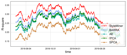
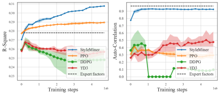
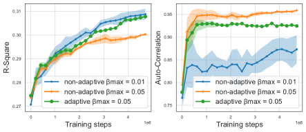
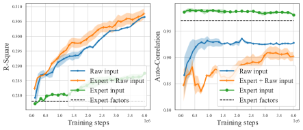
Figure 4: Experiments results. The solid lines are averaged cumulative regrets over three random seeds, and the shaded areas stand for the standard deviations. (a) The R-square of different algorithms on the test set (60 days moving averages). (b) The comparison between different RL methods on valid dataset. (c) The comparison between different $\beta_{\max}$. (d) The comparison between different input features.

5.1.3 Data Preprocessing

The price columns (open, high, low, close, and VWAP) have similar values, so we replace high, low, close, and VWAP with the percent changes relative to the open price. All feature columns are standardized with Z-scores. In addition, we used forward fill to handle the missing values.

5.1.4 Evalutation Metrics

We choose three metrics as follow:

• $\mathbf{R^{2}}$ is used to measures the explanatory power of model. The calculation of $R^{2}$ is defined as Eq. (2).

• Avg. T-value is the average absolute t-statistic of all style factors. The T-value shows the significant of the style factors.

• AutoCorr is the average of the autocorrelation coefficients of all factors over all stock series. The calculation of autocorrelation is defined as Eq. (3).

The above three metrics are all the higher, the better.

5.2 Experiment Results

5.2.1 Main Results

To answer Q1, we first compared several well-established baseline models with Style Miner on three major metrics: $R^{2}$, Average T-value of all factors, and AutoCorr. The environment is based on the full stocks with its raw data, and the results are calculated on the test dataset.

Algorithms	$R^{2}$	Avg. T-value	AutoCorr
ExpertFactors	24.8%	2.89	0.97
PCA	19.1%	0.85	-
IPCA	23.8%	4.11	0.29
AutoEncoder	23.1%	3.32	0.21
PPO	25.4%	2.16	0.39
DDPG	24.5%	2.71	0.22
TD3	24.7%	2.57	0.33
StyleMiner	27.4%	4.43	0.92
StyleMiner (post-EMA)	26.5%	3.81	0.98
StyleMiner (Expert input)	25.6%	2.71	0.99
StyleMiner (Expert+Raw input)	27.6%	4.38	0.93

Table 1: The performance of the compared algorithms.

The results are shown in Table 1. Under the premise of using raw data as input, Style Miner can achieve a 10.4% relative gain in $R^{2}$ than the expert factors with the AutoCorr above 0.92, which satisfies the stability requirement. The PCA method has no Autocorr since it is fixed values on the entire series.

For the situation that needs to achieve a higher AutoCorr, we also provide an Exponential Moving Average (EMA) version of Style Miner, i.e., using a simple weighted average over the generated sequence of style factors. The EMA can be formulated as $U_{{t}}=\rho U_{{t}}+(1-\rho)U_{{t-1}}$, here we set $\rho=0.25$. Since the style factors generated by Style Miner already have high stability, it can achieve an extremely high AutoCorr with less $R^{2}$ lost. The final result of the EMA version of Style Miner with daily features can still relatively exceed 6.4% $R^{2}$ than the expert factors with the same AutoCorr. And the $R^{2}$ of each day on the validation and test dataset is shown in Figure 4. It can be seen that on the entire validation and test set, Style Miner can achieve a far better explanatory power than the current public methods.

To answer the Q2, we compared the performance of Style Miner without adaptive penalty, which means the penalty term will keep affecting the policy even if the constraint is met. As shown in Fig. 4, Style Miner with adaptive $\beta_{\max}=0.05$ can achieve a nearly $R^{2}$ to non-adaptive $\beta_{\max}=0.01$ and still keep a high autocorrelation.

5.2.2 Comparison with Supervised Learning Method

We reproduce Deep Risk Model(DRM), which is a supervised learning method, and make detailed comparisons with Style Miner in Table. 2. The parameter H is the horizon of multi-task learning in DRM. The larger the H, the smoother the model output. The experimental results are shown in Table 2.

Algorithms	$R^{2}$	Avg. T-value	AutoCorr
ExpertFactors	24.8%	2.89	0.97
DRM (H =  1, Raw)	26.4%	4.36	0.20
DRM (H = 20, Raw)	24.6%	3.49	0.57
DRM (H =  1, Expert)	25.0%	2.64	0.98
DRM (H = 20, Expert)	25.0%	2.74	0.99
DRM (H =  1, Raw + Expert)	27.4%	3.88	0.56
DRM (H = 20, Raw + Expert)	25.6%	3.48	0.70
StyleMiner (Raw)	27.4%	4.43	0.92
StyleMiner (Raw + EMA)	26.5%	3.81	0.98
StyleMiner (Expert)	25.6%	2.71	0.99
StyleMiner (Expert+Raw)	27.6%	4.38	0.93

Table 2: The performance of the compared algorithms.

By comparing different types of input data, we can find that DRM has higher requirements for input data, and in the case of raw data input, DRM cannot obtain high stability. So the multi-task learning method in DRM can not promise stability and will lead to the problems of slow training speed and poor explanatory power. In addition, under the same input, Style Miner can obtain explanatory power and stability far exceeding DRM.

5.2.3 Comparison with Reinforcement Learning Methods

The training curves of all RL-based methods are shown in Figure 4. Although the other reinforcement learning methods can mine style factors with close explanatory power to expert factors, the generated style factors are unstable.

5.2.4 Different Input Features and Datasets

We further investigate the performance of Style Miner with different features (Q3). As shown in Figure 4, when using expert factors as input, the model will achieve a high autocorrelation due to the input being quite stable. However, the explanatory power is also limited due to the smooth input. By using both raw data and expert factors as input, Style Miner can achieve a higher $R^{2}$ with autocorrelation above 0.9. Therefore, we can conclude that with smoother input features, Style Miner can obtain a higher interpretation ratio while maintaining higher stability. Additional input features can further help improve the explanatory power of the model.

We also test two datasets from the Chinese stock market, including CSI500 and CSI1000, which contain 500 and 1000 stocks. We show CSI500 in Table 3, CSI1000 and the time cost of Style Miner and PPO on three datasets can be found in Appendix. The results show that, since the scale of stocks is decreasing, the output of other models has also become more stable but still does not meet the requirements (Above 0.9).

Algorithms	$R^{2}$	AutoCorr
StyleMiner	31.1%	0.92
PPO	28.7%	0.75
DDPG	28.0%	0.85
TD3	28.2%	0.78
Expert	27.7%	0.97

Table 3: Results on CSI500.

5.2.5 Ablation Study

To answer Q4, we did an ablation study on each technical part of StyleMiner. The results on all stocks are shown in Table 4. The ablation results show that each part is essential, and we can get the below analysis: GRU makes the model can obtain history information, otherwise it cannot achieve high smoothness; Constraint can balance the tradeoff since we do not need a too high smoothness; Penalty can promise high AutoCorr; Reward decomposed methods can identify the contribution of each stock, therefore model can achieve high $R^{2}$.

Algorithms	$R^{2}$	AutoCorr
StyleMiner(SM)	27.4%	0.92
SM w/o GRU	26.0%(-5.2%)	0.51 (-45%)
SM w/o Constraint	26.2%(-4.4%)	0.97(+4%)
SM w/o AutoCorr Penalty	27.6%(+0.7%)	0.73(-21%)
SM w/o Reward Decomposed	24.3%(-11%)	0.81(-12%)

Table 4: The ablation study for each part.

6 Conclusion

In this paper, we proposed a novel reinforcement learning algorithm for style factor extraction called Style Miner. To solve the challenge in style factor extraction, we formulate the style mining as a CMDP, design fine-grained immediate rewards and costs, and use a Lagrangian heuristic to adaptively balance between them. The experiment results show that Style Miner significantly outperforms other baselines.

Appendix A Detail description of baselines

In this section, we want to describe all our baseline methods.

• Expert Factors Menchero et al. [2011] is ten style factor including Size, Beta, Momentum, Residual Volatility, Non-linear Size, Book-to-Price, Liquidity, Earnings Yield, Growth and Leverage. It shows the best performance of style factors designed by experts.

• PCA Wold et al. [1987] is the unsupervised learning method that uses PCA to extract ten factors with the largest eigenvalues from the stock data series.

• Auto Encoder Gu et al. [2021] is a latent factor conditional asset pricing model which use Auto Encoder to obtain non-linear and time-varying factor exposures.

• IPCA Kelly et al. [2019] introduces company characteristics as the variable of factor exposure and excess return, which solves the problem that factor loading does not change with time in SPCA.

• DDPG Lillicrap et al. [2016] is an off-policy reinforcement learning method that uses the Actor-Critic architecture and adopts a dual network structure.

• PPO Schulman et al. [2017] is a policy-based reinforcement learning method. PPO proposed a clipped objective function that can be updated in small batches with multiple training steps.

• TD3 Fujimoto et al. [2018] can be considered an improved version of DDPG, it combines ideas from several different approaches to stabilize the learning process.

• DRM Lin et al. [2021] is a supervised method use GRU and GAT to extract style factors.

Appendix B Hyperparameters

The detail hyperparameters of Style Miner are shown in Table  5.

Description	Value
Type of optimizer	Adam
Learning rate of Actor	0.00001
Learning rate of Critic	0.00001
Training epochs of each update	10
Batch size	16
Capacity of replay buffer (in episodes)	1024
Length of each data trunk	20
The hidden state size of GRU	256
Maximum value of action	5
Activate function	Tanh
$\lambda$ in GAE	0.95
Constrained $d_{0}$	0.075

Table 5: Hyperparameter settings in Style Miner.

Appendix C Additional Experiments

C.1 External Dataset

We show the performance of Reinforcement Learning methods and expert factor on CSI1000 in Table 6.

Algorithms	$R^{2}$	AutoCorr
StyleMiner	31.1%	0.91
PPO	27.3%	0.55
DDPG	25.6%	0.81
TD3	26.1%	0.69
Expert	25.3%	0.96

Table 6: Results on CSI1000.

C.2 Cost Analyse

In this section, we want to show the comparison of cost time between StyleMiner and PPO on each dataset.

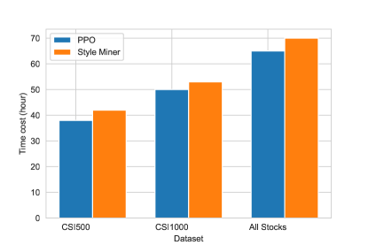
Figure 5: Cost time comparison.

As shown in Figure 5, the more stocks in the dataset, the more time cost. But the differences between PPO and StyleMiner are always small.

C.3 Factor Visualization

In order to display the style factors more intuitively, we visualized first five factors values on a random stock generated by Style Miner and PPO according to the original data for the test set. The Figure 6 shows that Style Miner has smoother output all the time.

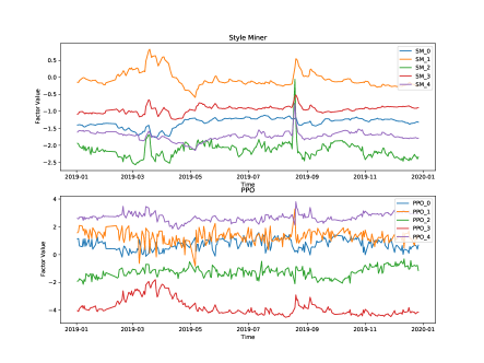
Figure 6: Factor value.

References

- Altman [1999] Eitan Altman. Constrained Markov decision processes: stochastic modeling. Routledge, 1999.
- Bahdanau et al. [2015] Dzmitry Bahdanau, Kyunghyun Cho, and Yoshua Bengio. Neural machine translation by jointly learning to align and translate. In Yoshua Bengio and Yann LeCun, editors, 3rd International Conference on Learning Representations, ICLR 2015, San Diego, CA, USA, May 7-9, 2015, Conference Track Proceedings, 2015.
- Bindoff et al. [2013] Nathaniel L Bindoff, Peter A Stott, Krishna Mirle AchutaRao, Myles R Allen, Nathan Gillett, David Gutzler, Kabumbwe Hansingo, Gabriele Hegerl, Yongyun Hu, Suman Jain, et al. Detection and attribution of climate change: from global to regional. 2013.
- Cho et al. [2014] Kyunghyun Cho, Bart van Merriënboer, Caglar Gulcehre, Dzmitry Bahdanau, Fethi Bougares, Holger Schwenk, and Yoshua Bengio. Learning phrase representations using RNN encoder–decoder for statistical machine translation. In Proceedings of the 2014 Conference on Empirical Methods in Natural Language Processing (EMNLP), pages 1724–1734, Doha, Qatar, 2014. Association for Computational Linguistics.
- Duan et al. [2022] Yitong Duan, Lei Wang, Qizhong Zhang, and Jian Li. Factorvae: A probabilistic dynamic factor model based on variational autoencoder for predicting cross-sectional stock returns. 2022.
- Fama and French [1993] Eugene F Fama and Kenneth R French. Common risk factors in the returns on stocks and bonds. Journal of financial economics, 33(1):3–56, 1993.
- Fama and French [2020] Eugene F Fama and Kenneth R French. Comparing cross-section and time-series factor models. The Review of Financial Studies, 33(5):1891–1926, 2020.
- Fama and MacBeth [1973] Eugene F Fama and James D MacBeth. Risk, return, and equilibrium: Empirical tests. Journal of political economy, 81(3):607–636, 1973.
- Fujimoto et al. [2018] Scott Fujimoto, Herke van Hoof, and David Meger. Addressing function approximation error in actor-critic methods. In Jennifer G. Dy and Andreas Krause, editors, Proceedings of the 35th International Conference on Machine Learning, ICML 2018, Stockholmsmässan, Stockholm, Sweden, July 10-15, 2018, volume 80 of Proceedings of Machine Learning Research, pages 1582–1591. PMLR, 2018.
- Golub and Reinsch [1971] Gene H Golub and Christian Reinsch. Singular value decomposition and least squares solutions. In Linear algebra, pages 134–151. Springer, 1971.
- Gu et al. [2021] Shihao Gu, Bryan Kelly, and Dacheng Xiu. Autoencoder asset pricing models. Journal of Econometrics, 222(1):429–450, 2021.
- Guy. [1975] Rosenberg James Guy. The prediction of systematic risk. Research Program in Finance Working Papers, 1975.
- Hegerl and Zwiers [2011] Gabriele Hegerl and Francis Zwiers. Use of models in detection and attribution of climate change. Wiley interdisciplinary reviews: climate change, 2(4):570–591, 2011.
- Ilmanen [2012] Antti Ilmanen. Understanding expected returns. In CFA Institute Conference Proceedings Quarterly, 2012.
- Kelly et al. [2019] Bryan T Kelly, Seth Pruitt, and Yinan Su. Characteristics are covariances: A unified model of risk and return. Journal of Financial Economics, 134(3):501–524, 2019.
- Lillicrap et al. [2016] Timothy P. Lillicrap, Jonathan J. Hunt, Alexander Pritzel, Nicolas Heess, Tom Erez, Yuval Tassa, David Silver, and Daan Wierstra. Continuous control with deep reinforcement learning. In Yoshua Bengio and Yann LeCun, editors, 4th International Conference on Learning Representations, ICLR 2016, San Juan, Puerto Rico, May 2-4, 2016, Conference Track Proceedings, 2016.
- Lin et al. [2021] Hengxu Lin, Dong Zhou, Weiqing Liu, and Jiang Bian. Deep risk model: a deep learning solution for mining latent risk factors to improve covariance matrix estimation. In Proceedings of the Second ACM International Conference on AI in Finance, pages 1–8, 2021.
- Menchero et al. [2011] Jose Menchero, D Orr, and Jun Wang. The barra us equity model (use4), methodology notes. English, MSCI May, 2011.
- Pan et al. [2022] Feiyang Pan, Tongzhe Zhang, Ling Luo, Jia He, and Shuoling Liu. Learn continuously, act discretely: Hybrid action-space reinforcement learning for optimal execution, 2022.
- Ping Tian and others [2013] Dong Ping Tian et al. A review on image feature extraction and representation techniques. International Journal of Multimedia and Ubiquitous Engineering, 8(4):385–396, 2013.
- Schulman et al. [2017] John Schulman, Filip Wolski, Prafulla Dhariwal, Alec Radford, and Oleg Klimov. Proximal policy optimization algorithms. arXiv preprint arXiv:1707.06347, 2017.
- Sharpe [1964] William F Sharpe. Capital asset prices: A theory of market equilibrium under conditions of risk. The journal of finance, 19(3):425–442, 1964.
- Sheikh [1996] Aamir Sheikh. Barra’s risk models. Barra Research Insights, pages 1–24, 1996.
- Velickovic et al. [2018] Petar Velickovic, Guillem Cucurull, Arantxa Casanova, Adriana Romero, Pietro Liò, and Yoshua Bengio. Graph attention networks. In 6th International Conference on Learning Representations, ICLR 2018, Vancouver, BC, Canada, April 30 - May 3, 2018, Conference Track Proceedings. OpenReview.net, 2018.
- Wold et al. [1987] Svante Wold, Kim Esbensen, and Paul Geladi. Principal component analysis. Chemometrics and intelligent laboratory systems, 2(1-3):37–52, 1987.