Data Augmentation For Label Enhancement

Abstract

Label distribution (LD) uses the description degree to describe instances, which provides more fine-grained supervision information when learning with label ambiguity. Nevertheless, LD is unavailable in many real-world applications. To obtain LD, label enhancement (LE) has emerged to recover LD from logical label. Existing LE approach have the following problems: (i) They use logical label to train mappings to LD, but the supervision information is too loose, which can lead to inaccurate model prediction; (ii) They ignore feature redundancy and use the collected features directly. To solve (i), we use the topology of the feature space to generate more accurate label-confidence. To solve (ii), we proposed a novel supervised LE dimensionality reduction approach, which projects the original data into a lower dimensional feature space. Combining the above two, we obtain the augmented data for LE. Further, we proposed a novel nonlinear LE model based on the label-confidence and reduced features. Extensive experiments on 12 real-world datasets are conducted and the results show that our method consistently outperforms the other five comparing approaches.

1 Introduction

The process of learning is to build a mapping from instances to labels. The learning process of one sample corresponding to one label is not adequate for many tasks in the real world, based on which ambiguous learning is proposed, i.e. one instance corresponding to multiple class labels. The above learning process, also commonly referred to as multi-label learning (MLL). MLL uses strict logical label to divide the label into relevant and irrelevant label, however, the relevance or irrelevance of labels to instances is not absolute in real-world tasks. When multiple labels are associated with an instance, the relative importance between them may be differentXu et al. (2020). As an example, when ”mountain” and ”tree” are relevant to the two images in Fig. 1, it is clear that they differ in importance (in image(a), ”tree” are more significant than ”mountain”, while in image(b) the opposite is true). At the same time, the importance of irrelevant labels may also vary, as shown in Fig. 1, where ”sun” and ”lake” in image(a) are less irrelevant than in image(b). Therefore, directly labeling each relevant and irrelevant label using a logical label would ignore the relative importance of the label.

To solve this problem, Geng proposed a new learning paradigm called label distribution learning (LDL) Geng (2016). Different from MLL, LDL assumes that an instance is annotated by an LD over all possible labels instead of a binary label vector. For example, give an instance $\mathbf{x}$, $d_{\mathbf{x}}^{y}\in[0,1]$ denotes the description degree of the label $y$ to the instance $\mathbf{x}$, and $\sum_{y}d_{\mathbf{x}}^{y}=1$. LDL allows a better representation of the relativity between labels, thus it has many real-world applications, such as pre-release prediction of crowd opinion on movies Geng and Hou (2015), video parsing Geng and Ling (2017), historical context-based style classification of painting images Yang et al. (2018), and children’s empathy ability analysis Chen et al. (2021). However, LDs usually require extensive expert annotation, and therefore collecting LDs is very expensive. This led to the creation of an algorithm to recover LDs from training data in bulk, the process called label enhancementXu et al. (2019a). In recent years, LE has been successfully applied to multi-label learningZhao et al. (2022), label distribution learningGao et al. (2020), partial label learningXu et al. (2019b), etc.

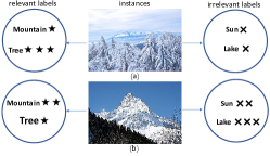
Figure 1: An example of the relative importance between relevant (irrelevant) labels between different instances

Motivation Existing LE algorithms used the logical label directly to train a mapping to the LD and then normalize the predicted distribution. In classification tasks, logical label can provide accurate supervisory information, but when the goal is to recover an LD, it provides poor information. In addition, the collected features are usually containing redundant information, the existing LE algorithm directly uses the collected features to train the model, which will lead to poor generalization of the model.

To deal with these challenges, we proposed a data augmented LE approach, LCdr. Specifically, logical label provide little information, we utilised the local consistency of the instances to learn a label-confidence that can provide more information. Next, for the first time we proposed a supervised dimensionality reduction approach in LE, which attemptes to projects the high-dimensional feature matrix containing redundant information into a low-dimensional space. We called this process above data-augmentation (DA). Finally, we proposed a non-linear LE model based on augmented data. Extensive experiments on real-world datasets demonstrate the superiority of the proposed approach and the effectiveness of augmented data.
Our contribution is summarised below:

• For the first time, we use the label-confidence generated by the local consistency of instances to guide learning instead of logical label. This accurate supervisory information seems to improve the performance in LE.

• For the first time, we used the dimensionality reduction technology in label enhancement, and proved that DR can improve the generalizability of LE model.

• Our approach achieves superior performance against five existing LE algorithms on twelve real-world datasets, and the proposed approach seems to cooperate with any LE algorithm.

2 Related Work

2.1 Label Distribution Learning

Label Distribution Learning (LDL) Geng (2016) as a new learning paradigm, using LD to labeling instances and learns a mappings from instances to LD. Thus, in learning with label ambiguity task, the LD describes the supervised information at a finer granularity than the logical label. LDL has been successfully applied to many real applications, such as estimation of the age of the speaker Si et al. (2022), predictions of the composition of Martian craters Morrison et al. (2018), facial depression recognition Zhou et al. (2022), joint acne image grading Wu et al. (2019), depression detection de Melo et al. (2019), indoor crowd counting Ling and Geng (2019), and head pose estimation Geng et al. (2020).

2.2 Label Enhancement

The acquisition of LD often requires expert annotation, so the collection of LD is difficult. To obtain LD more easily, an algorithm for recovering the LD from the logical label is proposed, and this algorithm is named Label EnhancementXu et al. (2019a). In this section, we briefly review the researches in LE. Label propagation techniques for generating label distributions in LP Zhang et al. (2021) by propagating label importance information. ML Hou et al. (2016) generates label distributions through the idea of manifold learning by means of the technique of locality embedding. LEMLL Shao et al. (2018) assumed that the label distribution space should share a similar local topology in the feature space, and a locally linear embedding technique is used to implement LE. GLLE Xu et al. (2018) constructed a local similarity matrix to preserve the structure of the feature space, and use the local similarity matrix to transform logical labels into label distributions. LESC Zheng et al. (2020) proposed a low-rank representation of LE by capturing the global relationships of samples and predicting implicit label correlations. LEVI Xu et al. (2022) used variational inference techniques applied to LE to introduce a generative model of the label distributions while giving a variational lower bound on the recovered label distributions.

Although a number of LE algorithms have been proposed, there are no LE algorithms designed from a data representation perspective. The label space can be thought of as a low-dimensional representation of the feature space, where the collected feature and label are recorded as a set of data. A better representation of the data will undoubtedly improve the performance for LE. In the next section, a novel data augmentation (DA) approach is proposed for LE.

3 Data Augmentation for Label Enhancement

Problem Setup The goal of LE is to recover a label distribution matrix $\mathbf{D}=\left[\mathbf{d}_{1},\mathbf{d}_{2},\ldots,\mathbf{d}_{n}\right]\in\mathbbm{R}^{q\times n}$ from the training set $\mathcal{T}=\mathbf{(X,L)}$. We denote $Y=\left\{y_{1},y_{2},\ldots,y_{q}\right\}$ as the label space with q class labels, $\mathbf{d}_{i}=\left[d_{\mathbf{x}_{i}}^{y_{1}},d_{\mathbf{x}_{i}}^{y_{2}},\ldots,d_{\mathbf{x}_{i}}^{y_{q}}\right]\in\mathbf{D}$ as the label distribution vector to the $i$th sample $\mathbf{x}_{i}$, and $d_{\mathbf{x}_{i}}^{y}$ indicates the importance degree of label $y$ to $\mathbf{x}_{i}$. We denote $\mathbf{X}=\left[\mathbf{x}_{1},\mathbf{x}_{2},\ldots,\mathbf{x}_{n}\right]\in\mathbbm{R}^{d\times n}$ as feature matrix and $\mathbf{L}=\left[\mathbf{l}_{1},\mathbf{l}_{2},\ldots,\mathbf{l}_{n}\right]\in\mathbbm{R}^{q\times n}$ as the corresponding logical label matrix, where $\mathbf{{l}}_{i}=\left(l_{{\mathbf{x}}_{i}}^{y_{1}},l_{{\mathbf{x}}_{i}}^{y_{2}},\ldots,l_{{\mathbf{x}}_{i}}^{y_{q}}\right)^{\top}\in\mathbf{L}$ is the the logical label vector. We denote $n$ and $d$ as the number of training examples and the dimension of features.
Main Idea Logical label ensures that each instance is correctly classified with a large margin. When the goal of learning is to predict the LD of an instance, we need a more compact label to supervise training. In addition, LE using the collected features directly, without considering the issue of feature redundancy, can reduced generalization ability of algorithms. To solve the above problem, first we use the topology of the feature space to learn a more compact label-confidence, and then we use the LC to supervise the dimensionality reduction of the feature space. To verify whether the augmented data can learn a reasonable LE model, we proposed a augmented data based non-linear LE approach.

3.1 Generating Lable-Confidence Utilizing Local Consistency of Instances

Given an training data set $\mathcal{T}$, we aim to generate a normalized real-valued label-confidence (LC) matrix $\mathbf{F}=\left[\mathbf{f}_{1},\mathbf{f}_{2},\ldots,\mathbf{f}_{n}\right]^{\top}\in[0,1]^{n\times q}$. Where ${\mathbf{f}_{i}=\left[f_{i1},f_{i2},\ldots,f_{iq}\right]^{\top}}$ represents the LC vector, and $f_{il}$ represents the probability of the $y_{l}$ being the ground-turth label of $\mathbf{x}_{i}$. The label-confidence vector $\mathbf{f}_{i}$ satisfies the following constraints: (i) $\mathbf{x}_{i}(1\leq i\leq n)$ with $f_{il}\in[0,1]$, (ii) $\sum_{l=1}^{q}f_{il}=1$. Correspondingly, The LC matrix is initialized as:

$$\begin{gathered}\forall 1\leq i\leq n.\left\{\begin{array}[]{lll}f_{il}=1&\text{ if }&l_{il}=1\\ f_{il}=0&\text{ if }&l_{il}=0.\end{array}\right.\end{gathered}$$ (1)

Here, we use the local consistency of the feature space to estimate the LC. For multi-label learning, this method has been proven to be effective in estimating the underlying ground-truth label. Give a fully connected graph $\mathcal{G}=(\mathcal{V},\mathcal{E},\mathbf{W})$, the weight matrix $\mathbf{{W}}=\left[w_{ij}\right]_{n\times n}$ over the LE training example is defined as: $w_{ij}=\exp\left(-\left\|\mathbf{x}_{i}-\mathbf{x}_{j}\right\|_{2}^{2}/\sigma^{2}\right)$ if $\mathbf{x}_{j}\in\mathcal{N}\left(\mathbf{x}_{i}\right)$, otherwise $w_{ij}=0$, which $\sigma$ is the hyper-parameter. To ensure that our weight structure is symmetrical, we set $\mathbf{W}=\mathbf{W}+\mathbf{W}^{\top}$. After obtaining the local weight structure, we can obtain the label-confidence matrix by solving the following problem:

$$\begin{gathered}\min_{\mathbf{F}}\sum_{i=1}^{n}\sum_{j=1}^{n}w_{ij}\left\|\frac{\mathbf{f}_{i}}{\sqrt{d_{ii}}}-\frac{\mathbf{f}_{j}}{\sqrt{d_{jj}}}\right\|_{2}^{2}\\ \text{ s.t. }\sum_{l=1}^{q}f_{il}=1,\quad 1\leq i\leq n\\ f_{il}\geq 0\left(\forall l_{il}=1\right),f_{il}=0\left(\forall l_{il}=0\right),\end{gathered}$$ (2)

where $d_{ii}=\sum_{j=1}^{n}w_{ij}$ is the degre of $\mathbf{x}_{i}$ in the graph. The first term in Eq .2 enforces a degree of similarity between the label confidece of nearby points. The first constraint represents the normalized property of the label-confidence vector. The second constraint represents the label-confidence is non-negative if it logical label is 1, and the label-confidence is zero if it Logical label is 0. The optimization problem in Eq. 2 turns out to be:

$$\begin{gathered}\min_{\widetilde{\mathbf{f}}}\frac{1}{2}\widetilde{\mathbf{f}}^{\top}\mathbf{H}\widetilde{\mathbf{f}}\\ \text{ s.t. }\mathbf{F}\mathbf{1}_{q}=\mathbf{1}_{n},\mathbf{0}_{q\times n}\leq\mathbf{F}\leq\mathbf{Y},\end{gathered}$$ (3)

where $\widetilde{\mathbf{f}}=\operatorname{vec}(\mathbf{F})$, $\operatorname{vec}(\cdot)$ is the vectorization operator and $\mathbf{Q}\in\mathbb{R}^{nq\times nq}$ is defined as follows:

$$\begin{gathered}\mathbf{Q}=\left[\begin{array}[]{cccc}\mathbf{T}&\mathbf{0}_{n\times n}&\cdots&\mathbf{0}_{n\times n}\\ \mathbf{0}_{n\times n}&\mathbf{T}&\cdots&\mathbf{0}_{n\times n}\\ \vdots&\vdots&\ddots&\vdots\\ \mathbf{0}_{n\times n}&\mathbf{0}_{n\times n}&\cdots&\mathbf{T}\end{array}\right],\end{gathered}$$ (4)

where $\mathbf{T}\in\mathbb{R}^{n\times n}$ is a square matrix defined as $\mathbf{T}=4\left(\mathbf{I}_{q\times q}-\mathbf{J}^{-\frac{1}{2}}\mathbf{W}\mathbf{J}^{-\frac{1}{2}}\right)$, where $\mathbf{J}$ is a diagonal matrix with its diagonal element defined as $d_{ii}=\sum_{j=1}^{n}w_{ij}$. Eq. 3 can be solved efficiently by off-the-shelf QP tools.

By solving problem 2, we obtain a augmented LC matrix $\mathbf{F}$, and we converted the training samples from $\mathcal{T}$ to $\widetilde{T}$, where $\widetilde{T}=\left\{\left(x_{1},\boldsymbol{f}_{1}\right),\ldots,\left(x_{n},\boldsymbol{f}_{n}\right)\right\}$. Based on the LC matrix, we introduce a supervised dimensionality reduction (DR) approach in the next section.

3.2 Supervised Dimensionality Reduction for LE

To remove redundant features, we proposed a supervised dimensionality reduction approach with maximum dependency between the feature information and the label space. It is not feasible to use MLL supervised DR method directly for label enhancement, because even if two instances are different, their corresponding binary labels may be same, and direct use of MLL DR method may loss of useful feature information. Base on this, we proposed a LC-based DR approach for LE.

Specifically, we consider a linear DR matrix $\mathbf{P}$, which can projection of feature matrix $\mathbf{X}$ into a lower dimensional feature space, i.e. $\mathbf{P}^{\top}\mathbf{X}=\widetilde{\mathbf{X}}\in\mathbb{R}^{d^{\prime}\times n}(d^{\prime}\ll d)$. First, we introduce the kernel matrix of input space $\mathbf{X}$, which is defined by $\mathbf{K}=\left[k_{ij}\right]_{n\times n}$, where $k_{ij}$ is defined as: $k_{ij}=k\left(\mathbf{x}_{i},\mathbf{x}_{j}\right)=\left\langle\mathbf{P}^{\top}\mathbf{x}_{i},\mathbf{P}^{\top}\mathbf{x}_{j}\right\rangle$, next, locate the kernel matrix of the label-confidence as $\mathbf{\widetilde{F}}=[\widetilde{f}_{ij}]_{n\times n}$, where $\widetilde{f}_{ij}$ is defined as: $\widetilde{f}_{ij}=l\left(\mathbf{f}_{i},\mathbf{f}_{j}\right)=\left\langle\mathbf{f}_{i},\mathbf{f}_{j}\right\rangle$.

Then we attempt to maximize the dependence between the projected feature and the label-confidence. Here we use Hilbert-Schmidt Independence Criterion (HSIC) Gretton et al. (2005) Zhang and Zhou (2010) Bao et al. (2021), which is an effective dependency measurement method. HSIC is defined as:

$$\begin{gathered}\text{HSIC}(\mathcal{F},\mathcal{U},\widetilde{T})=(n-1)^{-2}\operatorname{tr}(\mathbf{HKH\mathbf{\widetilde{F}}}),\end{gathered}bi$$ (5)

where $\mathcal{F},\mathcal{U}$ is the reproducing kernel Hilbert space mapped from $\mathbf{X}$ and $\mathbf{F}$ respectively, tr($\cdot$) is the trace norm and $\mathbf{H}=\mathbf{I}-\frac{1}{m}\mathbf{e}\mathbf{e}^{\top}$, where $\mathbf{e}$ is an all-one column vector. However, there is still redundant information in the projected low-dimensional features. To maximize the retention of useful features, We constrain the projection vectors to be linearly uncorrelated with each other, i.e. $\mathbf{p}_{i}^{\top}\mathbf{X}\mathbf{X}^{\top}\mathbf{p}_{j}=\delta_{ij}$, where $\delta_{ij}$=1 if i=j and $\delta_{ij}$=0 otherwise. Finally, we set the bases of the projection to be orthonormal, which is denoted as $\mathbf{p}_{i}^{\top}\mathbf{p}_{j}=\delta_{ij}$. Substituting $\mathbf{K}=\mathbf{X}^{\top}\mathbf{P}\mathbf{P}^{\top}\mathbf{X}$ and the joint constraint into Eq. 5 and dropping the normalization term, we obtain the objective function as follows:

$$\max_{\mathbf{P}}\operatorname{tr}\left(\mathbf{HX}^{\top}\mathbf{P}\mathbf{P}^{\top}\mathbf{XH\widetilde{F}}\right)$$ (6)

$$\text{ s.t. }\alpha\mathbf{p}_{i}^{\top}\mathbf{X}\mathbf{X}^{\top}\mathbf{p}_{j}+(1-\alpha)\mathbf{p}_{i}^{\top}\mathbf{p}_{j}=\delta_{ij},$$

where $\alpha$ is trade-off parameter. The solution of Eq. 6 can be obtained easily by the Lagrangian method. Specifically, we set the derivative of the Lagrangian function of Eq. 6 to 0, and then $\mathbf{P}$ can be obtained by find the eigenvectors ($\mathbf{V}$) of $\mathbf{XH\widetilde{F}H}\mathbf{X}^{\top}$ and $\alpha\mathbf{XX}^{\top}+(1-\alpha)\mathbf{I}$, here we use the Matlab function $\mathbf{V}=$eig($\cdot$,$\cdot$). Then, we sort the matrix of eigenvalues in descending order ( $\mathbf{P}^{\prime}$=sort($\mathbf{V}$, ’descend’)), and select the largest $d^{\prime}$ eigenvalues as the DR matrix, i.e.

$$\mathbf{P}=\mathbf{P}^{\prime}(:,1:d^{\prime}).$$ (7)

we can control the dimensionality of the projected feature space by setting the different threshold parameter $d^{\prime}$. By solving for the problem 6, we obtain a low-dimensional feature matrix $\mathbf{\widetilde{X}}$, and combined with the previous section, we obtain the $\mathbf{augmented}$ $\mathbf{data}$, i.e. $\mathbbm{T}^{\prime}=\left\{\left(\mathbf{\widetilde{x}}_{i},\mathbf{f}_{i}\right)\mid 1\leqslant i\leqslant n\right\}$, where $\mathbf{\widetilde{x}}_{i}=\mathbf{P}^{\top}\mathbf{x}_{i}$. In the next section, based on the augmented data, we proposed a label-confidence dimensionality reduction (LCdr) approach to recover label distribution.

3.3 Non-linear LE Methods based on Augmented Data

To verify the effectiveness of the data augmentation, we proposed a new LE model named LCdr, which is defined as:

$$\mathcal{L}_{le}=\sum_{i=1}^{n}\left\|\mathbf{f}_{i}-\left[\sigma\left(\mathbf{w}_{i}\widetilde{\mathbf{x}}_{i}\right)\right]_{\text{Softmax }}\right\|_{2}^{2}+\sum_{i=1}^{n}\beta\|\mathbf{w}_{i}\|_{2}^{2},$$ (8)

where $\mathbf{w}_{i}\in\mathbf{W}^{q\times d^{\prime}}$ is weighting matrix, $\beta$ is a trade-off parameter, $\sigma(\cdot)$ is the activation function, here, we use the Relu-function, and Softmax$(\cdot)$ is the normalization function. The Relu-function ensures that the mapping between low-dimensional features and LC is non-linear, which allows our model to learn more complex relationships between the data. The Softmax$(\cdot)$ fuction ensured the learned distribution is non-zero and normalised. The Second term of loss fuction 8 prevents our model from overfitting.

Implementation Details We use the stochastic gradient descent (SGD) algorithm in PyTorch to solve Eq. 8, and We set $\beta=0.1$, the learning rate to 0.01, the momentum to 0.9 and the weight-decay to 5e-4. The learning process continues until convergence or reaches predefined maximum iterations.

The model iterates until it converges, and finally, we directly predict the LD of the training instances.

Augmented data can cooperate with many existing LE approach such as GLLE Xu et al. (2019a), LESC Tang et al. (2020), LEMLL Shao et al. (2018), LP Zhang et al. (2021), ML2 Hou et al. (2016). Algorithm 1 summarizes the pseudo-code of the proposed approach.

Algorithm 1 The pseudo-code of the proposed approach

Input:
$\mathcal{T}$: LE training set $\left\{\left(\mathbf{x_{i}},\mathbf{l_{i}}\right)\mid 1\leq i\leq n\right\}$
$k$: the number of neighbors for weighted graph construction
$d^{\prime}$: the threshold parameter in Eq. 7
$\alpha$: the trade-off parameter in Eq. 6
$\mathcal{F}$: the proposed approach, which is defined as Eq. 8;
$\mathcal{R}$: any label enhancement algorithm
Output:
$\mathbf{D}_{1}$: the predicted LD by $\mathcal{F}$,
$\mathbf{D}_{2}$: the predicted LD by $\mathcal{R}$;
Process:

1: Set the fully connected graph $\mathcal{G}=(\mathcal{V},\mathcal{E},\mathbf{W})$, and calculate the weight matrix $\mathbf{W}$;

2: Initialize the $q$×$n$ label-confidence matrix $\mathbf{F}$ based on Eq. 1;

3: repeat

4:    Update $\mathbf{F}$ by solving Eq.2;

5: until convergence

6: return  $\mathbf{F}$;

7: repeat

8:    Calculate kernel matrix $\mathbf{\widetilde{F}}=\left\langle\mathbf{f}_{i},\mathbf{f}_{j}\right\rangle$ and $\mathbf{H}=\mathbf{I}-\frac{1}{m}\boldsymbol{e}\boldsymbol{e}^{\top}$;

9:    Solve the problem 6, and then get the projection matrix $\mathbf{P}$;

10: until convergence

11: return  the lower-dimensional features space : $\widetilde{\mathbf{X}}=\mathbf{P}^{\top}\mathbf{X}$;

12: Transformed the augmented LE training set $\mathbbm{T}^{\prime}=(\widetilde{\mathbf{X}},\mathbf{F})$;

13: return  $\mathbf{D}_{1}=\mathcal{F}(\mathbbm{T}^{\prime})$;

14: return  $\mathbf{D}_{2}=\mathcal{R}(\mathbbm{T}^{\prime})$;  

4 Experiments

Datasets and evaluation measure: We validate the effectiveness of LCdr on 12 real data sets, with the specific details of the data shown in Table2. Where the first 10 real-world datasets are collected from the records of 10 biological experiments on the budding yeast genesEisen et al. (1998), the last datasets Flickr-LDL and Twitter-LDLYang et al. (2017) are are two two facial expression datasets. More details of them can be found in Geng (2016). Where the logical labels in the datasets are obtained by LD degradation, here we use the same strategy as GLLEXu et al. (2018), which can be roughly described as setting a threshold, where logical labels with a degree of description more than the threshold are 1 and the rest are 0. Following Geng Geng (2016), seven metrics are used to evaluate the ability to recover, i.e., Chebyshev$\downarrow$, Clark$\downarrow$, Kullback-Leibler(KL)$\downarrow$, Canberra$\downarrow$, S$\phi$rensen$\downarrow$ and Cosine$\uparrow$, ↑ (resp. ↓) means the larger (resp. smaller), the better, and the seven measures are summarized in Table 2.

Measure	Formula
Chebyshev $\downarrow$	$\operatorname{Dis}_{1}(\boldsymbol{d},\hat{\boldsymbol{d}})=\max_{j}\left|d_{j}-\hat{d}_{j}\right|$
Clark	$\operatorname{Dis}_{2}(\boldsymbol{d},\hat{\boldsymbol{d}})=\sqrt{\sum_{j=1}^{c}\frac{\left(d_{j}-\hat{d}_{j}\right)^{2}}{\left(d_{j}+\hat{d}_{j}\right)^{2}}}$
Canberra $\downarrow$	$\operatorname{Dis}_{3}(\boldsymbol{d},\hat{\boldsymbol{d}})=\sum_{j=1}^{c}\frac{\left|d_{j}-\hat{d}_{j}\right|}{d_{j}+\hat{d}_{j}}$
Kullback-Leibler$\downarrow$	$\operatorname{Dis}_{4}(\boldsymbol{d},\hat{\boldsymbol{d}})=\sum_{j=1}^{c}d_{j}\ln\frac{d_{j}}{\hat{d}_{j}}$
cosine	$\operatorname{Sim}_{1}(\boldsymbol{d},\hat{\boldsymbol{d}})=\frac{\sum_{j=1}^{c}d_{j}\hat{d}_{j}}{\sqrt{\sum_{j=1}^{c}d_{j}^{2}}\sqrt{\sum_{j=1}^{c}\hat{d}_{j}^{2}}}$
intersection $\uparrow$	$\operatorname{Sim}_{2}(\boldsymbol{d},\hat{\boldsymbol{d}})=\sum_{j=1}^{c}\min\left(d_{j},\hat{d}_{j}\right)$

Table 1: The distribution distance/similarity measures

ID	Dataset	Examples	Features	Labels
1	Yeast-dtt (dtt)	2465	24	4
2	Yeast-spo (spo)	2465	24	6
3	Yeast-spo5 (spo5)	2465	24	3
4	Yeast-diau (diau)	2465	24	7
5	Yeast-cold (cold)	2465	24	4
6	Yeast-spoem(spoem)	2465	24	2
7	Yeast-cdc (cdc)	2465	24	15
8	Yeast-alpha (alpha)	2465	24	18
9	Yeast-elu (elu)	2465	24	14
10	Yeast-heat (heat)	2465	24	5
11	Flickr-LDL (Flickr)	11150	200	8
12	Twitter-LDL(Twitter)	10045	200	8

Table 2: Details of the datasets.

Implementation Details: First we verify whether the proposed method can recover better LD from logical label than other LE algorithms. Next, we verify whether extending the data augmentation strategy to other LE algorithms enables it to learn a reasonable LE model. Finally, we checked to ensure that the recovered LD could be trained to produce a more reasonable LDL model.

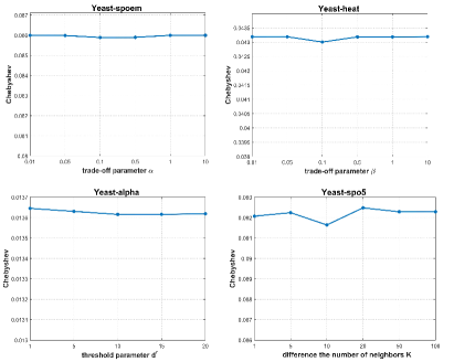
Figure 2: Performance of the proposed method as the parameter $\alpha$, $\beta$, $d^{\prime}$ and $K$ vary on different data sets.

chebyshev $\downarrow$
	spoem	alpha	spo5	cdc	cold	diau	dtt	elu	heat	spo	flickr	twitter
ours	0.0859	0.0136	0.0916	0.0166	0.0535	0.0413	0.0366	0.0165	0.0432	0.0596	0.0614	0.0730
LP	0.1286	0.0243	0.1040	0.0297	0.1002	0.0625	0.1017	0.0309	0.0699	0.0698	0.0661	0.0753
ML2	0.3024	0.6264	0.2670	0.5394	0.2795	0.3823	0.2766	0.5208	0.3097	0.2835	0.1093	0.2467
GLLE	0.0880	0.0190	0.0978	0.0216	0.0638	0.0515	0.0505	0.0223	0.0476	0.0599	0.0640	0.0782
LESC	0.0892	0.0183	0.1013	0.0220	0.0631	0.0547	0.0520	0.0233	0.0504	0.0640	0.0837	0.0792
LEMLL	0.1126	0.0397	0.1134	0.0442	0.1241	0.1045	0.1154	0.0479	0.0826	0.0777	0.0647	0.0815
clark $\downarrow$
	spoem	alpha	spo5	cdc	cold	diau	dtt	elu	heat	spo	flickr	twitter
ours	0.1276	0.2148	0.1847	0.2190	0.1452	0.2206	0.0996	0.2042	0.1866	0.2536	0.2417	0.2649
LP	0.2062	0.8226	0.2453	0.7369	0.3524	0.4669	0.3799	0.7119	0.4321	0.3971	0.4693	0.3881
ML2	0.6195	3.4836	0.7556	2.9377	1.0435	1.6434	1.0491	2.7752	1.3994	1.3311	0.6439	1.4296
GLLE	0.1313	0.3261	0.1942	0.3003	0.1704	0.2916	0.1380	0.2839	0.2064	0.2585	0.3058	0.3071
LESC	0.1327	0.3085	0.2022	0.3020	0.1700	0.2934	0.1407	0.2938	0.2179	0.2744	0.4154	0.3174
LEMLL	0.1842	0.7693	0.2441	0.6702	0.3506	0.5848	0.3479	0.6604	0.3964	0.3724	0.3017	0.3058
canberra $\downarrow$
	spoem	alpha	spo5	cdc	cold	diau	dtt	elu	heat	spo	flickr	twitter
ours	0.1776	0.6984	0.2836	0.6545	0.2504	0.4730	0.1709	0.6010	0.3721	0.5233	0.5587	0.6135
LP	0.2803	3.3451	0.3617	2.7223	0.6619	1.1169	0.7267	2.5437	0.9872	0.8897	1.2230	1.0005
ML2	0.7892	14.1515	1.0781	10.7003	1.8913	3.9351	1.9135	9.7282	3.1178	2.9511	1.6257	3.8012
GLLE	0.1825	1.0962	0.3012	0.9370	0.2957	0.6631	0.2401	0.8675	0.4170	0.5353	0.7208	0.7058
LESC	0.1846	1.0455	0.3123	0.9352	0.2938	0.6443	0.2441	0.8908	0.4412	0.5653	0.9618	0.7219
LEMLL	0.2491	2.8064	0.3688	2.2412	0.6195	1.3242	0.6225	2.1466	0.8450	0.7861	0.7360	0.7208
K-L $\downarrow$
	spoem	alpha	spo5	cdc	cold	diau	dtt	elu	heat	spo	flickr	twitter
ours	0.0274	0.0058	0.0317	0.0076	0.0135	0.0166	0.0066	0.0066	0.0137	0.0272	0.0182	0.0228
LP	0.0449	0.0668	0.0363	0.0645	0.0566	0.0533	0.0651	0.0640	0.0558	0.0482	0.0530	0.0436
ML2	0.2410	1.8433	0.2447	1.4508	0.3896	0.7066	0.4006	1.3624	0.5468	0.4789	0.0895	0.4202
GLLE	0.0276	0.0123	0.0328	0.0130	0.0177	0.0259	0.0119	0.0124	0.0164	0.0274	0.0281	0.0301
LESC	0.0284	0.0117	0.0364	0.0137	0.0180	0.0283	0.0128	0.0136	0.0184	0.0307	0.0523	0.0318
LEMLL	0.0406	0.0629	0.0407	0.0582	0.0636	0.0900	0.0614	0.0610	0.0519	0.0466	0.0234	0.0281
cosine $\uparrow$
	spoem	alpha	spo5	cdc	cold	diau	dtt	elu	heat	spo	flickr	twitter
ours	0.9783	0.9944	0.9738	0.9930	0.9875	0.9856	0.9940	0.9938	0.9873	0.9753	0.9778	0.9711
LP	0.9664	0.9445	0.9740	0.9465	0.9546	0.9578	0.9470	0.9471	0.9547	0.9611	0.9554	0.9619
ML2	0.8741	0.4002	0.8782	0.4791	0.8044	0.6917	0.7916	0.4993	0.7460	0.7773	0.9304	0.7982
GLLE	0.9774	0.9880	0.9713	0.9877	0.9832	0.9760	0.9888	0.9879	0.9847	0.9753	0.9723	0.9634
LESC	0.9769	0.9886	0.9687	0.9870	0.9831	0.9740	0.9879	0.9868	0.9827	0.9720	0.9452	0.9617
LEMLL	0.9705	0.9451	0.9671	0.9491	0.9482	0.9274	0.9497	0.9467	0.9565	0.9619	0.9756	0.9723

Table 3: The recovery results on the real-world datasets measured by (Chebyshev$\downarrow$, Clark$\downarrow$, Canberra$\downarrow$, K-L $\downarrow$, Cosine$\uparrow$).

Comparing Methods: We compare LCdr against five LE approaches with parameter configurations suggested in respective literatures.

• GLLEXu et al. (2021): GllE recovers LD directly from the logical label using the graph Laplacian method, where the regularisation parameter $\lambda$is set to 0.01 and the number of neighbors K is set to q+ 1.

• LESCTang et al. (2020): LESC used a low-rank representation to capture the global relationship of the sample and predict the LD of the sample. The parameters $\lambda_{1}$ and $\lambda_{2}$ are selected among $\{0.0001,0.001,\ldots,10\}$.

• LEMLLShao et al. (2018): LEMLL L used the topology of the feature space to recover LD. We set the irrelevant marker to -1, the number of neighbors K is 3, instances whose distance computed is more than $\epsilon$ should be penalized as 10, and the type of kernel function is Lin.

• LPZhang et al. (2021):LP used label propagation techniques to generate LD. We also choose the parameter $\alpha$ in LP to be 0.01.

• ML2Hou et al. (2016): ML2 Used the manifold technique to generated LD. We set the number of neighbors K is set to q+ 1.

• LCdr: We set the number of neighbors K=10, the threshold parameter $d^{\prime}$=10, the trade-off parameter $\alpha$=$\beta$=0.1.

Metric	LCdr	LP	ML2	GLLE	LESC	LEMLL
chebyshev	1.00	3.92	6.00	2.25	3.08	4.75
clark	1.00	4.92	6.00	2.33	3.00	3.75
canberra	1.00	4.83	6.00	2.33	2.83	4.00
K-L	1.00	4.67	6.00	2.25	3.17	3.92
cosine	1.17	4.25	6.00	2.33	3.33	3.92

Table 4: The average ranks of six algorithms on five measures in the LD recovered experiment.

4.1 Results

4.1.1 LD Recovery Performance

For quantitative analysis, table 3 tabulates the results of the five LE algorithms on all real-world datasets, and the best performance is highlighted. Note that since each LE algorithm only runs once, there is no record of standard deviation. The average ranks of six algorithms on five measures as shown in Table 4. To analyze whether there are statistical performance gaps among comparing algorithms, Wilcoxon signed-ranks testDemsar (2006), which is a widely-accepted statistical test for comparisons of two algorithms over several datasets, is employed. Table 7 summarizes the statistical test results and the p-values for the corresponding tests are also shown in the brackets. From the above results, we have the following observations:

• Compared to the five algorithms LP, ML2, GLLE, LESC, and LEMLL, the proposed method achieves better performance in all cases (12 datasets and five metrics).

• The proposed approach achieves statistically superior performance against comparing methods in terms of the five metrics.

chebyshev $\downarrow$
Dataset	GLLE	LCdr-GLLE	ML2	LCdr-ML2	LP	LCdr-LP	LESC	LCdr-LESC	LEMLL	LCdr-LEMLL
spoem	0.1318	0.1261	0.6195	0.1366	0.2062	0.0828	0.1364	0.1281	0.1961	0.0899
alpha	0.3261	0.2375	3.4836	0.2187	0.8226	0.2116	0.3085	0.2329	0.7693	0.2129
spo5	0.1938	0.1848	0.7556	0.2283	0.2737	0.1446	0.2022	0.1912	0.2441	0.1458
cdc	0.3058	0.2751	0.6439	0.5055	0.4693	0.2411	0.4154	0.2716	0.3017	0.2551
cold	0.3071	0.3000	1.4296	0.6960	0.3881	0.2718	0.3174	0.2586	0.3058	0.2757
diau	0.3003	0.2974	2.9377	0.2191	0.7369	0.2130	0.3020	0.2559	0.6702	0.2179
dtt	0.1704	0.1434	1.0435	0.1466	0.3524	0.1096	0.1700	0.1593	0.3506	0.1349
elu	0.2916	0.2214	1.6434	0.2225	0.4669	0.2046	0.2934	0.2321	0.5848	0.2138
heat	0.1380	0.1380	1.0491	0.1016	0.3799	0.0727	0.1407	0.1320	0.3479	0.0840
spo	0.2839	0.2180	2.7752	0.2106	0.7119	0.1977	0.2938	0.2403	0.6604	0.2016
flickr	0.2064	0.1898	1.3994	0.1871	0.4321	0.1640	0.2179	0.1975	0.3964	0.1782
twitter	0.2585	0.2581	1.3311	0.2559	0.3971	0.2313	0.2744	0.2705	0.3724	0.2471
K-L $\downarrow$
Datasets	GLLE	LCdr-GLLE	ML2	LCdr-ML2	LP	LCdr-LP	LESC	LCdr-LESC	LEMLL	LCdr-LEMLL
spoem	0.0276	0.0263	0.2410	0.0371	0.0449	0.0174	0.0298	0.0274	0.0447	0.0184
alpha	0.0123	0.0069	1.8433	0.0064	0.0668	0.0062	0.0117	0.0067	0.0629	0.0062
spo5	0.0327	0.0313	0.2447	0.0519	0.0426	0.0228	0.0364	0.0332	0.0407	0.0196
cdc	0.0281	0.0232	0.0895	0.0696	0.0530	0.0180	0.0523	0.0224	0.0234	0.0200
cold	0.0301	0.0271	0.4202	0.1313	0.0436	0.0238	0.0318	0.0216	0.0281	0.0217
diau	0.0130	0.0128	1.4508	0.0082	0.0645	0.0079	0.0137	0.0100	0.0582	0.0081
dtt	0.0177	0.0132	0.3896	0.0161	0.0566	0.0109	0.0180	0.0159	0.0636	0.0144
elu	0.0259	0.0166	0.7066	0.0182	0.0533	0.0160	0.0283	0.0183	0.0900	0.0170
heat	0.0119	0.0118	0.4006	0.0091	0.0651	0.0062	0.0128	0.0115	0.0614	0.0071
spo	0.0124	0.0075	1.3624	0.0077	0.0640	0.0070	0.0136	0.0091	0.0610	0.0071
flickr	0.0164	0.0141	0.5468	0.0153	0.0558	0.0126	0.0184	0.0151	0.0519	0.0141
twitter	0.0274	0.0278	0.4789	0.0293	0.0482	0.0251	0.0307	0.0302	0.0466	0.0277

Table 5: The recovery experiments results measured by chebyshev$\downarrow$ and K-L$\downarrow$. For the LE algorithm $\mathcal{F}\in\{$ GLLE,LESC, ML2, LP, LEMLL $\}$, the performance of the $\mathcal{F}$-LCdr is compared against that of $\mathcal{F}$.

	spoem	alpha	spo5	cdc	cold	diau	dtt	elu	heat	spo	flickr	twitter
LF+LC	0.0859	0.0136	0.0916	0.0163	0.0535	0.0413	0.0366	0.0165	0.0432	0.0596	0.0614	0.0730
X+LF	0.0881	0.0137	0.0926	0.0165	0.0547	0.0421	0.0367	0.0166	0.0434	0.0605	0.0656	0.0782
LF+L	0.0874	0.0164	0.0976	0.0197	0.0517	0.0678	0.0376	0.0192	0.0460	0.0601	0.0691	0.0834
X+L	0.0886	0.0191	0.1338	0.0305	0.0834	0.0791	0.0590	0.0218	0.0593	0.0723	0.3270	0.0906

Table 6: Ablation experiments for recovery experiments measured by Chebyshev $\downarrow$. ($\mathbf{LC}$ representatives the label-confidence, $\mathbf{LF}$ representatives the lower-dim features, $\mathbf{X}$ representatives the original features, $\mathbf{L}$ representatives the logical labels.)

Method	Chebyshev$\downarrow$	Clark$\downarrow$	Canberra$\downarrow$	K-L $\downarrow$	Cosine$\uparrow$
LP	win[4.88e-04]	win[4.88e-04]	win[4.88e-04]	win[4.88e-04]	win[9.77e-04]
ML2	win[4.88e-04]	win[4.88e-04]	win[4.88e-04]	win[4.88e-04]	win[4.88e-04]
GLLE	win[4.88e-04]	win[4.88e-04]	win[4.88e-04]	win[4.88e-04]	win[4.88e-04]
LESC	win[4.88e-04]	win[4.88e-04]	win[4.88e-04]	win[4.88e-04]	win[4.88e-04]
LEMLL	win[4.88e-04]	win[4.88e-04]	win[4.88e-04]	win[4.88e-04]	win[9.77e-04]

Table 7: Wilcoxon signed-rank test for LCdr against other LE algorithms in terms of five evaluation metrics. Significance level $\alpha$=0.05.

4.1.2 Ablation Studies

In this section, ablation studies are conducted on all the 12 real-world benchmark data sets. The training and test settings of LCdr’s variant models are exactly the same as those of LCdr. Table 6 shows the detailed experimental results in terms of Chebyshev$\downarrow$.

Effectiveness of the label confidence strategy. We implement a variant model of LCdr and named it as LF+L, which train the classifier using low-dimensional features (LF) and a logical label in the loss function 8. Results reported in Table 6 verify that LC as a more compact label-confidence can train a better classifier than using logical labele.

Effectiveness of the dimensionality reduction strategy. We implemented a variant of LCdr named X+LC, which uses label-confidence to train the LE model in loss function 8. The results of table 6 demonstrate that the data with the redundant features removed can improve the generalizability of the proposed method.

Effectiveness of the label confidence and dimensionality reduction strategy. We implement a plain version of LCdr namend X+L, which training the LE model with raw data. The results demonstrated by Table 6 show that our proposed data augmentation method can directly improve the performance of the LE algorithm.

4.1.3 Parameter Sensitivity Analyse

Fig. 2 gives an illustrative example of how the performance of LCdr changes in terms of each evaluation metric when the value of the parameter $\alpha$, $\beta$, $d^{\prime}$ and $k$ in the overall objective function changes. As shown in Fig. 2, the trade-off parameter $\alpha$ which controls the strength of retention of linear correlation in the projection feature matrix does affect the performance of LCdr. Next, changing the threshold parameter $d^{\prime}$ controls the dimensionality of the projection feature matrix and also affects the performance of LCdr. Then, we changed the number of neighbors $K$ which controls the strength of the instance correlation and can also have an impact on the experimental results. Finally, by changing the trade-off parameter$\beta$, we can see that changes in the parameter $\beta$ also have an impact on LCdr performance. However, the performance is still relatively stable as the parameter value changes within a reasonable range, which serves as a desirable property in using the proposed approach. Similar results can be observed in other datasets.

Chebyshev$\downarrow$
	spoem	alpha	spo5	cdc	cold	diau	dtt	elu	heat	spo	flickr	twitter
ours	0.0188	0.0166	0.0797	0.0172	0.0619	0.0559	0.0448	0.0315	0.0453	0.0390	0.0293	0.0275
GLLE	0.1329	0.0316	0.0883	0.0292	0.1025	0.0517	0.1253	0.0369	0.0450	0.1156	0.0577	0.0333
ML2	0.1193	0.0581	0.0983	0.0429	0.0995	0.1668	0.0515	0.0400	0.0909	0.0801	0.0864	0.1680
LESC	0.0223	0.1911	0.5122	0.2646	0.3109	0.3476	0.2976	0.2689	0.3890	0.3325	0.3151	0.3275
LEMLL	0.1152	0.0370	0.3487	0.0455	0.1274	0.0638	0.1523	0.0364	0.1078	0.0774	0.0640	0.0500
LP	0.1166	0.0253	0.2943	0.0291	0.1000	0.0535	0.1261	0.0208	0.0741	0.0400	0.0544	0.0368
clark$\downarrow$
	spoem	alpha	spo5	cdc	cold	diau	dtt	elu	heat	spo	flickr	twitter
ours	0.0268	0.3171	0.1430	0.2733	0.1814	0.4037	0.1121	0.3006	0.2116	0.1742	0.1727	0.1850
GLLE	0.1927	0.3823	0.1709	0.3329	0.2667	0.4047	0.3639	0.3882	0.2393	0.4001	0.3265	0.2208
ML2	0.1696	1.0412	0.2007	0.8009	0.2406	0.7660	0.1156	0.5823	0.3408	0.4152	0.4591	0.6802
LESC	0.0340	2.1670	1.0370	1.7841	1.1521	1.4452	1.2464	1.7879	1.4865	1.3577	1.3406	1.1334
LEMLL	0.1647	0.6845	0.6173	0.4849	0.3407	0.4850	0.4879	0.3685	0.4397	0.2871	0.3534	0.3395
LP	0.1667	0.5272	0.5100	0.3388	0.2567	0.4139	0.3649	0.2340	0.3084	0.1621	0.2690	0.2601
canberra$\downarrow$
	spoem	alpha	spo5	cdc	cold	diau	dtt	elu	heat	spo	flickr	twitter
ours	0.0379	1.1013	0.2307	0.9017	0.3515	1.0434	0.1755	0.8588	0.4525	0.3911	0.4110	0.3522
GLLE	0.2703	1.2533	0.2549	1.1266	0.4296	0.8376	0.6456	1.0829	0.5294	0.7307	0.7754	0.4761
ML2	0.2394	1.0412	0.3075	0.8009	0.3998	1.9498	0.2016	1.8894	0.6714	0.9625	1.0598	1.7782
LESC	0.0469	9.0556	1.5971	6.7970	2.0269	3.6092	2.3057	6.6016	3.5585	3.1819	3.2136	2.6630
LEMLL	0.2321	2.6466	1.0284	1.5731	0.5462	1.1686	0.9135	1.1180	1.0179	0.6241	0.8758	0.7060
LP	0.2349	1.9948	0.8617	1.1139	0.4114	0.8613	0.6432	0.6828	0.6601	0.3498	0.6557	0.5675
K-L $\downarrow$
	spoem	alpha	spo5	cdc	cold	diau	dtt	elu	heat	spo	flickr	twitter
ours	0.0007	0.0111	0.0146	0.0101	0.0167	0.0468	0.0064	0.0140	0.0150	0.0106	0.0077	0.0076
GLLE	0.0357	0.0164	0.0206	0.0157	0.0377	0.0327	0.0626	0.0237	0.0193	0.0509	0.0275	0.0110
ML2	0.0286	0.1144	0.0339	0.0833	0.0317	0.1750	0.0069	0.0496	0.0396	0.0584	0.0534	0.1205
LESC	0.0011	0.5978	1.3109	0.5224	0.6514	0.6951	0.9139	0.5493	0.8036	0.5994	0.4895	0.3719
LEMLL	0.0267	0.0548	0.3027	0.0352	0.0618	0.0586	0.1156	0.0203	0.0668	0.0286	0.0323	0.0256
LP	0.0273	0.0314	0.1989	0.0162	0.0346	0.0352	0.0630	0.0079	0.0320	0.0087	0.0201	0.0155

Table 8: The predictive results of testing instances measured by (Chebyshev$\downarrow$, Clark$\downarrow$, Canberra$\downarrow$, K-L $\downarrow$) on the real-world datasets, where IIS-LDL is adopted as the predictive model.

4.1.4 Extend To Other LE Approach

In the ablation experiments, we were surprised to find that the DA strategy could directly improve the performance of the proposed method, and we made the conjecture of whether the DA strategy could be extended to other LE algorithms. To test this conjecture, we compared the performance of different LE algorithms trained on LE data $\mathbf{\mathcal{T}(X,L)}$ and augmented data $\mathbf{\mathbbm{T}^{\prime}(\widetilde{X},F)}$. The parameters are set as before. The results was shown in Table 5. To observe the performance improvement more directly, we visualized the results for the control group, as shown in Fig. 3. From the results, we can observe that:

• For all LE algorithms, the DA strategy can improve their performance in almost cases.

• In all cases, DA can improve the performance of these algorithms, which are ML2, LP, LESC, and LEMLL.

• DA can raise the performance of GLLE at 95.83$\%$ case.

The DA strategy can improve the performance of most LE algorithms. Based on this, better LC generation strategies and better dimensionality reduction methods may continue to improve the performance of LE in the future.

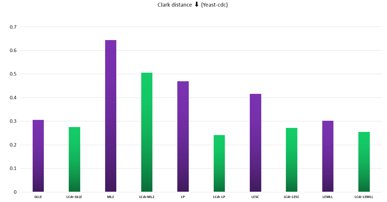
Figure 3: The recovery experiment results visualized measured by Clark$\downarrow$ for each compared algorithm on the controlled Yeast-cdc dataset (with $\alpha$=0.1,$\eta$=10, k=10). For the LE algorithm $\mathcal{F}\in\{$ GLLE,LESC, ML2, LP, LEMLL $\}$, the performance of the $\mathcal{F}$-LCdr is compared against that of $\mathcal{F}.$

4.1.5 LDL Predictive Results

In this section, we verify that the recovered LD can learn a good LDL model. The LDL predictive results were shown in Table 8. Here, IIS-LDL was used as the predictive model to generate the label distributions of testing instances for all the approaches, we chose the same parameter settings as the authors in the paper. From the experimental results, it can be seen that

• The proposed approach ranks 1st in 96.18$\%$ cases, and it achieves superior performance against two algorithms including LESC and LEMLL in all cases.

• The proposed approach achieves superior performance against LP, GLLE, and ML2 in 85.42$\%$ , 93.75$\%$, and 97.92$\%$ cases, respectively.

5 Conclusion

This paper proposed a data augmentation approach to address two problems in LE i.e. $(\mathbf{i})$: logical label do not provide more accurate supervision information and $(\mathbf{ii})$: feature redundancy in LE. To be specific, we used local consistency between instances to generate label-confidence and uses DR techniques to reduce the dimensionality of the feature space to remove redundant information. Combining the above two, we proposed a non-linear LE model. Extensive experimental results demonstrate the effectiveness of the proposed approach consistently outperforms the other five comparing approaches.

References

- Bao et al. [2021] Wei-Xuan Bao, Jun-Yi Hang, and Min-Ling Zhang. Partial label dimensionality reduction via confidence-based dependence maximization. In Proceedings of the 27th ACM SIGKDD Conference on Knowledge Discovery & Data Mining, pages 46–54, 2021.
- Chen et al. [2021] Jingying Chen, Chen Guo, Ruyi Xu, Kun Zhang, Zongkai Yang, and Honghai Liu. Toward children’s empathy ability analysis: Joint facial expression recognition and intensity estimation using label distribution learning. IEEE Transactions on Industrial Informatics, 18:16–25, 2021.
- de Melo et al. [2019] Wheidima Carneiro de Melo, Eric Granger, and Abdenour Hadid. Depression detection based on deep distribution learning. 2019 IEEE International Conference on Image Processing (ICIP), pages 4544–4548, 2019.
- Demsar [2006] Janez Demsar. Statistical comparisons of classifiers over multiple data sets. J. Mach. Learn. Res., 7:1–30, 2006.
- Eisen et al. [1998] Michael B. Eisen, Paul T. Spellman, P O Brown, and David Botstein. Cluster analysis and display of genome-wide expression patterns. Proceedings of the National Academy of Sciences of the United States of America, 95 25:14863–8, 1998.
- Gao et al. [2020] Yongbiao Gao, Yu Zhang, and Xin Geng. Label enhancement for label distribution learning via prior knowledge. In Christian Bessiere, editor, Proceedings of the Twenty-Ninth International Joint Conference on Artificial Intelligence, IJCAI-20, pages 3223–3229. International Joint Conferences on Artificial Intelligence Organization, 7 2020. Main track.
- Geng and Hou [2015] Xin Geng and Peng Hou. Pre-release prediction of crowd opinion on movies by label distribution learning. In International Joint Conference on Artificial Intelligence, 2015.
- Geng and Ling [2017] Xin Geng and Miaogen Ling. Soft video parsing by label distribution learning. Frontiers of Computer Science, 13:302–317, 2017.
- Geng et al. [2020] Xin Geng, Xin Qian, Zeng-Wei Huo, and Yu Zhang. Head pose estimation based on multivariate label distribution. IEEE Transactions on Pattern Analysis and Machine Intelligence, 44:1974–1991, 2020.
- Geng [2016] Xin Geng. Label distribution learning. IEEE Transactions on Knowledge and Data Engineering, 28(7):1734–1748, 2016.
- Gretton et al. [2005] Arthur Gretton, Olivier Bousquet, Alex Smola, and Bernhard Schölkopf. Measuring statistical dependence with hilbert-schmidt norms. In International Conference on Algorithmic Learning Theory, 2005.
- Hou et al. [2016] Peng Hou, Xin Geng, and Min-Ling Zhang. Multi-label manifold learning. In Dale Schuurmans and Michael P. Wellman, editors, Proceedings of the Thirtieth AAAI Conference on Artificial Intelligence, February 12-17, 2016, Phoenix, Arizona, USA, pages 1680–1686. AAAI Press, 2016.
- Ling and Geng [2019] Miaogen Ling and Xin Geng. Indoor crowd counting by mixture of gaussians label distribution learning. IEEE Transactions on Image Processing, 28:5691–5701, 2019.
- Morrison et al. [2018] Shaunna M. Morrison, Feifei Pan, Olivier Charles Gagné, Anirudh Prabhu, Ahmed Eleish, Peter A. Fox, Robert T. Downs, Thomas F. Bristow, Elizabeth B. Rampe, D. F. Blake, David T. Vaniman, Cherie N. Achilles, Doug W. Ming, Albert S. Yen, Allan H. Treiman, Richard V. Morris, Steve J. Chipera, Patricia I. Craig, V. Tu, Nicholas Castle, Philippe C. Sarrazin, D. J. Des Marais, and Robert M. Hazen. Predicting multi-component mineral compositions in gale crater, mars with label distribution learning. 2018.
- Shao et al. [2018] Ruifeng Shao, Ning Xu, and Xin Geng. Multi-label learning with label enhancement. In IEEE International Conference on Data Mining, ICDM 2018, Singapore, November 17-20, 2018, pages 437–446. IEEE Computer Society, 2018.
- Si et al. [2022] Shijing Si, Jianzong Wang, Junqing Peng, and Jing Xiao. Towards speaker age estimation with label distribution learning. ICASSP 2022 - 2022 IEEE International Conference on Acoustics, Speech and Signal Processing (ICASSP), pages 4618–4622, 2022.
- Tang et al. [2020] Haoyu Tang, Jihua Zhu, Qinghai Zheng, Jun Wang, Shanmin Pang, and Zhongyu Li. Label enhancement with sample correlations via low-rank representation. In AAAI Conference on Artificial Intelligence, 2020.
- Wu et al. [2019] Xiaoping Wu, Ni Wen, Jie Liang, Yu-Kun Lai, Dongyu She, Ming-Ming Cheng, and Jufeng Yang. Joint acne image grading and counting via label distribution learning. 2019 IEEE/CVF International Conference on Computer Vision (ICCV), pages 10641–10650, 2019.
- Xu et al. [2018] N. Xu, An Tao, and Xin Geng. Label enhancement for label distribution learning. IEEE Transactions on Knowledge and Data Engineering, 33:1632–1643, 2018.
- Xu et al. [2019a] Ning Xu, Yun-Peng Liu, and Xin Geng. Label enhancement for label distribution learning. IEEE Transactions on Knowledge and Data Engineering, 33(4):1632–1643, 2019.
- Xu et al. [2019b] Ning Xu, Jiaqi Lv, and Xin Geng. Partial label learning via label enhancement. In The Thirty-Third AAAI Conference on Artificial Intelligence, AAAI 2019, The Thirty-First Innovative Applications of Artificial Intelligence Conference, IAAI 2019, The Ninth AAAI Symposium on Educational Advances in Artificial Intelligence, EAAI 2019, Honolulu, Hawaii, USA, January 27 - February 1, 2019, pages 5557–5564. AAAI Press, 2019.
- Xu et al. [2020] Ning Xu, Jun Shu, Yun-Peng Liu, and Xin Geng. Variational label enhancement. 119:10597–10606, 2020.
- Xu et al. [2021] Ning Xu, Yun-Peng Liu, and Xin Geng. Label enhancement for label distribution learning. IEEE Trans. Knowl. Data Eng., 33(4):1632–1643, 2021.
- Xu et al. [2022] Ning Xu, Jun Shu, Renyi Zheng, Xin Geng, Deyu Meng, and Min-Ling Zhang. Variational label enhancement. IEEE Transactions on Pattern Analysis and Machine Intelligence, pages 1–15, 2022.
- Yang et al. [2017] Jufeng Yang, Ming Sun, and Xiaoxiao Sun. Learning visual sentiment distributions via augmented conditional probability neural network. In Satinder Singh and Shaul Markovitch, editors, Proceedings of the Thirty-First AAAI Conference on Artificial Intelligence, February 4-9, 2017, San Francisco, California, USA, pages 224–230. AAAI Press, 2017.
- Yang et al. [2018] Jufeng Yang, Liyi Chen, Le Zhang, Xiaoxiao Sun, Dongyu She, Shao-Ping Lu, and Ming-Ming Cheng. Historical context-based style classification of painting images via label distribution learning. Proceedings of the 26th ACM international conference on Multimedia, 2018.
- Zhang and Zhou [2010] Yin Zhang and Zhi-Hua Zhou. Multilabel dimensionality reduction via dependence maximization. ACM Transactions on Knowledge Discovery from Data (TKDD), 4(3):1–21, 2010.
- Zhang et al. [2021] Min-Ling Zhang, Qian-Wen Zhang, Jun-Peng Fang, Yu-Kun Li, and Xin Geng. Leveraging implicit relative labeling-importance information for effective multi-label learning. IEEE Trans. Knowl. Data Eng., 33(5):2057–2070, 2021.
- Zhao et al. [2022] Xingyu Zhao, Yuexuan An, Ning Xu, and Xin Geng. Fusion label enhancement for multi-label learning. In Lud De Raedt, editor, Proceedings of the Thirty-First International Joint Conference on Artificial Intelligence, IJCAI-22, pages 3773–3779. International Joint Conferences on Artificial Intelligence Organization, 7 2022. Main Track.
- Zheng et al. [2020] Qinghai Zheng, Jihua Zhu, Haoyu Tang, Xinyuan Liu, Zhongyu Li, and Huimin Lu. Generalized label enhancement with sample correlations. IEEE Transactions on Knowledge and Data Engineering, 35:482–495, 2020.
- Zhou et al. [2022] Xiuzhuang Zhou, Zeqiang Wei, Min Xu, Shanhu Qu, and Guodong Guo. Facial depression recognition by deep joint label distribution and metric learning. IEEE Transactions on Affective Computing, 13:1605–1618, 2022.