Transfer-Learned Potential Energy Surfaces: Towards Microsecond-Scale Molecular Dynamics Simulations in the Gas Phase at CCSD(T) Quality
Abstract
The rise of machine learning has greatly influenced the field of computational chemistry, and that of atomistic molecular dynamics simulations in particular. One of its most exciting prospects is the development of accurate, full-dimensional potential energy surfaces (PESs) for molecules and clusters, which, however, often require thousands to tens of thousands of ab initio data points restricting the community to medium sized molecules and/or lower levels of theory (e.g. DFT). Transfer learning, which improves a global PES from a lower to a higher level of theory, offers a data efficient alternative requiring only a fraction of the high level data (on the order of 100 are found to be sufficient for malonaldehyde). The present work demonstrates that even with Hartree-Fock theory and a double-zeta basis set as the lower level model, transfer learning yields CCSD(T)-level quality for H-transfer barrier energies, harmonic frequencies and H-transfer tunneling splittings. Most importantly, finite-temperature molecular dynamics simulations on the sub-s time scale in the gas phase are possible and the infrared spectra determined from the transfer learned PESs are in good agreement with experiment. It is concluded that routine, long-time atomistic simulations on PESs fulfilling CCSD(T)-standards become possible.
University of Basel]Department of Chemistry, University of Basel, Klingelbergstrasse 80 , CH-4056 Basel, Switzerland. University of Basel]Department of Chemistry, University of Basel, Klingelbergstrasse 80 , CH-4056 Basel, Switzerland.
1 Introduction
Over the past decade, machine learning-based approaches have
persistently influenced the field of computational chemistry as a
whole and that of atomistic molecular dynamics (MD) simulations in
particular.1, 2, 3
Machine learning (ML) approaches begin to be routinely used in areas
ranging from reaction planning4, 5,
to drug design6, 7 and to the
construction and use of accurate local and global potential energy
surfaces
(PESs).8, 9, 3, 10
Common to all these applications is that they are data-driven,
i.e. they depend on the amount but also on the quality of the
available data on which the statistical models are trained. With
respect to the underlying models themselves, much flexibility exists,
encompassing kernel- or neural network-based approaches with a wide
range of architectures and specific design
choices.11, 8, 9, 2, 3
The construction of a multidimensional PES suitable for
routine and robust MD simulations remains a challenging
task.12 An established approach consists of
precomputing reference energies and forces from electronic structure
methods at suitable and affordable levels of theory for a given
molecule or system, also often with particular applications such as
various spectroscopies or reaction dynamics in mind. Traditionally,
these energies were used to fit predetermined parametrized forms which
in turn not only provide the total energy of the system but also
analytical derivatives for forces required in MD simulations. The
difficulty in such approaches consists in “guessing” sufficiently
flexible forms of the parametrization to capture local and global
features of the PES alike. Also, such parametrized fits are often
highly nonlinear which is another challenge, in particular for
high-dimensional PESs.
ML methods, including (reproducing)
kernel13, 14 or neural network (NN)
approaches15, 16, have been long
known to be flexible function
approximators17. It is precisely this
flexibility that is also beneficial for the representation of molecular
PESs which can have a wide range of topographies and designing
parametrizations suitable for capturing all relevant features becomes
increasingly difficult.
Here, the construction, improvement and use of reactive PESs in
ring-polymer instanton (RPI) calculations and MD simulations is
discussed with the purpose of illustrating practical aspects and
probing the quality of the resulting surfaces. The method employed to
improve PESs from a lower level (LL) to a higher level (HL) of theory
is transfer learning
(TL)18, 19, 20 which
is rooted in the notion that the overall topographies of molecular
PESs at different levels of theory are often similar. As an example,
it is often found that the number of local minima is comparable or
even identical if quantum chemical methods at different levels of
theory are employed, whereas the geometrical structures of course
differ. This topographical similarity can be exploited in TL
approaches in that measured amounts of HL information are used to
locally distort the model based on LL data. One particular focus in
the present work is on studying the influence of the level of
electronic structure theory used to construct the surrogate LL model
on the quality of the HL PES and making best use of the data
generated. To the best of our knowledge this contribution presents the
first systematic analysis of the influence of the LL PES in TL of
global reactive molecular potential energy surfaces.
Malonaldehyde (MA) is a well-studied molecule
experimentally
21, 22, 23, 24, 25, 26, 27, 28
and from
computations29, 30, 31, 32, 33 and provides a
suitable benchmark system for the present work and recent
results34 serve as a reference. The
properties used for
evaluating the quality of the final PESs include energies
(e.g. RMSE() from comparison to ab initio reference),
barrier heights for hydrogen transfer (H-transfer), harmonic frequencies
(allowing comparison with
experiments25, 35 and
ab initio results34), and
tunneling splittings (allowing comparison to
experiment21, 22, 23
and
literature34). Alternative/additional
observables include H-transfer rates and infrared spectra inferred
from MD simulations which can also be compared with experiment.
The present work is structured as follows. First, the methods
including the NN-based representation of the PESs and TL are
discussed. Then, the results comprising out of sample errors, energy
barriers, harmonic frequencies and tunneling splittings as well as the
results from an aggregate of 1.5 s of MD simulations are
presented. Finally, the results are discussed in a broader context and
compared to previous experiments and computational work.
2 Methods
This section introduces the employed ML approaches, the data generation procedure, RPI theory, the MD simulation protocol, analysis and computation of the observables.
2.1 Machine Learning
All full-dimensional, reactive PESs used in this work are represented by a high dimensional, message-passing36 NN of the PhysNet type15. PhysNet predicts energies, forces and dipole moments for arbitrary molecular configurations from a feature vector that is learned to describe the local chemical environment (here, up to a cutoff radius Å) of each atom . The total potential energy of a molecule with atoms for a given geometry is given by
| (1) |
where are the atomic contributions to the total energy of the molecule, is Coulomb’s constant and the second term describes pairwise electrostatic contributions. Note that the partial charges are corrected for charge conservation and that the electrostatic contribution is damped at small inter-atomic distances due to the singularity (for details see Reference15). The forces and Hessians are obtained analytically from reverse mode automatic differentiation37 as implemented in Tensorflow38 and the dipole moment is calculated as
| (2) |
The learnable parameters in PhysNet were fit to reference ab
initio energies, forces and dipole moments following the procedure
described in Reference 15. Note that the
partial charges were adapted to best reproduce the dipole moment
from the ab initio calculations.
Recently, TL20, 39 and related approaches including -ML40, 41, 42 have become very popular and successful in improving a given LL PES to a HL of theory. At its core, TL builds on the knowledge acquired by solving one task (representing the LL PES) to solve a new, related task (representing the HL PES).20 In practice, the parameters of the LL PES are used as a good initial guess and are fine-tuned with little, though judiciously, chosen HL information. In this work, all parameters of PhysNet were allowed to change in the TL step.
2.2 Ab Initio Data
All molecular structures that were used to in the fitting procedure of PhysNet
were available from earlier work33 and their sampling
process is described in detail in Reference 33. The
data set contains structures for MA, acetoacetaldehyde (3-oxobutanal),
acetylacetone (pentan-2, 4-dion) as well as a total of 49
substructures as motivated by the ”amon”
approach.43 An initial set of structures was
generated by running Langevin dynamics at 1000 K using the
semi-empirical PM7 method44 as implemented
in MOPAC45. Next, ab initio energies,
forces and dipole moments were determined at the MP2/aug-cc-pVTZ
(aVTZ) level of theory using MOLPRO46 and were used to
train two preliminary PhysNet models. The preliminary models were
then used to suitably augment the data set using adaptive
sampling47. The final data set contained MP2/aVTZ
level energies, forces and molecular dipole moments for a total of
71 208 structures including all three molecules and their amons. This
PES is referred to as PhysNetMP2.
To be able to study the influence of the LL on the quality of the HL,
the data set containing 71 208 structures from earlier
work33 was recalculated at two additional ”low” levels
of theory, namely HF/cc-pVDZ (VDZ) and B3LYP/aVTZ using
MOLPRO46. The two new data sets are used to learn
representations of the PES using PhysNet and are termed PhysNetHF and PhysNetB3LYP, respectively. The relative CPU times
for the ab initio calculations (that include energies, forces
and dipole moments) are roughly 1:10:170:4000 for the HF/VDZ,
B3LYP/aVTZ, MP2/aVTZ and CCSD(T)/aVTZ levels of theory,
respectively.
The CCSD(T)/aVTZ level of theory was chosen as higher level of theory,
which is computationally much more demanding, and will serve as target
in the TL step.34 Although the
determination of forces and dipole moments is roughly an order of
magnitude more expensive than an energy-only calculation, the
information gained from including gradients (27 components for
malonaldehyde) and dipole moments is considerable. The data set sizes
employed in the TL step of the present work include (corresponding to TL0, TL1, TL2 and TLext)
MA structures. Except for (which corresponds to an extended
data set that contains all HL
information.34) the MA structures were
augmented iteratively and are specifically chosen to ideally
cover all relevant spatial
regions (i.e. structures on and around the minimum energy path, instanton
path, global minimum and transition state)
of the PESs that were found to be important for the
determination of the tunneling
splitting34. The resulting TL PESs
corresponding to the LL models (PhysNetHF, PhysNetB3LYP or PhysNetMP2) are termed TL with
x[HF, B3LYP, MP2] and y[0, 1, 2, ext].
2.3 Ring-Polymer Instanton Theory
The ring polymer instanton (RPI) method offers a semiclassical approximation for computing tunneling splittings in molecular systems.48, 49, 50, 51 Instanton theory, which is closely related to the WKB approximation52 in a one-dimensional model can be applied to multidimensional systems as well. It identifies the optimal tunneling pathway, called the instanton, by locating the imaginary-time path connecting two degenerate wells that minimizes the action, . To determine the instanton, a ring-polymer optimization technique is used to discretize the path into beads and take the limit as . is then determined using information from the potential energy of and distances between neighboring beads along the instanton path (IP). Usually, the instanton path does not pass through the saddle point of the reaction and is different from the minimum energy path. In addition to the IP, a contribution characterizing the fluctuations around the path needs to be computed to second order which necessitates the availability of Hessians at each bead. The tunneling splitting is then given by
| (3) |
Full technical details regarding the RPI approach are given, e.g., in
References53 and
54.
2.4 Molecular Dynamics Simulations
The MD simulations evaluated in this work were all performed using
PhysNet PESs and using the atomic simulation environment
(ASE55) in Python. Starting from a given PES, the
structure of MA was first optimized to its minimum energy structure
before random momenta were drawn from a Maxwell-Boltzmann distribution
corresponding to K and assigned to the atoms. The MD
simulations were carried out in the NVE ensemble using the
Velocity Verlet algorithm and a time step of fs to
conserve energy as bonds involving hydrogen were flexible. The system
was first allowed to equilibrate for 2.5 ps and was followed by a
production simulation of 250 ps each. At each temperature and using a
representative HL PES for each class of TL PESs, 1000 independent
trajectories were run using different initial momenta. This
accumulated to a total of 750 ns simulation time per temperature
.
The MD simulations were used to estimate H-transfer rates, which were calculated as the accumulated number of H-transfers divided by the accumulated total simulation time, . A H-transfer was considered complete whenever the H-atom transfers from being closer to one O-Atom to the other (e.g. when changes to ), although other criteria exist and have been used.56 For the present work the details of the criterion are of less interest because only the relative rates from simulation based on the different PESs is analyzed. The same trajectories were also used to compute infrared (IR) spectra from the Fourier transform of the dipole-dipole auto-correlation function,57 according to
| (4) |
Here, the Fourier transform was further corrected by a quantum
correction factor58 .
3 Results
The following section presents first the results derived from the LL PESs for MA. This includes out of sample errors, energy barriers and harmonic frequencies as determined from the LL PESs including the comparison to their ab initio references, and tunneling splittings. This is followed by the results for the HL PESs.
3.1 Quality of LL PESs
The LL PESs generated at three different levels of theory including
HF, B3LYP and MP2 (PhysNetHF, PhysNetB3LYP and
PhysNetMP2) are evaluated on a test set containing 9208
structures. The mean absolute (MAE) and root mean squared (RMSE)
errors on energies and forces are summarized in
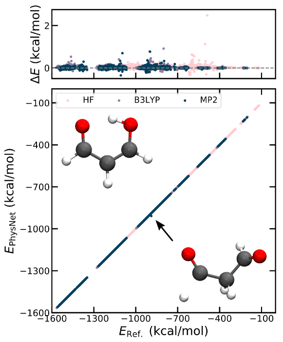
Table 1. MAE() for all models are below
0.05 kcal/mol and are lowest for PhysNetMP2 (0.02 kcal/mol).
Conversely, the RMSE() for PhysNetMP2 is highest (a factor
of larger than for PhysNetHF and PhysNetB3LYP). The MAE() are within kcal/mol/Å for all
three LL PESs while the RMSE() differ by kcal/mol/Å
at most. The correlation and the errors of the PhysNet energies with
respect to the respective reference ab initio values are
shown in Figure 1 for the test set.
The barrier for H-transfer from the ab initio calculations varied
between 9.96, to 2.98 and 2.74 kcal/mol for the HF, B3LYP and MP2
level of theory, respectively. Excellent fitting accuracy with respect
to ab initio reference is found for all LL PESs with the
largest absolute deviation of kcal/mol for PhysNetMP2. These barrier heights compare with 4.03 kcal/mol and 4.09
kcal/mol from high-level CCSD(T) calculations of different
flavours.8, 31
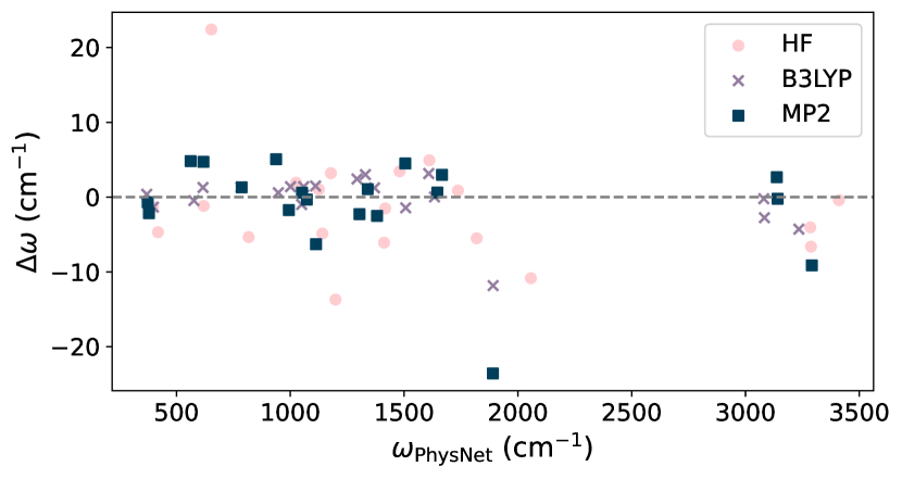
Harmonic frequencies constitute an additional measure for the accuracy
of a PES around a stationary point. The MAEs and the RMSEs for the
harmonic frequencies of the global minimum of MA for all LL PESs are
reported in Table 1. While the MAEs (RMSEs)
for all LL PESs are below 5 (7) cm-1, the errors for
PhysNetHF are slightly larger by approximately a factor of 2
compared to PhysNetB3LYP and PhysNetMP2, which are
within 0.1 cm-1 of one another. The actual deviation of the
PhysNet harmonic frequencies with respect to their reference is shown
in Figure 2 for the global
minimum of MA. The largest difference is found for PhysNetHF
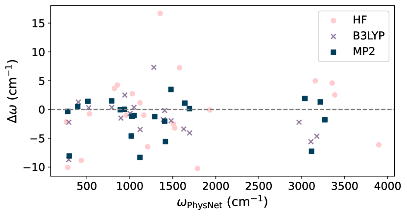
with a deviation of cm-1. For the H-transfer transition state,
the MAEs (RMSEs) are all below 6 (9) cm-1 (see
Table S2). Here, PhysNetB3LYP yields the most accurate frequencies with a MAE and RMSE of
2.3 and 3.6 cm-1, respectively. A comprehensive list of the
harmonic frequencies for the minimum and H-transfer transition state as
calculated on the LL PhysNet PESs and their ab initio
reference are given in Tables S1 and
S2, respectively.
As one of the target observables, that allows a comparison to
experiment21, 22, 23,
the tunneling splittings for H-transfer and deuterium transfer (D-transfer)
are calculated for all LL PESs. The tunneling
splitting is exquisitely sensitive to the quality and accuracy of the
PES along and around the instanton path comprising the minimum energy
structure and the region near the transition state. The
tunneling splitting for H-transfer, , ranges from , to
71.1 and to 96.3 cm-1 for PhysNetHF, PhysNetB3LYP and PhysNetMP2. Similarly, the tunneling splittings
for D-transfer, , are 9.9 , 12.8 and
18.8 cm-1. This compares with
experimentally21, 22 determined
tunneling splittings of 21.583 and 2.915 cm-1 for H-transfer and D-transfer,
respectively, and RPI calculations at CCSD(T) quality (TL +
RPI)34 of 25.3/3.7 cm-1. The
hydrogen tunneling splitting spans more than three
orders of magnitude and impressively illustrates its exquisite
sensitivity to the shape and accuracy of the PES.
| HF | B3LYP | MP2 | |
| MAE()/(kcal/mol) | 0.046 | 0.028 | 0.020 |
| RMSE()/(kcal/mol) | 0.063 | 0.040 | 0.210 |
| MAE()/(kcal/mol/Å) | 0.067 | 0.059 | 0.062 |
| RMSE()/(kcal/mol/Å) | 0.177 | 0.141 | 0.242 |
| /(kcal/mol) | 10.00 | 3.02 | 2.79 |
| /(kcal/mol) | 9.96 | 2.98 | 2.74 |
| MAE()/(cm-1) | 4.8 | 2.6 | 2.5 |
| RMSE()/(cm-1) | 6.2 | 3.5 | 3.6 |
| /(cm-1) | 0.0358 | 71.1 | 96.3 |
| /(cm-1) | 0.000991 | 12.8 | 18.8 |
3.2 Performance of the TL PESs
The quality of the HL, transfer-learned PESs TL with
x[HF, B3LYP, MP2] and y[0, 1, 2, ext] starting form three
different LL PESs is broadly evaluated next. On account of the small
HL data set sizes (including for TL0,
TL1, TL2 and TLext), each TL is repeated 10 times on
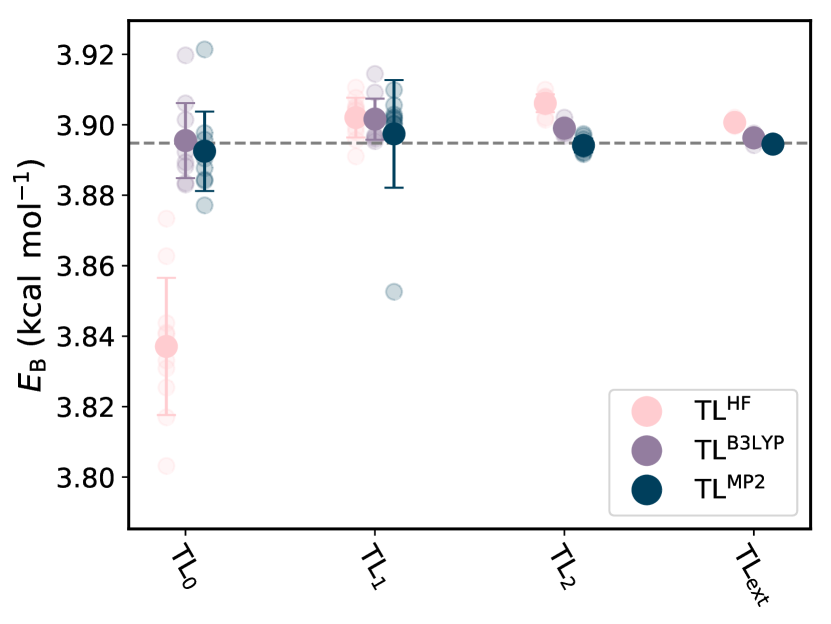
different splits of the data. The energy barriers for the
different HL PESs together with their variation are shown in
Figure 3 for all TLs (transparent
circles). Their averages and standard deviations are indicated as
opaque circles and error bars, respectively. The gray dashed line
corresponds to the ab initio CCSD(T)/aVTZ energy barrier
determined in previous work34. While
TL and TL (i.e. requiring only 25 data
points) already yield within 0.003 kcal/mol of the ab
initio CCSD(T)/aVTZ barrier, the deviation of kcal/mol
for TL is slightly larger. For all larger data set sizes,
the energy barrier for H-transfer of the HL PESs are accurate and equal among
themselves to within kcal/mol. Overall, TL from all LL
models yields HL models with for H-transfer to within
kcal/mol of the reference value from ab initio
CCSD(T)/aVTZ calculations determined in previous
work34. This ab initio
CCSD(T)/aVTZ barrier of 3.895 kcal/mol compares to values of 4.09 and
4.03 kcal/mol as obtained at the CCSD(T)/aug-cc-pV5Z (optimization
carried out at CCSD(T)/aVTZ level) and fc-CCSD(T) (F12*)/def2-TZVPP
level of theory,
respectively.8, 31
The energy barrier for H-transfer is a local, rather low
dimensional property of a PES. Conversely, harmonic frequencies for
stationary points probe the curvature of the PES in all
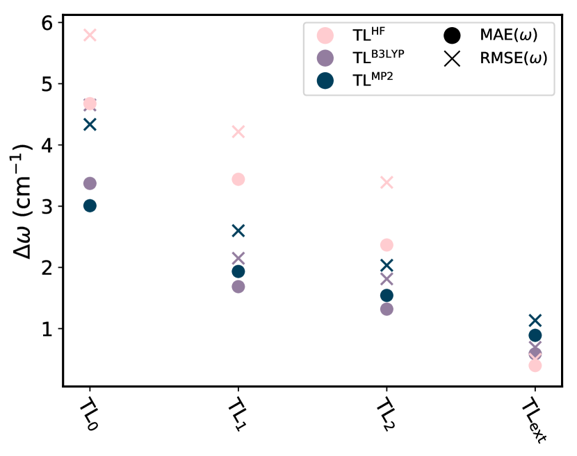
directions. Figure 4 shows the MAE and
RMSEs of ensemble predictions (i.e. an average over 10 TLs) for the
global minimum of MA of TLHF, TLB3LYP and TLMP2 for the different TL data set sizes (i.e. 25, 50, 100, 862).
Averaged errors below 6 cm-1 are achieved for all HL PESs with as
little as 25 data points. TL with 100 CCSD(T)/aVTZ data
points the MAEs (RMSEs) are further reduced to 2.4, 1.3 and 1.5 (3.4,
1.8 and 2.0) cm-1 for TL, TL and
TL, respectively. The RMSEs between the ab
initio HF/B3LYP/MP2 harmonic frequencies and the high-level CCSD(T)
frequencies are 177, 28 and 21 cm-1 for HF, B3LYP and MP2,
respectively, and provides an impression by how much the shape of the
LL PESs need to adjust around the minimum at the TL
step.
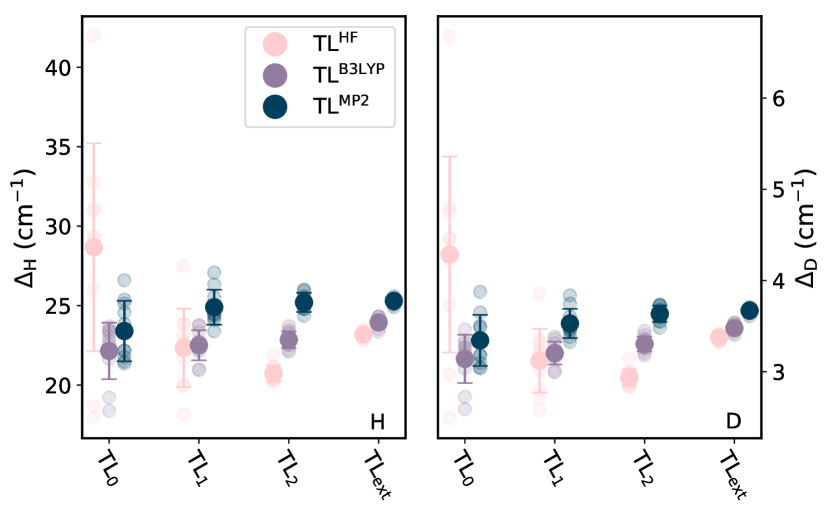
The tunneling splitting is sensitive to the local dynamics and the
PES’s topology around the H-transfer instanton path. Hydrogen and deuterium
tunneling splittings were used as target observables in recent work
for the iterative and systematic construction of different data sets
based on PhysNetMP2. 34
Figure 5 presents the tunneling splittings for
H-transfer and D-transfer as calculated from all different HL PESs (TL to
TL). Again, their averages and standard
deviations are shown as opaque circles and error bars,
respectively. As had been found for , the fluctuation is
largest for TL with tunneling splittings ranging from
to 42 cm-1. This fluctuation is smaller by a factor of
for both TL and TL. For TL2
the fluctuation among the three classes of HL PES become
comparable. Average of 20.7, 22.9 and 25.2 cm-1
are found for TL, TL and TL. Increasing the data set size to 862 (TLext)
further reduces both the differences within the classes and the
standard deviation of the ensemble predictions. Here, average
of 23.2, 23.9 and 25.3 cm-1 are found for
TL, TL and TL, respectively. It is noted, that
from TLMP2 only marginally changed upon increasing the TL
data set size from 100 to 862 (TL2 to TLext). Similar
observations hold for D-transfer, which indicates that TL is
basically converged with MP2 as the LL model.
3.3 Molecular Dynamics on the HL PESs
Further evaluations focus on dynamical properties derived from MD
simulations carried out on the HL PESs. As a TL data set size of 100
CCSD(T) data points (TL2) is a very realistic scenario for final
predictions (i.e. allows to check for convergence of the results and a
small enough data set size to be amenable also for larger systems), a
representative PES (from the 10 independent TL executions) was chosen
for each of the three TL classes (i.e. TL, TL and TL).
H-transfer rates obtained from counting H-transfers and dividing by total
simulation time from the MD simulations at 300 and 500 K are reported
in Table 2. The rates at both temperatures
agree to approximately 30 % and correspond to (34) transfers
per ns at 300 (500) K. It is interesting to note that the trend at
300 K (i.e. lowest rate for TLHF followed by LB3LYP
and TLMP2) reverses at 500 K. Overall, the rates for TLB3LYP and TLMP2 are more similar to one another.
| (1/ns) | 300 K | 500 K |
|---|---|---|
| TLHF | 0.9 | 41.0 |
| TLB3LYP | 1.1 | 32.1 |
| TLMP2 | 1.4 | 33.9 |
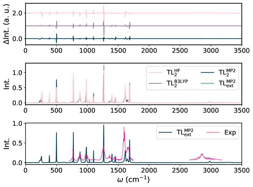
The simulation run at 300 K were further used to compute IR spectra as calculated from the dipole-dipole autocorrelation function, see Figure 6 (middle panel) for TL, TL and TL. As additional reference, an IR spectrum was also calculated on TL which, starting from the MP2 LL PES, has been trained on an extended TL data set containing 862 CCSD(T) data points and is thus expected to yield results closest to simulations on a -hypothetical - PhysNet PES trained on CCSD(T)/aVTZ reference data. The spectra derived from the dynamics on the HL PESs are very similar with one another. Single deviations can, e.g. be found at cm-1 or at cm-1, where TL has no or only a small fraction of the intensity in comparison to the other spectra, respectively. The difference spectra (for = {HF, B3LYP, MP2}) shown in the top panel of Figure 6 illustrate differences between TL, TL and TL on the one hand and TL as the reference. The smallest deviations are found for TL, as expected, while larger differences are found for TLHF and TLB3LYP. For example, the intensity of the peak at cm-1 is twice as large for TL and the line positions of TL and TL at cm-1 are shifted to the blue by cm-1 compared to TL and TL, respectively. The bottom panel shows the direct comparison of TLMP2 with the experimental spectrum determined in Reference 35 and illustrates the excellent agreement for frequencies between 500 and 1500 cm-1. Somewhat larger deviations are found for peaks at and 2900 cm-1. Aside from obtaining correct peak positions from the calculated IR spectra, the infrared intensities are also found to remarkably well capture the trend visible in the experiment.
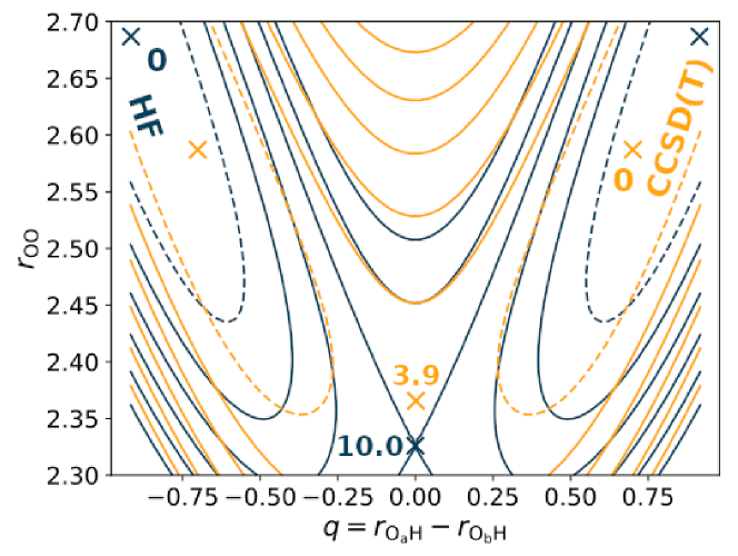
4 Discussion
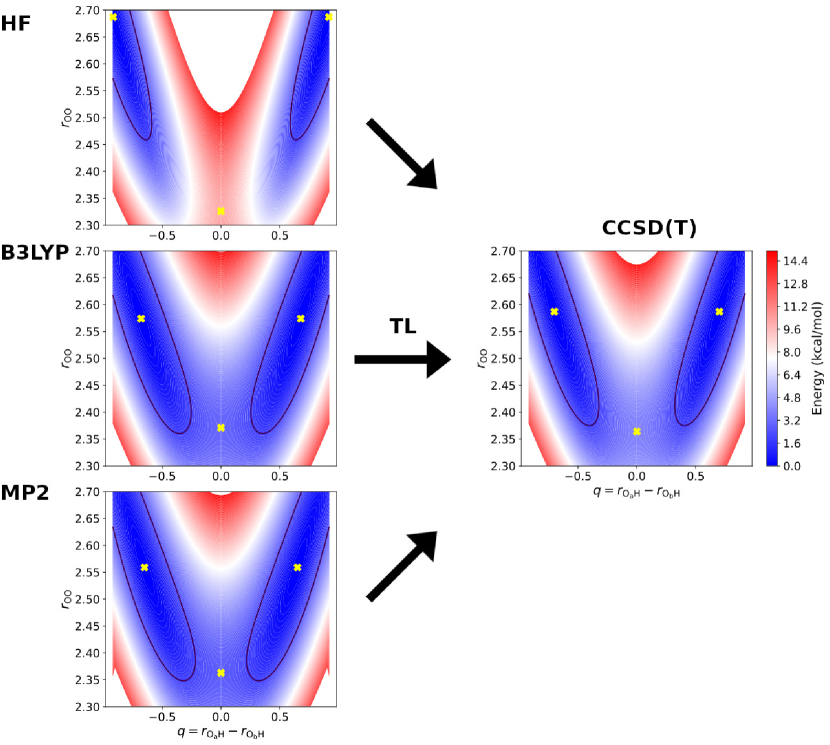
The present study considered TL from a range of LL methods to CCSD(T)
using variable amounts of HL information. For the molecule considered
here - malonaldehyde - the relative computational cost of the LL
methods ranged from 1 to but the qualities of the
transfer-learned HL PESs - as inferred from the observables considered
- were almost identical if 50 to 100 HL data points were used in the
TL step. Two-dimensional projections of the LL PESs compared with the
best HL target PES are reported in Figure
7. This provides a low-dimensional
impression of the amount of reshaping that is conveyed by the TL
step because all TL-PESs from the three LL reference
calculations yield comparable final PESs.
Properties for which the performance of the transfer learned PESs were
evaluated and compared included the barrier for H-transfer, the
tunneling splittings, harmonic frequencies and IR spectra from
finite-temperature MD simulations in the gas phase. All results
suggest that the level of theory of the LL PES has only a minor
influence on the quality of the resulting HL PES, although starting
from a ”better LL PES” (e.g. B3LYP/aVTZ) might have slight advantages
such as a shorter training time for TL. As an example, TL from
PhysNetHF to CCSD(T)/aVTZ based on 100 points required
one order of magnitude more epochs than PhysNetB3LYP or
PhysNetMP2. Thus, although transfer learning a surrogate model at the HF/aVDZ
level yields a HL model of almost identical quality compared to
TL and TL, the B3LYP/aVTZ
level of theory may offer the best cost/accuracy ratio.
Starting from ”equivalent” LL PESs in terms of representation error, a
HL PESs of gold standard CCSD(T) quality was sought after and
generated using TL. As an example for the performance of the TL
step, normal mode frequencies are considered. The three LL
PES achieve outstanding accuracy with respect to the frequencies from
ab initio normal mode calculations at the respective levels
of theory for both, the minimum energy structure and for the
H-transfer transition state. PhysNetB3LYP is most accurate
with MAE() = 2.6, RMSE cm-1 and a maximum
absolute error of cm-1 for the global minimum of
MA. This compares favourably with state of the art art PESs for
molecules of similar sizes. A recent permutationally invariant
polynomial (PIP) PES for tropolone yields MAE()min
between 1.7 and 12.7 cm-1 the reported MAE()TS
ranges from 8.4 cm-1 to 18.6 cm-1, depending on chosen PIP
basis and other method-specific
parameters.59. PIP- and PhysNet-based
PESs for the formic acid dimer find MAE()min of 14.9
and 6.4 cm-1,
respectively.60, 61, 62 Comparing
the harmonic frequencies from the LL PESs (HF, B3LYP and MP2) with the
target level of theory, CCSD(T), reflects the amount of reshaping of
the PES that is required in the TL step to reach the reported
performance. This needs to be compared with differences in the
harmonic frequencies at the ab initio HF/B3LYP/MP2 levels
compared with the CCSD(T) frequencies34
with an RMSE of 177, 28 and 21 cm-1 for HF, B3LYP and MP2,
respectively. TL with only 100 HL data points correctly reshaped the
LL PESs with a MAE and RMSE cm-1
(i.e. the same accuracy as for the most accurate LL PES, PhysNetB3LYP, trained on several ten thousand structures), respectively,
and impressively illustrates the data efficiency of TL. This translates
into improvements of 1 to 2 orders of magnitude in accuracy for normal
mode frequencies between reference and transfer-learned models
It is also valuable to consider the accuracy of the computed harmonic
frequencies in light of the computational effort to obtain such
frequencies (especially at the CCSD(T) level of theory) based on
standard ab initio techniques. As is well established in the
community, optimizations and frequency calculations at the CCSD(T)
level of theory are tremendously time and resource intensive,
especially for larger and complex systems.
Starting from, e.g. PhysNetB3LYP, required only 100 HL
CCSD(T) data points (that include energies, forces and dipole moments)
to achieve close to spectroscopic accuracy (i.e. more than 60 % of
the frequencies with sub-1 cm-1 accuracy and a maximum deviation
of cm-1 with respect to ab initio CCSD(T)
reference). ML methods, especially in combination with data-efficient
TL or related -ML approaches, therefore offer an attractive
time-saving alternative as has been demonstrated here. This is
highlighted by recent ab initio LCCSD(T)-F12/cc-pVTZ-F12
calculations for 15-atom tropolone, for which the optimization and
frequency calculation took 73 days on 12
cores.63
The present findings underscore the importance for a sufficiently
detailed LL model when aiming to construct a high-quality, versatile
PES based on as little HL data as possible. This is shown by
comparing to a model trained on the TL2 (100 CCSD(T) data points)
data set from scratch, i.e. without pre-training. The resulting model is
predicts the energy barrier moderately well (a deviation of
kcal/mol with respect to reference), but has significantly
larger errors for harmonic frequencies (i.e. MAE() cm-1) than all TL models. In addition, starting
MA structure optimization close to the stationary point is
necessary for meaningful results. As anticipated, the attempt to run a MD
simulation on such a PES fails entirely after a few time steps even at
a rather low temperature of 300 K, which renders the PES unsuitable
for dynamics studies.
Contrary to the model trained from scratch, TL enables to obtain a
very HL representation of a global PES with very limited HL data
points and, thus, allows to carry out dynamical assessments of a
system. In this contribution this has been illustrated for the IR
spectrum of MA and compared to experiment, for which good agreement is
found. Since the TL data set contains only few structures which are
chosen rather close to the global minimum and H-transfer transition state, it
is conceivable that elevated temperatures lead to sampling structures
with stronger distortions which are not fully covered by the TL data
set. To the best of our knowledge, it is yet to be examined how a LL
PES is transformed in regions where no TL data is supplied and
presents a promising avenue for further investigation. Nevertheless,
this very attractive route employing TL to obtain HL PESs allows
CCSD(T)-quality MD simulations on the microsecond time scale for
medium sized molecules. As an indication for the reduction in
computing time achieved for MA it is noted that 1 ns of ML/MD
simulation takes 12 CPU hours whereas the same simulation with ab initio MD simulations at the CCSD(T)/aVTZ level would take
hours, i.e. longer, i.e. they are unfeasible. Of course such comparisons depend
somewhat on the computer architecture and implementation used, but
serve as an illustration that approaches as those discussed in the
present work open possibilities to combine accuracy, system size and
simulation lengths to approache CCSD(T)-level quality in subs simulations that were unachievable with more established
methods. With regards to PES generation, TL
alleviates the problem of requiring thousands to tens of thousands of
HL ab initio data points. This is a major step forward making
highest levels of theory accessible. The adaptation of this approach
to ML/MM simulations is a promising avenue towards stable, energy
conserving, long-time quantitative condensed phase simulations.
5 Conclusion
The present work demonstrated that even with HF/aVDZ as the LL model
high-quality full dimensional reactive PESs at the CCSD(T)/aVTZ level
can be obtained through TL. Given a shape of the PES
from a very economical level of theory, TL reshapes the
LL PES to a HL PES from which observables agree favourable with both,
experiments and models directly trained at the HL. Because the
computational effort to evaluate energies and forces of a PES based on
a NN does not depend on the level of ab initio theory used to
conceive the representation, extensive and routine sub-s gas-phase
ML//MD and condensed-phase ML/MM//MD simulations with the solvent
treated with molecular mechanics become possible and are in reach.
Data Availability Statement
The MP2/aVTZ data set taken from previous work33 is available on zenodo (\urlhttps://zenodo.org/record/3629239#.ZBhlJ47MJH4) and the PhysNet codes are available at \urlhttps://github.com/MMunibas/PhysNet. Additional data sets generated during and/or analysed during the current study are available from the authors upon reasonable request.
Acknowledgments
The authors gratefully acknowledge partial financial support from the
Swiss National Science Foundation through grant , the
NCCR-MUST, and from the University of Basel.
References
- Keith et al. 2021 Keith, J. A.; Vassilev-Galindo, V.; Cheng, B.; Chmiela, S.; Gastegger, M.; Müller, K.-R.; Tkatchenko, A. Combining machine learning and computational chemistry for predictive insights into chemical systems. Chem. Rev. 2021, 121, 9816–9872
- Meuwly 2021 Meuwly, M. Machine learning for chemical reactions. Chem. Rev. 2021, 121, 10218–10239
- Unke et al. 2021 Unke, O. T.; Chmiela, S.; Sauceda, H. E.; Gastegger, M.; Poltavsky, I.; Schütt, K. T.; Tkatchenko, A.; Müller, K.-R. Machine learning force fields. Chem. Rev. 2021, 121, 10142–10186
- Coley et al. 2018 Coley, C. W.; Green, W. H.; Jensen, K. F. Machine learning in computer-aided synthesis planning. Acc. Chem. Res. 2018, 51, 1281–1289
- Chen et al. 2020 Chen, B.; Li, C.; Dai, H.; Song, L. Retro*: Learning Retrosynthetic Planning with Neural Guided A* Search. 2020, 119, 1608–1616
- Blaschke et al. 2020 Blaschke, T.; Arús-Pous, J.; Chen, H.; Margreitter, C.; Tyrchan, C.; Engkvist, O.; Papadopoulos, K.; Patronov, A. REINVENT 2.0: an AI tool for de novo drug design. J. Chem. Inf. Model. 2020, 60, 5918–5922
- Jiménez-Luna et al. 2020 Jiménez-Luna, J.; Grisoni, F.; Schneider, G. Drug discovery with explainable artificial intelligence. Nat. Mach. Intell. 2020, 2, 573–584
- Braams and Bowman 2009 Braams, B. J.; Bowman, J. M. Permutationally invariant potential energy surfaces in high dimensionality. Int. Rev. Phys. Chem. 2009, 28, 577–606
- Jiang et al. 2016 Jiang, B.; Li, J.; Guo, H. Potential energy surfaces from high fidelity fitting of ab initio points: The permutation invariant polynomial-neural network approach. Int. Rev. Phys. Chem. 2016, 35, 479–506
- Käser et al. 2023 Käser, S.; Vazquez-Salazar, L. I.; Meuwly, M.; Töpfer, K. Neural network potentials for chemistry: concepts, applications and prospects. Digital Discovery 2023, 2, 28–58
- Manzhos and Carrington Jr 2020 Manzhos, S.; Carrington Jr, T. Neural network potential energy surfaces for small molecules and reactions. Chem. Rev. 2020, 121, 10187–10217
- Vassilev-Galindo et al. 2021 Vassilev-Galindo, V.; Fonseca, G.; Poltavsky, I.; Tkatchenko, A. Challenges for machine learning force fields in reproducing potential energy surfaces of flexible molecules. J. Chem. Phys. 2021, 154, 094119
- Ho and Rabitz 1996 Ho, T.-S.; Rabitz, H. A general method for constructing multidimensional molecular potential energy surfaces from ab initio calculations. J. Chem. Phys. 1996, 104, 2584–2597
- Unke and Meuwly 2017 Unke, O. T.; Meuwly, M. Toolkit for the construction of reproducing kernel-based representations of data: Application to multidimensional potential energy surfaces. J. Chem. Inf. Model. 2017, 57, 1923–1931
- Unke and Meuwly 2019 Unke, O. T.; Meuwly, M. PhysNet: A neural network for predicting energies, forces, dipole moments, and partial charges. J. Chem. Theory Comput. 2019, 15, 3678–3693
- Schütt et al. 2018 Schütt, K. T.; Sauceda, H. E.; Kindermans, P.-J.; Tkatchenko, A.; Müller, K.-R. Schnet–a deep learning architecture for molecules and materials. J. Chem. Phys. 2018, 148, 241722
- Hornik 1991 Hornik, K. Approximation capabilities of multilayer feedforward networks. Neural Netw. 1991, 4, 251–257
- Taylor and Stone 2009 Taylor, M. E.; Stone, P. Transfer learning for reinforcement learning domains: A survey. J. Mach. Learn. Res. 2009, 10, 1633–1685
- Smith et al. 2019 Smith, J. S.; Nebgen, B. T.; Zubatyuk, R.; Lubbers, N.; Devereux, C.; Barros, K.; Tretiak, S.; Isayev, O.; Roitberg, A. E. Approaching coupled cluster accuracy with a general-purpose neural network potential through transfer learning. Nat. Commun. 2019, 10, 1–8
- Pan and Yang 2009 Pan, S. J.; Yang, Q. A survey on transfer learning. IEEE Trans. Knowl. Data Eng. 2009, 22, 1345–1359
- Firth et al. 1991 Firth, D.; Beyer, K.; Dvorak, M.; Reeve, S.; Grushow, A.; Leopold, K. Tunable far-infrared spectroscopy of malonaldehyde. J. Chem. Phys. 1991, 94, 1812–1819
- Baba et al. 1999 Baba, T.; Tanaka, T.; Morino, I.; Yamada, K. M.; Tanaka, K. Detection of the tunneling-rotation transitions of malonaldehyde in the submillimeter-wave region. J. Chem. Phys. 1999, 110, 4131–4133
- Baughcum et al. 1984 Baughcum, S. L.; Smith, Z.; Wilson, E. B.; Duerst, R. W. Microwave spectroscopic study of malonaldehyde. 3. Vibration-rotation interaction and one-dimensional model for proton tunneling. J. Am. Chem. Soc. 1984, 106, 2260–2265
- Turner et al. 1984 Turner, P.; Baughcum, S. L.; Coy, S. L.; Smith, Z. Microwave spectroscopic study of malonaldehyde. 4. Vibration-rotation interaction in parent species. J. Am. Chem. Soc. 1984, 106, 2265–2267
- Smith et al. 1983 Smith, Z.; Wilson, E. B.; Duerst, R. W. The infrared spectrum of gaseous malonaldehyde (3-hydroxy-2-propenal). Spectrochim. Acta A 1983, 39, 1117–1129
- Firth et al. 1989 Firth, D. W.; Barbara, P. F.; Trommsdorff, H. P. Matrix induced localization of proton tunneling in malonaldehyde. Chem. Phys. 1989, 136, 349–360
- Chiavassa et al. 1992 Chiavassa, T.; Roubin, P.; Pizzala, L.; Verlaque, P.; Allouche, A.; Marinelli, F. Experimental and theoretical studies of malonaldehyde: Vibrational analysis of a strongly intramolecularly hydrogen bonded compound. J. Phys. Chem. 1992, 96, 10659–10665
- Duan and Luckhaus 2004 Duan, C.; Luckhaus, D. High resolution IR-diode laser jet spectroscopy of malonaldehyde. Chem. Phys. Lett. 2004, 391, 129–133
- Wang et al. 2008 Wang, Y.; Braams, B. J.; Bowman, J. M.; Carter, S.; Tew, D. P. Full-dimensional quantum calculations of ground-state tunneling splitting of malonaldehyde using an accurate ab initio potential energy surface. J. Chem. Phys. 2008, 128, 224314
- Yang and Meuwly 2010 Yang, Y.; Meuwly, M. A generalized reactive force field for nonlinear hydrogen bonds: Hydrogen dynamics and transfer in malonaldehyde. J. Chem. Phys. 2010, 133, 064503
- Mizukami et al. 2014 Mizukami, W.; Habershon, S.; Tew, D. P. A compact and accurate semi-global potential energy surface for malonaldehyde from constrained least squares regression. J. Chem. Phys. 2014, 141, 144310
- Huang et al. 2014 Huang, J.; Buchowiecki, M.; Nagy, T.; Vaníček, J.; Meuwly, M. Kinetic isotope effect in malonaldehyde determined from path integral Monte Carlo simulations. Phys. Chem. Chem. Phys. 2014, 16, 204–211
- Käser et al. 2020 Käser, S.; Unke, O. T.; Meuwly, M. Reactive dynamics and spectroscopy of hydrogen transfer from neural network-based reactive potential energy surfaces. New J. Phys. 2020, 22, 055002
- Käser et al. 2022 Käser, S.; Richardson, J. O.; Meuwly, M. Transfer Learning for Affordable and High-Quality Tunneling Splittings from Instanton Calculations. J. Chem. Theory Comput. 2022, 18, 6840–6850
- Lüttschwager et al. 2013 Lüttschwager, N. O.; Wassermann, T. N.; Coussan, S.; Suhm, M. A. Vibrational tuning of the Hydrogen transfer in malonaldehyde–a combined FTIR and Raman jet study. Mol. Phys. 2013, 111, 2211–2227
- Gilmer et al. 2017 Gilmer, J.; Schoenholz, S. S.; Riley, P. F.; Vinyals, O.; Dahl, G. E. Neural message passing for quantum chemistry. Proc. of the 34th Int. Conf. on Machine Learning-Volume 70. 2017; pp 1263–1272
- Baydin et al. 2017 Baydin, A. G.; Pearlmutter, B. A.; Radul, A. A.; Siskind, J. M. Automatic differentiation in machine learning: a survey. J. Mach. Learn. Res. 2017, 18, 5595–5637
- Abadi et al. 2016 Abadi, M.; Barham, P.; Chen, J.; Chen, Z.; Davis, A.; Dean, J.; Devin, M.; Ghemawat, S.; Irving, G.; Isard, M. et al. Tensorflow: A system for large-scale machine learning. 12th USENIX symposium on operating systems Design and Implementation (OSDI 16). 2016; pp 265–283
- Tan et al. 2018 Tan, C.; Sun, F.; Kong, T.; Zhang, W.; Yang, C.; Liu, C. A survey on deep transfer learning. International conference on artificial neural networks. 2018; pp 270–279
- Fu et al. 2008 Fu, B.; Xu, X.; Zhang, D. H. A hierarchical construction scheme for accurate potential energy surface generation: An application to the F+ H2 reaction. J. Chem. Phys. 2008, 129, 011103
- Ramakrishnan et al. 2015 Ramakrishnan, R.; Dral, P.; Rupp, M.; von Lilienfeld, O. A. Big Data meets quantum chemistry approximations: The -machine learning approach. J. Chem. Theory Comput. 2015, 11, 2087–2096
- Bowman et al. 2023 Bowman, J. M.; Qu, C.; Conte, R.; Nandi, A.; Houston, P. L.; Yu, Q. -Machine Learned Potential Energy Surfaces and Force Fields. J. Chem. Theory Comput. 2023, 19, 1–17
- Huang and von Lilienfeld 2020 Huang, B.; von Lilienfeld, O. A. Quantum machine learning using atom-in-molecule-based fragments selected on the fly. Nat. Chem. 2020, 12, 945–951
- Stewart 2007 Stewart, J. J. Optimization of parameters for semiempirical methods V: Modification of NDDO approximations and application to 70 elements. J. Mol. Model. 2007, 13, 1173–1213
- J.J.P. Stewart 2016 J.J.P. Stewart, S. C. C. MOPAC 2016. 2016; Colorado Springs, CO, USA
- Werner et al. 2019 Werner, H.-J.; Knowles, P. J.; Knizia, G.; Manby, F. R.; Schütz, M.; Celani, P.; Györffy, W.; Kats, D.; Korona, T.; Lindh, R. et al. MOLPRO, version 2021, a package of ab initio programs. 2019
- Csányi et al. 2004 Csányi, G.; Albaret, T.; Payne, M.; De Vita, A. “Learn on the fly”: A hybrid classical and quantum-mechanical molecular dynamics simulation. Phys. Rev. Lett. 2004, 93, 175503
- Richardson and Althorpe 2011 Richardson, J. O.; Althorpe, S. C. Ring-polymer instanton method for calculating tunneling splittings. J. Chem. Phys. 2011, 134, 054109
- Richardson 2018 Richardson, J. O. Ring-polymer instanton theory. Int. Rev. Phys. Chem. 2018, 37, 171–216
- Richardson et al. 2016 Richardson, J. O.; Pérez, C.; Lobsiger, S.; Reid, A. A.; Temelso, B.; Shields, G. C.; Kisiel, Z.; Wales, D. J.; Pate, B. H.; Althorpe, S. C. Concerted Hydrogen-Bond Breaking by Quantum Tunneling in the Water Hexamer Prism. Science 2016, 351, 1310–1313
- Richardson 2017 Richardson, J. O. Full-and reduced-dimensionality instanton calculations of the tunnelling splitting in the formic acid dimer. Phys. Chem. Chem. Phys. 2017, 19, 966–970
- Mil’nikov and Nakamura 2001 Mil’nikov, G. V.; Nakamura, H. Practical implementation of the instanton theory for the ground-state tunneling splitting. J. Chem. Phys. 2001, 115, 6881–6897
- Richardson and Althorpe 2011 Richardson, J. O.; Althorpe, S. C. Ring-polymer instanton method for calculating tunneling splittings. J. Chem. Phys. 2011, 134, 054109
- Richardson 2018 Richardson, J. O. Ring-polymer instanton theory. Intern. Rev. Phys. Chem. 2018, 37, 171–216
- Larsen et al. 2017 Larsen, A. H.; Mortensen, J. J.; Blomqvist, J.; Castelli, I. E.; Christensen, R.; Dułak, M.; Friis, J.; Groves, M. N.; Hammer, B.; Hargus, C. et al. The atomic simulation environment – a Python library for working with atoms. J. Phys. Condens. Matter 2017, 29, 273002
- Meuwly and Karplus 2002 Meuwly, M.; Karplus, M. Simulation of proton transfer along ammonia wires: An “ab initio” and semiempirical density functional comparison of potentials and classical molecular dynamics. J. Chem. Phys. 2002, 116, 2572–2585
- Töpfer et al. 2023 Töpfer, K.; Koner, D.; Erramilli, S.; Ziegler, L. D.; Meuwly, M. Molecular-Level Understanding of the Ro-vibrational Spectra of N O in Gaseous, Supercritical and Liquid SF and Xe. arXiv preprint arXiv:2302.07179 2023,
- Kumar and Marx 2004 Kumar, P.; Marx, D. Quantum corrections to classical time-correlation functions: Hydrogen bonding and anharmonic floppy modes. J. Chem. Phys 2004, 121, 9
- Houston et al. 2020 Houston, P.; Conte, R.; Qu, C.; Bowman, J. M. Permutationally invariant polynomial potential energy surfaces for tropolone and H and D atom tunneling dynamics. J. Chem. Phys. 2020, 153, 024107
- Qu and Bowman 2016 Qu, C.; Bowman, J. M. An ab initio potential energy surface for the formic acid dimer: zero-point energy, selected anharmonic fundamental energies, and ground-state tunneling splitting calculated in relaxed 1–4-mode subspaces. Phys. Chem. Chem. Phys. 2016, 18, 24835–24840
- Käser et al. 2021 Käser, S.; Boittier, E. D.; Upadhyay, M.; Meuwly, M. Transfer Learning to CCSD(T): Accurate Anharmonic Frequencies from Machine Learning Models. J. Chem. Theory Comput. 2021, 17, 3687–3699
- Käser and Meuwly 2022 Käser, S.; Meuwly, M. Transfer learned potential energy surfaces: accurate anharmonic vibrational dynamics and dissociation energies for the formic acid monomer and dimer. Phys. Chem. Chem. Phys. 2022, 24, 5269–5281
- Qu et al. 2021 Qu, C.; Houston, P. L.; Conte, R.; Nandi, A.; Bowman, J. M. Breaking the coupled cluster barrier for machine-learned potentials of large molecules: The case of 15-atom acetylacetone. J. Phys. Chem. Lett. 2021, 12, 4902–4909
Supporting Information: Transfer-Learned Potential Energy Surfaces: Towards Microsecond -Scale Molecular Dynamics Simulations in the Gas Phase at CCSD(T) Quality
| Mode | PhysNetHF | HF | PhysNetB3LYP | B3LYP | PhysNetMP2 | MP2 |
|---|---|---|---|---|---|---|
| 1 | 260.2 | 258.1 | 288.9 | 280.2 | 277.8 | 277.5 |
| 2 | 277.9 | 267.9 | 289.9 | 287.7 | 294.7 | 286.6 |
| 3 | 433.8 | 424.9 | 400.9 | 402.2 | 393.8 | 394.3 |
| 4 | 529.9 | 529.2 | 521.2 | 521.6 | 512.7 | 514.1 |
| 5 | 820.0 | 823.6 | 789.3 | 789.6 | 787.9 | 789.4 |
| 6 | 853.9 | 858.2 | 896.1 | 894.6 | 888.7 | 888.6 |
| 7 | 958.9 | 957.9 | 941.8 | 944.3 | 937.6 | 937.6 |
| 8 | 1029.8 | 1032.5 | 1002.8 | 1002.1 | 1016.9 | 1012.3 |
| 9 | 1118.3 | 1119.5 | 1025.8 | 1024.5 | 1025.0 | 1023.8 |
| 10 | 1162.9 | 1161.9 | 1048.4 | 1048.8 | 1049.8 | 1048.8 |
| 11 | 1207.7 | 1201.2 | 1120.0 | 1116.6 | 1118.0 | 1109.7 |
| 12 | 1352.4 | 1369.1 | 1279.5 | 1286.8 | 1289.5 | 1288.3 |
| 13 | 1505.8 | 1503.3 | 1389.8 | 1388.0 | 1405.1 | 1403.1 |
| 14 | 1522.9 | 1519.6 | 1405.2 | 1405.0 | 1413.5 | 1408.0 |
| 15 | 1578.2 | 1585.4 | 1480.9 | 1478.9 | 1478.6 | 1482.1 |
| 16 | 1786.8 | 1776.6 | 1627.7 | 1624.4 | 1640.4 | 1641.5 |
| 17 | 1930.7 | 1930.6 | 1696.2 | 1692.1 | 1692.8 | 1692.9 |
| 18 | 3158.3 | 3163.2 | 2968.9 | 2966.7 | 3037.1 | 3039.0 |
| 19 | 3354.5 | 3359.1 | 3106.7 | 3101.1 | 3114.4 | 3107.1 |
| 20 | 3384.8 | 3387.3 | 3175.9 | 3171.3 | 3216.5 | 3217.9 |
| 21 | 3896.8 | 3890.6 | 3212.8 | 3214.0 | 3269.1 | 3267.3 |
| MAE | 4.8 | 2.6 | 2.5 | |||
| RMSE | 6.2 | 3.5 | 3.6 |
| Mode | PhysNetHF | HF | PhysNetB3LYP | B3LYP | PhysNetMP2 | MP2 |
|---|---|---|---|---|---|---|
| i | 1761.0 | 1764.2 | 1186.0 | 1177.8 | 1193.3 | 1167.7 |
| 2 | 396.2 | 394.9 | 369.4 | 369.8 | 373.7 | 373.0 |
| 3 | 419.0 | 414.3 | 398.4 | 397.1 | 379.3 | 377.2 |
| 4 | 619.4 | 618.2 | 576.5 | 576.0 | 562.4 | 567.3 |
| 5 | 653.2 | 675.7 | 616.7 | 617.9 | 618.2 | 622.9 |
| 6 | 817.3 | 812.0 | 783.8 | 785.1 | 786.4 | 787.7 |
| 7 | 1025.8 | 1027.7 | 947.5 | 948.1 | 937.9 | 943.0 |
| 8 | 1125.8 | 1126.8 | 1001.0 | 1002.4 | 994.0 | 992.3 |
| 9 | 1141.1 | 1136.2 | 1049.8 | 1048.9 | 1051.6 | 1052.2 |
| 10 | 1178.4 | 1181.6 | 1059.0 | 1060.4 | 1072.9 | 1072.6 |
| 11 | 1198.7 | 1185.0 | 1110.9 | 1112.4 | 1113.1 | 1106.8 |
| 12 | 1412.2 | 1406.1 | 1293.3 | 1295.7 | 1304.0 | 1301.7 |
| 13 | 1417.0 | 1415.5 | 1329.9 | 1332.9 | 1340.3 | 1341.4 |
| 14 | 1480.5 | 1483.9 | 1370.3 | 1371.5 | 1381.4 | 1378.9 |
| 15 | 1611.0 | 1615.9 | 1507.0 | 1505.6 | 1505.5 | 1510.0 |
| 16 | 1736.7 | 1737.6 | 1608.3 | 1611.4 | 1646.2 | 1646.8 |
| 17 | 1819.0 | 1813.5 | 1633.6 | 1633.6 | 1666.6 | 1669.6 |
| 18 | 2057.1 | 2046.2 | 1891.2 | 1879.3 | 1890.0 | 1866.4 |
| 19 | 3284.7 | 3280.6 | 3080.3 | 3080.1 | 3137.4 | 3140.1 |
| 20 | 3287.8 | 3281.2 | 3083.1 | 3080.4 | 3141.0 | 3140.8 |
| 21 | 3410.3 | 3409.8 | 3234.5 | 3230.2 | 3291.3 | 3282.2 |
| MAE | 5.1 | 2.3 | 4.9 | |||
| RMSE | 7.2 | 3.6 | 8.4 |