Diffusion-Based 3D Human Pose Estimation with Multi-Hypothesis Aggregation

Abstract

In this paper, a novel Diffusion-based 3D Pose estimation (D3DP) method with Joint-wise reProjection-based Multi-hypothesis Aggregation (JPMA) is proposed for probabilistic 3D human pose estimation. On the one hand, D3DP generates multiple possible 3D pose hypotheses for a single 2D observation. It gradually diffuses the ground truth 3D poses to a random distribution, and learns a denoiser conditioned on 2D keypoints to recover the uncontaminated 3D poses. The proposed D3DP is compatible with existing 3D pose estimators and supports users to balance efficiency and accuracy during inference through two customizable parameters. On the other hand, JPMA is proposed to assemble multiple hypotheses generated by D3DP into a single 3D pose for practical use. It reprojects 3D pose hypotheses to the 2D camera plane, selects the best hypothesis joint-by-joint based on the reprojection errors, and combines the selected joints into the final pose. The proposed JPMA conducts aggregation at the joint level and makes use of the 2D prior information, both of which have been overlooked by previous approaches. Extensive experiments on Human3.6M and MPI-INF-3DHP datasets show that our method outperforms the state-of-the-art deterministic and probabilistic approaches by 1.5% and 8.9%, respectively. Code is available at https://github.com/paTRICK-swk/D3DP.

1 Introduction

Monocular 3D human pose estimation aims to locate the 3D positions of human body joints from 2D images or videos. It plays a crucial role in various applications, such as human-computer interaction, metaverse, and self-driving. This task can be decomposed into two steps: first estimating the 2D locations of human joints using off-the-shelf 2D keypoint detectors (e.g., CPN [11], OpenPose [6]); and then mapping these 2D locations to their corresponding 3D positions. In this work, we focus on the latter step, also known as the 2D-to-3D lifting process, following recent approaches[15, 46, 68, 51].

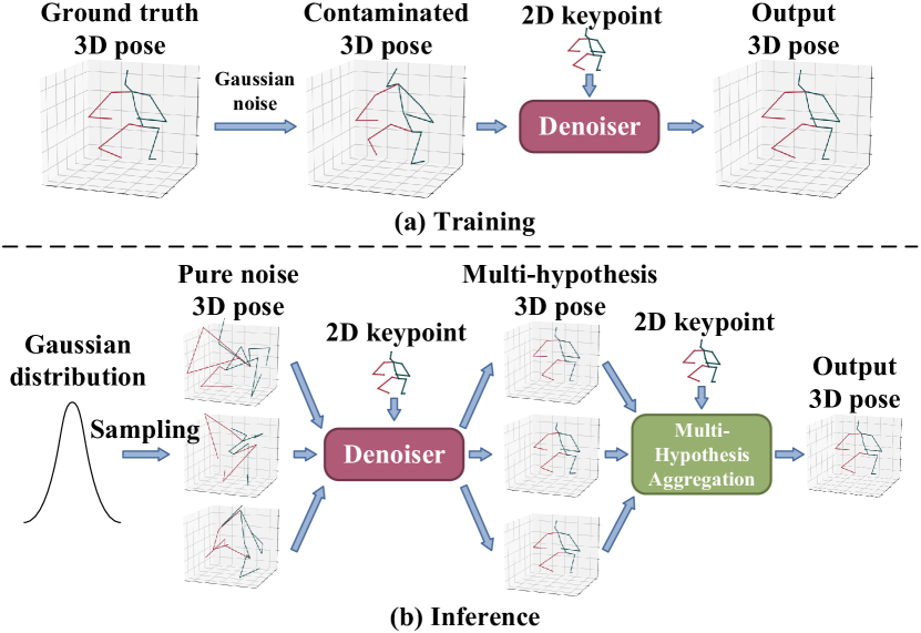
Figure 1: Thumbnail of our D3DP approach with multi-hypothesis aggregation. (a) Training: we gradually destroy the ground truth 3D pose and reverse this process by a denoiser to obtain a clean 3D prediction. (b) Inference: multiple Gaussian noises are passed through the denoiser, which is conditioned on 2D keypoints, to generate plausible 3D pose hypotheses. Then, the proposed multi-hypothesis aggregation method is utilized to yield the final output.

Existing works can be divided into two categories: deterministic and probabilistic approaches. Deterministic approaches [65, 39, 70, 51, 37] are designed to produce a single, definite 3D pose for each image, which is practical in real-world applications. Probabilistic approaches [63, 33, 26, 53, 44] represent the 2D-to-3D lifting as a probability distribution and produce a set of possible solutions for each image, which allows for uncertainty and ambiguity in the lifting process. This paper focuses on probabilistic methods but combines the advantages of deterministic methods, i.e., we aggregate multiple pose hypotheses into a single, higher-quality 3D pose for practical use.

Previous probabilistic approaches use generative models (e.g., generative adversarial networks [19] or normalizing flows [47]) to predict multiple 3D pose hypotheses. Despite the great progress achieved, they still have the following two disadvantages: 1) They either (i) rely on special network designs and have poor compatibility [36, 63, 34, 56], or (ii) cannot specify the number of hypotheses based on actual needs [36, 33, 44]. 2) Although these methods generate multiple possible hypotheses, an individual 3D pose is still needed for practical use. They generally average over multiple hypotheses at the pose level to obtain the final output [53, 33], which does not take into account the differences between joints and the prior distribution of 2D keypoints. Consequently, the averaged result is much worse than the best of all hypotheses.

To address the first problem, we exploit Denoising Diffusion Probabilistic Models (DDPMs) [20] for 3D human pose estimation and introduce a novel approach called Diffusion-based 3D Pose estimation (D3DP). As shown in Fig. 1, our approach involves adding varying levels of noise to the ground truth 3D poses and learning a denoiser to predict the original data during training. During inference, we generate initial 3D poses by sampling pure noise from a Gaussian distribution. These poses are then sent to the denoiser, which is conditioned on 2D keypoints, to predict multiple 3D pose hypotheses. Compared to previous approaches, our method is superior in two aspects. (i) The denoiser has the compatibility to use existing 3D human pose estimators as the backbone, which enables an easy transformation from a deterministic approach into a probabilistic version. (ii) The number of hypotheses can be customized during inference. Besides, the proposed method progressively refines the generated results, which supports an additional adjustable parameter (number of iterations). More hypotheses and iterations bring better results at the expense of greater computational overhead. These two parameters help to strike a balance between performance and efficiency under limited computing resources.

To address the second problem, we focus on how to aggregate multiple 3D pose hypotheses into a single, more accurate 3D prediction. It is observed that the upper-bound performance of aggregation at the joint level is much higher than that at the pose level (Section 4.5), as the former conducts aggregation at a finer granularity. This observation drives us to propose a joint-wise reprojection-based multi-hypothesis aggregation (JPMA) method, which reprojects 3D pose hypotheses back to the 2D camera plane and conducts the joint-level selection of the best hypothesis based on the reprojection errors. The selected joints are assembled into a complete 3D pose as the final output. The proposed method uses joints as granularity, allowing a more diverse combination of hypotheses. In addition, the marginal distribution of 2D keypoints is taken into account, thus aiding the modeling of the posterior distribution of the final 3D pose. Compared to previous methods that use the averaged pose, JPMA integrates joint-level geometric priors into the multi-hypothesis aggregation, and hence improves the prediction performance.

Our contributions can be summarized as follows:

• We propose a diffusion-based 3D human pose estimation (D3DP) method, which is compatible and customizable.

• When multiple hypotheses are combined into a single prediction, we observe that the upper bound of performance for aggregation at the joint level is significantly higher than that at the pose level. This observation drives us to conduct joint-by-joint aggregation. To the best of our knowledge, we are the first to tackle this problem from the joint perspective.

• We propose a joint-wise reprojection-based multi-hypothesis aggregation (JPMA) method, which leverages the 2D prior at the joint level to improve the accuracy of the final 3D prediction. The proposed method proves to be more effective than existing pose-level aggregation methods.

• Our method outperforms both the state-of-the-art deterministic and probabilistic approaches on 3D human pose estimation benchmarks.

2 Related Work

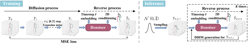
Figure 2: Overview of the proposed D3DP method. Left: Training. $t$-step Gaussian noise is added to the ground truth 3D pose $\bm{y}_{0}$, resulting in the noisy pose $\bm{y}_{t}$. $\bm{y}_{t}$ is then fed to a denoiser conditioned on 2D keypoints $\bm{x}$ and timestep $t$ to yield the final prediction $\widetilde{\bm{y}}_{0}$. Right: Inference. $H$ samples are drawn from a Gaussian distribution to initialize 3D poses $\bm{y}_{0:H,T}$, which are utilized to yield the noiseless 3D pose hypotheses $\widetilde{\bm{y}}_{0:H,0}$. Besides, we can iterate the above reverse process $K$ times to refine the final results by sending DDIM-generated 3D poses $\bm{y}_{0:H,t}$ with different levels of noise to the denoiser.

2.1 Diffusion Model

Diffusion models [55] are a family of generative models that gradually deconstruct observed data by adding noise, and then recover the original data by reversing this process. Denoising Diffusion Probabilistic Models (DDPMs) [20] establish a connection between diffusion models and denoising score matching, which sparks recent interest in this approach. DDPMs have shown remarkable progress in numerous areas, including image generation [21, 41, 3, 48, 49, 50], cross-modal generation [1, 16, 24, 29, 32], graph generation [59, 43, 28, 64], semantic segmentation [2, 5], object detection [8], etc. For example, SR3 [50] adapts DDPMs to super-resolution. DiffusionDet [8] applies diffusion models to object detection to recover bounding boxes from noise. Pix2Seq-D [10] leverages diffusion models based on analog bits for panoptic segmentation.

3D human pose estimation suffers from intrinsic depth ambiguity, making probabilistic generation methods suitable for this task. Since diffusion models are well known for their ability to generate high-fidelity samples, we apply DDPMs to 3D human pose estimation.

2.2 Probabilistic 3D Human Pose Estimation

Early probabilistic methods [54, 31] rely on heuristic approaches to sample multiple plausible 3D poses that could potentially produce similar 2D projections. Recently, approaches based on mixture density networks (MDN) [4], normalizing flows (NF) [47], conditional variational autoencoder (CVAE) [56] and generative adversarial networks (GAN) [19] have been proposed. Li and Lee [33] introduce MDN to generate pose hypotheses, and Oikarinen et al. [44] further combine MDN with graph neural networks that incorporate graph-structured information. Sharma et al. [53] use CVAE to obtain diverse 3D pose samples. Wehrbein et al. [63] and Li et al. [34] exploit NF and GAN for this task, respectively. Besides, MHFormer [36] uses a Transformer [58] to generate three features to represent three individual hypotheses.

To overcome the drawbacks of previous methods, such as bad compatibility (MHFormer, NF, GAN, MDN, CVAE), and a non-adjustable number of hypotheses (MHFormer, MDN), we present D3DP, a straightforward and compatible architecture that can be easily integrated with existing 3D pose estimators with minimal modifications. Our method supports a custom number of iterations $K$ and hypotheses $H$ during inference to balance performance and efficiency. Note that concurrent methods [22, 18, 14] also use diffusion models for this task, but they either don’t use any aggregation method or use a pose-level method (average). In contrast, we propose a joint-level aggregation method, called JPMA, to achieve a more accurate prediction.

2.3 Multi-Hypothesis Aggregation

Probabilistic 3D pose estimation methods typically generate multiple hypotheses, but how to synthesize them into a single 3D pose is still an open research question. Many methods [63, 33, 44, 34] simply average all pose hypotheses, which often produces unsatisfactory results. Other approaches explore more sophisticated ways of aggregating multiple hypotheses. Sharma et al. [53] use depth ordinal relations to score and weight-average the candidate 3D poses. Oikarinen et al. [44] choose the 3D pose with the highest mixture coefficient outputted by MDN. However, these works ignore the differences between joints. Besides, the information contained in 2D keypoints is not exploited.

Thus, our JPMA method is proposed to use the errors between the reprojected hypotheses and the input 2D keypoints as guidance for joint-level hypothesis selection. Although other approaches [46, 61, 12, 7, 30] have already used the 3D-to-2D reprojection method in deterministic 3D human pose estimation, our method marks the pioneering effort to apply it to probabilistic estimation. Specifically, reprojection is incorporated into the multi-hypothesis aggregation (MHA), which provides a new perspective on this problem.

3 Method

Given the input 2D keypoints $\bm{x}=\{p^{\text{2d}}_{n}\}_{n=0}^{N},p^{\text{2d}}_{n}\in\mathbb{R}^{J\times 2}$, our goal is to predict the corresponding 3D positions of all joints $\widetilde{\bm{y}}=\{p^{\text{3d}}_{n}\}_{n=0}^{N},p^{\text{3d}}_{n}\in\mathbb{R}^{J\times 3}$. $N,J$ are the number of frames and human joints in each frame, respectively. Since diffusion models can generate high-quality samples, we apply it to probabilistic 3D human pose estimation and propose D3DP method, which generates multiple 3D pose hypotheses for a single 2D observation. Then, these hypotheses are used by the proposed JPMA method to yield a single, accurate 3D pose for practical use.

3.1 Diffusion-Based 3D Pose Estimation (D3DP)

D3DP uses two Markov chains: 1) a diffusion process that gradually perturbs data to noise, and 2) a reverse process that reconstructs the uncontaminated data by a denoiser. For more information about diffusion models, please refer to Appendix A. The training and inference phases of D3DP are described in detail below.

Training.

As shown in Fig. 2 (left), we first sample a timestep $t\sim U(0,T)$, where $T$ is the maximum number of timesteps. Then the ground truth 3D pose $\bm{y}_{0}$ is diffused to the corrupted pose $\bm{y}_{t}$ by adding $t$-step independent Gaussian noise $\epsilon\sim\mathcal{N}(0,\bm{I})$. Following DDPMs [20], this process can be formulated as

$$\begin{split}q(\bm{y}_{t}\mid\bm{y}_{0})&\coloneqq\sqrt{\bar{\alpha}_{t}}\bm{y}_{0}+\epsilon\sqrt{1-\bar{\alpha}_{t}}\end{split}$$ (1)

where $\bar{\alpha}_{t}\coloneqq\prod_{s=0}^{t}\alpha_{s}$ and $\alpha_{t}\coloneqq 1-\beta_{t}$. $\beta_{t}$ is the cosine noise variance schedule. When $T$ is large enough, the distribution of $q(\bm{y}_{T})$ is nearly an isotropic Gaussian distribution.

Subsequently, $\bm{y}_{t}$ is sent to a denoiser $\mathfrak{D}$ conditioned on 2D keypoints $\bm{x}$ and timestep $t$ to reconstruct the 3D pose $\widetilde{\bm{y}}_{0}$ without noise:

$$\begin{split}\widetilde{\bm{y}}_{0}=\mathfrak{D}\left(\bm{y}_{t},\bm{x},t\right)\end{split}$$ (2)

The entire framework is supervised by a simple MSE loss:

$$\begin{split}\mathcal{L}=||\bm{y}_{0}-\widetilde{\bm{y}}_{0}||_{2}\end{split}$$ (3)

Inference.

Since the degraded data is well approximated by a Gaussian distribution after the diffusion process, we can obtain $H$ initial 3D poses $\bm{y}_{0:H,T}$ by sampling noise from a unit Gaussian. As shown in Fig. 2 (right), feasible 3D pose hypotheses $\widetilde{\bm{y}}_{0:H,0}$ are predicted by passing $\bm{y}_{0:H,T}$ to the denoiser $\mathfrak{D}$ (Eq. 2).

Thereafter, $\widetilde{\bm{y}}_{0:H,0}$ are used to generate the noisy 3D poses $\widetilde{\bm{y}}_{0:H,t^{\prime}}$ as inputs to the denoiser for the next timestep via DDIM [57], which can be formulated as

$$\begin{split}\bm{y}_{0:H,t^{\prime}}=\sqrt{\bar{\alpha}_{t^{\prime}}}\cdot\widetilde{\bm{y}}_{0:H,0}+\sqrt{1-\bar{\alpha}_{t^{\prime}}-\sigma_{t}^{2}}\cdot\epsilon_{t}+\sigma_{t}\epsilon\end{split}$$ (4)

where $t,t^{\prime}$ are the current and next timesteps, respectively. The initial $t=T$. $\epsilon\sim\mathcal{N}(0,\bm{I})$ is standard Gaussian noise independent of $\bm{y}_{0:H,t}$ and

$$\begin{split}\epsilon_{t}&=\left(\bm{y}_{0:H,t}-\sqrt{\bar{\alpha}_{t}}\cdot\widetilde{\bm{y}}_{0:H,0}\right)/\sqrt{1-\bar{\alpha}_{t}}\\ \sigma_{t}&=\sqrt{\left(1-\bar{\alpha}_{t^{\prime}}\right)/\left(1-\bar{\alpha}_{t}\right)}\cdot\sqrt{1-\bar{\alpha}_{t}/\bar{\alpha}_{t^{\prime}}}\end{split}$$ (5)

where $\epsilon_{t}$ is the noise at timestep $t$ (derived from Eq. 1). $\sigma_{t}$ controls how stochastic the diffusion process is.

Then, we can regenerate $\widetilde{\bm{y}}_{0:H,0}$ using $\bm{y}_{0:H,t^{\prime}}$ as inputs to the denoiser. This procedure will be iterated $K$ times. Since we start from T at the beginning, the timestep of each iteration can be written as $t=T\cdot\left(1-k/K\right),k\in[0,K)$. The detailed algorithm is provided in Appendix C.

In this way, the proposed method supports a customizable number of hypotheses $H$ by sampling multiple times from a Gaussian distribution. Moreover, the denoiser is trained only once but can be used multiple times to progressively refine the final predictions during inference. This refinement process supports an additional adjustable parameter (number of iterations $K$), which controls the diversity and quality of the generated hypotheses. Thus, we can specify an arbitrary number of $H,K$ during inference (both are set to 1 during training), which allows users to balance performance and efficiency. This property solves the problem of a non-adjustable number of hypotheses faced by previous methods [36, 33, 44].

3.2 Joint-Wise Reprojection-Based
Multi-Hypothesis Aggregation (JPMA)

Previous probabilistic 3D pose estimation methods [26, 47, 33] mainly focus on the generation of 3D pose hypotheses, with little attention to how to aggregate multiple hypotheses to produce a single, high-fidelity prediction. These approaches typically report the error of the best 3D pose (i.e., closest to the ground truth) to highlight the superiority of their methods. However, this metric only demonstrates the upper bound of the performance and is not feasible in real-world applications because the ground truth is not available. Therefore, the averaged 3D pose is used as the final prediction, while its performance is far worse than the best result. A few works [44, 53] explore multi-hypothesis aggregation methods that are more effective than average for testing on in-the-wild videos. However, they use poses as granularity and ignore the distinctions between joints. Also, they do not establish the correspondence between 3D predictions and the 2D observation. Hence, further improvements are needed to achieve more accurate and reliable results.

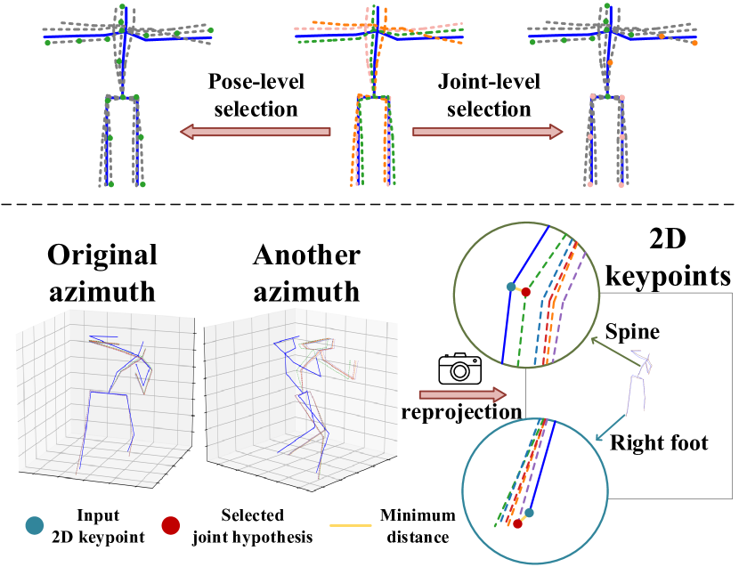
Figure 3: Top: Comparison between the pose-level (existing methods) and joint-level (proposed method) selections. The selected joint is drawn in the color of the hypothesis it belongs to. Bottom: Our JPMA method. 3D pose hypotheses are reprojected to the 2D camera plane and compared with the input 2D keypoints. For each joint, we select the best hypothesis that has the minimum distance to the 2D input. Dashed line: predicted 3D pose hypotheses. Each color represents an individual hypothesis. Solid blue line: ground truth 3D poses.

To alleviate these problems, we first validate the upper-bound performance of aggregation methods at two levels by choosing the best hypothesis that is closest to the ground truth. In the case of pose level, the best pose is selected as the final prediction. In the case of joint level, the best joint is selected and all the selected joints are combined into the final prediction. Experimental results show that the latter has a higher upper-bound performance than the former (Section 4.5), as the joint-level aggregation allows more flexible combinations of hypotheses. An intuitive comparison between the upper bounds of joint-level and pose-level selections (aggregations) is shown in Fig. 3 (top). When the pose-level selection is used, the green hypothesis (best pose) will be used as the results for all joints. However, the performance of the same hypothesis may vary across joints. Thus, the joint-level selection decomposes and recombines the hypotheses at the joint level instead of viewing each 3D pose as a whole. Only a fraction of joints (those with better performance) in each hypothesis will be used by the joint-level selection, and then these selected joints are assembled into an independent 3D pose. In this way, the advantage of each hypothesis is maximized. Moreover, the input 2D keypoints can be used as geometric priors to guide the model to choose the most likely 3D pose $\widetilde{\bm{y}}_{0}$ with the maximum posterior probability $q(\widetilde{\bm{y}}_{0}|\bm{x},\widetilde{\bm{y}}_{0:H,0})$ as the final prediction during inference. Although 2D keypoints contain no depth information about 3D poses, they indicate the possible locations of human joints in 3D space (i.e., the joint should be on the ray from the camera’s optical center to the 2D keypoint). Thus, 2D keypoints still play an important role in multi-hypothesis aggregation.

Based on the above two ideas, we propose a joint-wise reprojection-based multi-hypothesis aggregation (JPMA) method, which is illustrated in Fig. 3 (bottom). We use known or estimated intrinsic camera parameters (4 for pinhole camera and 9 for distorted pinhole camera) to reproject 3D hypotheses $\widetilde{\bm{y}}_{0:H,0}$ to the 2D camera plane. Then, we calculate the distance between each hypothesis and the input 2D keypoint $\bm{x}$ for each joint, and select the joint hypothesis with the minimum distance (reprojection error). This process allows us to choose distinct hypotheses for different joints (green hypothesis for the spine and purple hypothesis for the right foot) and combine all the selected joints into the final prediction $\widetilde{\bm{y}}_{0}$, which can be formulated as:

$$\begin{split}\widetilde{\bm{y}}_{0}^{(i)}=\widetilde{\bm{y}}_{h^{\prime},0}^{(i)},\quad h^{\prime}=\underset{h\in[0,H]}{\arg\min}||\mathcal{P}\left(\widetilde{\bm{y}}_{h,0}^{(i)}\right)-\bm{x}^{(i)}||_{2}\end{split}$$ (6)

where $i$ is the index of joints. $\mathcal{P}(\cdot)$ is the reprojection function, which is detailed in Appendix B.

3.3 Architecture

The previous approaches [63, 36, 34, 56] rely on special network designs, for example, MHFormer [36] needs to use the cross-hypothesis interaction module and NF [63] requires the construction of bijective transformations. Therefore, they cannot keep up with the latest 3D human pose estimation methods. While the proposed D3DP method is compatible with up-to-date deterministic 3D pose estimators by using them as the backbone of the denoiser. In this paper, we use MixSTE [68], a mixed spatial temporal Transformer-based method, as the backbone. We can easily transform a deterministic pose estimation approach into a probabilistic version by making minor modifications, which are introduced in the next two paragraphs.

2D conditioning.

Since our goal is to estimate 3D poses from 2D keypoints, using only noisy 3D poses $\bm{y}_{0:H,t}$ as inputs to the denoiser is not sufficient. Therefore, 2D keypoints $\bm{x}$ are used as additional information to guide the denoising process. We implement several schemes for fusing 2D keypoints and noisy 3D poses, such as cross attention, concatenation, etc. According to the experimental results (Appendix D.1), we choose to directly concatenate $\bm{x}$ and $\bm{y}_{0:H,t}$, and send them to the denoiser as inputs.

Timestep embedding.

As the denoiser needs to handle 3D poses with different levels of noise, it is necessary to provide information about the current timestep $t$, which represents the number of times the Gaussian noise is added. Following DDPMs, we use a sinusoidal function to transform $t$ into a timestep embedding and add it after the input embedding in the same way as the Transformer positional embedding [58].

These two modifications bring a negligible amount of computation. In addition, JPMA mainly consists of a reprojection process (without network parameters), so its amount of computation can also be ignored. Therefore, the computational overhead of the proposed D3DP with JPMA (when $H$=$K$=1) is essentially the same as that of the backbone network.

Deterministic Methods
MPJPE		Dir.	Disc.	Eat	Greet	Phone	Photo	Pose	Pur.	Sit	SitD.	Smoke	Wait	WalkD.	Walk	WalkT.	Avg
TCN [46] ($N$=243)*	CVPR’19	45.2	46.7	43.3	45.6	48.1	55.1	44.6	44.3	57.3	65.8	47.1	44.0	49.0	32.8	33.9	46.8
SRNet [65] ($N$=243)*	ECCV’20	46.6	47.1	43.9	41.6	45.8	49.6	46.5	40.0	53.4	61.1	46.1	42.6	43.1	31.5	32.6	44.8
PoseFormer [70] ($N$=81)*	ICCV’21	41.5	44.8	39.8	42.5	46.5	51.6	42.1	42.0	53.3	60.7	45.5	43.3	46.1	31.8	32.2	44.3
RIE [52] ($N$=243)*	MM’21	40.8	44.5	41.4	42.7	46.3	55.6	41.8	41.9	53.7	60.8	45.0	41.5	44.8	30.8	31.9	44.3
Anatomy [9] ($N$=243)*	TCSVT’21	41.4	43.5	40.1	42.9	46.6	51.9	41.7	42.3	53.9	60.2	45.4	41.7	46.0	31.5	32.7	44.1
U-CDGCN [23] ($N$=96)*	MM’21	38.0	43.3	39.1	39.4	45.8	53.6	41.4	41.4	55.5	61.9	44.6	41.9	44.5	31.6	29.4	43.4
Ray3D [66] ($N$=9)*	CVPR’22	44.7	48.7	48.7	48.4	51.0	59.9	46.8	46.9	58.7	61.7	50.2	46.4	51.5	38.6	41.8	49.7
STE [35] ($N$=351)*	TMM’22	39.9	43.4	40.0	40.9	46.4	50.6	42.1	39.8	55.8	61.6	44.9	43.3	44.9	29.9	30.3	43.6
P-STMO [51] ($N$=243)*	ECCV’22	38.9	42.7	40.4	41.1	45.6	49.7	40.9	39.9	55.5	59.4	44.9	42.2	42.7	29.4	29.4	42.8
MixSTE [68] ($N$=243)*$\ddagger$	CVPR’22	37.9	40.1	37.5	39.4	43.3	50.0	39.8	39.9	52.5	56.6	42.4	40.1	40.5	27.6	27.7	41.0
MixSTE [68] ($N$=243)*	CVPR’22	37.6	40.9	37.3	39.7	42.3	49.9	40.1	39.8	51.7	55.0	42.1	39.8	41.0	27.9	27.9	40.9
DUE [67] ($N$=300)*	MM’22	37.9	41.9	36.8	39.5	40.8	49.2	40.1	40.7	47.9	53.3	40.2	41.1	40.3	30.8	28.6	40.6
bestcolorD3DP ($N$=243, $H$=1, $K$=1)*	bestcolor	bestcolor37.7	bestcolor39.9	bestcolor35.7	bestcolor38.2	bestcolor41.9	bestcolor48.8	bestcolor39.5	bestcolor38.3	bestcolor50.5	bestcolor53.9	bestcolor41.6	bestcolor39.4	bestcolor39.8	bestcolor27.4	bestcolor27.5	bestcolor40.0
Probabilistic Methods
MPJPE		Dir.	Disc.	Eat	Greet	Phone	Photo	Pose	Pur.	Sit	SitD.	Smoke	Wait	WalkD.	Walk	WalkT.	Avg
CVAE [53] ($N$=1, $H$=200, P-Agg)	ICCV’19	48.6	54.5	54.2	55.7	62.6	72.0	50.5	54.3	70.0	78.3	58.1	55.4	61.4	45.2	49.7	58.0
GAN [34] ($N$=1, $H$=10, P-Agg)	BMVC’20	67.9	75.5	71.8	81.8	81.4	93.7	75.2	81.3	88.8	114.1	75.9	79.1	83.3	74.3	79.0	81.1
GraphMDN [44] ($N$=1, $H$=5, P-Agg)	IJCNN’21	51.9	56.1	55.3	58.0	63.5	75.1	53.3	56.5	69.4	92.7	60.1	58.0	65.5	49.8	53.6	61.3
NF [63] ($N$=1, $H$=1, P-Agg)	ICCV’21	52.4	60.2	57.8	57.4	65.7	74.1	56.2	59.1	69.3	78.0	61.2	63.7	67.0	50.0	54.9	61.8
MHFormer [36] ($N$=351, $H$=3, P-Agg)*	CVPR’22	39.2	43.1	40.1	40.9	44.9	51.2	40.6	41.3	53.5	60.3	43.7	41.1	43.8	29.8	30.6	43.0
bestcolorD3DP ($N$=243, $H$=1, $K$=1, P-Agg)*	bestcolor	bestcolor37.7	bestcolor39.9	bestcolor35.7	bestcolor38.2	bestcolor41.9	bestcolor48.8	bestcolor39.5	bestcolor38.3	bestcolor50.5	bestcolor53.9	bestcolor41.6	bestcolor39.4	bestcolor39.8	bestcolor27.4	bestcolor27.5	bestcolor40.0
bestcolorD3DP ($N$=243, $H$=20, $K$=10, P-Agg)*	bestcolor	bestcolor37.6	bestcolor39.7	bestcolor35.8	bestcolor38.0	bestcolor41.7	bestcolor48.7	bestcolor39.4	bestcolor38.2	bestcolor50.3	bestcolor53.3	bestcolor41.4	bestcolor39.4	bestcolor39.7	bestcolor27.4	bestcolor27.3	bestcolor39.9
bestcolorD3DP ($N$=243, $H$=20, $K$=10, J-Agg)*	bestcolor	bestcolor37.3	bestcolor39.5	bestcolor35.6	bestcolor37.8	bestcolor41.3	bestcolor48.2	bestcolor39.1	bestcolor37.6	bestcolor49.9	bestcolor52.8	bestcolor41.2	bestcolor39.2	bestcolor39.4	bestcolor27.2	bestcolor27.1	bestcolor39.5
MDN [33] ($N$=1, $H$=5, P-Best$\sharp$)	CVPR’19	43.8	48.6	49.1	49.8	57.6	64.5	45.9	48.3	62.0	73.4	54.8	50.6	56.0	43.4	45.5	52.7
CVAE [53] ($N$=1, $H$=200, P-Best$\sharp$)	ICCV’19	37.8	43.2	43.0	44.3	51.1	57.0	39.7	43.0	56.3	64.0	48.1	45.4	50.4	37.9	39.9	46.8
GAN [34] ($N$=1, $H$=10, P-Best$\sharp$)	BMVC’20	62.0	69.7	64.3	73.6	75.1	84.8	68.7	75.0	81.2	104.3	70.2	72.0	75.0	67.0	69.0	73.9
GraphMDN [44] ($N$=1, $H$=200, P-Best$\sharp$)	IJCNN’21	40.0	43.2	41.0	43.4	50.0	53.6	40.1	41.4	52.6	67.3	48.1	44.2	49.0	39.5	40.2	46.2
NF [63] ($N$=1, $H$=200, P-Best$\sharp$)	ICCV’21	38.5	42.5	39.9	41.7	46.5	51.6	39.9	40.8	49.5	56.8	45.3	46.4	46.8	37.8	40.4	44.3
bestcolorD3DP ($N$=243, $H$=1, $K$=1, P-Best$\sharp$)*	bestcolor	bestcolor37.7	bestcolor39.9	bestcolor35.7	bestcolor38.2	bestcolor41.9	bestcolor48.8	bestcolor39.5	bestcolor38.3	bestcolor50.5	bestcolor53.9	bestcolor41.6	bestcolor39.4	bestcolor39.8	bestcolor27.4	bestcolor27.5	bestcolor40.0
bestcolorD3DP ($N$=243, $H$=20, $K$=10, P-Best$\sharp$)*	bestcolor	bestcolor37.3	bestcolor39.4	bestcolor35.4	bestcolor37.8	bestcolor41.3	bestcolor48.1	bestcolor39.0	bestcolor37.9	bestcolor49.8	bestcolor52.8	bestcolor41.1	bestcolor39.0	bestcolor39.4	bestcolor27.3	bestcolor27.2	bestcolor39.5
bestcolorD3DP ($N$=243, $H$=20, $K$=10, J-Best$\sharp$)*	bestcolor	bestcolor33.0	bestcolor34.8	bestcolor31.7	bestcolor33.1	bestcolor37.5	bestcolor43.7	bestcolor34.8	bestcolor33.6	bestcolor45.7	bestcolor47.8	bestcolor37.0	bestcolor35.0	bestcolor35.0	bestcolor24.3	bestcolor24.1	bestcolor35.4

Table 1: Results on Human3.6M in millimeters under MPJPE. $N,H,K$: the number of input frames, hypotheses, and iterations of the proposed D3DP. ($\ddagger$) - Our implementation. ($\sharp$) - Not feasible in real-world applications. (*) - Use CPN  [11] as the 2D keypoint detector to generate the inputs. Red: Best. Blue: Second best. Gray: our method.

4 Experiments

4.1 Datasets and Evaluation Metrics

Human3.6M (H36M)

[25] is the largest and most commonly used indoor dataset. It contains 15 activities (e.g., walking) performed by 11 actors. Videos are captured by 4 synchronized and calibrated cameras at 50Hz. Following [36, 46, 44], our model is trained on 5 subjects (S1, S5, S6, S7, S8) and evaluated on 2 subjects (S9, S11). For evaluation metrics, we report the mean per joint position error (MPJPE), which computes the mean Euclidean distance between estimated and ground truth 3D joint positions in millimeters. Besides, Procrustes MPJPE (P-MPJPE) is also reported, which computes MPJPE after the estimated poses align to the ground truth using a rigid transformation.

MPI-INF-3DHP (3DHP)

[40] is a recently popular dataset consisting of indoor and outdoor scenes. The training set contains 8 activities performed by 8 actors, and the test set covers 7 activities. Following [51], we use the valid frames provided by the official for testing. For evaluation metrics, we report MPJPE, percentage of correct keypoint (PCK) within 150mm range, and area under curve (AUC).

3DPW

[60] is the first dataset in the wild that includes video footage taken from a moving phone camera. We train our method on Human3.6M and evaluate on this dataset to show the qualitative results.

4.2 Implementation Details

We use MixSTE [68] as the backbone of the denoiser, which makes use of factorized attention by combining multiple spatial and temporal attention layers. It contains 16 alternating spatial and temporal Transformer layers [58] with the channel size set to 512. We modify MixSTE to fit the diffusion framework as follows: concatenating 2D keypoints and noisy 3D poses as inputs; adding timestep embedding after the input embedding in the first layer. The detailed architecture of the denoiser is shown in Fig. 4.

The proposed method is implemented in PyTorch [45] using AdamW [38] optimizer with the momentum parameters as $\beta_{1},\beta_{2}=0.9,0.999$ and the weight decay as 0.1. We train our model for 400 epochs and the initial learning rate is $6e^{-5}$ with a shrink factor of 0.993 after each epoch. We set the batch size to 4 and each sample contains a pose sequence of 243 frames ($N$=243). During training, the number of hypotheses and iterations $H,K$ are set to 1,1, respectively. During inference, they are set to 20, 10. The maximum number of timesteps $T$ is set to 1000. All experiments are carried out on two GeForce RTX 3080 Ti GPUs.

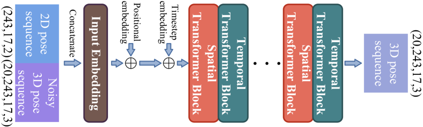
Figure 4: Detailed architecture of the denoiser. The tensor sizes are shown in parentheses. The 2D pose sequence (243,17,2) is expanded, repeated, and then concatenated with the noisy 3D pose sequence (20,243,17,3) to get the input sequence (20,243,17,5). 20, 243, 17 are the number of hypotheses $H$, frames $N$, and human joints $J$ in each frame, respectively.

H36M		3DHP		3DPW

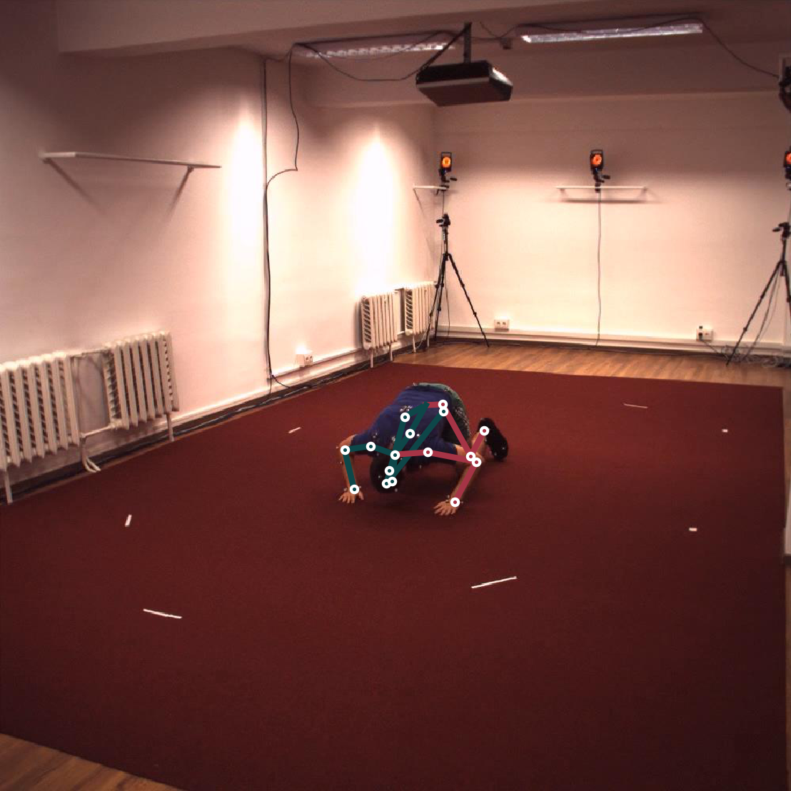
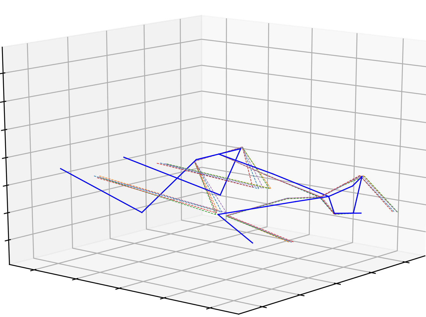
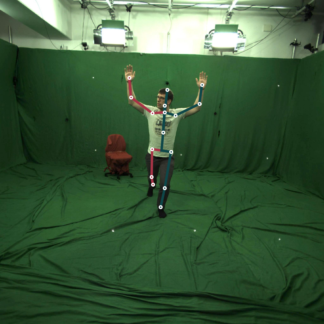
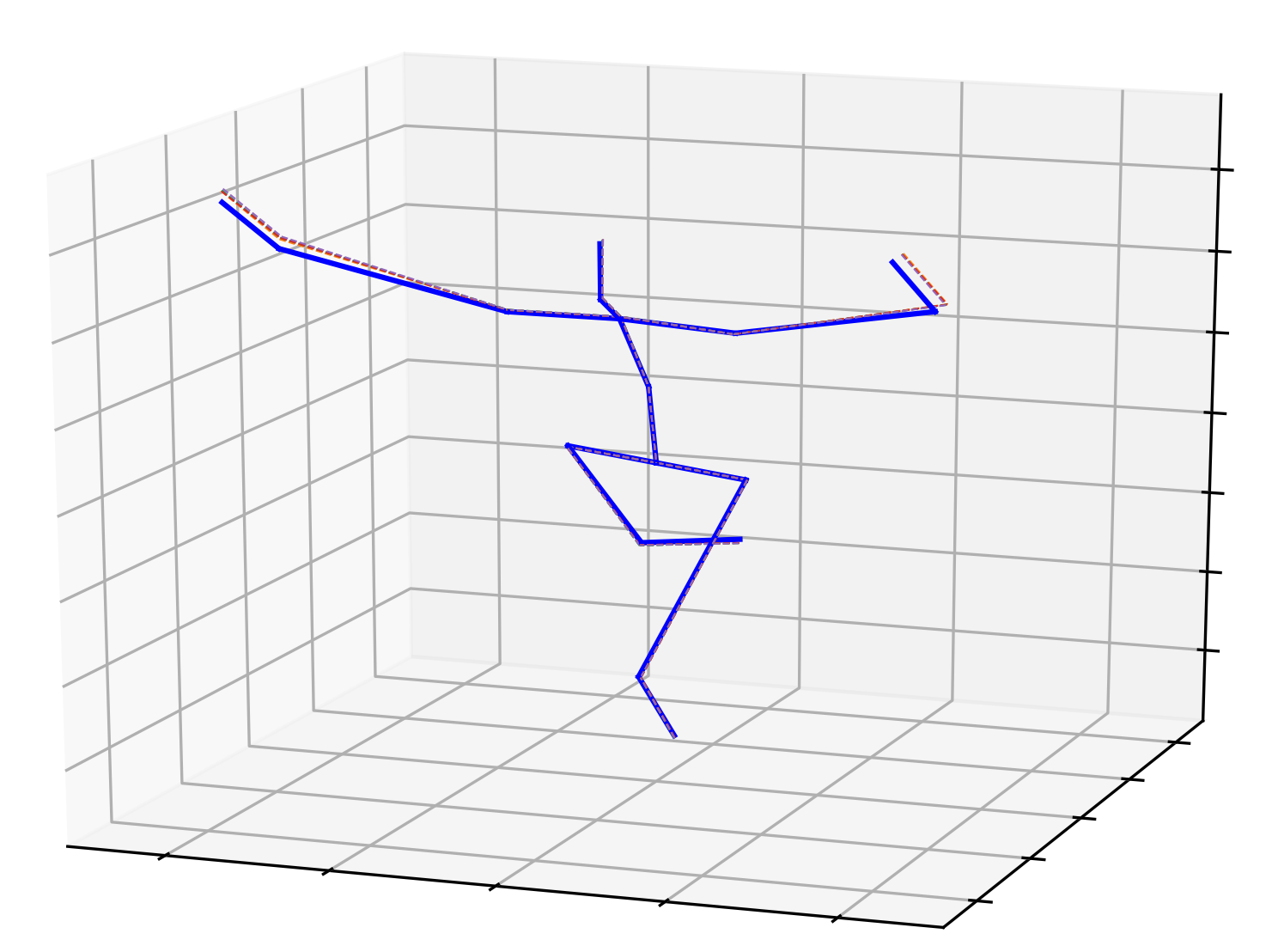
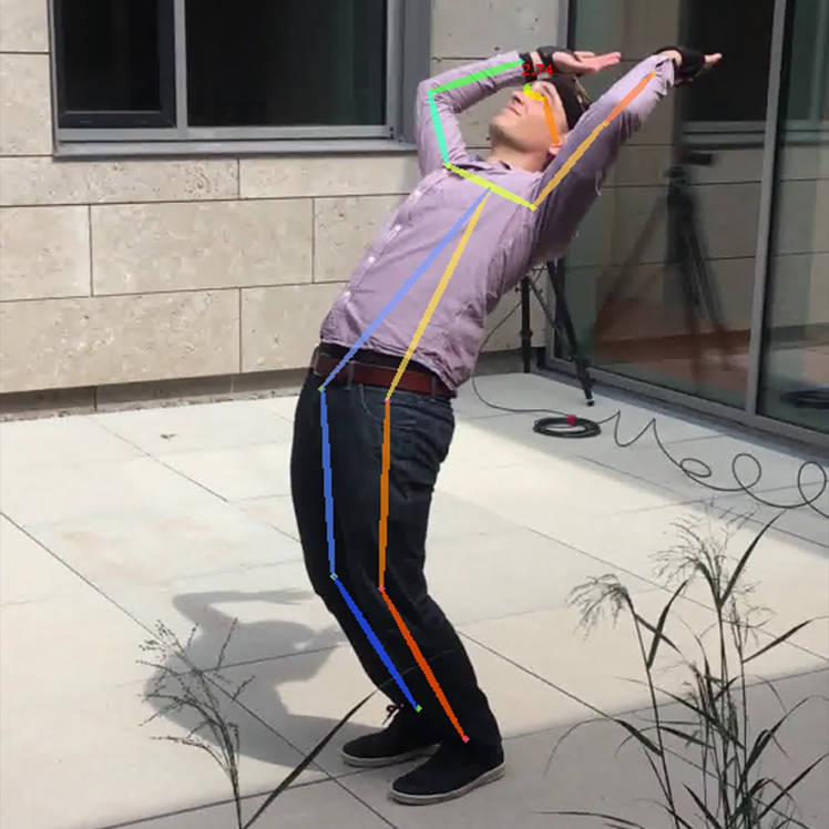
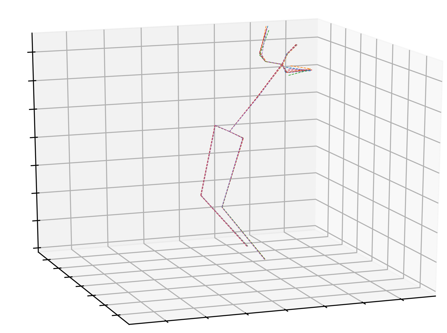
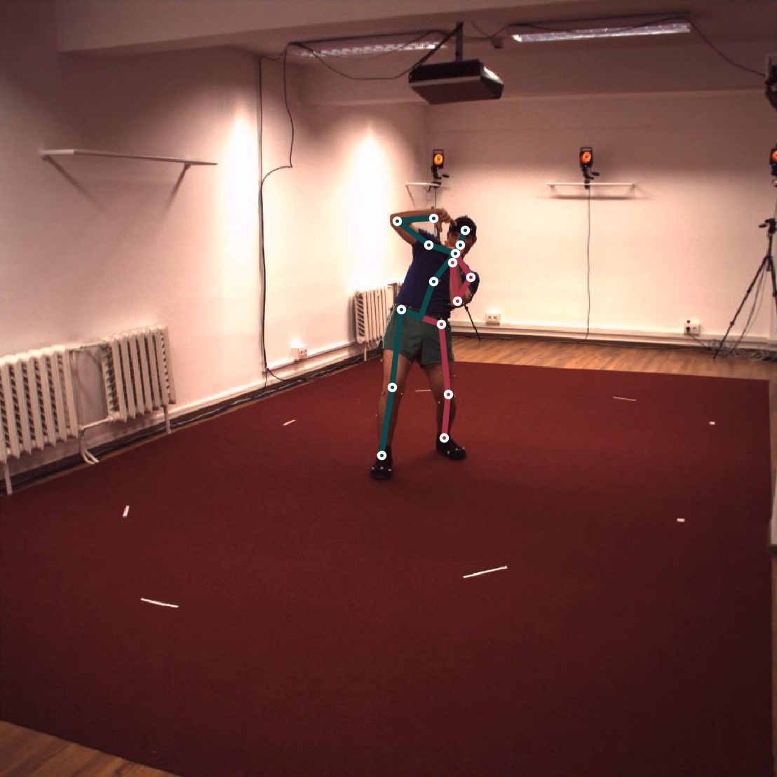
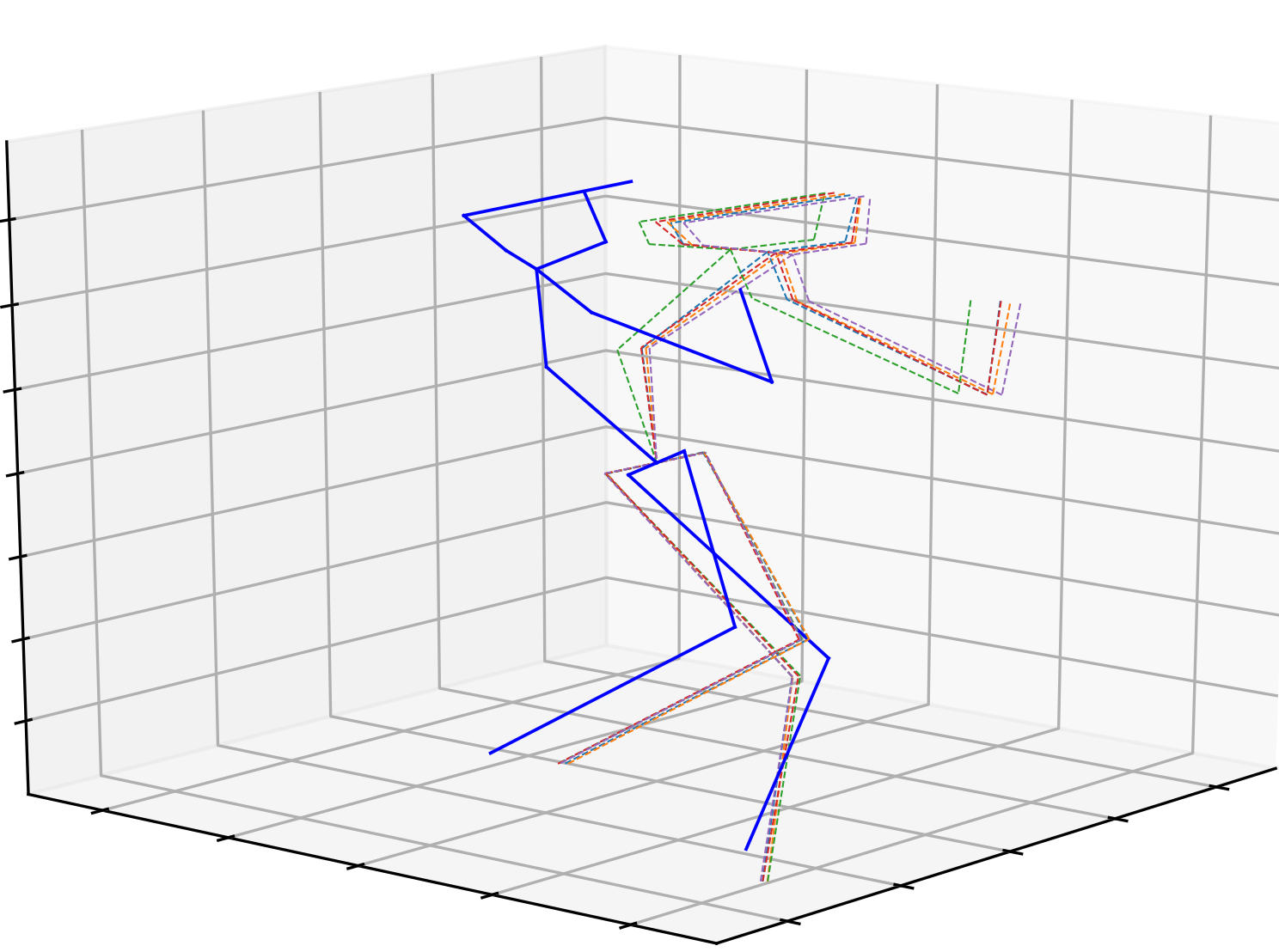
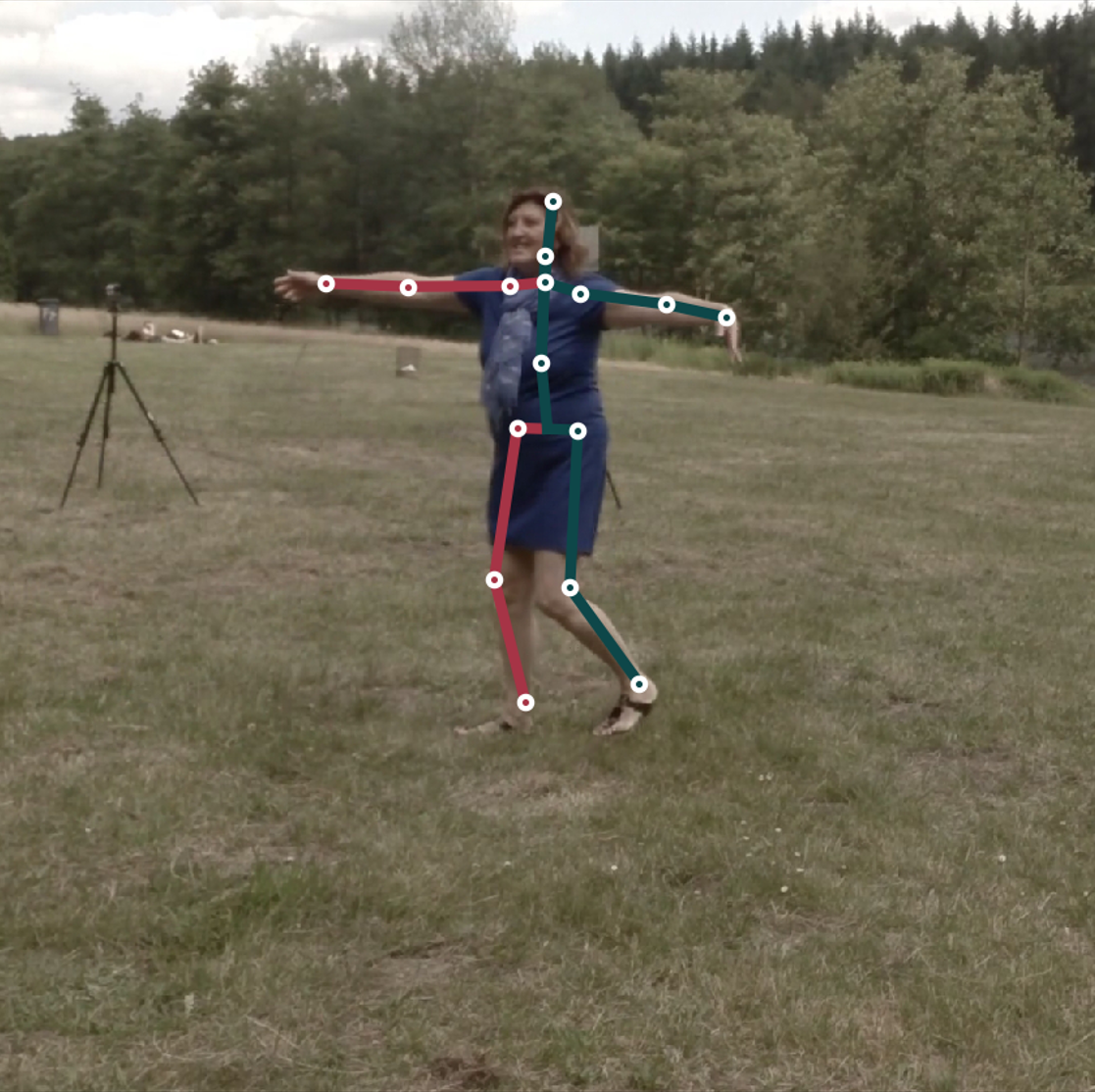
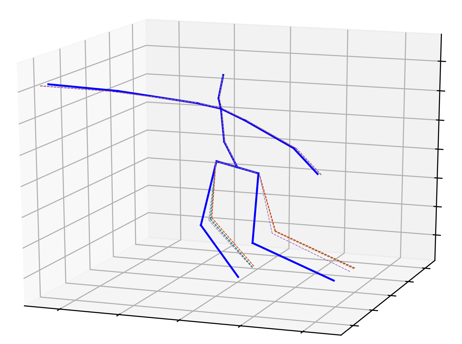
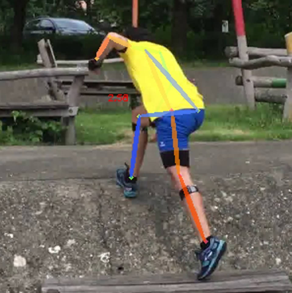
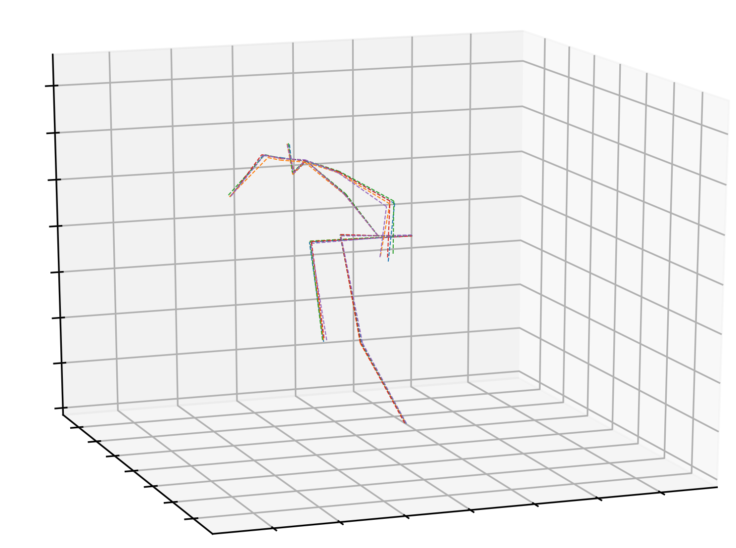
Figure 5: Qualitative results on three datasets. Dashed line: predicted 3D pose hypotheses. Each color represents an individual hypothesis. Solid blue line: ground truth 3D poses.

4.3 Quantitative Results

Human3.6M.

As shown in Table 1 (top), we compare the proposed D3DP with the state-of-the-art deterministic 3D human pose estimation methods on Human3.6M. For fairness, we set $H$=1 to produce a single prediction. Our D3DP ($N$=243) achieves 40.0mm under MPJPE, outperforming DUE [67] ($N$=300) by 0.6mm, even though we use fewer frames. Moreover, our method exceeds MixSTE [68] (our backbone) by 1 mm under MPJPE. Although our method aims to generate multiple 3D pose hypotheses, it still improves performance in the single-hypothesis case. This result demonstrates that D3DP (i.e., conditional denoising from corrupted 3D poses) helps the network generalize better to the test set, thus improving the prediction accuracy.

Additionally, D3DP is compared with other probabilistic methods, as shown in Table 1 (bottom). We report the results according to the following four experimental settings.

• P-Agg: Use pose-level aggregation methods, which treat each 3D pose as the smallest unit to compose the final prediction, such as depth ordinal guidance [53], mean [44] and mean-shift [34].

• J-Agg (proposed): Use joint-level aggregation methods (our JPMA) to yield the final prediction. Each joint is treated as the smallest unit.

• P-Best$\sharp$: Select the 3D pose hypothesis that is closest to the ground truth. It is the upper bound of P-Agg performance.

• J-Best$\sharp$ (proposed): Select the joint hypothesis that is closest to the ground truth, and then combine the selected joints into the final 3D pose. It is the upper bound of J-Agg performance.

($\sharp$) refers to the settings that are not feasible for in-the-wild videos. When testing under traditional P-Best and P-Agg (average is used in our experiments), our approach has a significant improvement over NF [63] (4.8mm) and MHFormer [36] (3.1mm), respectively. However, the increase of $H$ (1$\rightarrow$20) does not significantly improve the performance of the proposed D3DP method under P-Best (40.0$\rightarrow$39.5mm). This result prompts us to propose the new setting J-best, under which a noticeable improvement (40.0$\rightarrow$35.4mm) can be observed. It is because the same hypothesis may perform differently depending on which joint is being considered. This observation motivates us to propose J-Agg (using our JPMA) to exploit the joint-level differences between hypotheses. Compared to P-Agg, the performance under J-Agg is boosted (39.9$\rightarrow$39.5mm). This performance is the same as P-Best (39.5mm). More results in terms of P-MPJPE or using 2D ground truth as inputs are provided in Appendix E.

Method		PCK$\uparrow$	AUC$\uparrow$	MPJPE$\downarrow$
U-CDGCN [23] ($N$=96)$\triangledown$	MM’21	97.9	69.5	42.5
P-STMO [51] ($N$=81)$\triangledown$	ECCV’22	97.9	75.8	32.2
TCN [46] ($N$=81)	CVPR’19	86.0	51.9	84.0
U-GCN [62] ($N$=96)	ECCV’20	86.9	62.1	68.1
Anatomy [9] ($N$=81)	TCSVT’21	87.9	54.0	78.8
PoseFormer [70] ($N$=9)	ICCV’21	88.6	56.4	77.1
MHFormer [36] ($N$=9, $H$=3, P-Agg)	CVPR’22	93.8	63.3	58.0
MixSTE [68] ($N$=27)	CVPR’22	94.4	66.5	54.9
MixSTE [68] ($N$=243)$\ddagger$	CVPR’22	96.9	75.8	35.4
bestcolorD3DP ($N$=243, $H$=1, $K$=1)	bestcolor	bestcolor97.7	bestcolor77.8	bestcolor30.2
bestcolorD3DP ($N$=243, $H$=20, $K$=20, P-Agg)	bestcolor	bestcolor97.7	bestcolor78.0	bestcolor30.0
bestcolorD3DP ($N$=243, $H$=20, $K$=20, J-Agg)	bestcolor	bestcolor97.7	bestcolor78.2	bestcolor29.7
bestcolorD3DP ($N$=243, $H$=20, $K$=20, P-Best$\sharp$)	bestcolor	bestcolor97.8	bestcolor78.2	bestcolor29.8
bestcolorD3DP ($N$=243, $H$=20, $K$=20, J-Best$\sharp$)	bestcolor	bestcolor98.0	bestcolor79.1	bestcolor28.1

Table 2: Results on MPI-INF-3DHP under three evaluation metrics using ground truth 2D keypoints as inputs. ($\triangledown$) - They train and evaluate on 3D poses scaled to the height of the universal skeleton used by H36M, while we use the ground truth 3D poses.

MPI-INF-3DHP.

Table 2 shows comparisons between our method and others on 3DHP dataset. D3DP reduces the MPJPE by 5.2mm on top of MixSTE [68] in the single-hypothesis case ($H$=1). When $H$ is increased to 20, the performance under J-Agg using JPMA is similar to P-Best and superior to P-Agg. Our method performs best when evaluated under J-Best. These results exhibit the same pattern as those on Human3.6M, which demonstrates the strong generalization capability of our method.

4.4 Qualitative Results

Fig. 5 shows the qualitative results of D3DP on three datasets with $H,K$ set to 5. For the cases of 2D keypoint misdetection (top left: right knee), occlusion (top left: lower body, bottom right: right arm), and depth ambiguity (bottom left: upper body), our method generates pose hypotheses with high variance to reflect the uncertainty in 3D pose estimation. For simple poses (top/bottom middle), D3DP is inclined to generate a deterministic prediction. For rare poses (top right), although the predicted 3D hypotheses are not accurate, they are anatomically plausible and diverse in the arm region to approximate the correct result. More results are provided in Appendix F.

Diffusion	JPMA	$H$	Setting	MPJPE$\downarrow$
		1	N/A	41.0
✓		1	N/A	40.0
✓		20	P-Agg	39.9
✓	✓	20	J-Agg	39.5

(a) Effectiveness of components.

Level	Method	MPJPE$\downarrow$
pose	average	39.9
pose	MLPs	42.5
joint	MLPs	41.6
pose	reproj.	39.7
joint	reproj.	39.5

(b) Multi-hypothesis aggregation.

Table 3: Ablation experiments on Human3.6M. $H$=20, $K$=10.

Method	$H$	$K$	MPJPE$\downarrow$	Params(M)	Train. MACs(G)	Infer. MACs(G)	Infer. FPS
PoseFormer [70]	1	N/A	44.3	9.5	0.81	1.62	1952
MHFormer [36]	3	N/A	43.1	24.7	4.81	9.62	598
P-STMO [51]	1	N/A	42.8	6.7	0.87	1.74	3040
MixSTE [68]	1	N/A	41.0	33.6	0.57	1.14	4547
D3DP	1	1	40.0	34.6	0.57	1.14	4364
D3DP	5	5	39.7	34.6	0.57	28.5	204
D3DP	20	10	39.5	34.6	0.57	228.2	29

Table 4: Accuracy&speed. MACs are averaged over each frame. The proposed method uses the J-Agg setting.

4.5 Ablation Study

We conduct ablation experiments on Human3.6M to validate the impact of each design in our method. More results are provided in Appendix D.

Effectiveness of each component.

As shown in Table 3a, we begin with MixSTE [68] as the backbone (first row), and then combine it with the diffusion models, resulting in our D3DP (second row), which achieves 1mm improvement in the single-hypothesis case. This result reveals that a simple combination of diffusion models and existing deterministic pose estimators brings a large performance gain. Besides, the network is equipped with the ability to generate multiple pose hypotheses, which fits the property of depth uncertainty in 3D pose estimation. Under P-Agg setting, MPJPE slightly decreases (40.0$\rightarrow$39.9mm) when $H$ is raised to 20. The error is further reduced to 39.5mm by using our JPMA (under J-Agg) method. This result shows that multi-hypothesis aggregation at the joint level, which allows fine-grained hypothesis selection, is superior to that at the pose level.

Multi-hypothesis aggregation.

We compare pose-level and joint-level multi-hypothesis aggregation methods in Table 3b, including 1) averaging over all hypotheses; 2) using a 4-layer MLPs to generate scores for each pose/joint, which are used for a weighted average of hypotheses; 3) using our reprojection-based method at the pose level (PPMA, $\text{4}^{\text{th}}$ row) and joint level (JPMA, $\text{5}^{\text{th}}$ row). For fairness, we implement the same approach (MLPs/reprojection-based) at both levels. The results show that joint-level approaches are superior to pose-level approaches. Besides, PPMA outperforms both MLPs and average at the pose level and JPMA outperforms MLPs at the joint level, which shows that the 2D prior is effective in multi-hypothesis aggregation. Thus, our JPMA, which conducts aggregation at the joint level using 2D priors, achieves the best performance.

Accuracy and speed.

Table 4 shows the accuracy and inference speed. Experiments are conducted on a single NVIDIA RTX 3080 Ti GPU. For previous methods (first four rows), MACs of inference are twice as high as those of training, due to the data augmentation applied. D3DP ($\text{5}^{\text{th}}$ row) makes a few modifications (add additional inputs and timestep embedding) to MixSTE (our backbone, $\text{4}^{\text{th}}$ row), and adds a parameter-free diffusion process. This results in a small increase in the number of parameters, essentially unchanged MACs, a slight decrease in FPS, and a 1mm performance improvement. Moreover, we can adjust $H,K$ to trade computational budgets for performance during inference. When $H,K$ increases, MACs and FPS roughly show a linear increase and decrease, respectively.

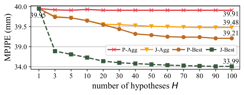
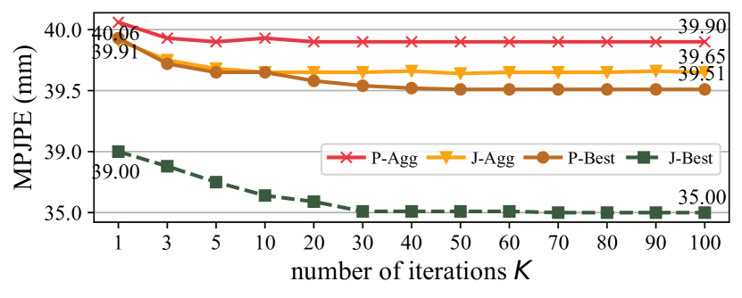
Figure 6: Ablation experiments on the number of hypotheses and iterations $H,K$. Top: $K$=10. Bottom: $H$=10.

Number of hypotheses and iterations.

Fig. 6 (Top) illustrates how performance fluctuates with the number of hypotheses under the four settings. They all start with the same performance ($H$=1) and then gradually diverge. 1) P-Best and J-Best: The error under J-Best is much lower than that under P-Best, which indicates that joint-level aggregation (J-Agg) has a higher upper-bound performance than pose-level aggregation (P-Agg). 2) P-Agg and J-Agg: Average and JPMA are used as the pose-level (P-Agg) and joint-level (J-Agg) methods, respectively. MPJPE under P-Agg stays around 39.9mm. It is because as $H$ increases, the mean of all hypotheses remains roughly the same, while the variance rises (Appendix D.3). This observation indicates that the average operation counteracts the advantage of increased diversity of hypotheses, leading to no improvement in performance. The error under J-Agg decreases as $H$ rises, which demonstrates that J-Agg makes better use of the diversity than P-Agg to achieve performance gains when $H$ increases. The performance of J-Agg is very close to the upper-bound performance of P-Agg (i.e., P-Best) when $H<20$. J-Agg is practical, but P-Best is not because the latter is agnostic in real-world applications, which highlights the advantages of J-Agg. Besides, there is still a performance gap between J-Agg (39.48mm) and J-Best (33.99mm), which shows that JPMA serves as a baseline method with considerable room for improvement.

Fig. 6 (Bottom) illustrates how performance fluctuates with the number of iterations. The general trend of the performance curves for the four settings is similar to that of the above experiment. Performance under P-Agg does not vary substantially with $K$. J-Agg and P-Best diverge after $K$=10. J-Best outperforms the other three settings by a wide margin. The performance of all settings saturates at $K$=30.

5 Conclusions

This paper presents D3DP with JPMA, a diffusion-based probabilistic method with joint-wise reprojection-based multi-hypothesis aggregation, for 3D human pose estimation. D3DP, which is compatible and customizable, generates multiple pose hypotheses. It progressively adds noise to clean 3D poses and reverses this process to reconstruct the original signals. To aggregate the generated pose hypotheses into a single 3D prediction, JPMA is proposed, which conducts joint-level aggregation based on reprojection errors. Compared with existing pose-level aggregation methods, JPMA exploits the merits of each joint and thus achieves exceptional performance. Experimental results on two benchmarks show that our method surpasses the state-of-the-art probabilistic and deterministic approaches.

Appendix A Preliminary: Diffusion Model

Following the notation of [42, 20, 8], we provide a detailed review of the diffusion models, which consist of a diffusion process and a reverse process.

Diffusion process. The diffusion process $q$ generates corrupted samples $\bm{y}_{1}$, $\bm{y}_{2}$, …, $\bm{y}_{T}$ by adding different levels of Gaussian noise to the original signal $\bm{y}_{0}$ at each timestep $t\in[0,T]$, which can be formulated as

$$\begin{split}q(\bm{y}_{1:T}|\bm{y}_{0})&\coloneqq\prod^{T}_{t=1}q(\bm{y}_{t}|\bm{y}_{t-1})\\ q(\bm{y}_{t}|\bm{y}_{t-1})&\coloneqq\mathcal{N}(\bm{y}_{t};\sqrt{1-\beta_{t}}\bm{y}_{t-1},\beta_{t}\bm{I})\end{split}$$ (7)

where $\beta_{t}$ is the noise variance schedule [42] and $\bm{I}$ denotes the identity matrix. Following Ho et al. [20], we can rewrite Eq. 7 in a form that requires no iteration to yield $\bm{y}_{t}$ from $\bm{y}_{0}$:

$$\begin{split}q(\bm{y}_{t}|\bm{y}_{0})&\coloneqq\mathcal{N}(\bm{y}_{t};\sqrt{\bar{\alpha}_{t}}\bm{y}_{0},(1-\bar{\alpha}_{t})\bm{I})\\ &\coloneqq\sqrt{\bar{\alpha}_{t}}\bm{y}_{0}+\epsilon\sqrt{1-\bar{\alpha}_{t}},\epsilon\sim\mathcal{N}(0,\bm{I})\end{split}$$ (8)

where $\bar{\alpha}_{t}\coloneqq\prod_{s=0}^{t}\alpha_{s}$ and $\alpha_{t}\coloneqq 1-\beta_{t}$. $\epsilon$ denotes the Gaussian noise. With a sufficiently large $T$ and reasonable noise schedule $\beta_{t}$, the distribution of $q(\bm{y}_{T})$ is nearly an isotropic Gaussian distribution $\mathcal{N}(0,\bm{I})$.

Reverse process. There are two ways to implement the reverse process $p$ using a neural network parameterized by $\theta$. One is by iterating $p_{\theta}(\bm{y}_{t-1}|\bm{y}_{t})$ multiple times until $\bm{y}_{0}$, and the other is by getting $\bm{y}_{0}$ in one step directly from $p_{\theta}(\bm{y}_{0}|\bm{y}_{t})$.

In the first case, it is found that the posterior $q(\bm{y}_{t-1}|\bm{y}_{t},\bm{y}_{0})$ can be formulated as a Gaussian distribution as well using the Bayes’ theorem:

$$\begin{split}q(\bm{y}_{t-1}|\bm{y}_{t},\bm{y}_{0})&=\mathcal{N}(\bm{y}_{t-1};\tilde{\mu}(\bm{y}_{t},\bm{y}_{0}),\tilde{\beta}_{t}\bm{I})\end{split}$$ (9)

where

$$\begin{split}\tilde{\beta}_{t}&\coloneqq\frac{1-\bar{\alpha}_{t-1}}{1-\bar{\alpha}_{t}}\beta_{t}\\ \tilde{\mu}_{t}(\bm{y}_{t},\bm{y}_{0})&\coloneqq\frac{\sqrt{\bar{\alpha}_{t-1}}\beta_{t}}{1-\bar{\alpha}_{t}}\bm{y}_{0}+\frac{\sqrt{\alpha_{t}}(1-\bar{\alpha}_{t-1})}{1-\bar{\alpha}_{t}}\bm{y}_{t}\end{split}$$ (10)

are the variance and mean of the Gaussian distribution, respectively. However, Eq. 9 depends on $\bm{y}_{0}$ to measure the posterior, which is unknown in advance. Instead, we approximate $q(\bm{y}_{t-1}|\bm{y}_{t},\bm{y}_{0})$ through

$$\begin{split}p_{\theta}(\bm{y}_{t-1}|\bm{y}_{t})&\coloneqq\mathcal{N}(\bm{y}_{t-1};\mu_{\theta}(\bm{y}_{t},t),\Sigma_{\theta}(\bm{y}_{t},t))\end{split}$$ (11)

where

$$\begin{split}\Sigma_{\theta}(\bm{y}_{t},t)&=\tilde{\beta}_{t}\bm{I}\\ \mu_{\theta}(\bm{y}_{t},t)&=\frac{1}{\sqrt{\alpha_{t}}}\left(\bm{y}_{t}-\frac{\beta_{t}}{\sqrt{1-\bar{\alpha}_{t}}}\epsilon_{\theta}(\bm{y}_{t},t)\right)\end{split}$$ (12)

where $\epsilon_{\theta}(\bm{y}_{t},t)$ is the noise predicted by the neural network, which is supervised by

$$\begin{split}\mathcal{L}=\mathbb{E}_{\bm{y}_{t},t,\epsilon}[||\epsilon_{\theta}(\bm{y}_{t},t)-\epsilon||^{2}]\end{split}$$ (13)

where $\epsilon\sim\mathcal{N}(0,\bm{I})$.

In the second case, we can directly predict the clean data from a learned network $f_{\theta}(\bm{y}_{t},t)$, which is supervised by

$$\begin{split}\mathcal{L}=\mathbb{E}_{\bm{y}_{t},t}[||f_{\theta}(\bm{y}_{t},t)-\bm{y}_{0}||^{2}]\end{split}$$ (14)

The difference between the above two cases lies in the prediction target of the network, which in the first case is the noise $\epsilon$ at each timestep, and in the second case is the original signal $\bm{y}_{0}$. We choose to predict $\bm{y}_{0}$ in this work.

Appendix B Preliminary: Projective Geometry

We refer to the process of a real-world object being photographed by a camera as the first projection. The obtained image is passed through the 3D pose estimator to predict multiple plausible 3D hypotheses. These hypotheses are projected a second time to the camera plane by JPMA, which is called reprojection. We introduce the reprojection function $\mathcal{P}(\cdot)$ in JPMA under two camera models: pinhole camera and distorted pinhole camera.

Pinhole camera.

We denote the 3D coordinate of a human joint in the camera coordinate system as $\left(X,Y,Z\right)$, and its reprojection to the camera plane as a 2D coordinate $\left(u,v\right)$. Then, the reprojection under a pinhole camera (with 4 intrinsic camera parameters) can be formulated by a perspective transformation:

$$\begin{split}X^{\prime}&=X/Z,\quad Y^{\prime}=Y/Z\\ u&=f_{x}\cdot X^{\prime}+c_{x}\\ v&=f_{y}\cdot Y^{\prime}+c_{y}\end{split}$$ (15)

where $f_{x},f_{y}$ are the focal lengths expressed in pixel units and $(c_{x},c_{y})$ is the principal point that is usually at the image center.

Distorted pinhole camera.

Real lenses will bring distortion to the ideal pinhole camera model, resulting in a distorted pinhole camera (with 9 intrinsic camera parameters). The distortion can be categorized into two types: 1) radial distortion, which is caused by flawed radial curvature of a lens and can be approximated by three parameters $k_{1},k_{2},k_{3}$; 2) tangential distortion, which arises mainly from the tilt of a lens with respect to the image sensor array and can be approximated by two parameters $p_{1},p_{2}$. When these two types of distortion are applied, Eq. 15 is extended as:

$$\begin{split}X^{\prime}&=X/Z,\quad Y^{\prime}=Y/Z\\ X_{\text{d}}&=X^{\prime}\cdot(d_{\text{r}}+d_{\text{t}})+p_{1}r^{2}\\ Y_{\text{d}}&=Y^{\prime}\cdot(d_{\text{r}}+d_{\text{t}})+p_{2}r^{2}\\ u&=f_{x}\cdot X_{\text{d}}+c_{x}\\ v&=f_{y}\cdot Y_{\text{d}}+c_{y}\end{split}$$ (16)

where $d_{\text{r}}=1+k_{1}r^{2}+k_{2}r^{4}+k_{3}r^{6},r=\sqrt{X^{\prime 2}+Y^{\prime 2}}$ and $d_{\text{t}}=2p_{1}X^{\prime 2}+2p_{2}Y^{\prime 2}$, following the formulation in [13].

For calibrated cameras, we use the ground truth intrinsic camera parameters for JPMA. Otherwise, we use a network to estimate the parameters, which is discussed in Section D.2.

Algorithm 1 D3DP Training

⬇

def training_loss(2dp, 3dp_gt, T):

# 2dp: [B, N, J, 2], 3dp_gt: [B, N, J, 3]

# T: maximum number of timesteps

# B: batch size, N: frame count, J: joint count

# Signal scaling

3dp_gt = 3dp_gt * scale

# Corrupt 3dp_gt

t = randint(0, T)             # timestep

noise = normal(mean=0, std=1) # noise: [B, N, J, 3]

alpha_cp = alpha_cumprod(t)

3dp_crpt = sqrt(    alpha_cp) * 3dp_gt +

  sqrt(1 - alpha_cp) * noise

# Denoise using a 3d pose estimator as backbone

3dp_pred = denoiser(3dp_crpt, 2dp, t)

# Set regression loss

loss = MSE(3dp_pred, 3dp_gt)

return loss

 alpha_cumprod(t): cumulative product of $\alpha_{i}$, i.e., $\prod_{i=1}^{t}\alpha_{i}$

Algorithm 2 D3DP Inference

⬇

def inference(2dp, T, K, H):

# 2dp: [B, N, J, 2], T: maximum number of timesteps

# K, H: number of iterations and hypotheses

# Initialize noisy 3d poses: [B, H, N, J, 3]

3dp_t = normal(mean=0, std=1)

# Sample timesteps uniformly

times = reversed(linespace(0, T, K + 1))

# [(T*(1-k/K), T*(1-(k+1)/K))], k = 0,...,K-1

time_pairs = list(zip(times[:-1], times[1:])

for t_now, t_next in zip(time_pairs):

# Predict 3dp_0 from 3dp_t

3dp_0 = denoiser(3dp_t, 2dp, t_now)

# Diffusion flipping

# Data augmentation using horizontal flipping

if augment:

2dp_hf = horiz_flipping(2dp)

3dp_t_hf = horiz_flipping(3dp_t)

3dp_0_hf = denoiser(3dp_t_hf, 2dp_hf, t_now)

3dp_0 = (3dp_0 + horiz_flipping(3dp_0_hf)) / 2

# Estimate 3dp_t at t_next

3dp_t = ddim_step(3dp_t, 3dp_0, t_now, t_next)

return 3dp_0

 linespace: generate evenly spaced values

Target	MPJPE$\downarrow$
noise	40.2
bestcolororiginal data	bestcolor40.0

(a) Regression target.

Location	MPJPE$\downarrow$
none	40.8
bestcolorfirst layer	bestcolor40.0
all layers	40.0

(b) Location of the added timestep embedding.

Type	MPJPE$\downarrow$
none	40.6
flipping-once	40.3
bestcolordiffusion-flipping	bestcolor40.0

(c) Data augmentation.

Type	Method	MPJPE$\downarrow$
bestcolorIF	bestcolorconcat	bestcolor40.0
EF	concat	40.9
EF	add	41.2
EF	CA	41.1

(d) 2D conditioning. IF: input fusion. EF: embedding fusion. CA: cross attention.

$T$	MPJPE$\downarrow$
100	40.8
500	40.2
bestcolor1000	bestcolor40.0
2000	40.3

(e) Maximum number of timesteps.

Table 5: Ablation experiments of D3DP on Human3.6M to justify the selection of each component. $H$=1, $K$=1. Default settings are shown in gray.

Appendix C Algorithm

Algorithm 1 provides the pseudo-code of D3DP training procedure. First, we scale the ground truth 3D pose $\bm{y}_{0}$ to control the signal-to-noise ratio. Then, a diffusion process is constructed from the scaled signal to the noisy 3D pose. Next, we train a denoiser to reverse this process by using the noisy 3D pose, 2D keypoints, and the timestep to predict the clean 3D pose $\widetilde{\bm{y}}_{0}$. The entire framework is supervised by an MSE loss: $\mathcal{L}=||\bm{y}_{0}-\widetilde{\bm{y}}_{0}||_{2}$. By using this simple optimization objective, we avoid issues of sensitivity to hyperparameters (e.g., balance factor between different loss functions) and training instability encountered in previous methods [63, 34].

Algorithm 2 provides the pseudo-code of D3DP inference procedure. We start by sampling $H$ initial 3D poses from a Gaussian distribution and use the number of iterations $K$ to determine the timestep for each iteration. In each iteration, noisy 3D poses are sent into the denoiser to estimate the uncontaminated 3D poses, which are used by DDIM to derive noisy inputs for the denoiser in the next iteration.

In addition, we combine D3DP with a common data augmentation scheme (i.e., horizontal flipping) in deterministic 3D pose estimation [70, 51, 68, 46], and propose diffusion-flipping. Specifically, we horizontally flip input 2D keypoints as well as noisy 3D poses. The denoiser is then employed to produce the flipped predictions, which are flipped back and averaged with the original predictions to obtain the final 3D poses. The above steps are repeated in each iteration. Compared with previous approaches, the proposed method extends the data augmentation from once to $K$ times, which reduces the cumulative error and increases the accuracy of predictions.

Iteration	1	2	3	4	5
noise $\epsilon_{t}$	48.6	43.5	41.0	40.5	40.0
original data $\bm{y}_{0}$	39.9	39.9	39.8	39.8	39.7

Table 6: Performance of two regression targets after each iteration. MPJPE$\downarrow$ is reported. H=K=5. J-Agg is used.

Appendix D Additional Ablation Study

D.1 Components of D3DP

We conduct more ablation experiments on Human3.6M to study the design of D3DP in detail.

Regression target.

We implement two alternatives: predicting the noise $\epsilon_{t}$ at each timestep of the reverse process or predicting the original 3D data $\bm{y}_{0}$. As shown in Table 5a, the latter achieves better results.

Note that the difference between our work and other concurrent diffusion-based methods [22, 18, 14] mainly lies in the regression target. The regression target of our model is the original 3D data $\bm{y}_{0}$, while theirs is the noise $\epsilon_{t}$ at each timestep. Table 5a shows our method outperforms theirs. Further experiments (Table 6) reveal that predicting $\bm{y}_{0}$ yields good performance even in early iterations, while predicting $\epsilon_{t}$ does not. This is because in early iterations, when the input $\bm{y}_{t}$ is extremely noisy, it is more effective to predict the original signal $\bm{y}_{0}$ directly than to obtain $\bm{y}_{0}$ by predicting the noise $\epsilon_{t}$ and then subtracting it from $\bm{y}_{t}$. This property is valuable for real-time processing. For example, when $K$ is fixed and computational resources are inadequate, the algorithm is required to produce predictions after the first iteration. Our method of predicting $\bm{y}_{0}$ still achieves satisfactory results, while theirs of predicting $\epsilon_{t}$ does not.

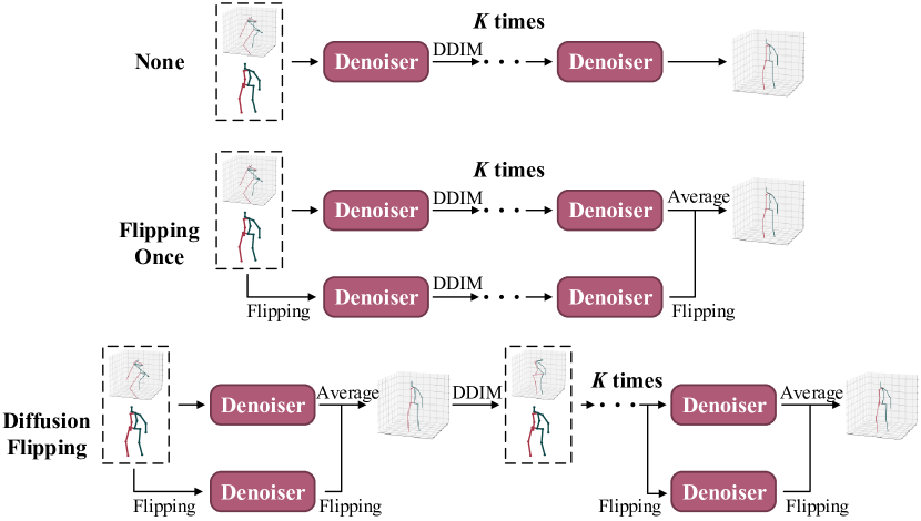
Figure 7: Detailed architectures of three data augmentation approaches.

Location of the timestep embedding.

We add the timestep embedding to the network in a similar way as the positional embedding [58]. Table 5b shows that adding it to the first layer of the network performs the same as all layers, hence the former is chosen for simplicity. Experimental results demonstrate that timestep embedding is crucial to the denoising process.

Data augmentation.

Three data augmentation approaches are compared in Table 5c, including 1) no augmentation; 2) flipping-once, which flips the input, conducts denoising for $K$ times, and flips the prediction again. The flipped prediction is then averaged with the unflipped prediction in the original branch to yield the final output; 3) diffusion-flipping, which applies the flip-denoise-flip process to each timestep ($K$ times). The detailed architectures of these three approaches are shown in Fig. 7. Our diffusion-flipping achieves the best results because it averages the 3D poses of the original and flipped branches at each timestep, preventing the accumulation of errors. Other concurrent diffusion-based methods [22, 18, 14] don’t use any augmentation or use the flipping-once method. Therefore, our model is more effective than theirs.

2D conditioning.

As shown in Table 5d, we evaluate multiple fusion methods (concatenation, addition, and cross attention [58]) in two fusion types (input fusion and embedding fusion). For embedding fusion, two additional spatio-temporal Transformer layers are used to extract 2D features, after which these features are fused into the denoiser. The best fusion approach is concatenating noisy 3D poses and 2D conditions on the input side, which provides a fast and effective way to modify existing 3D pose estimators to fit the diffusion framework.

Maximum number of timesteps.

Table 5e indicates that the best performance can be achieved by setting an appropriate maximum number of timesteps. When $T$ is too small, we cannot diffuse the ground truth 3D poses to a Gaussian distribution during training, so the denoiser has trouble recovering a clean pose from Gaussian noise during inference. When $T$ is too large, excessive samples become pure noise after diffusion. Then, the training process of the denoiser is affected and the denoiser cannot generalize well to 3D poses with varying levels of noise (i.e., 3D poses at different timesteps) during inference.

Compatibility.

The denoiser has the compatibility to use existing 3D human pose estimators as the backbone. We run our pipeline on a few other 3D estimators [51, 70, 35, 46]. Table 7 shows that our approach achieves performance gains over different backbone networks, which verifies the compatibility and versatility.

Backbone	P-STMO [51]	PoseFormer [70]	STE [35]	TCN [46]
w/o diffusion	43.7	47.6	44.6	46.4
w/ diffusion	42.2	45.7	43.8	44.5

Table 7: Performance using other 3D estimators as backbone. MPJPE$\downarrow$ is reported. H=K=1.

Camera Model	Access	MPJPE$\downarrow$
w/ distortion	GT	39.74
w/o distortion	GT	39.80
w/ distortion	estimated	39.78
w/o distortion	estimated	39.82

Table 8: Impact of different camera models and different ways of accessing intrinsic camera parameters. $H$=5, $K$=5. GT: ground truth. J-Agg setting is used.

D.2 Intrinsic Camera Parameters in JPMA

As shown in Table 8, we investigate the effect of two factors on the performance of JPMA: 1) the camera model, including pinhole camera (w/o distortion) or distorted pinhole camera (w/ distortion); 2) the way of accessing the intrinsic camera parameters, including using the ground truth (GT) or using a 2-layer MLPs to estimate the parameters (estimated). When the ground truth intrinsic camera parameters are used, the ideal pinhole camera model without distortion shows a performance degradation of 0.06mm compared with the case with distortion. When a neural network is utilized to estimate the parameters (the ground truth is not available), the performance drops by only 0.04mm and 0.02mm in distorted and distortion-free cases, respectively. These results indicate that the proposed JPMA method is robust to the noise caused by incorrect camera models or inaccurate estimations of intrinsic camera parameters.

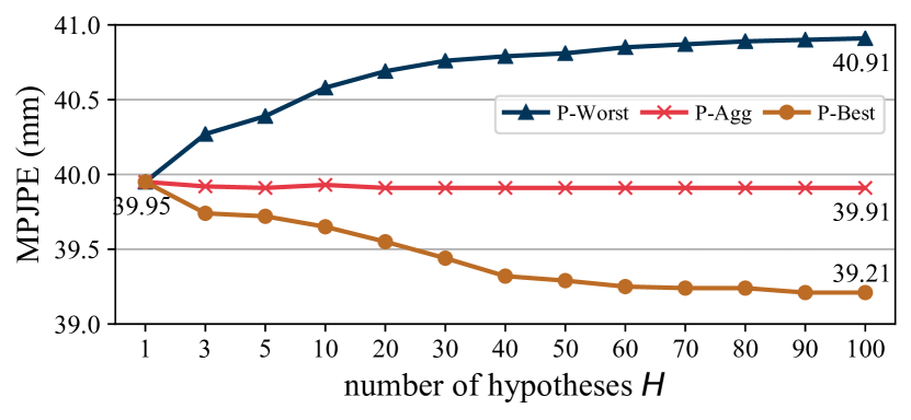
Figure 8: Effect of different numbers of hypotheses $H$ on the performance of the best, worst, and average hypotheses. $K$=10.

D.3 Variance of Hypotheses

Fig. 8 shows how the performance of the best, worst, and average hypotheses changes with the number of hypotheses $H$. As $H$ increases, the performance of the average hypothesis remains essentially unchanged, with the worst hypothesis getting worse and the best hypothesis getting better. This result validates the statement in the main paper that the mean of all hypotheses remains roughly the same (the error stays around 39.9mm), while the variance rises.

Appendix E Additional Quantitative Results

Table 9 provides quantitative comparisons between our D3DP with JPMA and the state-of-the-art approaches on Human3.6M when P-MPJPE is reported using 2D keypoints obtained from 2D detectors as inputs. Table 10 shows the results when MPJPE is reported using ground truth 2D keypoints as inputs. Without bells and whistles, D3DP transforms an existing deterministic 3D pose estimator into a probabilistic version with simple modifications and achieves considerable performance gains. Our method produces favorable results under conventional pose-level settings (P-Agg and P-Best), and the performance is further enhanced under the proposed joint-level settings (J-Agg and J-Best), which demonstrates the effectiveness of disentangling the hypothesis at the joint level. Experimental results show that the proposed method surpasses the others by a wide margin.

Deterministic Methods
P-MPJPE		Dir.	Disc.	Eat	Greet	Phone	Photo	Pose	Pur.	Sit	SitD.	Smoke	Wait	WalkD.	Walk	WalkT.	Avg
TCN [46] ($N$=243)*	CVPR’19	34.1	36.1	34.4	37.2	36.4	42.2	34.4	33.6	45.0	52.5	37.4	33.8	37.8	25.6	27.3	36.5
RIE [52] ($N$=243)*	MM’21	32.5	36.2	33.2	35.3	35.6	42.1	32.6	31.9	42.6	47.9	36.6	32.1	34.8	24.2	25.8	35.0
Anatomy [9] ($N$=243)*	TCSVT’21	32.6	35.1	32.8	35.4	36.3	40.4	32.4	32.3	42.7	49.0	36.8	32.4	36.0	24.9	26.5	35.0
PoseFormer [70] ($N$=81)*	ICCV’21	32.5	34.8	32.6	34.6	35.3	39.5	32.1	32.0	42.8	48.5	34.8	32.4	35.3	24.5	36.0	34.6
U-CDGCN [23] ($N$=96)*	MM’21	29.8	34.4	31.9	31.5	35.1	40.0	30.3	30.8	42.6	49.0	35.9	31.8	35.0	25.7	23.6	33.8
STE [35] ($N$=351)*	TMM’22	32.7	35.5	32.5	35.4	35.9	41.6	33.0	31.9	45.1	50.1	36.3	33.5	35.1	23.9	25.0	35.2
P-STMO [51] ($N$=243)*	ECCV’22	31.3	35.2	32.9	33.9	35.4	39.3	32.5	31.5	44.6	48.2	36.3	32.9	34.4	23.8	23.9	34.4
MixSTE [68] ($N$=243)*	CVPR’22	30.8	33.1	30.3	31.8	33.1	39.1	31.1	30.5	42.5	44.5	34.0	30.8	32.7	22.1	22.9	32.6
MixSTE [68] ($N$=243)*$\ddagger$	CVPR’22	30.8	32.7	30.6	31.9	33.1	38.6	30.8	30.4	42.4	46.4	34.2	30.7	32.3	21.8	22.6	32.6
DUE [67] ($N$=300)*	MM’22	30.3	34.6	29.6	31.7	31.6	38.9	31.8	31.9	39.2	42.8	32.1	32.6	31.4	25.1	23.8	32.5
bestcolorD3DP ($N$=243, $H$=1, $K$=1)*	bestcolor	bestcolor30.6	bestcolor32.5	bestcolor29.1	bestcolor31.0	bestcolor31.9	bestcolor37.6	bestcolor30.3	bestcolor29.4	bestcolor40.6	bestcolor43.6	bestcolor33.3	bestcolor30.5	bestcolor31.4	bestcolor21.5	bestcolor22.4	bestcolor31.7
Probabilistic Methods
P-MPJPE		Dir.	Disc.	Eat	Greet	Phone	Photo	Pose	Pur.	Sit	SitD.	Smoke	Wait	WalkD.	Walk	WalkT.	Avg
CVAE [53] ($N$=1, $H$=200, P-Agg)	ICCV’19	35.3	35.9	45.8	42.0	40.9	52.6	36.9	35.8	43.5	51.9	44.3	38.8	45.5	29.4	34.3	40.9
GAN [34] ($N$=1, $H$=10, P-Agg)	BMVC’20	42.1	44.7	45.4	51.0	49.3	51.5	41.2	46.2	57.5	70.8	48.7	44.1	50.8	42.1	43.7	48.7
GraphMDN [44] ($N$=1, $H$=5, P-Agg)	IJCNN’21	39.7	43.4	44.0	46.2	48.8	54.5	39.4	41.1	55.0	69.0	48.0	43.7	49.6	38.4	42.4	46.9
NF [63] ($N$=1, $H$=1, P-Agg)	ICCV’21	37.8	41.7	42.1	41.8	46.5	50.2	38.0	39.2	51.7	61.8	45.4	42.6	45.7	33.7	38.5	43.8
MHFormer [36] ($N$=351, $H$=3, P-Agg)*	CVPR’22	31.5	34.9	32.8	33.6	35.3	39.6	32.0	32.2	43.5	48.7	36.4	32.6	34.3	23.9	25.1	34.4
bestcolorD3DP ($N$=243, $H$=1, $K$=1, P-Agg)*	bestcolor	bestcolor30.6	bestcolor32.5	bestcolor29.1	bestcolor31.0	bestcolor31.9	bestcolor37.6	bestcolor30.3	bestcolor29.4	bestcolor40.6	bestcolor43.6	bestcolor33.3	bestcolor30.5	bestcolor31.4	bestcolor21.5	bestcolor22.4	bestcolor31.7
bestcolorD3DP ($N$=243, $H$=20, $K$=10, P-Agg)*	bestcolor	bestcolor30.6	bestcolor32.5	bestcolor29.1	bestcolor30.9	bestcolor31.9	bestcolor37.5	bestcolor30.2	bestcolor29.4	bestcolor40.6	bestcolor43.4	bestcolor33.3	bestcolor30.4	bestcolor31.4	bestcolor21.5	bestcolor22.4	bestcolor31.7
bestcolorD3DP ($N$=243, $H$=20, $K$=10, J-Agg)*	bestcolor	bestcolor30.6	bestcolor32.4	bestcolor29.2	bestcolor30.9	bestcolor31.9	bestcolor37.4	bestcolor30.2	bestcolor29.3	bestcolor40.4	bestcolor43.2	bestcolor33.2	bestcolor30.4	bestcolor31.3	bestcolor21.5	bestcolor22.3	bestcolor31.6
MDN [33] ($N$=1, $H$=5, P-Best$\sharp$)	CVPR’19	35.5	39.8	41.3	42.3	46.0	48.9	36.9	37.3	51.0	60.6	44.9	40.2	44.1	33.1	36.9	42.6
CVAE [53] ($N$=1, $H$=200, P-Best$\sharp$)	ICCV’19	27.6	27.5	34.9	32.3	33.3	42.7	28.7	28.0	36.1	42.7	36.0	30.7	37.6	24.3	27.1	32.7
GAN [34] ($N$=1, $H$=10, P-Best$\sharp$)	BMVC’20	38.5	41.7	39.6	45.2	45.8	46.5	37.8	42.7	52.4	62.9	45.3	40.9	45.3	38.6	38.4	44.3
GraphMDN [44] ($N$=1, $H$=200, P-Best$\sharp$)	IJCNN’21	30.8	34.7	33.6	34.2	39.6	42.2	31.0	31.9	42.9	53.5	38.1	34.1	38.0	29.6	31.1	36.3
NF [63] ($N$=1, $H$=200, P-Best$\sharp$)	ICCV’21	27.9	31.4	29.7	30.2	34.9	37.1	27.3	28.2	39.0	46.1	34.2	32.3	33.6	26.1	27.5	32.4
bestcolorD3DP ($N$=243, $H$=1, $K$=1, P-Best$\sharp$)*	bestcolor	bestcolor30.6	bestcolor32.5	bestcolor29.1	bestcolor31.0	bestcolor31.9	bestcolor37.6	bestcolor30.3	bestcolor29.4	bestcolor40.6	bestcolor43.6	bestcolor33.3	bestcolor30.5	bestcolor31.4	bestcolor21.5	bestcolor22.4	bestcolor31.7
bestcolorD3DP ($N$=243, $H$=20, $K$=10, P-Best$\sharp$)*	bestcolor	bestcolor30.2	bestcolor32.1	bestcolor28.8	bestcolor30.4	bestcolor31.5	bestcolor37.0	bestcolor29.8	bestcolor28.9	bestcolor39.9	bestcolor42.4	bestcolor32.8	bestcolor30.0	bestcolor30.9	bestcolor21.3	bestcolor22.1	bestcolor31.2
bestcolorD3DP ($N$=243, $H$=20, $K$=10, J-Best$\sharp$)*	bestcolor	bestcolor27.5	bestcolor29.4	bestcolor26.6	bestcolor27.7	bestcolor29.2	bestcolor34.3	bestcolor27.5	bestcolor26.2	bestcolor37.3	bestcolor39.0	bestcolor30.3	bestcolor27.7	bestcolor28.2	bestcolor19.6	bestcolor20.3	bestcolor28.7

Table 9: Results on Human3.6M in millimeters under P-MPJPE. $N,H,K$: the number of input frames, hypotheses, and iterations of the proposed D3DP. ($\ddagger$) - Our implementation. ($\sharp$) - Not feasible in real-world applications. (*) - Use CPN  [11] as the 2D keypoint detector to generate the inputs. Red: Best. Blue: Second best. Gray: our method.

Deterministic Methods
MPJPE		Dir.	Disc.	Eat	Greet	Phone	Photo	Pose	Pur.	Sit	SitD.	Smoke	Wait	WalkD.	Walk	WalkT.	Avg
TCN [46] ($N$=243)	CVPR’19	35.2	40.2	32.7	35.7	38.2	45.5	40.6	36.1	48.8	47.3	37.8	39.7	38.7	27.8	29.5	37.8
SRNet [65] ($N$=243)	ECCV’20	34.8	32.1	28.5	30.7	31.4	36.9	35.6	30.5	38.9	40.5	32.5	31.0	29.9	22.5	24.5	32.0
Anatomy [9] ($N$=243)	TCSVT’21	-	-	-	-	-	-	-	-	-	-	-	-	-	-	-	32.3
PoseFormer [70] ($N$=81)	ICCV’21	30.0	33.6	29.9	31.0	30.2	33.3	34.8	31.4	37.8	38.6	31.7	31.5	29.0	23.3	23.1	31.3
RIE [52] ($N$=243)	MM’21	29.5	30.8	28.8	29.1	30.7	35.2	31.7	27.8	34.5	36.0	30.3	29.4	28.9	24.1	24.7	30.1
Ray3D [66] ($N$=9)	CVPR’22	31.2	35.7	34.6	33.6	35.0	37.5	37.2	30.9	42.5	41.3	34.6	36.5	32.0	29.7	28.9	34.4
P-STMO [51] ($N$=243)	ECCV’22	28.5	30.1	28.6	27.9	29.8	33.2	31.3	27.8	36.0	37.4	29.7	29.5	28.1	21.0	21.0	29.3
STE [35] ($N$=351)	TMM’22	27.1	29.4	26.5	27.1	28.6	33.0	30.7	26.8	38.2	34.7	29.1	29.8	26.8	19.1	19.8	28.5
DUE [67] ($N$=300)	MM’22	22.1	23.1	20.1	22.7	21.3	24.1	23.6	21.6	26.3	24.8	21.7	21.4	21.8	16.7	18.7	22.0
MixSTE [68] ($N$=243)	CVPR’22	21.6	22.0	20.4	21.0	20.8	26.3	24.7	21.9	26.9	24.9	21.2	21.5	20.8	14.7	15.7	21.6
MixSTE [68] ($N$=243)$\ddagger$	CVPR’22	22.9	21.7	21.0	21.4	20.8	23.5	24.1	21.8	25.3	23.5	21.4	20.1	19.5	15.3	16.6	21.3
bestcolorD3DP ($N$=243, $H$=1, $K$=1)	bestcolor	bestcolor19.9	bestcolor19.6	bestcolor19.7	bestcolor19.3	bestcolor20.2	bestcolor22.7	bestcolor21.5	bestcolor19.2	bestcolor25.5	bestcolor24.0	bestcolor20.1	bestcolor18.9	bestcolor19.0	bestcolor14.0	bestcolor14.5	bestcolor19.9
Probabilistic Methods
MPJPE		Dir.	Disc.	Eat	Greet	Phone	Photo	Pose	Pur.	Sit	SitD.	Smoke	Wait	WalkD.	Walk	WalkT.	Avg
GraphMDN [44] ($N$=1, $H$=5, P-Agg)	IJCNN’21	33.9	39.9	33.0	35.4	36.8	44.4	38.9	33.0	41.0	50.0	36.4	38.3	37.8	28.2	31.5	37.2
MHFormer [36]($N$=351, $H$=3, P-Agg)	CVPR’22	27.7	32.1	29.1	28.9	30.0	33.9	33.0	31.2	37.0	39.3	30.3	31.0	29.4	22.2	23.0	30.5
bestcolorD3DP ($N$=243, $H$=1, $K$=1, P-Agg)	bestcolor	bestcolor19.9	bestcolor19.6	bestcolor19.7	bestcolor19.3	bestcolor20.2	bestcolor22.7	bestcolor21.5	bestcolor19.2	bestcolor25.5	bestcolor24.0	bestcolor20.1	bestcolor18.9	bestcolor19.0	bestcolor14.0	bestcolor14.5	bestcolor19.9
bestcolorD3DP ($N$=243, $H$=20, $K$=10, P-Agg)	bestcolor	bestcolor19.9	bestcolor19.5	bestcolor19.6	bestcolor19.2	bestcolor20.1	bestcolor22.4	bestcolor21.5	bestcolor19.1	bestcolor25.4	bestcolor23.7	bestcolor20.0	bestcolor18.9	bestcolor18.8	bestcolor14.0	bestcolor14.5	bestcolor19.8
bestcolorD3DP ($N$=243, $H$=20, $K$=10, J-Agg)	bestcolor	bestcolor19.9	bestcolor19.4	bestcolor19.4	bestcolor19.0	bestcolor19.8	bestcolor22.0	bestcolor21.4	bestcolor19.1	bestcolor24.8	bestcolor23.2	bestcolor19.6	bestcolor18.7	bestcolor18.6	bestcolor14.0	bestcolor14.5	bestcolor19.6
GAN [34] ($N$=1, $H$=10, P-Best$\sharp$)	BMVC’20	54.8	61.9	48.6	63.6	55.8	73.7	59.0	61.3	62.2	85.7	52.8	60.2	57.5	51.3	56.8	60.0
GraphMDN [44] ($N$=1, $H$=5, P-Best$\sharp$)	IJCNN’21	28.9	34.5	28.2	30.2	31.5	38.5	32.3	28.6	35.7	43.3	31.9	32.1	33.3	25.2	27.8	31.8
bestcolorD3DP ($N$=243, $H$=1, $K$=1, P-Best$\sharp$)	bestcolor	bestcolor19.9	bestcolor19.6	bestcolor19.7	bestcolor19.3	bestcolor20.2	bestcolor22.7	bestcolor21.5	bestcolor19.2	bestcolor25.5	bestcolor24.0	bestcolor20.1	bestcolor18.9	bestcolor19.0	bestcolor14.0	bestcolor14.5	bestcolor19.9
bestcolorD3DP ($N$=243, $H$=20, $K$=10, P-Best$\sharp$)	bestcolor	bestcolor19.7	bestcolor19.3	bestcolor19.2	bestcolor18.8	bestcolor19.6	bestcolor21.9	bestcolor21.2	bestcolor18.6	bestcolor24.7	bestcolor23.0	bestcolor19.4	bestcolor18.4	bestcolor18.4	bestcolor13.9	bestcolor14.4	bestcolor19.4
bestcolorD3DP ($N$=243, $H$=20, $K$=10, J-Best$\sharp$)	bestcolor	bestcolor18.7	bestcolor18.2	bestcolor18.4	bestcolor17.8	bestcolor18.6	bestcolor20.9	bestcolor20.2	bestcolor17.7	bestcolor23.8	bestcolor21.8	bestcolor18.5	bestcolor17.4	bestcolor17.4	bestcolor13.1	bestcolor13.6	bestcolor18.4

Table 10: Results on Human3.6M in millimeters under MPJPE. $N,H,K$: the number of input frames, hypotheses, and iterations of the proposed D3DP. ($\ddagger$) - Our implementation. ($\sharp$) - Not feasible in real-world applications. The ground truth 2D keypoints are used as inputs. Red: Best. Blue: Second best. Gray: our method.

Appendix F Additional Qualitative Results

F.1 Different Numbers of Hypotheses and
Iterations

We show the qualitative results under different numbers of hypotheses $H$ and iterations $K$ in Fig. 9. When $H$ increases (first row), the mean of hypotheses is basically unchanged while the variance increases, which is consistent with the conclusion in Section D.3. When $K$ increases (second row), the variance also raises gradually, meaning that the diversity of hypotheses is improved. This is because DDIM re-adds different noise to the predicted 3D poses to generate inputs for the next iteration, resulting in a progressive increase in the gap between different hypotheses as $K$ grows. When the variance is small, the 2D reprojections of all hypotheses are close to each other, which may affect the performance of JPMA (middle left: the solid red line is not better than the green one in the left foot region). When $H,K$ are fixed (third row), we show the results of the 3D hypotheses estimated in each iteration. As $k$ increases, the diversity of hypotheses is improved and the advantage of JPMA over average becomes apparent.

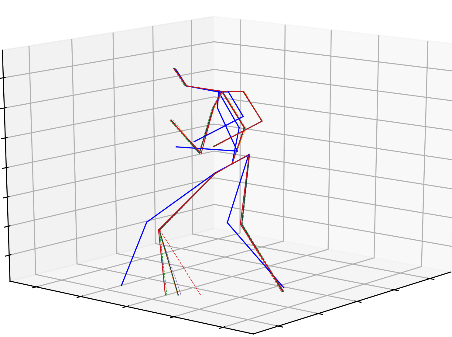
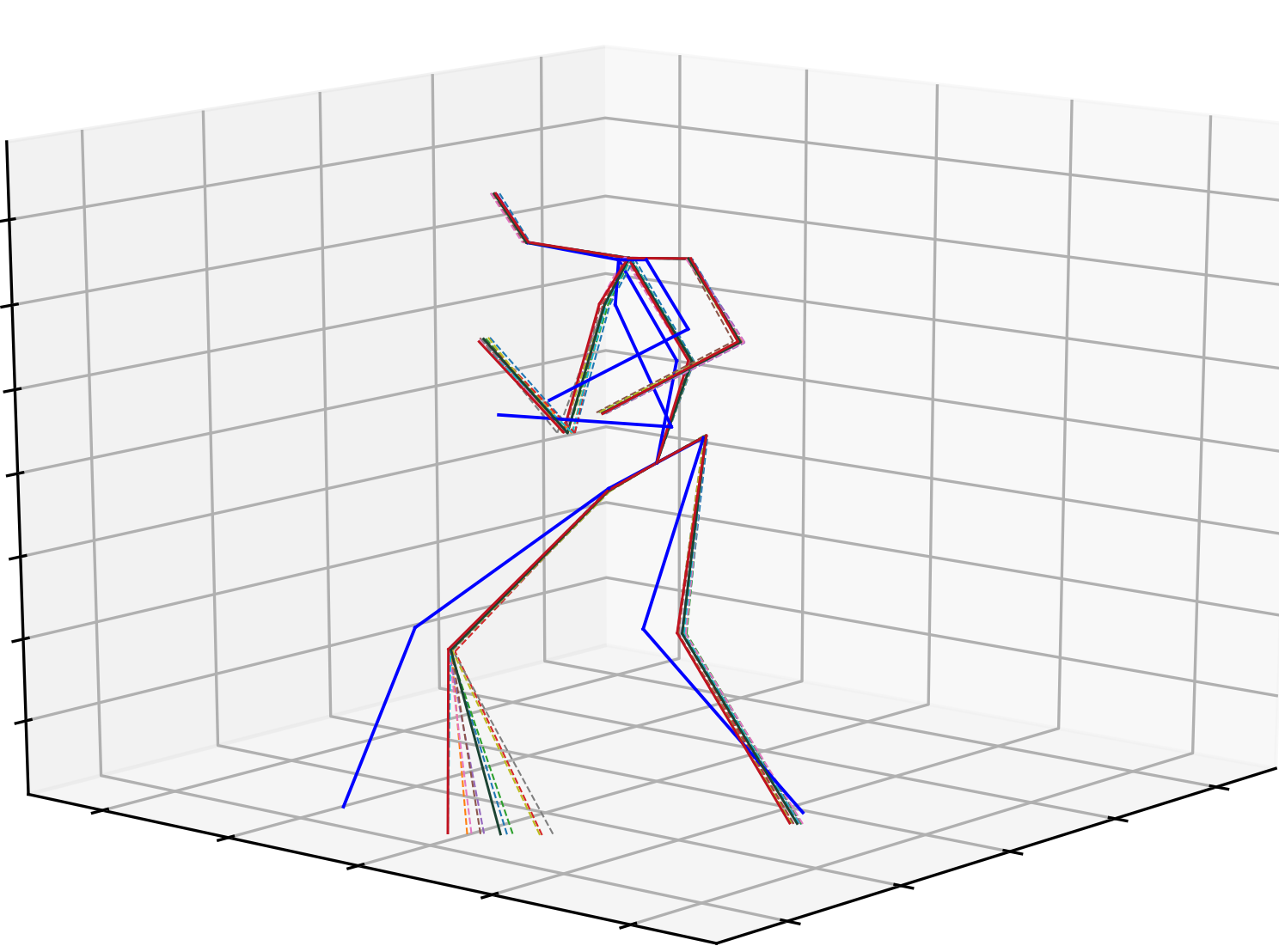
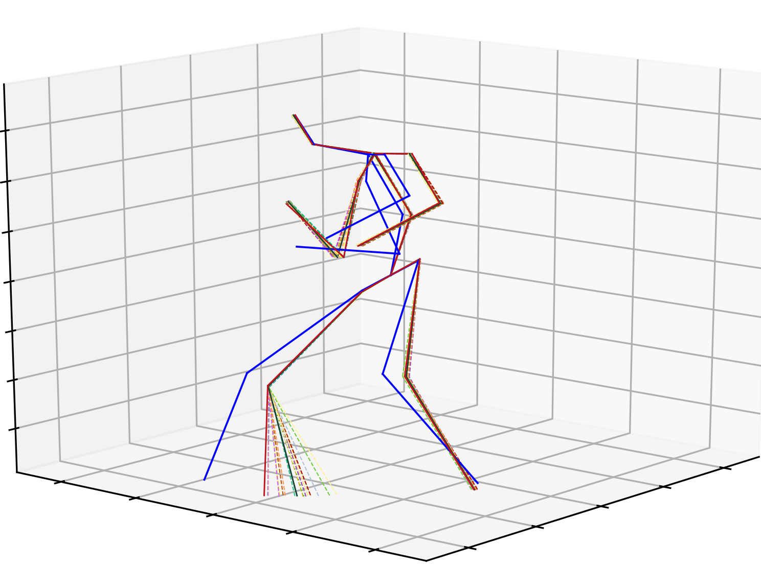
$H$=5,$K$=5,$k$=4	$H$=10,$K$=5,$k$=4	$H$=20,$K$=5,$k$=4
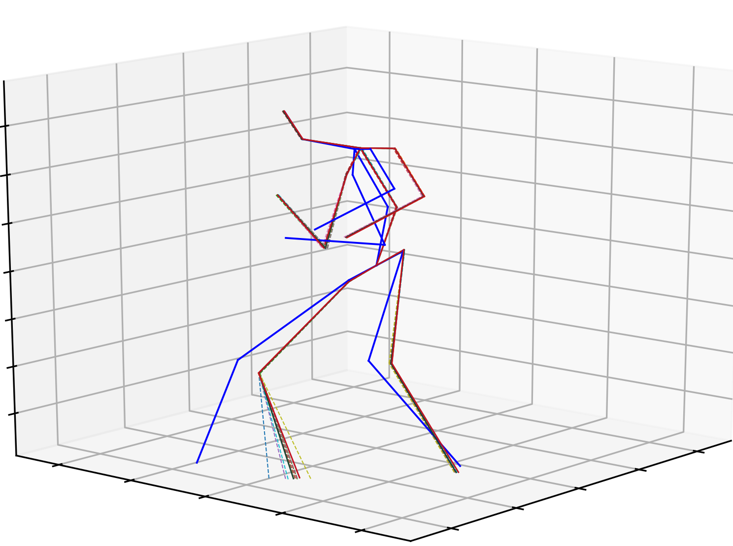
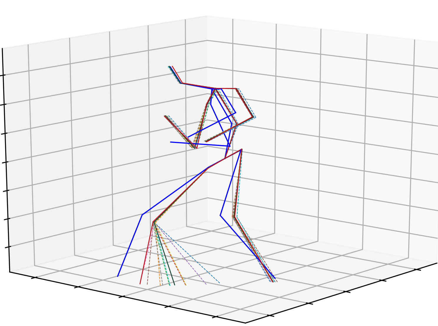
$H$=10,$K$=2,$k$=1	$H$=10,$K$=5,$k$=4	$H$=10,$K$=10,$k$=9
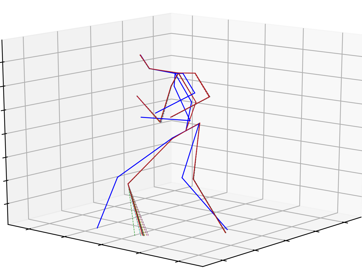
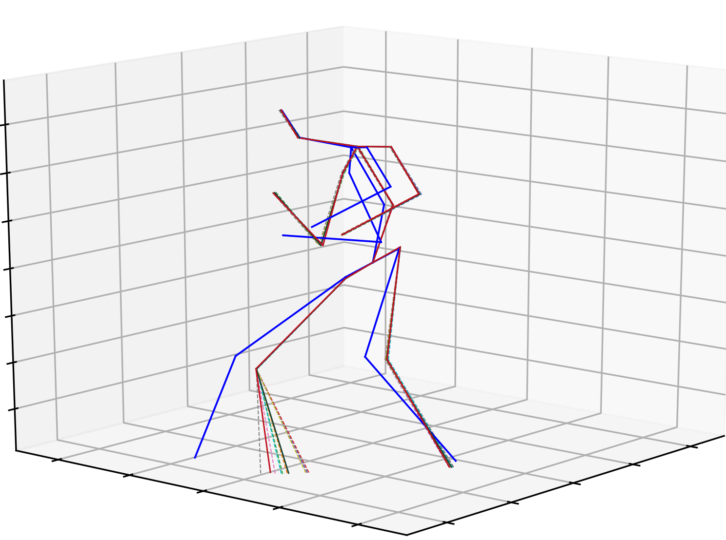
$H$=10,$K$=10,$k$=0	$H$=10,$K$=10,$k$=5	$H$=10,$K$=10,$k$=9

Figure 9: Qualitative results under different numbers of hypotheses $H$ and iterations $K$. Top: $H$ varies, when $K$=5. The results are the outputs of the last iteration, i.e., $k$=4 for all three subfigures. Middle: $K$ varies, when $H$=10. The results are the outputs of the last iteration, i.e., $k$=1, 4, 9 for three subfigures respectively. Bottom: $H$=10, $K$=10. The results are the outputs of the first, intermediate, and last iterations, i.e., $k$=0, 5, 9 for three subfigures respectively. Dashed line: predicted 3D pose hypotheses. Each color represents an individual hypothesis. Solid blue line: ground truth 3D poses. Solid red line: the final prediction obtained by using JPMA as the aggregation method. Solid green line: the final prediction obtained by using average as the aggregation method.

F.2 In-the-Wild Videos

We train our method on Human3.6M dataset and evaluate on in-the-wild videos from 3DPW [60], Penn Action [69], JHMDB [27], and youtube. We use AlphaPose [17] as the 2D keypoint detector to generate 2D poses. As shown in Fig. 10, our method achieves satisfactory performance in most of the frames. For the cases of severe occlusion ($\text{3}^{\text{rd}}$ row), fast motion ($\text{5}^{\text{th}}$ row), low illumination ($\text{7}^{\text{th}}$ row), and rare poses ($\text{8}^{\text{th}}$ row), the proposed method generates highly uncertain predictions to represent the possible locations of 3D poses. Besides, our method can also generalize to animations ($\text{8}^{\text{th}}$ row) and monkey poses ($\text{9}^{\text{th}}$ row) because 2D keypoints are used as inputs, excluding the interference of complex textures. Theoretically, our method can be applied to any type of humanoid 3D pose estimation.

F.3 Analysis of Failure Cases

Our method may fail under the previously mentioned cases such as severe occlusions, fast motion, rare poses, etc. The $\text{3}^{\text{rd}}$ row of Fig. 10 shows a person walking through the woods. Most of her body is occluded and our approach cannot obtain a very accurate result in this case. Besides, the person in the $\text{6}^{\text{th}}$ row of Fig. 10 raises his hand above his head, a movement that is rare in the training set. Our method fails to generalize to this pose and therefore produces incorrect predictions.

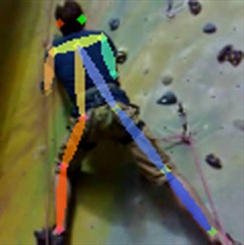
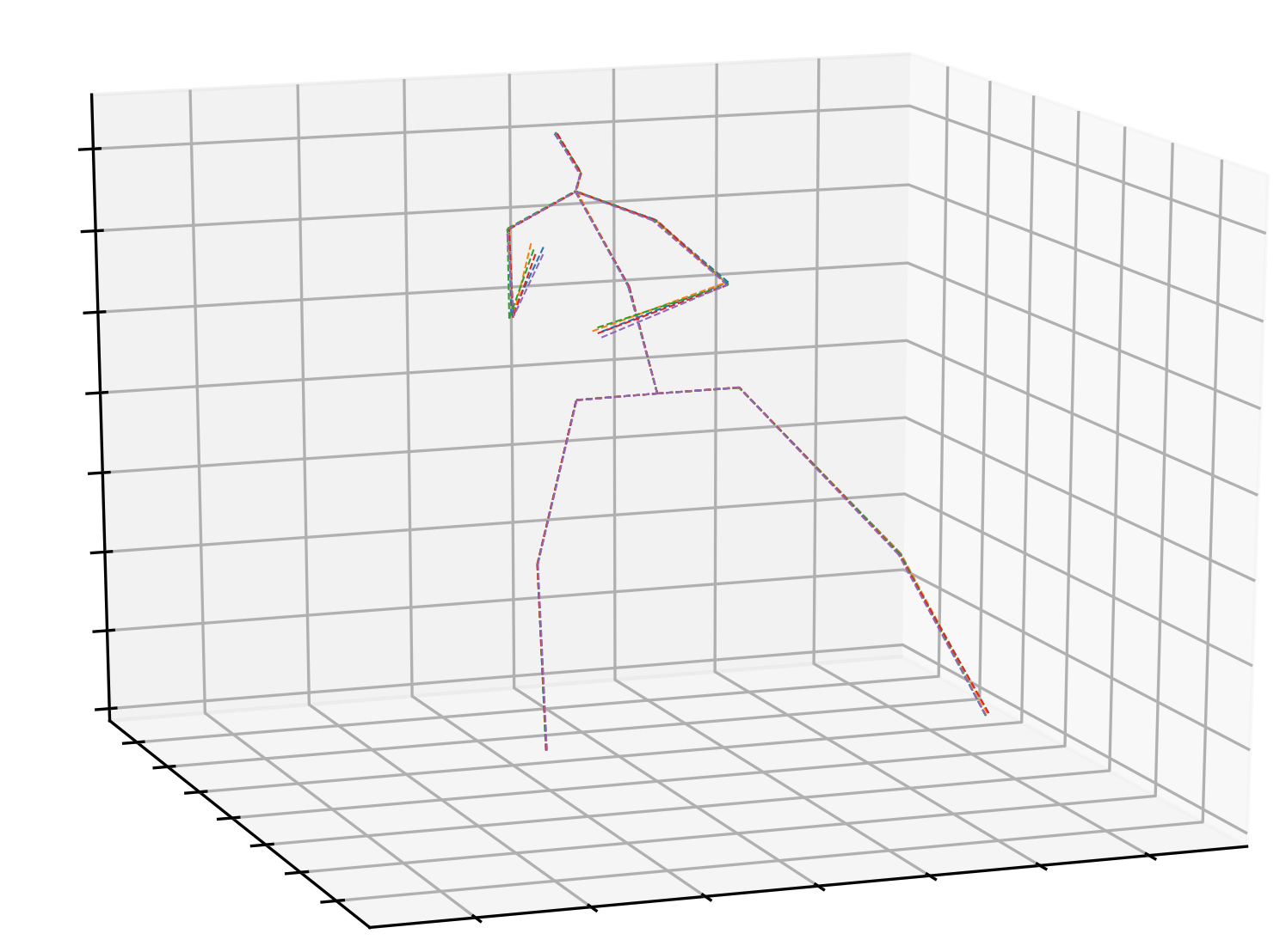
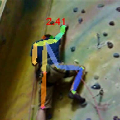
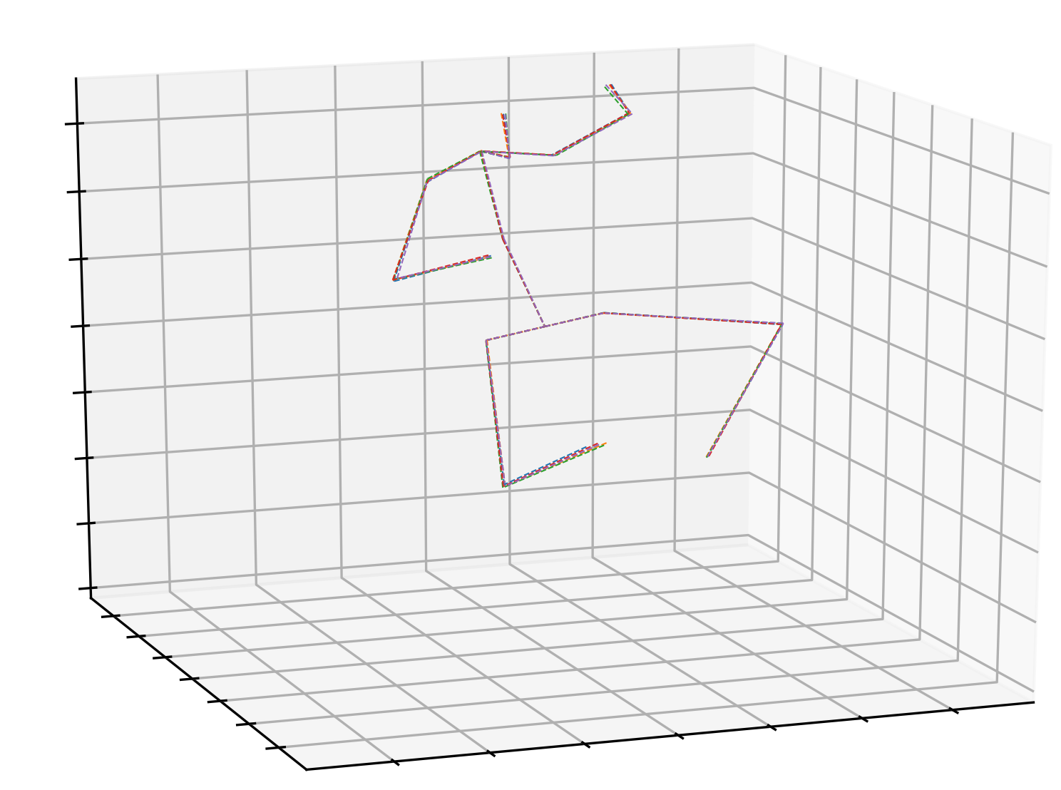
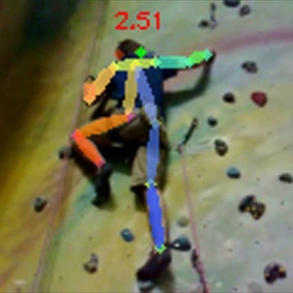
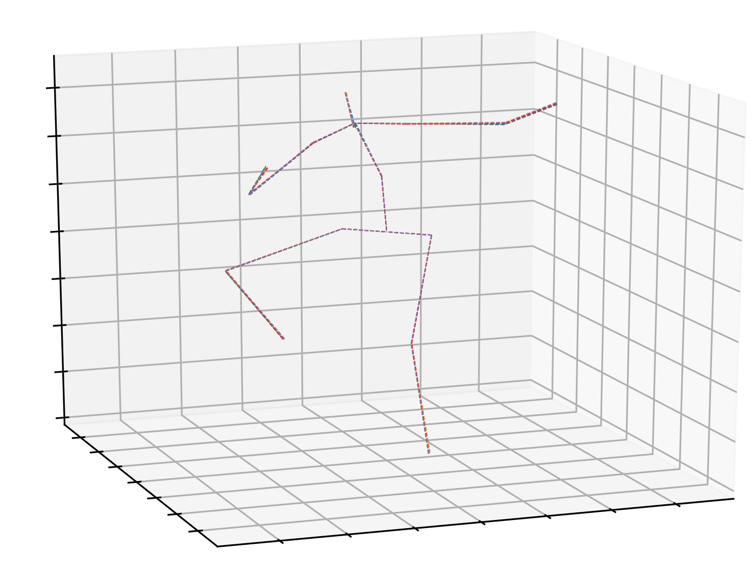
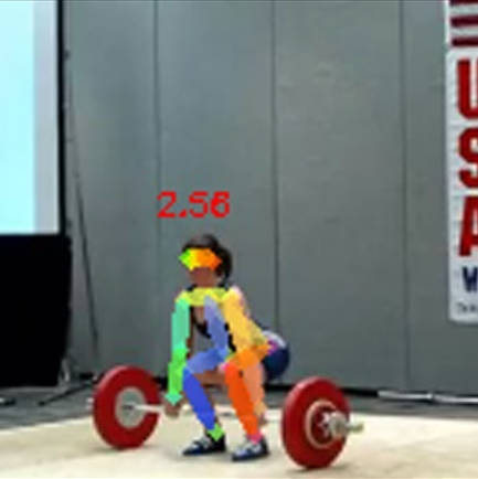
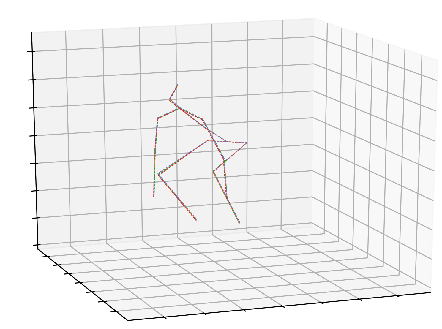
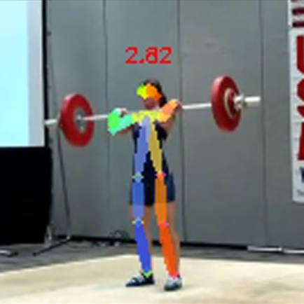
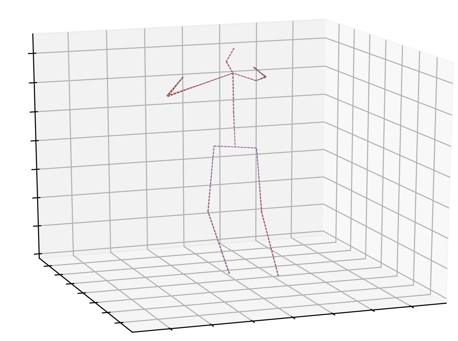
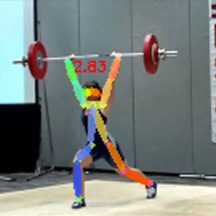
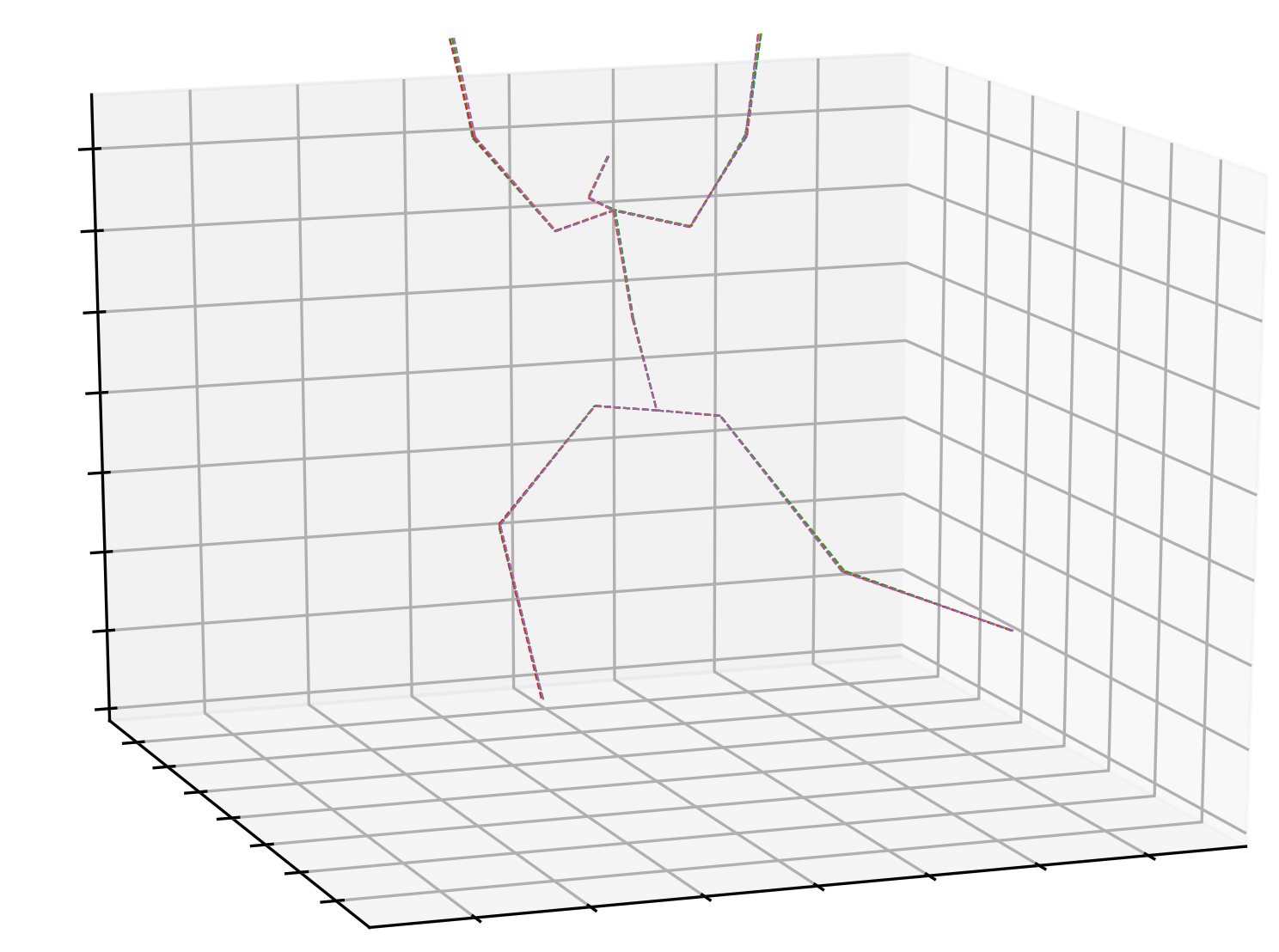
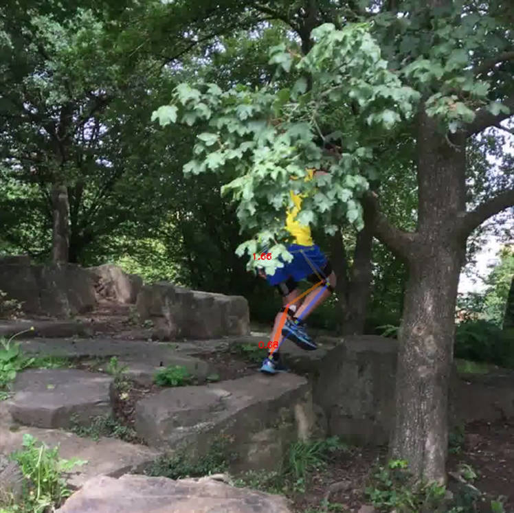
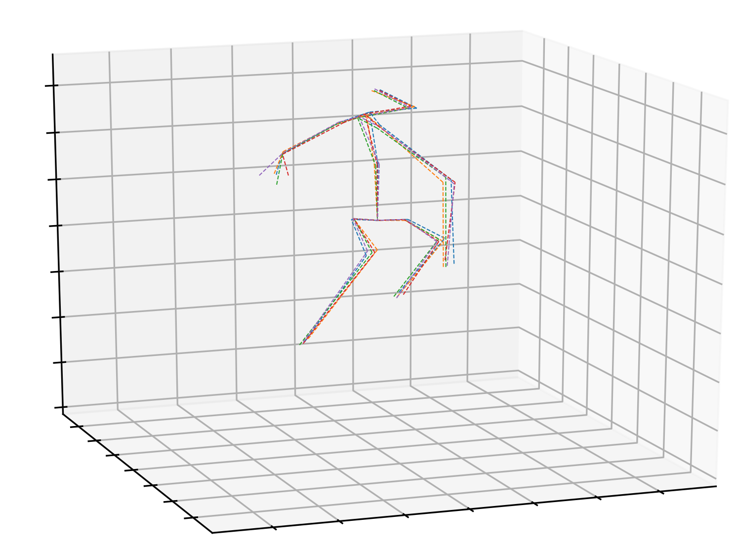
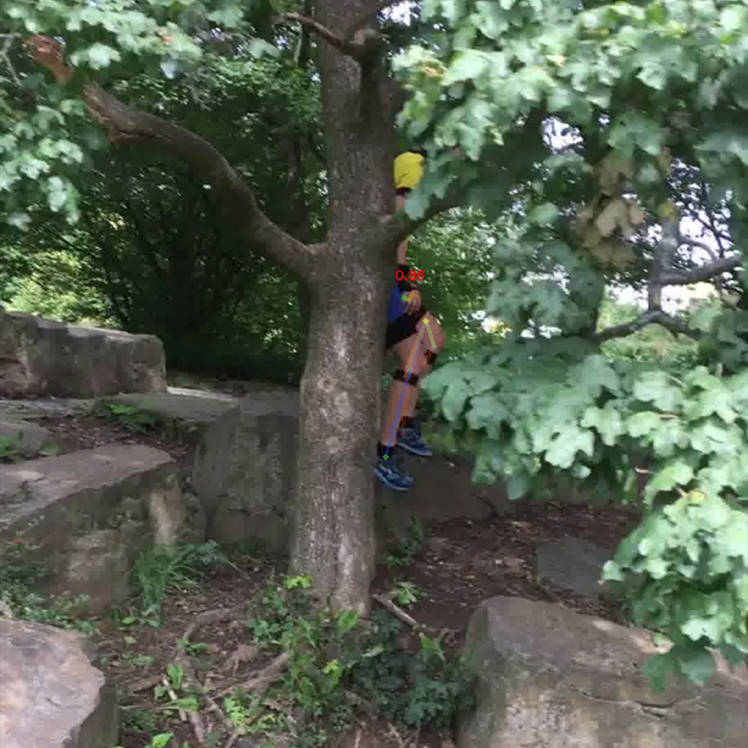
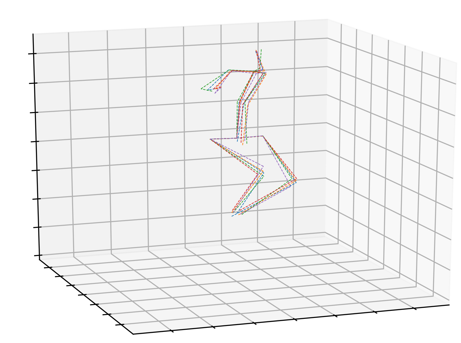
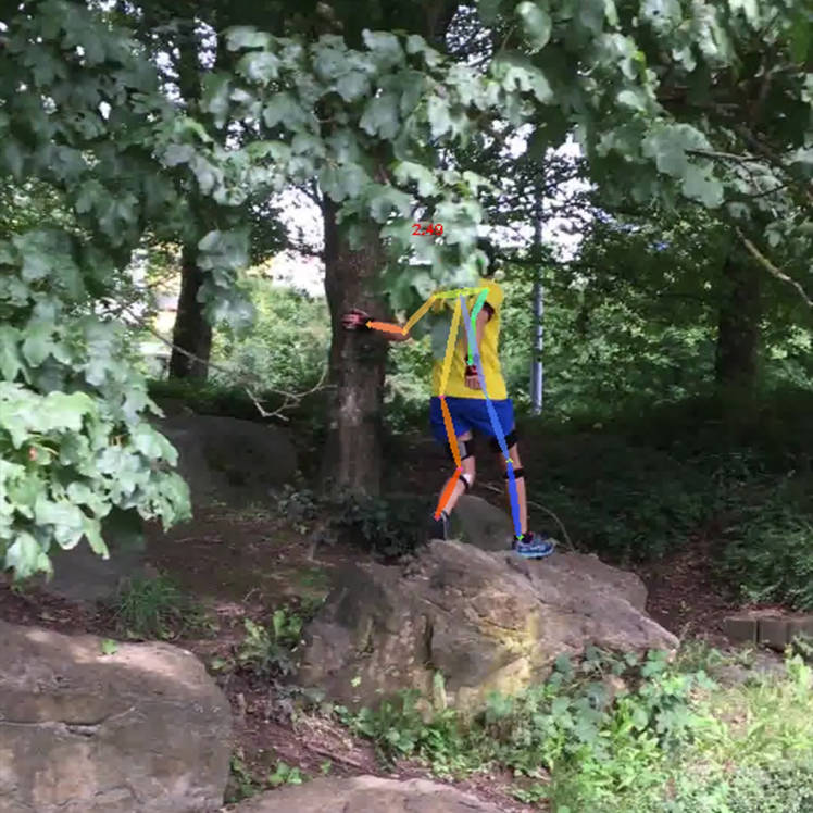
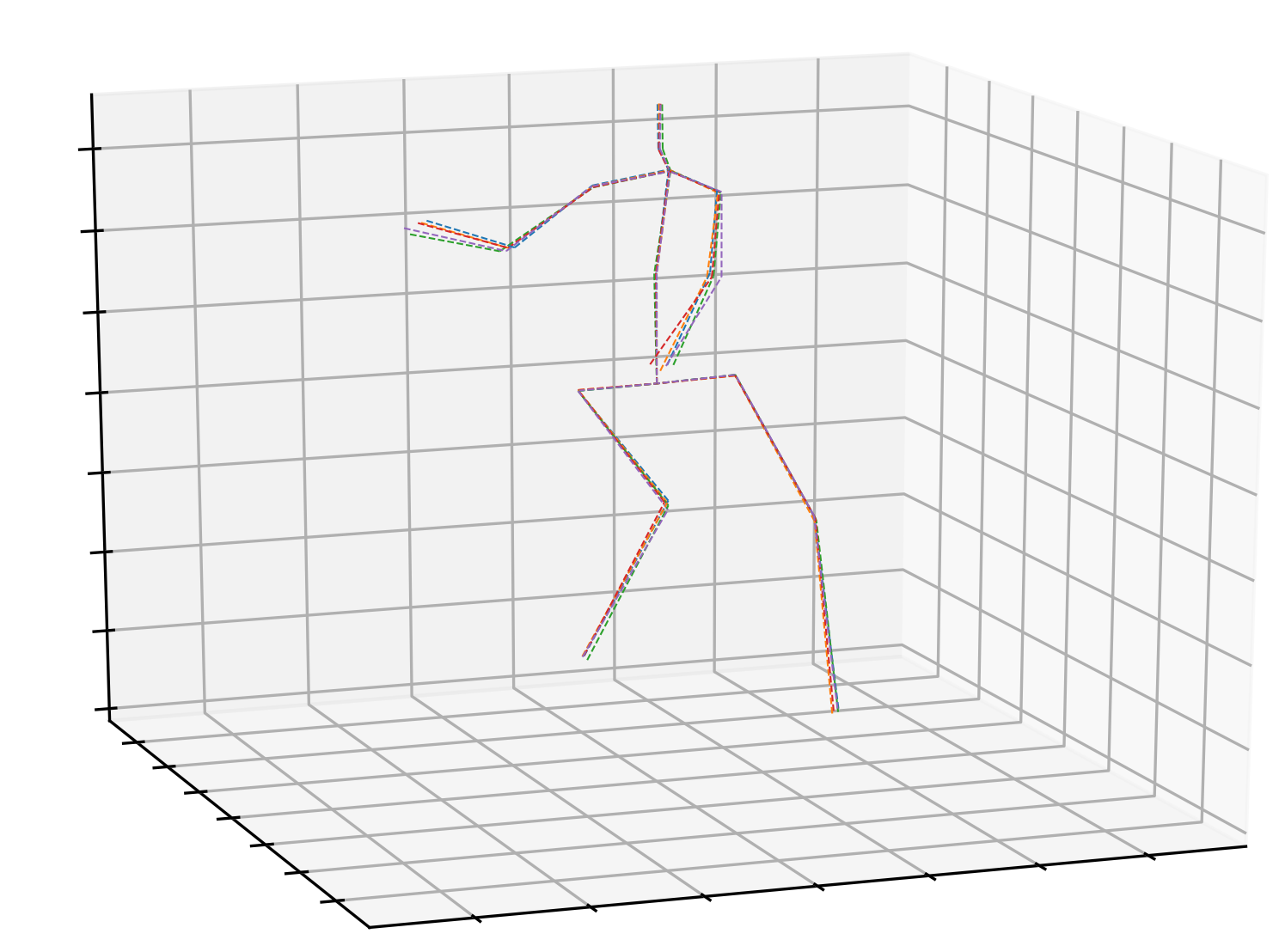
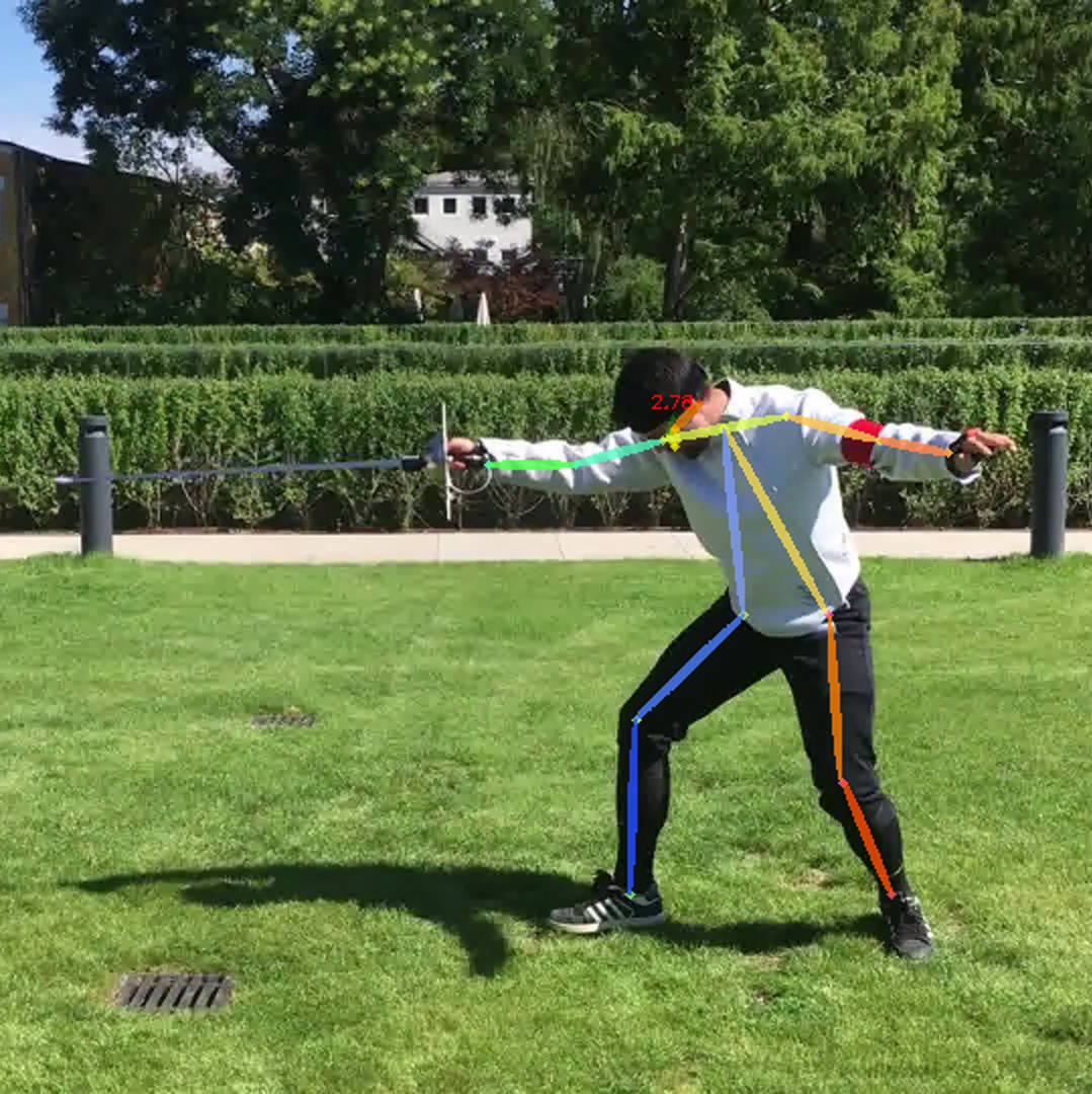
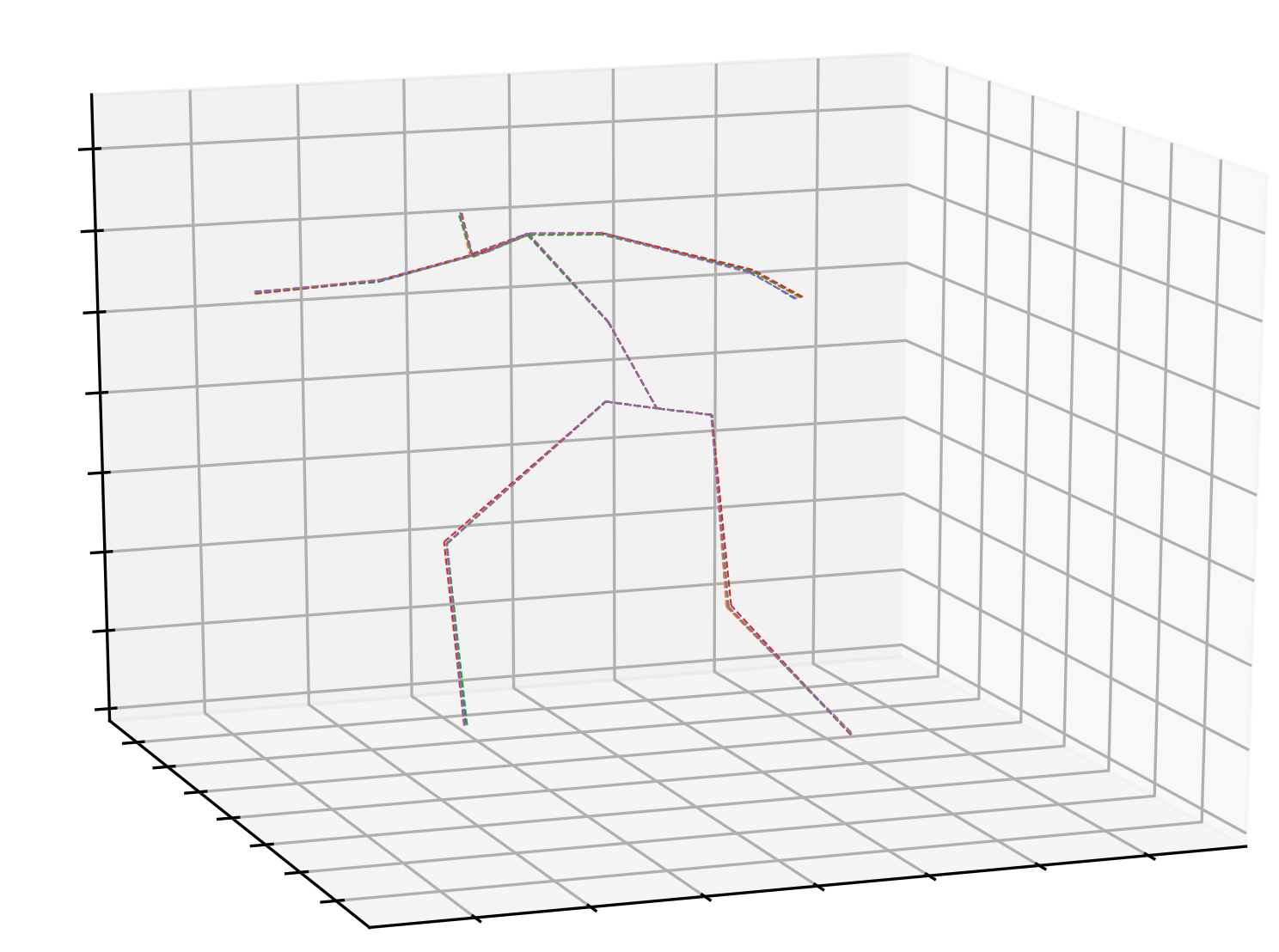
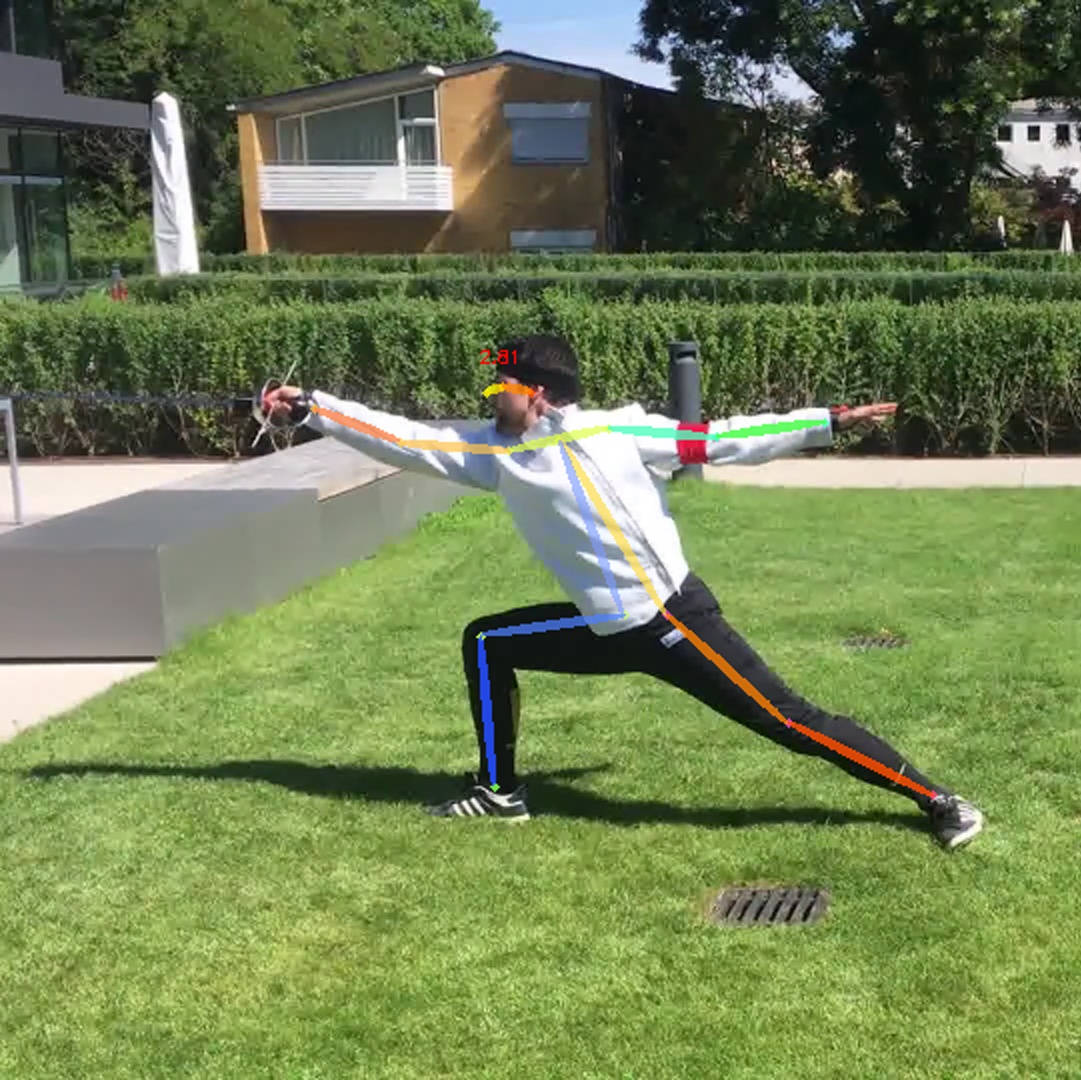
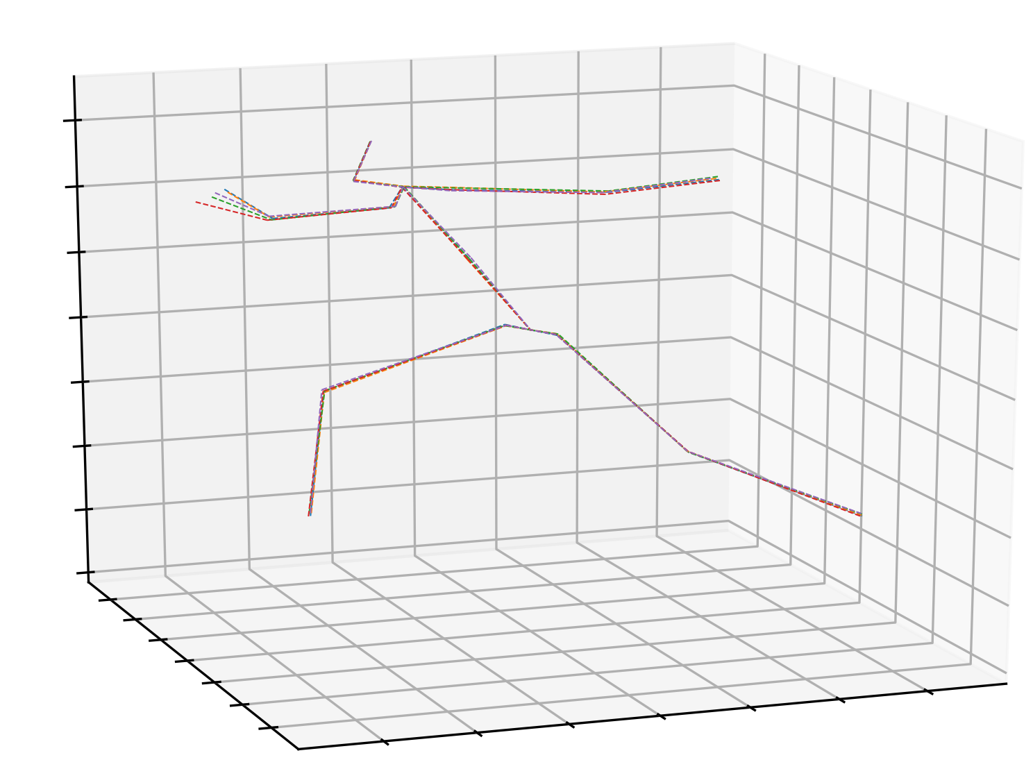
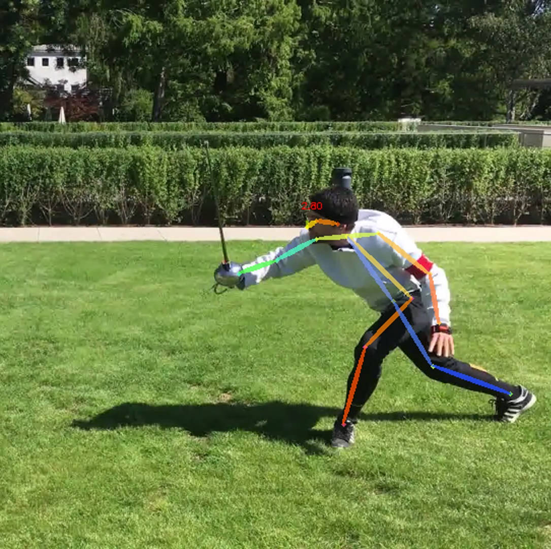
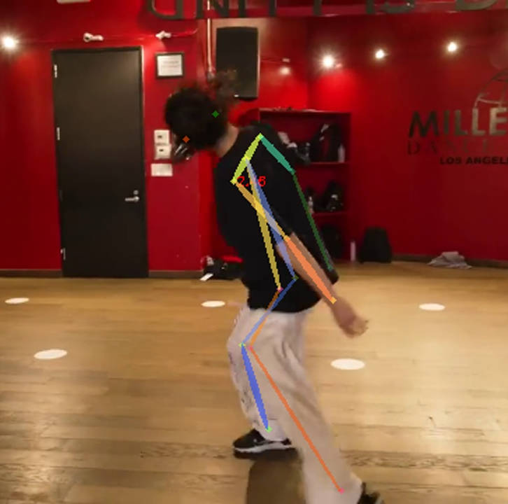
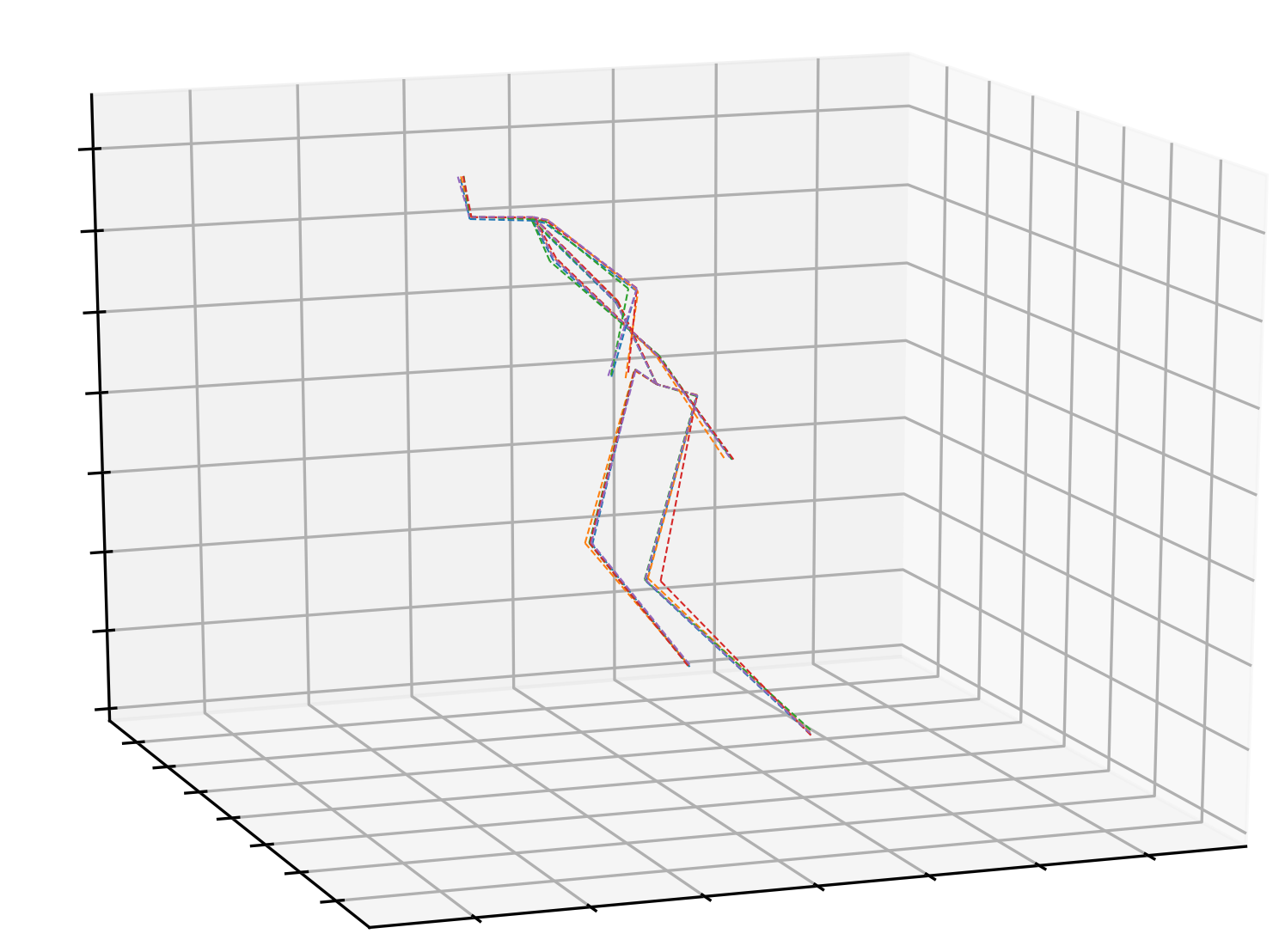
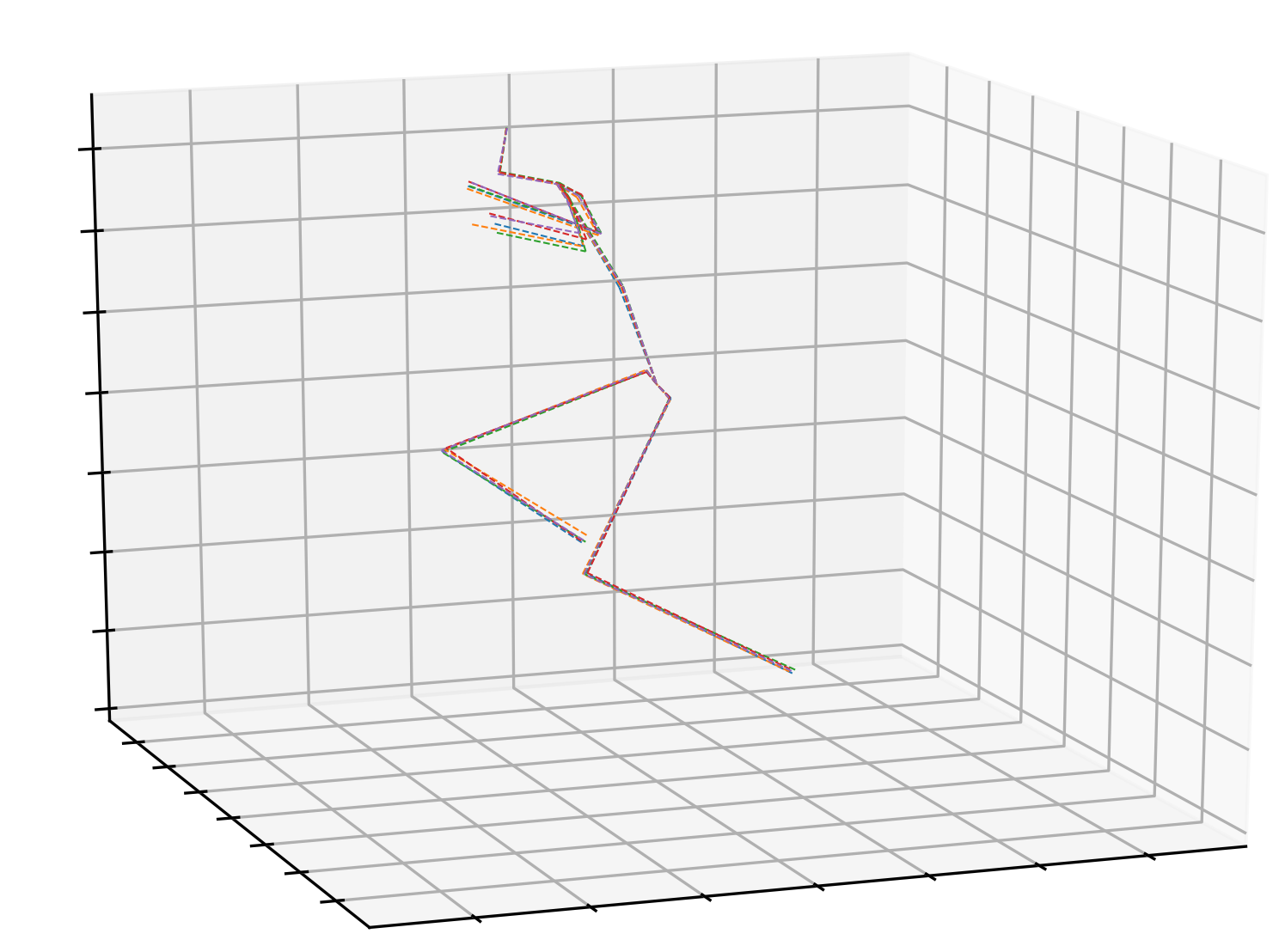
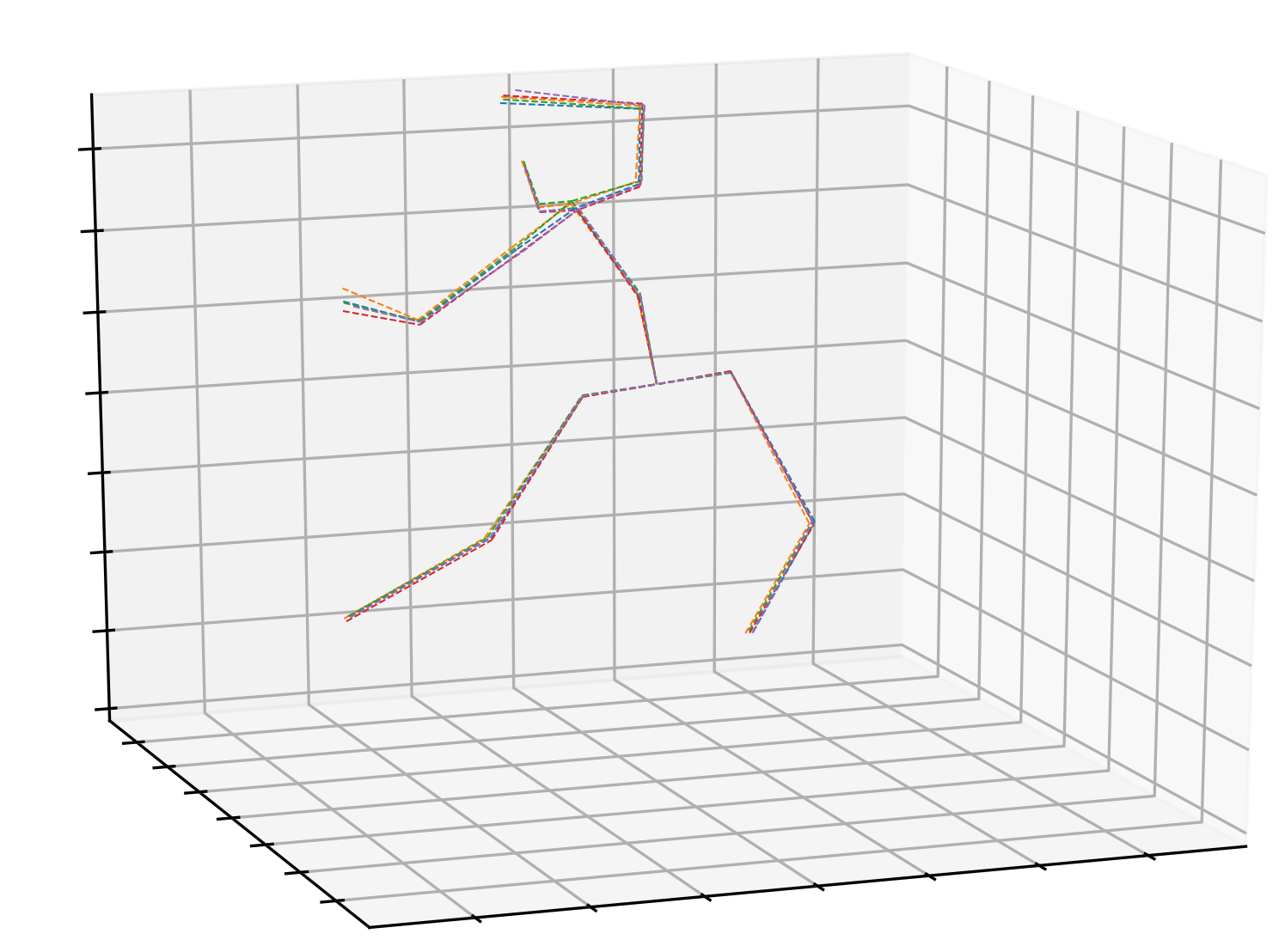
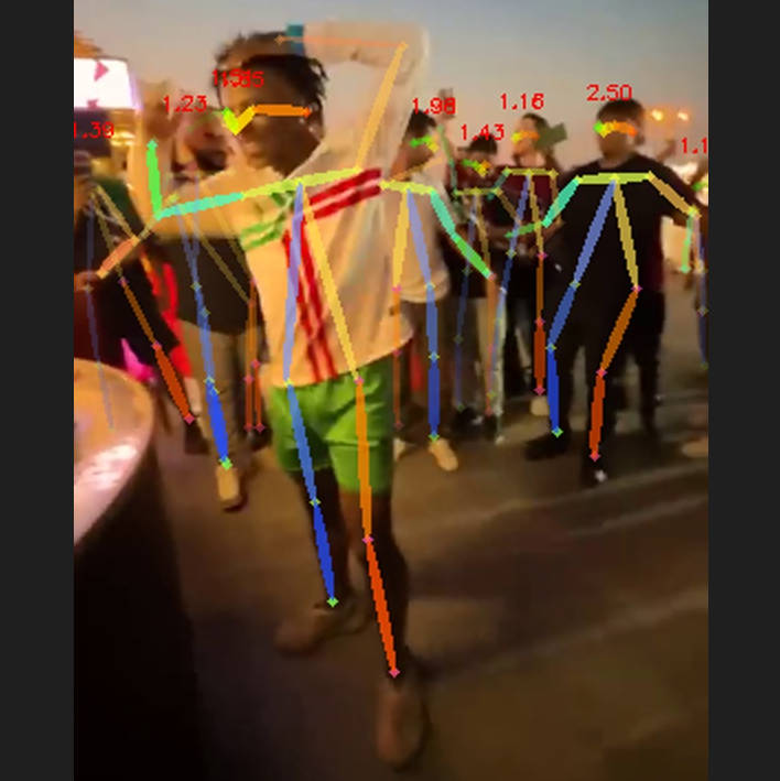
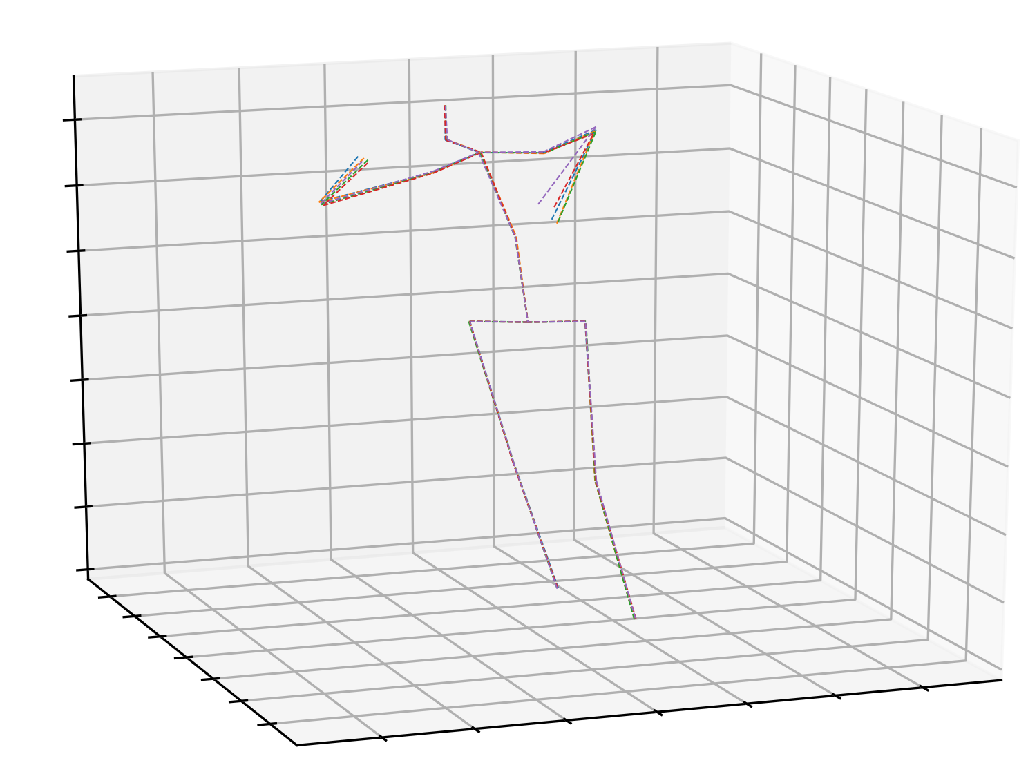
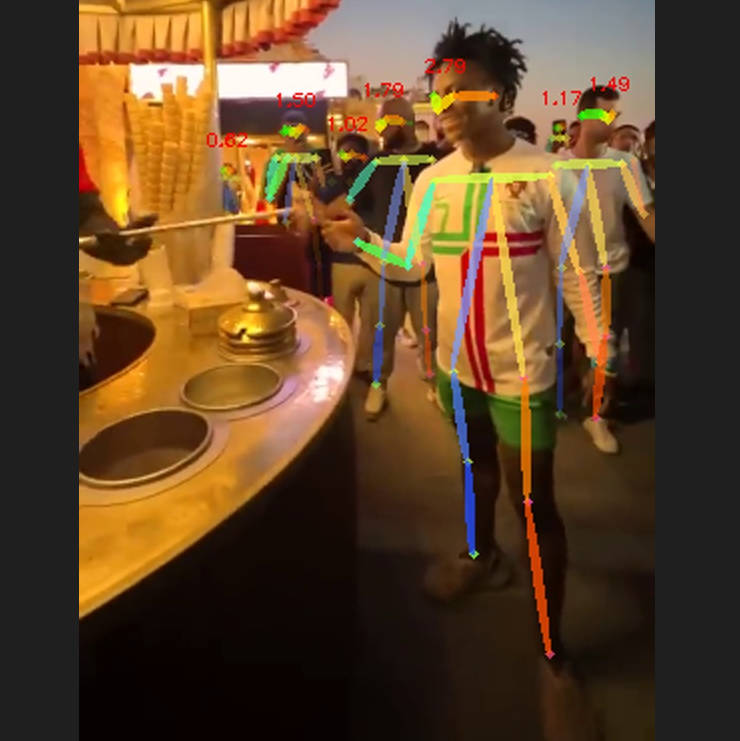
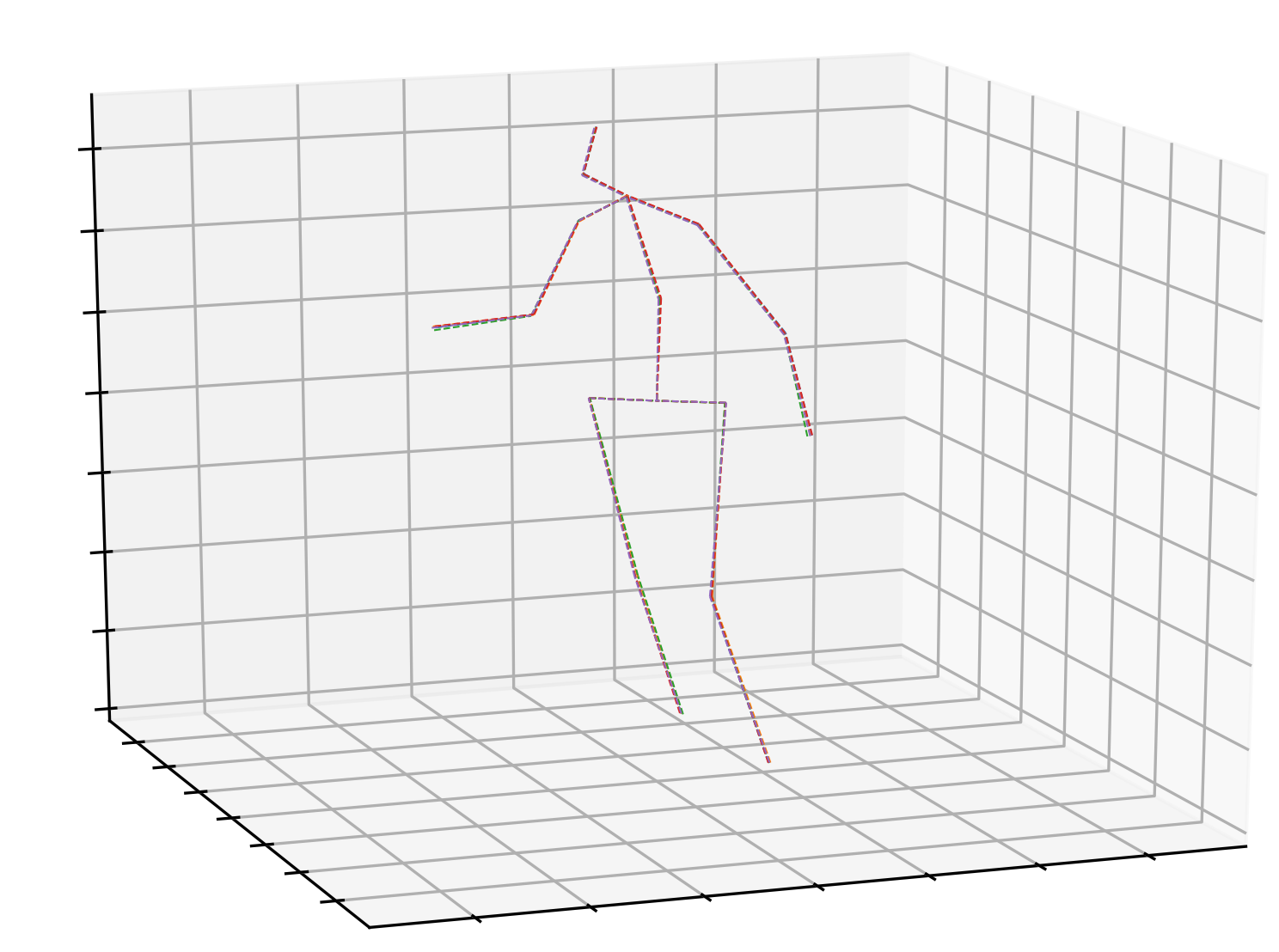
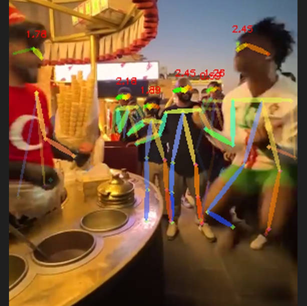
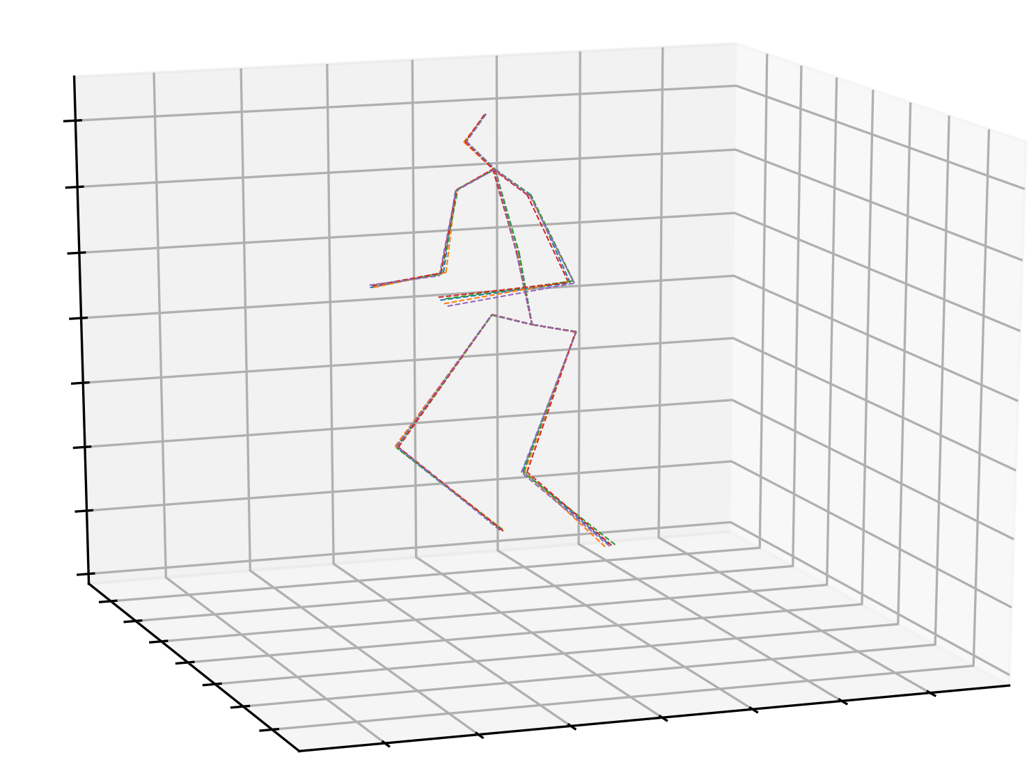
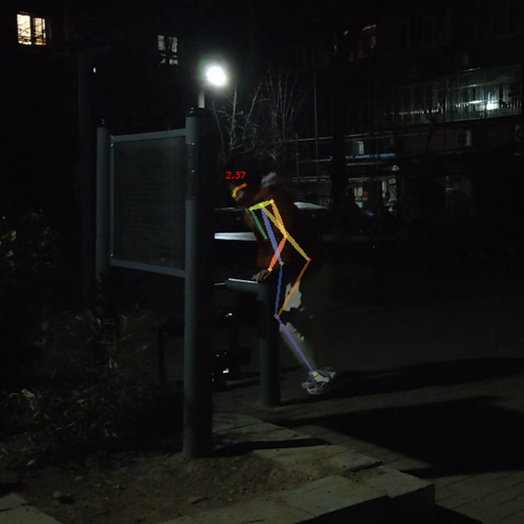
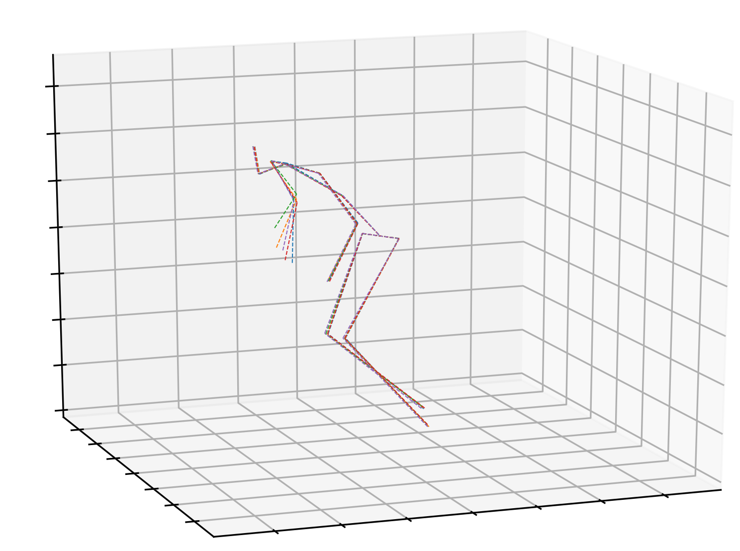
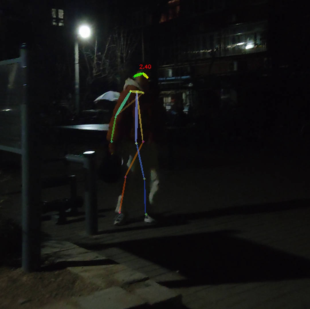
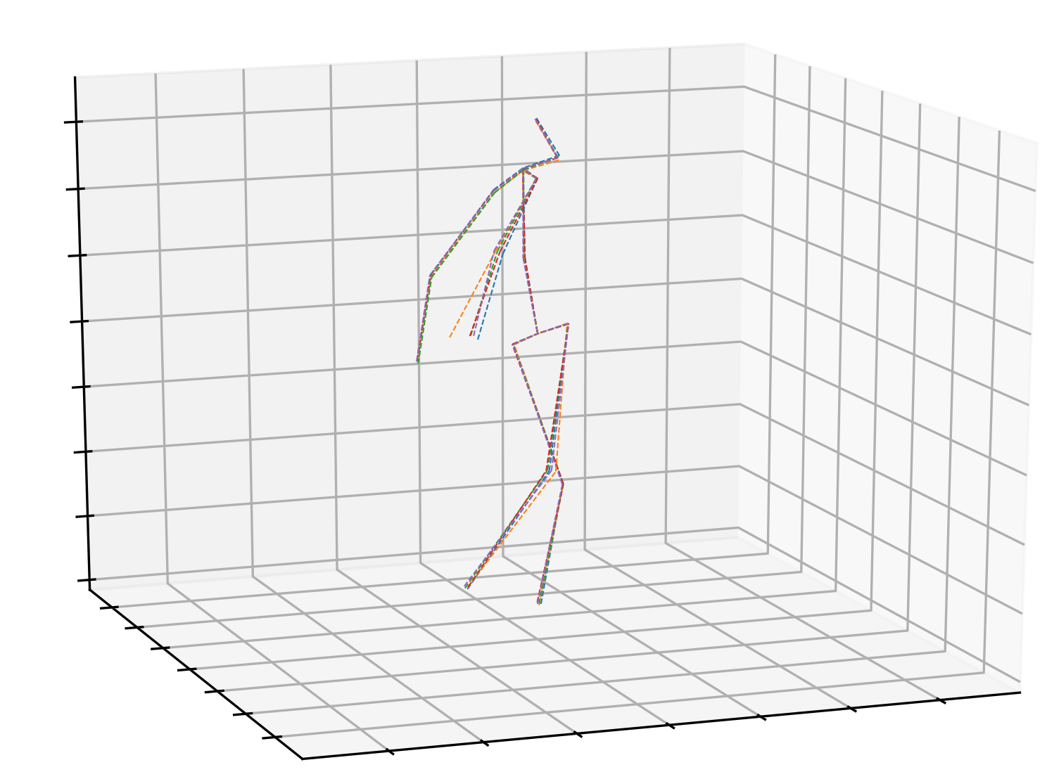
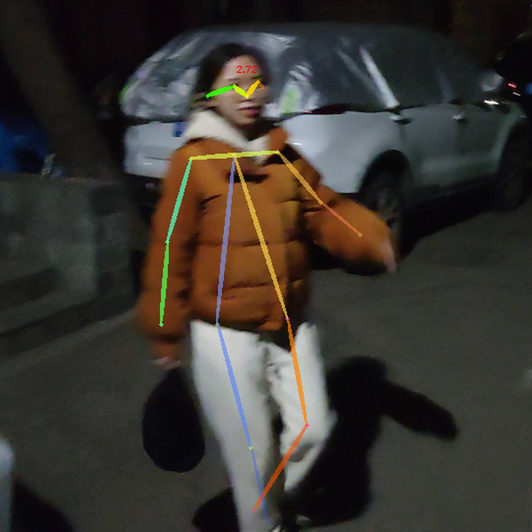
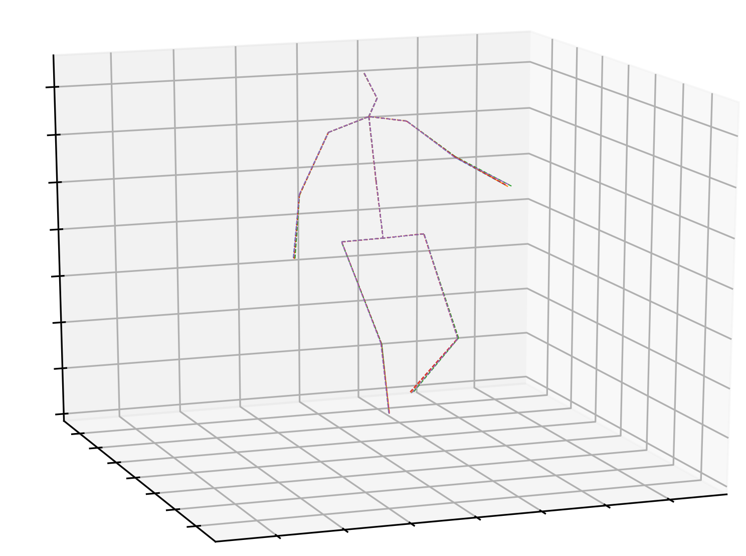
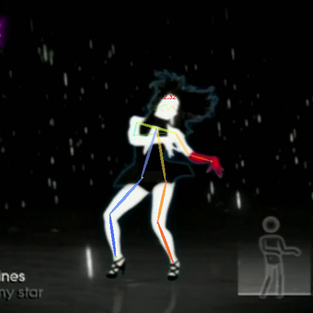
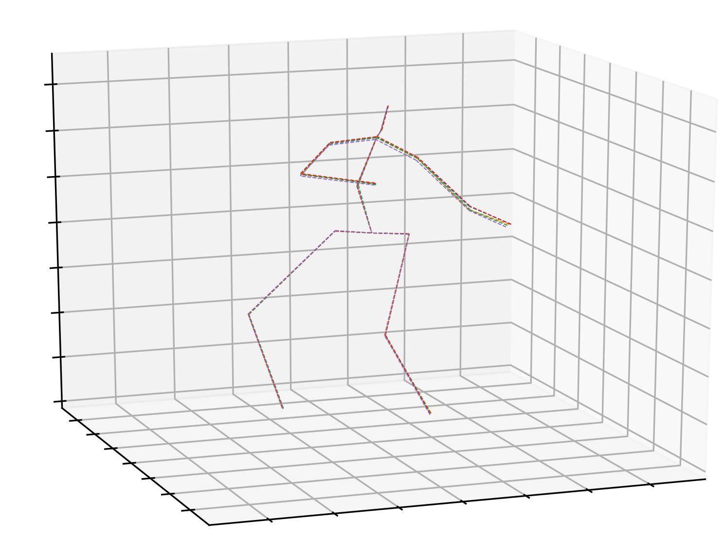
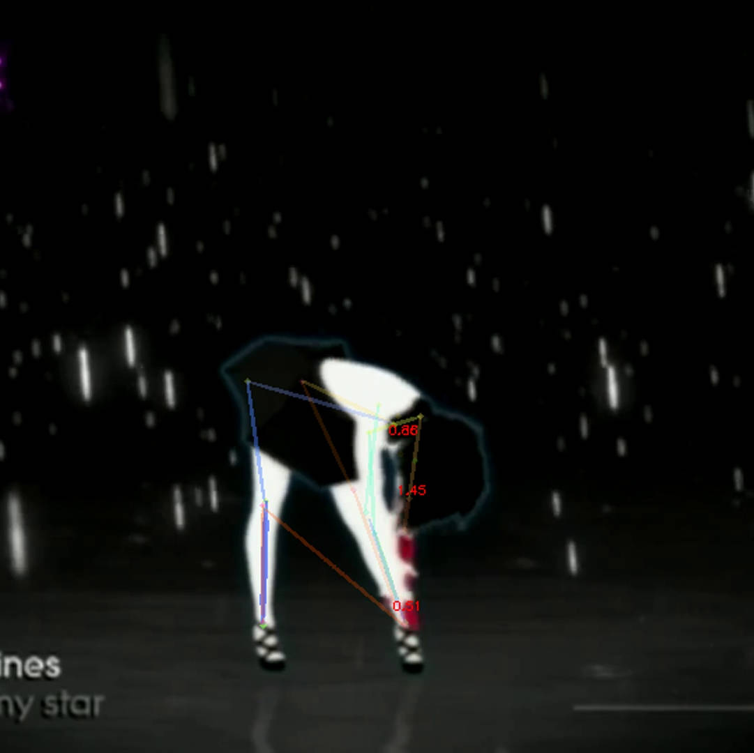
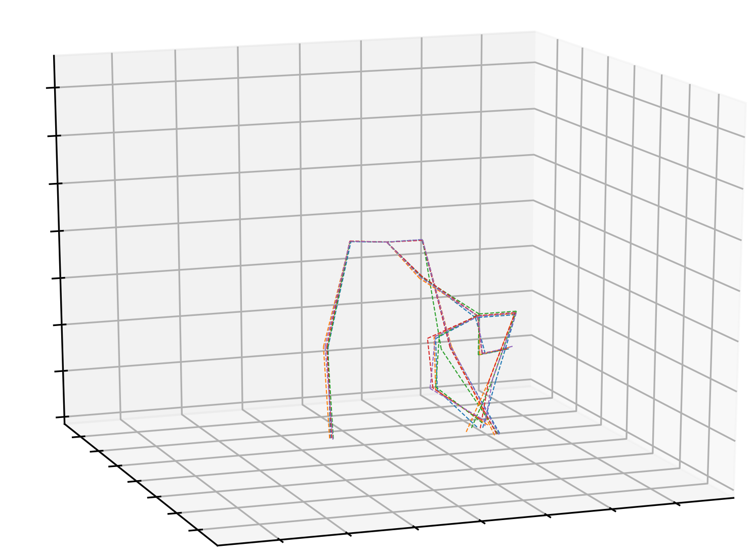
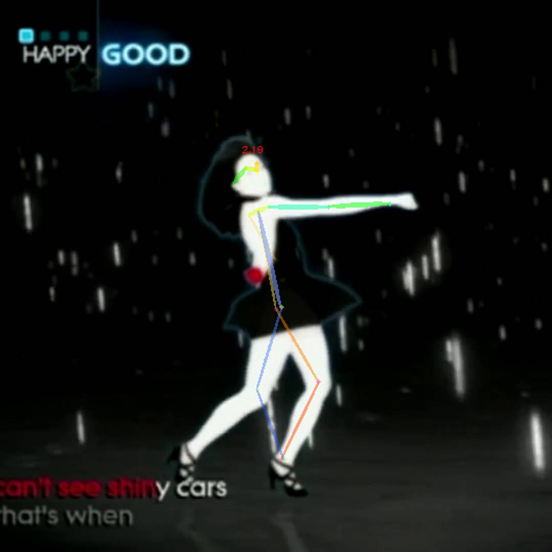
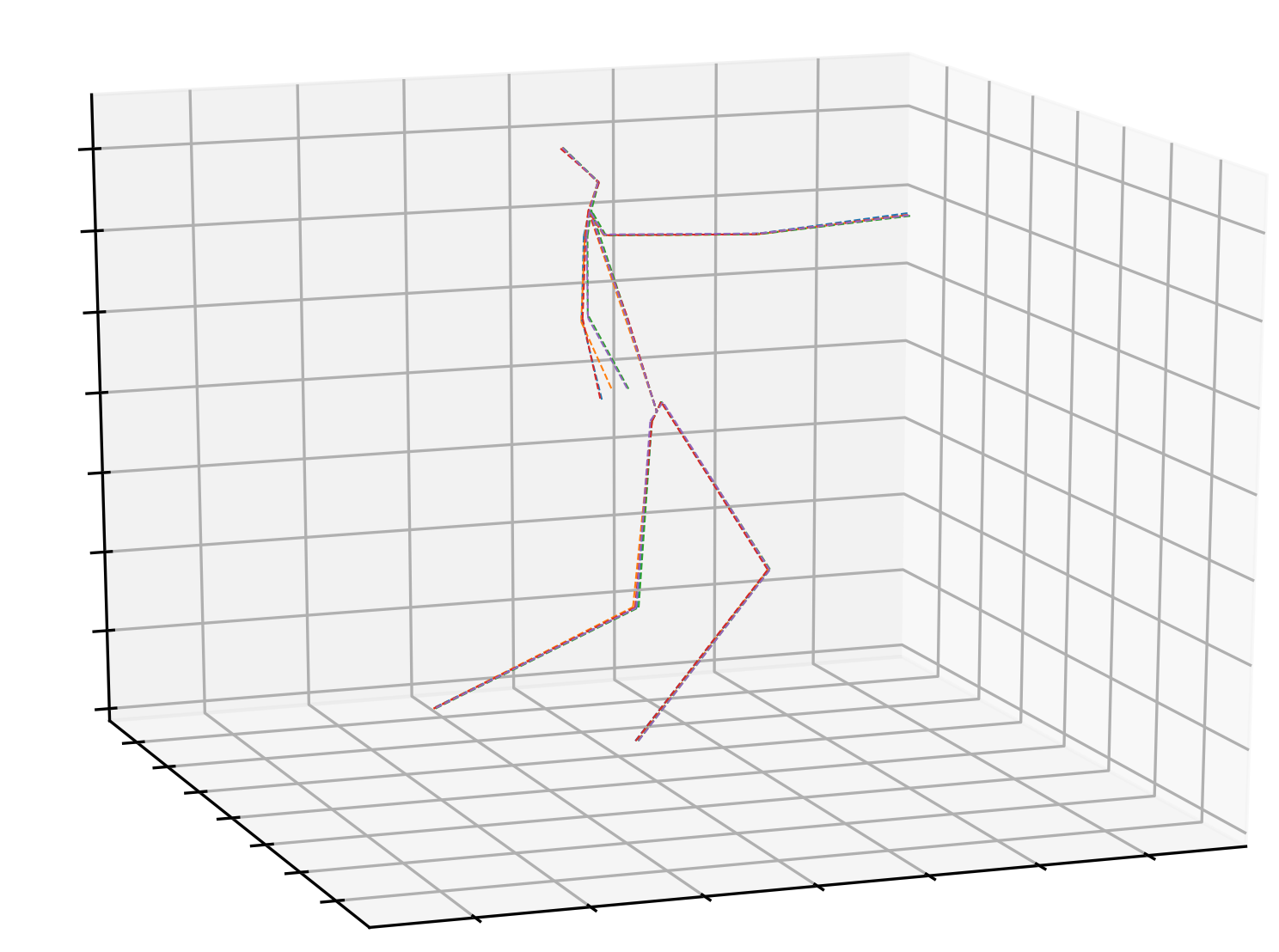
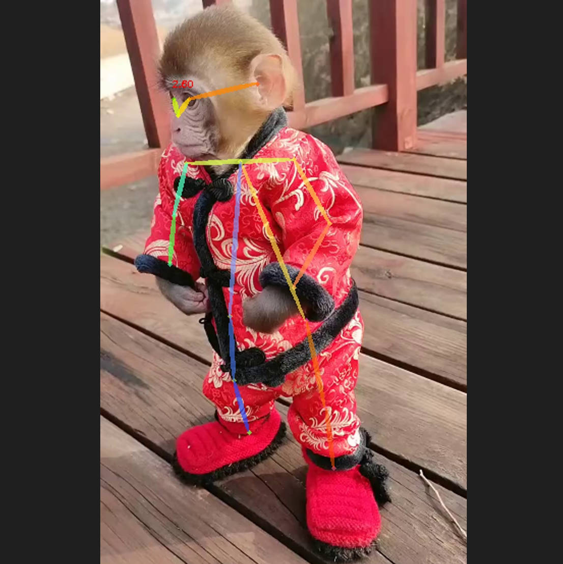
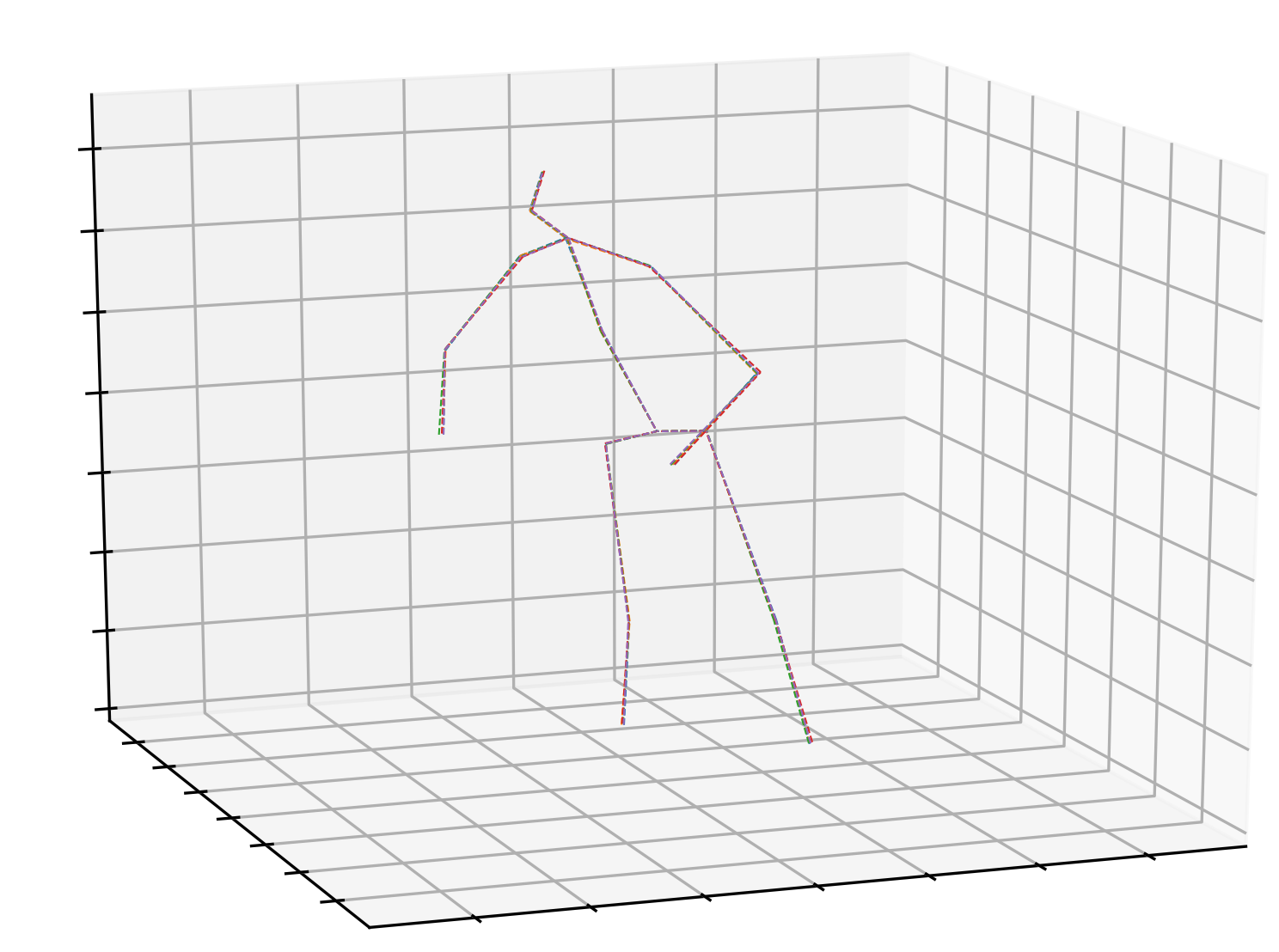
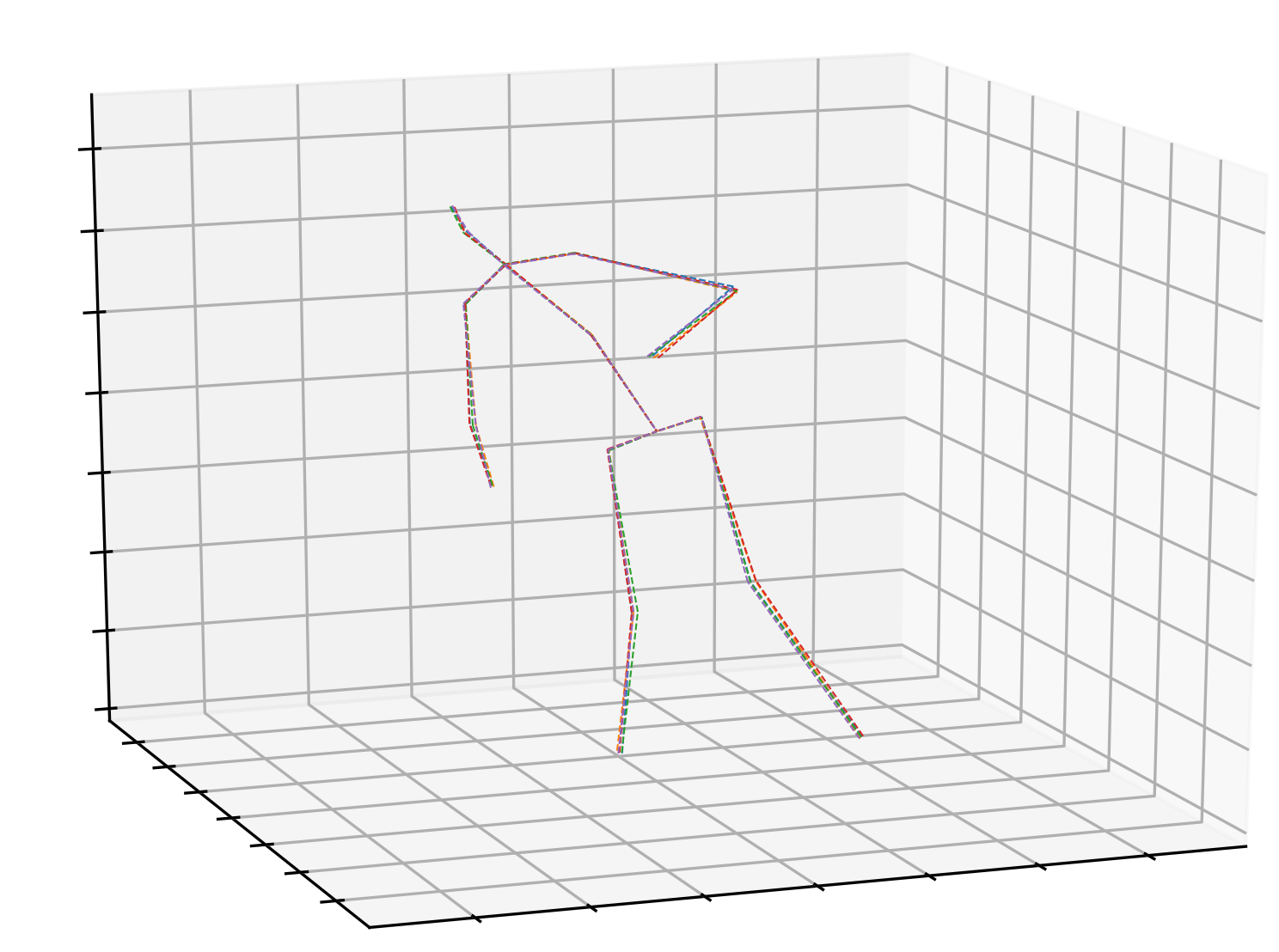
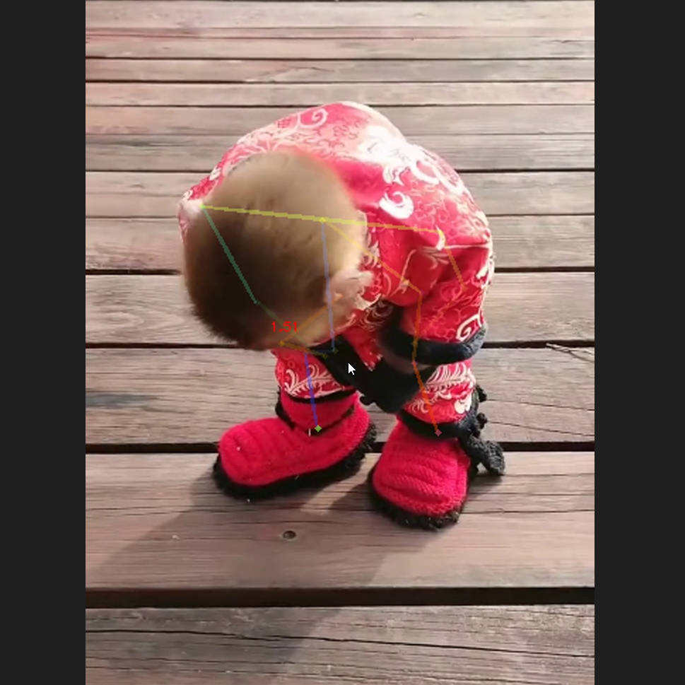
Figure 10: Qualitative results of the proposed method on in-the-wild videos. Dashed line: predicted 3D pose hypotheses. Each color represents an individual hypothesis. $H$=5, $K$=5

References

- [1] Omri Avrahami, Dani Lischinski, and Ohad Fried. Blended diffusion for text-driven editing of natural images. In Proceedings of the IEEE/CVF Conference on Computer Vision and Pattern Recognition, pages 18208–18218, 2022.
- [2] Dmitry Baranchuk, Ivan Rubachev, Andrey Voynov, Valentin Khrulkov, and Artem Babenko. Label-efficient semantic segmentation with diffusion models. arXiv preprint arXiv:2112.03126, 2021.
- [3] Georgios Batzolis, Jan Stanczuk, Carola-Bibiane Schönlieb, and Christian Etmann. Conditional image generation with score-based diffusion models. arXiv preprint arXiv:2111.13606, 2021.
- [4] Christopher M Bishop. Mixture density networks. 1994.
- [5] Emmanuel Asiedu Brempong, Simon Kornblith, Ting Chen, Niki Parmar, Matthias Minderer, and Mohammad Norouzi. Denoising pretraining for semantic segmentation. In Proceedings of the IEEE/CVF Conference on Computer Vision and Pattern Recognition, pages 4175–4186, 2022.
- [6] Zhe Cao, Tomas Simon, Shih-En Wei, and Yaser Sheikh. Realtime multi-person 2d pose estimation using part affinity fields. In Proceedings of the IEEE conference on computer vision and pattern recognition, pages 7291–7299, 2017.
- [7] Ching-Hang Chen, Ambrish Tyagi, Amit Agrawal, Dylan Drover, Rohith Mv, Stefan Stojanov, and James M Rehg. Unsupervised 3d pose estimation with geometric self-supervision. In Proceedings of the IEEE/CVF Conference on Computer Vision and Pattern Recognition, pages 5714–5724, 2019.
- [8] Shoufa Chen, Peize Sun, Yibing Song, and Ping Luo. Diffusiondet: Diffusion model for object detection. arXiv preprint arXiv:2211.09788, 2022.
- [9] Tianlang Chen, Chen Fang, Xiaohui Shen, Yiheng Zhu, Zhili Chen, and Jiebo Luo. Anatomy-aware 3d human pose estimation with bone-based pose decomposition. IEEE Transactions on Circuits and Systems for Video Technology, 2021.
- [10] Ting Chen, Lala Li, Saurabh Saxena, Geoffrey Hinton, and David J Fleet. A generalist framework for panoptic segmentation of images and videos. arXiv preprint arXiv:2210.06366, 2022.
- [11] Yilun Chen, Zhicheng Wang, Yuxiang Peng, Zhiqiang Zhang, Gang Yu, and Jian Sun. Cascaded pyramid network for multi-person pose estimation. In Proceedings of the IEEE conference on computer vision and pattern recognition, pages 7103–7112, 2018.
- [12] Yu Cheng, Bo Yang, Bo Wang, Wending Yan, and Robby T Tan. Occlusion-aware networks for 3d human pose estimation in video. In Proceedings of the IEEE/CVF international conference on computer vision, pages 723–732, 2019.
- [13] Hanbyel Cho, Yooshin Cho, Jaemyung Yu, and Junmo Kim. Camera distortion-aware 3d human pose estimation in video with optimization-based meta-learning. In Proceedings of the IEEE/CVF International Conference on Computer Vision, pages 11169–11178, 2021.
- [14] Jeongjun Choi, Dongseok Shim, and H Jin Kim. Diffupose: Monocular 3d human pose estimation via denoising diffusion probabilistic model. arXiv preprint arXiv:2212.02796, 2022.
- [15] Hai Ci, Chunyu Wang, Xiaoxuan Ma, and Yizhou Wang. Optimizing network structure for 3d human pose estimation. In Proceedings of the IEEE/CVF International Conference on Computer Vision, pages 2262–2271, 2019.
- [16] Wan-Cyuan Fan, Yen-Chun Chen, DongDong Chen, Yu Cheng, Lu Yuan, and Yu-Chiang Frank Wang. Frido: Feature pyramid diffusion for complex scene image synthesis. arXiv preprint arXiv:2208.13753, 2022.
- [17] Hao-Shu Fang, Shuqin Xie, Yu-Wing Tai, and Cewu Lu. Rmpe: Regional multi-person pose estimation. In Proceedings of the IEEE international conference on computer vision, pages 2334–2343, 2017.
- [18] Jia Gong, Lin Geng Foo, Zhipeng Fan, Qiuhong Ke, Hossein Rahmani, and Jun Liu. Diffpose: Toward more reliable 3d pose estimation. In Proceedings of the IEEE/CVF Conference on Computer Vision and Pattern Recognition, pages 13041–13051, 2023.
- [19] Ian Goodfellow, Jean Pouget-Abadie, Mehdi Mirza, Bing Xu, David Warde-Farley, Sherjil Ozair, Aaron Courville, and Yoshua Bengio. Generative adversarial networks. Communications of the ACM, 63(11):139–144, 2020.
- [20] Jonathan Ho, Ajay Jain, and Pieter Abbeel. Denoising diffusion probabilistic models. Advances in Neural Information Processing Systems, 33:6840–6851, 2020.
- [21] Jonathan Ho, Chitwan Saharia, William Chan, David J Fleet, Mohammad Norouzi, and Tim Salimans. Cascaded diffusion models for high fidelity image generation. J. Mach. Learn. Res., 23(47):1–33, 2022.
- [22] Karl Holmquist and Bastian Wandt. Diffpose: Multi-hypothesis human pose estimation using diffusion models. arXiv preprint arXiv:2211.16487, 2022.
- [23] Wenbo Hu, Changgong Zhang, Fangneng Zhan, Lei Zhang, and Tien-Tsin Wong. Conditional directed graph convolution for 3d human pose estimation. In Proceedings of the 29th ACM International Conference on Multimedia, pages 602–611, 2021.
- [24] Rongjie Huang, Zhou Zhao, Huadai Liu, Jinglin Liu, Chenye Cui, and Yi Ren. Prodiff: Progressive fast diffusion model for high-quality text-to-speech. In Proceedings of the 30th ACM International Conference on Multimedia, pages 2595–2605, 2022.
- [25] Catalin Ionescu, Dragos Papava, Vlad Olaru, and Cristian Sminchisescu. Human3. 6m: Large scale datasets and predictive methods for 3d human sensing in natural environments. IEEE transactions on pattern analysis and machine intelligence, 36(7):1325–1339, 2013.
- [26] Ehsan Jahangiri and Alan L Yuille. Generating multiple diverse hypotheses for human 3d pose consistent with 2d joint detections. In Proceedings of the IEEE International Conference on Computer Vision Workshops, pages 805–814, 2017.
- [27] H. Jhuang, J. Gall, S. Zuffi, C. Schmid, and M. J. Black. Towards understanding action recognition. In International Conf. on Computer Vision (ICCV), pages 3192–3199, Dec. 2013.
- [28] Jaehyeong Jo, Seul Lee, and Sung Ju Hwang. Score-based generative modeling of graphs via the system of stochastic differential equations. In International Conference on Machine Learning, pages 10362–10383. PMLR, 2022.
- [29] Sungwon Kim, Heeseung Kim, and Sungroh Yoon. Guided-tts 2: A diffusion model for high-quality adaptive text-to-speech with untranscribed data. arXiv preprint arXiv:2205.15370, 2022.
- [30] Jogendra Nath Kundu, Siddharth Seth, MV Rahul, Mugalodi Rakesh, Venkatesh Babu Radhakrishnan, and Anirban Chakraborty. Kinematic-structure-preserved representation for unsupervised 3d human pose estimation. In Proceedings of the AAAI Conference on Artificial Intelligence, volume 34, pages 11312–11319, 2020.
- [31] Mun Wai Lee and Isaac Cohen. Proposal maps driven mcmc for estimating human body pose in static images. In Proceedings of the 2004 IEEE Computer Society Conference on Computer Vision and Pattern Recognition, 2004. CVPR 2004., volume 2, pages II–II. IEEE, 2004.
- [32] Alon Levkovitch, Eliya Nachmani, and Lior Wolf. Zero-shot voice conditioning for denoising diffusion tts models. arXiv preprint arXiv:2206.02246, 2022.
- [33] Chen Li and Gim Hee Lee. Generating multiple hypotheses for 3d human pose estimation with mixture density network. In Proceedings of the IEEE/CVF conference on computer vision and pattern recognition, pages 9887–9895, 2019.
- [34] Chen Li and Gim Hee Lee. Weakly supervised generative network for multiple 3d human pose hypotheses. BMVC, 2020.
- [35] Wenhao Li, Hong Liu, Runwei Ding, Mengyuan Liu, Pichao Wang, and Wenming Yang. Exploiting temporal contexts with strided transformer for 3d human pose estimation. IEEE Transactions on Multimedia, 2022.
- [36] Wenhao Li, Hong Liu, Hao Tang, Pichao Wang, and Luc Van Gool. Mhformer: Multi-hypothesis transformer for 3d human pose estimation. In Proceedings of the IEEE/CVF Conference on Computer Vision and Pattern Recognition, pages 13147–13156, 2022.
- [37] Ruixu Liu, Ju Shen, He Wang, Chen Chen, Sen-ching Cheung, and Vijayan Asari. Attention mechanism exploits temporal contexts: Real-time 3d human pose reconstruction. In Proceedings of the IEEE/CVF Conference on Computer Vision and Pattern Recognition, pages 5064–5073, 2020.
- [38] Ilya Loshchilov and Frank Hutter. Decoupled weight decay regularization. arXiv preprint arXiv:1711.05101, 2017.
- [39] Julieta Martinez, Rayat Hossain, Javier Romero, and James J Little. A simple yet effective baseline for 3d human pose estimation. In Proceedings of the IEEE International Conference on Computer Vision, pages 2640–2649, 2017.
- [40] Dushyant Mehta, Helge Rhodin, Dan Casas, Pascal Fua, Oleksandr Sotnychenko, Weipeng Xu, and Christian Theobalt. Monocular 3d human pose estimation in the wild using improved cnn supervision. In 2017 international conference on 3D vision (3DV), pages 506–516. IEEE, 2017.
- [41] Alex Nichol, Prafulla Dhariwal, Aditya Ramesh, Pranav Shyam, Pamela Mishkin, Bob McGrew, Ilya Sutskever, and Mark Chen. Glide: Towards photorealistic image generation and editing with text-guided diffusion models. arXiv preprint arXiv:2112.10741, 2021.
- [42] Alexander Quinn Nichol and Prafulla Dhariwal. Improved denoising diffusion probabilistic models. In International Conference on Machine Learning, pages 8162–8171. PMLR, 2021.
- [43] Chenhao Niu, Yang Song, Jiaming Song, Shengjia Zhao, Aditya Grover, and Stefano Ermon. Permutation invariant graph generation via score-based generative modeling. In International Conference on Artificial Intelligence and Statistics, pages 4474–4484. PMLR, 2020.
- [44] Tuomas Oikarinen, Daniel Hannah, and Sohrob Kazerounian. Graphmdn: Leveraging graph structure and deep learning to solve inverse problems. In 2021 International Joint Conference on Neural Networks (IJCNN), pages 1–9. IEEE, 2021.
- [45] Adam Paszke, Sam Gross, Francisco Massa, Adam Lerer, James Bradbury, Gregory Chanan, Trevor Killeen, Zeming Lin, Natalia Gimelshein, Luca Antiga, et al. Pytorch: An imperative style, high-performance deep learning library. Advances in neural information processing systems, 32, 2019.
- [46] Dario Pavllo, Christoph Feichtenhofer, David Grangier, and Michael Auli. 3d human pose estimation in video with temporal convolutions and semi-supervised training. In Proceedings of the IEEE/CVF Conference on Computer Vision and Pattern Recognition, pages 7753–7762, 2019.
- [47] Danilo Rezende and Shakir Mohamed. Variational inference with normalizing flows. In International conference on machine learning, pages 1530–1538. PMLR, 2015.
- [48] Robin Rombach, Andreas Blattmann, Dominik Lorenz, Patrick Esser, and Björn Ommer. High-resolution image synthesis with latent diffusion models. In Proceedings of the IEEE/CVF Conference on Computer Vision and Pattern Recognition, pages 10684–10695, 2022.
- [49] Chitwan Saharia, William Chan, Huiwen Chang, Chris Lee, Jonathan Ho, Tim Salimans, David Fleet, and Mohammad Norouzi. Palette: Image-to-image diffusion models. In ACM SIGGRAPH 2022 Conference Proceedings, pages 1–10, 2022.
- [50] Chitwan Saharia, Jonathan Ho, William Chan, Tim Salimans, David J Fleet, and Mohammad Norouzi. Image super-resolution via iterative refinement. IEEE Transactions on Pattern Analysis and Machine Intelligence, 2022.
- [51] Wenkang Shan, Zhenhua Liu, Xinfeng Zhang, Shanshe Wang, Siwei Ma, and Wen Gao. P-stmo: Pre-trained spatial temporal many-to-one model for 3d human pose estimation. In Computer Vision–ECCV 2022: 17th European Conference, Tel Aviv, Israel, October 23–27, 2022, Proceedings, Part V, pages 461–478. Springer, 2022.
- [52] Wenkang Shan, Haopeng Lu, Shanshe Wang, Xinfeng Zhang, and Wen Gao. Improving robustness and accuracy via relative information encoding in 3d human pose estimation. In Proceedings of the 29th ACM International Conference on Multimedia, pages 3446–3454, 2021.
- [53] Saurabh Sharma, Pavan Teja Varigonda, Prashast Bindal, Abhishek Sharma, and Arjun Jain. Monocular 3d human pose estimation by generation and ordinal ranking. In Proceedings of the IEEE/CVF international conference on computer vision, pages 2325–2334, 2019.
- [54] Edgar Simo-Serra, Arnau Ramisa, Guillem Alenya, Carme Torras, and Francesc Moreno-Noguer. Single image 3d human pose estimation from noisy observations. In 2012 IEEE Conference on Computer Vision and Pattern Recognition, pages 2673–2680. IEEE, 2012.
- [55] Jascha Sohl-Dickstein, Eric Weiss, Niru Maheswaranathan, and Surya Ganguli. Deep unsupervised learning using nonequilibrium thermodynamics. In International Conference on Machine Learning, pages 2256–2265. PMLR, 2015.
- [56] Kihyuk Sohn, Honglak Lee, and Xinchen Yan. Learning structured output representation using deep conditional generative models. Advances in neural information processing systems, 28, 2015.
- [57] Jiaming Song, Chenlin Meng, and Stefano Ermon. Denoising diffusion implicit models. arXiv preprint arXiv:2010.02502, 2020.
- [58] Ashish Vaswani, Noam Shazeer, Niki Parmar, Jakob Uszkoreit, Llion Jones, Aidan N Gomez, Łukasz Kaiser, and Illia Polosukhin. Attention is all you need. In Advances in neural information processing systems, pages 5998–6008, 2017.
- [59] Clement Vignac, Igor Krawczuk, Antoine Siraudin, Bohan Wang, Volkan Cevher, and Pascal Frossard. Digress: Discrete denoising diffusion for graph generation. arXiv preprint arXiv:2209.14734, 2022.
- [60] Timo von Marcard, Roberto Henschel, Michael Black, Bodo Rosenhahn, and Gerard Pons-Moll. Recovering accurate 3d human pose in the wild using imus and a moving camera. In European Conference on Computer Vision (ECCV), sep 2018.
- [61] Bastian Wandt and Bodo Rosenhahn. Repnet: Weakly supervised training of an adversarial reprojection network for 3d human pose estimation. In Proceedings of the IEEE/CVF conference on computer vision and pattern recognition, pages 7782–7791, 2019.
- [62] Jingbo Wang, Sijie Yan, Yuanjun Xiong, and Dahua Lin. Motion guided 3d pose estimation from videos. In European Conference on Computer Vision, pages 764–780. Springer, 2020.
- [63] Tom Wehrbein, Marco Rudolph, Bodo Rosenhahn, and Bastian Wandt. Probabilistic monocular 3d human pose estimation with normalizing flows. In Proceedings of the IEEE/CVF international conference on computer vision, pages 11199–11208, 2021.
- [64] Qi Yan, Zhengyang Liang, Yang Song, Renjie Liao, and Lele Wang. Swingnn: Rethinking permutation invariance in diffusion models for graph generation. arXiv preprint arXiv:2307.01646, 2023.
- [65] Ailing Zeng, Xiao Sun, Fuyang Huang, Minhao Liu, Qiang Xu, and Stephen Lin. Srnet: Improving generalization in 3d human pose estimation with a split-and-recombine approach. In European Conference on Computer Vision, pages 507–523. Springer, 2020.
- [66] Yu Zhan, Fenghai Li, Renliang Weng, and Wongun Choi. Ray3d: ray-based 3d human pose estimation for monocular absolute 3d localization. In Proceedings of the IEEE/CVF Conference on Computer Vision and Pattern Recognition, pages 13116–13125, 2022.
- [67] Jinlu Zhang, Yujin Chen, and Zhigang Tu. Uncertainty-aware 3d human pose estimation from monocular video. In Proceedings of the 30th ACM International Conference on Multimedia, pages 5102–5113, 2022.
- [68] Jinlu Zhang, Zhigang Tu, Jianyu Yang, Yujin Chen, and Junsong Yuan. Mixste: Seq2seq mixed spatio-temporal encoder for 3d human pose estimation in video. In Proceedings of the IEEE/CVF Conference on Computer Vision and Pattern Recognition, pages 13232–13242, 2022.
- [69] Weiyu Zhang, Menglong Zhu, and Konstantinos G Derpanis. From actemes to action: A strongly-supervised representation for detailed action understanding. In Proceedings of the IEEE international conference on computer vision, pages 2248–2255, 2013.
- [70] Ce Zheng, Sijie Zhu, Matias Mendieta, Taojiannan Yang, Chen Chen, and Zhengming Ding. 3d human pose estimation with spatial and temporal transformers. arXiv preprint arXiv:2103.10455, 2021.