Agave crop segmentation and maturity classification with deep learning data-centric strategies using very high-resolution satellite imagery

Abstract

The responsible and sustainable agave-tequila production chain is fundamental for the social, environment and economic development of Mexico’s agave regions. It is therefore relevant to develop new tools for large scale automatic agave region monitoring. In this work, we present a Agave tequilana Weber azul crop segmentation and maturity classification using very high resolution satellite imagery, which could be useful for this task. To achieve this, we solve real-world deep learning problems in the very specific context of agave crop segmentation such as lack of data, low quality labels, highly imbalanced data, and low model performance. The proposed strategies go beyond data augmentation and data transfer combining active learning and the creation of synthetic images with human supervision. As a result, the segmentation performance evaluated with Intersection over Union (IoU) value increased from 0.72 to 0.90 in the test set. We also propose a method for classifying agave crop maturity with 95% accuracy. With the resulting accurate models, agave production forecasting can be made available for large regions. In addition, some supply-demand problems such excessive supplies of agave or, deforestation, could be detected early.

Keywords Large-scale agave segmentation  $\cdot$ Agave maturity classification  $\cdot$ Deep learning

1 Introduction

The agave-tequila industry is one of Mexico’s leading agribusinesses [1]. Tequila and agave production is particularly important for Jalisco’s socioeconomic development, this state being Mexico’s largest tequila and agave producer [2].

The development of decision-making support tools for governments and regulators is crucial to facilitate responsible-sustainable production and minimum support prices for agricultural commodities. For responsible and sustainable agave production, the Jalisco government and the Tequila Regulatory Council (TRC) is promoting Agave Responsible Ambient (ARA)  [3] certification. In this context, agave crop monitoring on a regional (large) scale is imperative to preserve natural biodiversity, reduce deforestation in the region, and decrease social impacts.

Human supervision of regional (large-size) geographic regions is an exhausting and time-consuming task. Automatic or semi-automatic monitoring techniques are now available thanks to the next generation Artificial Intelligence (AI) models, Deep Learning (DL). In recent years, DL techniques have outperformed other techniques in computer vision tasks in the fields of agriculture and environmental monitoring including plant counting  [4, 5], land use/land cover classification [6], and plant disease prediction[7].

Despite these impressive results, DL performance is not guaranteed in all scenarios. For example, it is well known that low-quality images, or low quantities of data or out-of-distribution data can significantly reduce model performance  [8, 9, 10]. For instance, we face three main problems in this work: i) little training data, ii) widely diverse agricultural practices for the different agave crops in the training dataset such as: a lack of data diversity, difficulty in separating "young" agave crops from other crops with similar plantation patterns, or the presence of diverse features among the crops (other plants, trees, water reservoirs, buildings, etc.) and iii) geographic scale: enormous datasets and large geographic areas with considerable variability in soil types, vegetation, agricultural practices, etc.

In this work, we propose the use of DL models, data augmentation and AI data-centric techniques [11] to segment, and classify agave crops into age groups using very high spatial resolution imagery. The entire segmentation tasks processes is grouped into three main phases: i) phase 1, using the original training data/labels and data augmentation, ii) phase 2, improving training data labels, through joint human and model data labeling, and iii) phase 3, adding synthetic images to the training data sets. In Section 4) we provide more details about each phase.

The main contributions of this work are to: i) generate effective DL models for agave segmentation and agave-maturity classification on a regional scale using satellite imagery; ii) propose a novel strategy combining the (DL) techniques such as transfer learning with human experts to increase training data sets size, and improve data-label quality; iii) compare the performance of some of the most widely used DL segmentation models: Mask R-CNN [12], Unet++ [13], DeepLabV3+ [14] and FPN [15]. Moreover, compare three well known lightweight classification models MobileNetV2 [16], ResNet18 [17] and EfficientNet B0 [18].

According to the results, the proposed data-centric techniques improved segmentation models performance significantly, raising the Intersection over Union (IoU) score from 0.70 to 0.91 and achieving 95 % accuracy in agave age-stage classification.

The rest of the paper is organized as follows. In Section 2 the related-work information is gathered. The datasets and the experimental setup are described in Sections 3 and 4. After that, the results and their analysis are presented in Section 5. Our conclusions and future work are provided in Section 6.

2 Related work

Most of previous works related to agave detection or segmentation use UAV (Unmanned Aerial Vehicle) imagery [5, 19, 20, 21]. These UAV images have a ground sampling distance (gsd) of approximately 1-3 cm, higher than WorldView-2’s 30-50 cm gsd satellite imagery. Moreover, these works have different objectives. For instance, agave plantation line detection, agave plant detection or plant counting. In contrast, the models in our work, are designed to evaluate large geographic regions and segment agave crops. A related work that uses satellite data as input for agave detection is [22]. In this related work, the authors affirmed that the agave is mixed with other types of vegetation such as grasslands and their average accuracy performance only achieves $~{}70\%$. Moreover, the corresponding techniques in [22] are also different, including: Machine Learning (ML), and classic Computer Vision (CV). In Table 1 we provide more details on each related work. According to the previous information of the related work, it is not possible to make a direct performance comparison between those works and own. It is important to remark that our work, to the best of our knowledge, is the only method which combines regional scale data (satellite images) with state-of-the-art DL and data-centric techniques for agave crop segmentation.

Work	Sensor	gsd	Technique/Task
Flores et al. [5]	UAV	0.025 m	ML,DL/Plant segmentation
Escobar et al. [19]	UAV	0.026 m	ML,DL/ Plant detection
Calvario et al. [20]	UAV	0.03 m	CV/Plant counting
Calvario et al. [21]	UAV	0.026 m	ML/Plant line detection
Garnica et al. [22]	Landsat 7	30 m	ML/Crop land detection
Ours	WorldView-2	0.3-0.5 m	DL/ Crop segmentation

Table 1: Details of literature review. Our work is the first to implement DL techniques for crop agave segmentation on a regional scale.

Regarding the proposed data-centric strategy, other works, such as [23], propose the use of synthetic data to increase the amount of training data. However, the effectiveness of these techniques depends on the nature of the problem and the data distribution of the patterns in the images. In contrast, we must select different crop shapes, different neighboring constructions, different crop types, different soil colors, etc. with visual patterns to similar those of agave crops in order to generate the most representative data.

3 Data

The area under study includes the localities of Capilla de Guadalupe and San Ignacio Cerro Gordo, in the state of Jalisco, Mexico. Figure 1 presents the area under study in the central west region of Mexico. The total area of study is 600.7 $km^{2}$. The area was divided using a grid (G) which resulted in 100 2.5 $\times 2.5$ $km^{2}$ Raster (R)-Labels (L) pairs ($P=(R_{G},L_{G})$) associated with the grid as show in Figure 2.

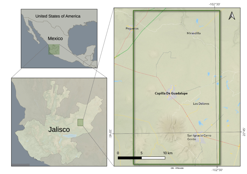
Figure 1: Regional area under study: Capilla de Guadalupe and San Ignacio Cerro Gordo municipalities of Jalisco, Mexico.

We used Worldview-2 RGB-images (2019 and 2020) and their corresponding labels (digitized by expert photointerpreters using QGIS) as training data.

3.1 Agave crop segmentation

Worldview-2 data and their labels were grouped in Grid (G) elements generating the pairs $P_{G}=(R_{G},L_{G})$. Then, a pair mask ($P_{M}=(R_{M},L_{M})$) was generated with an 8-bits re-sampling and a binary raster mask (as segmentation label). After that, a 256x256 cropping was applied to rasters and labels, defined by pair crop $P_{C}=(R_{C},L_{C})$. The cropping is due to the GPU memory size limitation (16 GB). In Figure 2 it is possible to see a graphic description of these pre-processing steps.

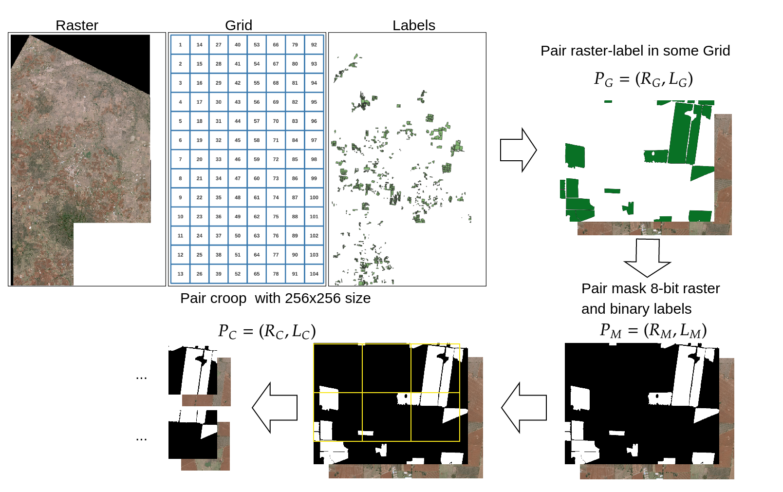
Figure 2: Agave crop segmentation Pre-processing steps.

The number of initial 256$\times$256 pixel data-element clips (RGB images) with their matching binary mask are presented in Table 2.

Split data	Number of elements	Grid ID
Training	127	32, 48 and 71
Validation	48	32, 48 and 71
Testing	208	7, 9, 34, 45, 47, 57, 58 and 60
Total	383

Table 2: Number of 256 $\times$ 256 images clips and labels in the initial phase for training, validation, and testing.

In Figure 3, we present an example of the original data (phase 1 data) and matching labels. It is important to note that those polygons (labels) include not only the agave crops but may also include trees, water, houses, bushes, etc. The noisy label is one of the main characteristics of real-world problems (often called in the wild [8]).

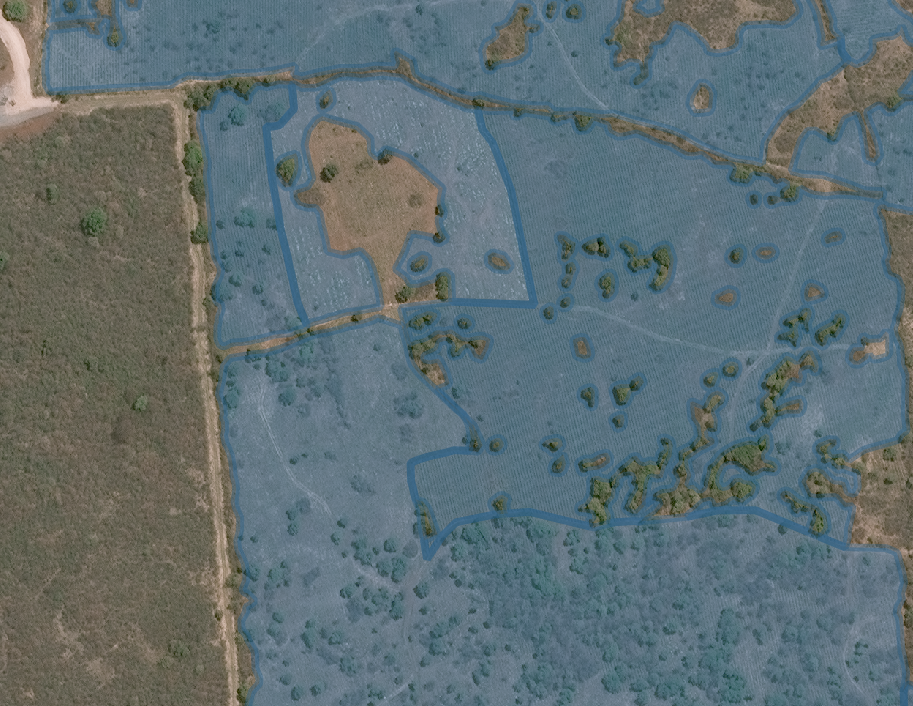
Figure 3: Example of initial phase agave crop segmentation labels. Note that some trees, walking paths, and bushes are wrongly included in the agave crops labels.

3.2 Agave maturity classification

To obtain agave maturity data, we split every tile into $32\times 32$ pixels. We defined two classes: young agave (less than or equal to two years of age) and mature agave (more than two years of age). Agave maturity classification labels were prepared by expert photo-interpreters using QGIS and images from different dates were compared to validate evolution of the agave’s maturity. Figure 4 illustrates the process for extracting the agave maturity tiles (32$\times$32 pixels) and labels $(B_{A},L_{A}),$ respectively. Note that we selected only those full tiles (yellow bounding-boxes) which are inside the plot limits and that the partial tiles denoted by dashed red lines are not candidates for maturity classification. In this image, light green represents young agave (less than or equal to 2 years) and dark green r mature agave.

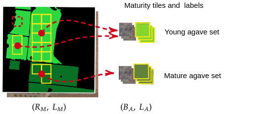
Figure 4: Agave maturity tile extraction. Light green means young agave (up to 2 years) and dark green is mature agave. Yellow bounding-boxes (tiles) represent the locations where a tile was available for extraction, while red bounding-boxes denote unfit tiles.

Table 3 presents the number of (32$\times$32 pixel) samples for training, validation, and testing. Note that both classes are balanced.

Maturity set	Mature	Young	Total
Training	3,904	3,904	7,808
Validation	1,735	1,735	3,470
Testing	1,301	1,301	2,602
Total			13,880

Table 3: Number of 32$\times$32 tiles generated for the agave maturity classification training process.

4 Methods

In this section, we describe the methods, metrics and tools used to achieve agave crop segmentation and maturity classification. The main method for improving results was inspired by the AI-Life cycle [24] in combination with the active learning process and synthetic satellite image generation.

4.1 Agave crop segmentation

Some recurrent challenges of deep learning-real world applications are small training datasets and low-quality labels. As a result, we decided to apply several techniques which could be grouped into three main phases. Figure 5 illustrates some examples of images and labels in each phase. In Phase 1, we show a sample of the original labels, where trees, bushes, and footpaths result in additional label noise. In Phase 2, it can be seen that the improved labels omit trees, bushes, road, footpaths, etc. after using the active learning cycle (human experts+models). The Phase 3 image shows an example of fake/synthetic agave crops. In the following subsections we explain in more detail each phase of crop segmentation.

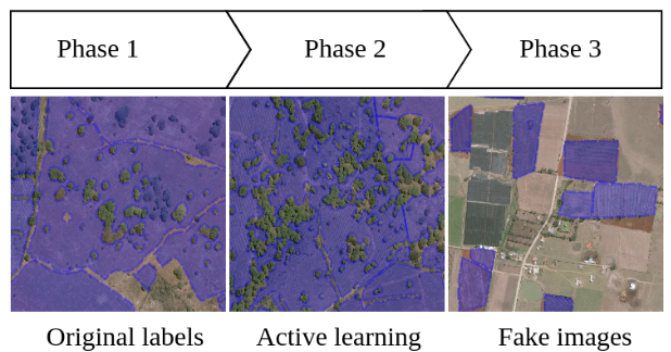
Figure 5: In each phase we present an image to illustrate the original labels (phase 1), improved labels (phase 2), and fake/synthetic images (phase 3).

4.1.1 Phase 1: Training, evaluation and testing using original labels

As noted above, we trained with two well-known regularization techniques: i) transfer learning, i.e the backbone model has been pre-trained with the COCO dataset, and ii) data augmentation. After that, we evaluated the model’s performance in the test set using DCL and IoU. These results are considered the performance baseline for comparison with our models and data.

4.1.2 Phase 2: Active learning

In the second phase, we focused on active learning. Specifically, experts improved agave crop delimitation avoiding inside the crops roads, trees, bushes, houses, water, etc. This technique also helped to increase the number of training samples/labels with a DL-model $+$ human workflow. To do this, the inferences from the DL model propose new labeled areas and human-experts correct and approve the new samples with the corresponding labels.

4.1.3 Phase 3: Synthetic/fake images

In phase 3, we generated synthetic images based on the model’s most frequent validation error (out-of-distribution-data) using an GNU Image Manipulation Program GIMP. Two examples of the phase 1-2 errors are presented in the Figure 6. These examples help to define the textures and regions in the synthetic images.

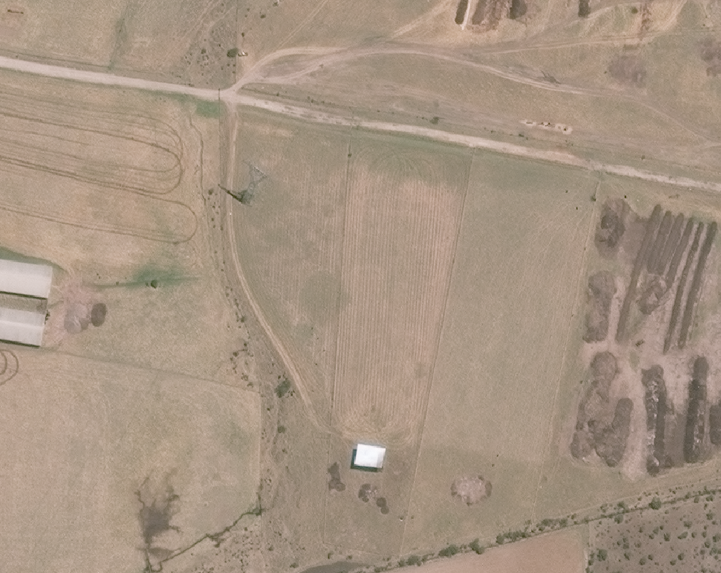
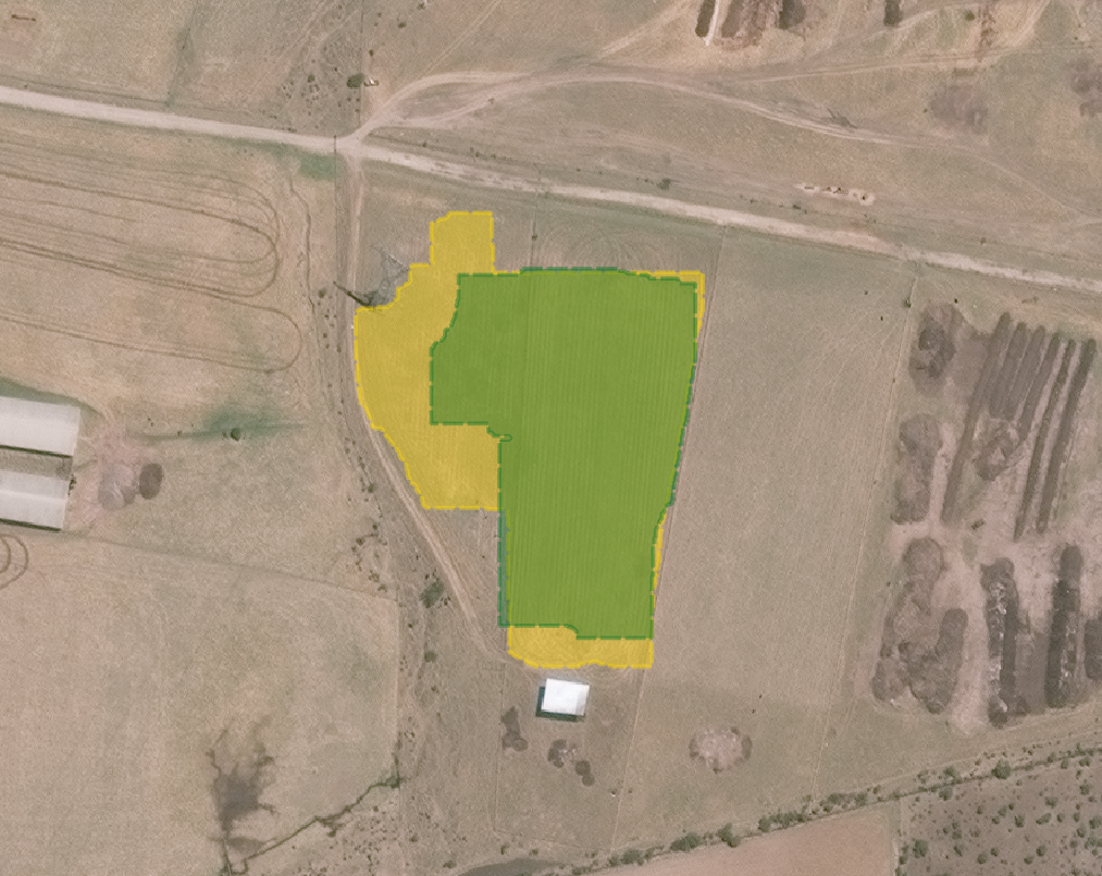
Figure 6: Left: Original image. Center model’s inference and label. Right examples of synthetic/fake images.

4.1.4 Segmentation metrics

The metrics selected to evaluate agave crop segmentation performance models are: Dice Coefficient Loss (DCL) and Intersection Over Union (IoU). The main reason for using these metrics is due to those metrics being widely used in many semantic segmentation tasks [25, 26, 27]. Moreover, IoU is frequently employed as the cutoff point for deciding whether objects should be classified as True Positives (TP) or False Negatives (FN), with 0.5 as the threshold. In addition, DCL and IoU allow the evaluation of highly unbalance classes [26, 28].

DCL is implemented using the Segmentation Models Library. In this library, DCL is computed based on the Dice Similarity Index ($DSI$) defined by equation 1 as follows:

$$DSI=\frac{2|X\cap Y|}{|X|+|Y|}.$$ (1)

For Jaccard index or $IoU$ we also used the implementation from Segmentation Models Library which is fully compatible with our Pytorch implementation. $IoU$ Equation 2 is defined as follows:

$$IoU={{|X\cap Y|}\over{|X\cup Y|}}={{|X\cap Y|}\over{|X|+|Y|-|X\cap Y|}}.$$ (2)

In equations 1 and 2 the two sets $X,Y\in[0,1]$ represent the ground truth label and the model inference value respectively. In addition, $X\cap Y$ represent the pixel-to-pixel intersection, $X\cup Y$ is the union of the two sets, and $|X|$, $|Y|$ is the cardinality of the two sets $X$, $Y$, respectively, i.e, the number of pixels in each set [29].

4.1.5 ConvNets models

The ConvNets used in this work for crop segmentation are Mask R-CNN [12], Unet++ [13], DeepLabV3+ [14] y FPN [15]. In all phases we used transfer learning using COCO [30] weights, and the same data augmentation: $90^{o}$ random rotations, horizontal and, vertical splits in the training set. The hyper-parameters of the training process are a learning rate of 0.0001, and 50 epochs. We used an IBM AC-922 server with four V100 GPU (16GB) for all training.

4.2 Agave maturity classification model

Agave maturity tile classification was carried out using pretrained MobileNetV2 [16], ResNet18 [17] and EfficientNet B0 [18], with a learning rate of 0.0001, an Adam [31] optimizer, and categorical cross entropy loss. In addition, we used data augmentation techniques such as horizontal and vertical flips and random rotations up to $90^{o}$. For all training, we used an IBM AC-922 server with V100 GPU (16GB). To evaluate the model’s performance, we used the following:

$$accuracy = \frac{TP+TN}{TP+TN+FP+FN},$$ (3)

$$sensitivity = \frac{TP}{TP+FN},$$ (4)

$$specificity = \frac{TP}{TN+FP},$$ (5)

where $TP=$ True Positive, $TN=$ True Negative, $FP=$ False Negative, and $FP=$ False Positive.

Figure 7 introduces the process for evaluating the maturity of agave parcels. Each parcel tile (yellow box) is classified using the pretrained ConvNet and then computing the mode to assign the maturity of the parcel.

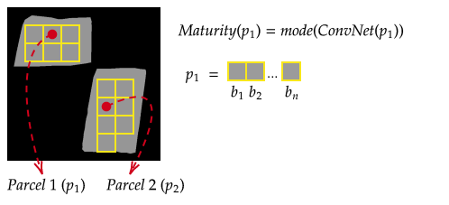
Figure 7: Example of the agave maturity classification computation process. First, we appied the inference using the ConvNet model in each parcel tile, and then we computed the mode.

5 Results and analysis

5.1 Agave crop segmentation

Table 4 presents the number of elements in train-set, validation-set and test-set in each phase. It is important to highlight that the number of training and validation samples increase in each phase. Moreover, our experience hasdemostrated empirically that human/model collaboration reduces the labeling time of human experts. Informally, we note that the labeling time was reduced by a range of factor between 3 to 5.

Figure 8 shows five test-set examples using the phase 3 data. The first column presents the Original RGB image and the second is ground truth label. The following columns present the segmentation results from the Mask R-CNN, Unet++, DeepLabV3+, and FPN, respectively. It can be seen that all models could detect the agave crops in sample images. However, due to post-processing age estimation, we consider better the crop split capacity of the Mask R-CNN.

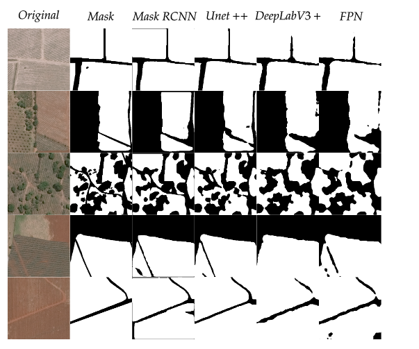
Figure 8: Original RGB images, ground truth labels, and segmentation results from different models: Mask R-CNN, Unet++, DeepLabV3+ and FPN.

Segmentation Set	Phase 1	Phase 2	Phase 3
Training	127	182	528
Validation	48	74	222
Testing	208	208	208
Total	383	464	958

Table 4: Number of ($256\times 256$) clips in training-set, validation-set and test-set in each phase.

Table 5 presents each model’s agave crop segmentation performance numerically. The mean $IoU$ values increase from initial phase from 0.725 to 0.905 in the final phase (higher values is better) and $DCL$ mean value from the initial phase 0.175 to 0.047 in the final phase (lower values are better). Note that the significantly increase in the segmentation performance is from phase 2 to phase 3 where synthetic images and the active learning process are included only in the training set. Comparing the four ConvNet models the MaskRCNN models achieves the best segmentation performance against other ConvNets models. As a result, we consider the Mask R-CNN to have the best qualitative and quantitative results.

Architecture	Phase 1		Phase 2		Phase 3		Param(M)
	$IoU$	$DCL$	$IoU$	$DCL$	$IoU$	$DCL$
Mask RCNN [12]	0.76	0.15	0.74	0.18	0.91	0.047	49.9
Unet++ [13]	0.74	0.18	0.76	0.17	0.91	0.05	48.5
DeepLabV3+ [14]	0.70	0.19	0.72	0.18	0.90	0.05	26.1
FPN [15]	0.70	0.18	0.71	0.17	0.90	0.054	25.6
Mean	0.725	0.175	0.733	0.175	0.905	0.050	–

Table 5: Comparison between the four models and the three data/label improvement phases.

The most important observation from Tables 5, and 4 is that the active learning and synthetic images not only increase the number of trainable images through an effective human-model collaboration but also increase the data-label quality and models performance.

5.2 Agave maturity classification

The quantitative results of agave maturity classification performance in the test set are presented in Table 6. In our opinion the best trade-off between performance and number of trainable parameters is MobileNetV2. An example of the qualitative results is presented in Figure 9, with the original image and the classification areas in light green (young) and dark green (mature). We wish to underscore that this model helped us realize that the segmentation model made more mistakes in the parcels of young agave due to the similarities between cultivation line patterns and soil color.

Model	Accuracy	Sensitivity	Specificity	Loss	Params (M)
MobileNetV2 [16]	0.97	0.98	0.96	0.079	2.2
Resnet18 [17]	0.97	0.97	0.97	0.084	11.2
EfficientnetB0 [18]	0.97	0.99	0.95	0.101	4

Table 6: Agave maturity classification report on three ConvNet architectures.

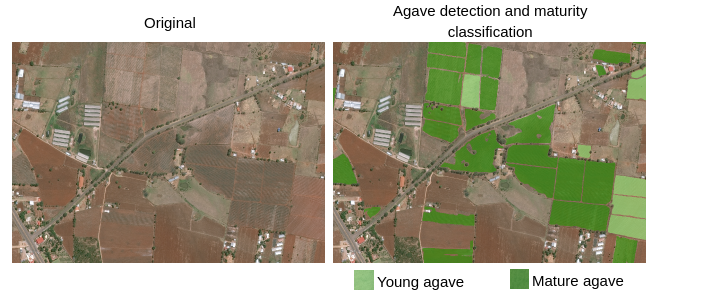
Figure 9: Agave detection and maturity classification example.

6 Conclusions

Our work is the first to implement deep learning techniques for these agave tasks on this scale. Moreover, this work presents a novel strategy for large-scale DL agave-parcel segmentation and maturity classification using very high-resolution satellite imagery. The proposed strategy solves typical DL real-word problems such as a lack of data, low-quality labels, poor model performance and highly imbalanced data in the very specific context of agave. This strategy combines active learning, and data-centric (synthetic image/label generation) techniques. According to the results, this strategy allows significantly increase the number of samples/labels and segmentation performance in less time and with effort on the part of photointerpreters. This could have a major impact on monitoring and mapping tasks, reducing the time required to digitize agave crops compared to traditional human only methods. Regarding the DL models, Mask-R CNN had the best trade-off between IoU, DL and the number of trainable parameters. This agave maturity classification method is 95 %, accurate; however, we detected more error (biases) in the young agave class. These models can be used to monitor large regions, on the order of thousands of squared kilometers, and can contribute to reducing social and environmental problems resulting from the agave-tequila production chain. As a future work, we are planning to use other satellite imagery to detect agave crops.

Acknowledgments. The authors would like to thank CONACYT, and SEMADET for their valuable help.

Data availability. The data that support the findings of this study are available from Maxar but restrictions apply to the availability of these data, which were used under license for the current study, and so are not publicly available. Data are however available from the authors upon reasonable request and with permission of Maxar. The corresponding labels, models and code are available from the corresponding author upon reasonable request.

Declarations

Conflict of interest. The authors declare that they have no conflict of interest.

References

- [1] J. Gallardo, “Industria del tequila y generación de residuos,” Ciencia y Desarrollo CONACYT. http://www. cienciaydesarrollo. mx, 2018.
- [2] Consejo Regulador del Tequila, A.C, Consejo Regulador del Tequila (CRT), 2022.
- [3] “Tequila libre de deforestación; acciones ante el cambio climático,” 2022.
- [4] B. T. Kitano, C. C. Mendes, A. R. Geus, H. C. Oliveira, and J. R. Souza, “Corn plant counting using deep learning and uav images,” IEEE Geoscience and Remote Sensing Letters, 2019.
- [5] D. Flores, I. González-Hernández, R. Lozano, J. M. Vazquez-Nicolas, and J. L. Hernandez Toral, “Automated agave detection and counting using a convolutional neural network and unmanned aerial systems,” Drones, vol. 5, no. 1, 2021.
- [6] A. Quevedo, A. Sánchez, R. Nancláres, D. P. Montoya, J. Pacho, J. Martínez, and E. U. Moya-Sánchez, “Jalisco’s multiclass land cover analysis and classification using a novel lightweight convnet with real-world multispectral and relief data,” 2022.
- [7] I. Bhakta, S. Phadikar, K. Majumder, H. Mukherjee, and A. Sau, “A novel plant disease prediction model based on thermal images using modified deep convolutional neural network,” Precision Agriculture, pp. 1–17, 2022.
- [8] T. Stadelmann, M. Amirian, I. Arabaci, M. Arnold, G. F. Duivesteijn, I. Elezi, M. Geiger, S. Lörwald, B. B. Meier, K. Rombach, et al., “Deep learning in the wild,” in IAPR Workshop on Artificial Neural Networks in Pattern Recognition, pp. 17–38, Springer, 2018.
- [9] S. Dodge and L. Karam, “Understanding how image quality affects deep neural networks,” in 2016 eighth international conference on quality of multimedia experience (QoMEX), pp. 1–6, IEEE, 2016.
- [10] E. U. Moya-Sánchez, S. Xambó-Descamps, A. S. Pérez, S. Salazar-Colores, and U. Cortés, “A trainable monogenic convnet layer robust in front of large contrast changes in image classification,” IEEE access, vol. 9, pp. 163735–163746, 2021.
- [11] S. E. Whang, Y. Roh, H. Song, and J.-G. Lee, “Data collection and quality challenges in deep learning: A data-centric ai perspective,” The VLDB Journal, pp. 1–23, 2023.
- [12] K. He, G. Gkioxari, P. Dollár, and R. B. Girshick, “Mask R-CNN,” CoRR, vol. abs/1703.06870, 2017.
- [13] Z. Zhou, M. M. R. Siddiquee, N. Tajbakhsh, and J. Liang, “Unet++: A nested u-net architecture for medical image segmentation,” CoRR, vol. abs/1807.10165, 2018.
- [14] L. Chen, Y. Zhu, G. Papandreou, F. Schroff, and H. Adam, “Encoder-decoder with atrous separable convolution for semantic image segmentation,” CoRR, vol. abs/1802.02611, 2018.
- [15] T. Lin, P. Dollár, R. B. Girshick, K. He, B. Hariharan, and S. J. Belongie, “Feature pyramid networks for object detection,” CoRR, vol. abs/1612.03144, 2016.
- [16] M. Sandler, A. G. Howard, M. Zhu, A. Zhmoginov, and L. Chen, “Inverted residuals and linear bottlenecks: Mobile networks for classification, detection and segmentation,” CoRR, vol. abs/1801.04381, 2018.
- [17] K. He, X. Zhang, S. Ren, and J. Sun, “Deep residual learning for image recognition,” CoRR, vol. abs/1512.03385, 2015.
- [18] M. Tan and Q. V. Le, “Efficientnet: Rethinking model scaling for convolutional neural networks,” CoRR, vol. abs/1905.11946, 2019.
- [19] J. G. Escobar-Flores, S. Sandoval, and E. Gámiz-Romero, “Unmanned aerial vehicle images in the machine learning for agave detection,” Environmental Science and Pollution Research, pp. 1–12, 2022.
- [20] G. Calvario, T. E. Alarcón, O. Dalmau, B. Sierra, and C. Hernandez, “An agave counting methodology based on mathematical morphology and images acquired through unmanned aerial vehicles,” Sensors, vol. 20, no. 21, p. 6247, 2020.
- [21] G. Calvario, B. Sierra, T. E. Alarcón, C. Hernandez, and O. Dalmau, “A multi-disciplinary approach to remote sensing through low-cost uavs,” Sensors, vol. 17, no. 6, p. 1411, 2017.
- [22] J. Garnica, R. Reich, E. T. Zuñiga, and C. A. Bravo, “Using remote sensing to support different approaches to identify agave (agave tequilana weber) crops,” Int. Arch. Photogramm. Remote Sens. Spat. Inf. Sci, vol. 37, pp. 941–944, 2008.
- [23] J. Li, J. Tao, L. Ding, H. Gao, Z. Deng, Y. Luo, and Z. Li, “A new iterative synthetic data generation method for cnn based stroke gesture recognition,” Multimedia Tools and Applications, vol. 77, pp. 17181–17205, Jul 2018.
- [24] D. De Silva and D. Alahakoon, “An artificial intelligence life cycle: From conception to production,” Patterns, vol. 3, no. 6, p. 100489, 2022.
- [25] W. Zhang, A. K. Liljedahl, M. Kanevskiy, H. E. Epstein, B. M. Jones, M. T. Jorgenson, and K. Kent, “Transferability of the deep learning mask r-cnn model for automated mapping of ice-wedge polygons in high-resolution satellite and uav images,” Remote Sensing, vol. 12, no. 7, p. 1085, 2020.
- [26] R. Zhao, B. Qian, X. Zhang, Y. Li, R. Wei, Y. Liu, and Y. Pan, “Rethinking dice loss for medical image segmentation,” in 2020 IEEE International Conference on Data Mining (ICDM), pp. 851–860, 2020.
- [27] A. E. Maxwell, T. A. Warner, and L. A. Guillén, “Accuracy assessment in convolutional neural network-based deep learning remote sensing studies—part 1: Literature review,” Remote Sensing, vol. 13, no. 13, p. 2450, 2021.
- [28] L. Zhu, Z. Xie, L. Liu, B. Tao, and W. Tao, “Iou-uniform r-cnn: Breaking through the limitations of rpn,” Pattern Recognition, vol. 112, p. 107816, 2021.
- [29] A. Zijdenbos, B. Dawant, R. Margolin, and A. Palmer, “Morphometric analysis of white matter lesions in mr images: method and validation,” IEEE Transactions on Medical Imaging, vol. 13, no. 4, pp. 716–724, 1994.
- [30] T.-Y. Lin, M. Maire, S. Belongie, J. Hays, P. Perona, D. Ramanan, P. Dollár, and C. L. Zitnick, “Microsoft coco: Common objects in context,” in Computer Vision – ECCV 2014 (D. Fleet, T. Pajdla, B. Schiele, and T. Tuytelaars, eds.), (Cham), pp. 740–755, Springer International Publishing, 2014.
- [31] D. P. Kingma and J. Ba, “Adam: A method for stochastic optimization,” CoRR, vol. abs/1412.6980, 2015.