MODEFORMER: Modality-Preserving Embedding for Audio-Video Synchronization using Transformers

Abstract

Lack of audio-video synchronization is a common problem during television broadcasts and video conferencing, leading to an unsatisfactory viewing experience. A widely accepted paradigm is to create an error detection mechanism that identifies the cases when audio is leading or lagging. We propose ModEFormer, which independently extracts audio and video embeddings using modality-specific transformers. Different from the other transformer-based approaches, ModEFormer preserves the modality of the input streams which allows us to use a larger batch size with more negative audio samples for contrastive learning. Further, we propose a trade-off between the number of negative samples and number of unique samples in a batch to significantly exceed the performance of previous methods. Experimental results show that ModEFormer achieves state-of-the-art performance, 94.5% for LRS2 and 90.9% for LRS3. Finally, we demonstrate how ModEFormer can be used for offset detection for test clips.

Index Terms—  Contrastive learning, audio-video synchronization, transformers, negative sampling

1 Introduction and Related Work

Out-of-sync between audio and video is a critical problem that degrades user experience. This problem occurs quite often due to stochastic uncertainty from physical recording equipment or various network issues. This is more obvious in talking face videos where the lip motion does not align with the progression of audio. Having a lip-audio sync detector is of vital importance to measure and correct offsets between the audio and video streams.

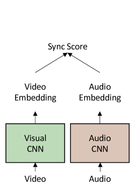
(a) SyncNet / PM

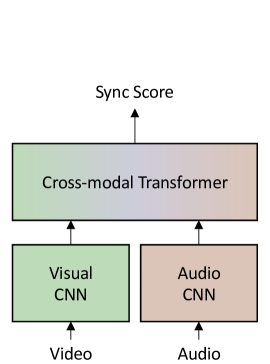
(b) AVST / VocaLiST

(c) ModEFormer - Ours

Fig. 1: Comparison of different architectures for audio-video sync detection. SyncNet [1] and PM [2] encode audio and video inputs independently and compute a sync score by measuring cosine similarity between them. AVST [3] and VocaLiST [4] adopt transformers to predict a sync score directly. They combine audio and visual features inside the cross-modal transformers. Our model has a modality-preserving architecture with transformers, which encodes visual and audio signals independently. By keeping the modality, we enable effective contrastive learning with either a large batch size or more negative examples.

Although traditional methods like time warping have proven to be quite useful in detecting this error, these are human-dependent and seem intractable with the amount of digital media in today’s world. Some of the earliest works include Hershey et al. [5], which calculates the mutual information or “synchrony” and FaceSync [6], which uses the Pearson’s coefficient for audio-video correlation. Other works like Morishima et al. [7] and Lewis et al. [8] use phoneme-viseme matching to ensure audio-video sync.

With the advancement of artificial intelligence, various sync detection techniques have been developed. SyncNet [1] is the first to use convolutional neural networks to extract audio and video embeddings and train them with a contrastive learning objective. Another following work that builds further on this is Perfect Match (PM) [2], which introduces the idea of multi-way matching of an audio embedding with multiple video embeddings by using a multi-way cross-entropy loss. They propose that this multi-way matching is beneficial during contrastive learning since it takes into account contextual information in an input sequence during training. Further, Prajwal et al. [9] presents a slightly different version of SyncNet by using residual convolution neural network (CNN) encoders and a cosine similarity-based loss but limits it to the binary matching of embeddings.

Transformers [10] have emerged as one of the leading models for feature encoding. In audio-video synchronization, transformers have shown significant improvement over CNN-based architectures. Chen et al. [3] introduced AVST or Audio-Video Sync Transformer that provides a generalized solution for synchronization over various sound classes found in in-the-wild videos. They propose a sync transformer module that helps in learning cross-modal relations between the two modalities. Another recent work, VocaLiST [4] offers an improvement over AVST by using multiple such sync transformers learning audio-to-video, video-to-audio, and hybrid correlations. Although the above modifications show improvement in audio-video synchronization, they do not explore sampling strategies for contrastive learning.

In this work, we propose ModEFormer, which is a transformer-based model that extracts audio and video embeddings. We train our model to yield embeddings with high cosine similarities only when the input audio and video are in-sync. Unlike previous transformer-based algorithms [3, 4] that blend modalities inside their models, our method keeps separate audio and visual modalities, and thus enables contrastive learning with a large number of negative examples. Fig. 1 visually compares our ModEFormer’s architecture to the existing methods [3, 4, 1, 2]. We conduct experiments to discover the most beneficial method of composing negative examples for contrastive learning of audio-video sync detection. We demonstrate that our method reaches state-of-the-art performance on both LRS2 [11] and LRS3 [12] datasets. The key contributions of this work are

• Building modality-preserving transformer encoders that enable contrastive learning with larger number of negative examples.

• Propose best trade-off between the number of negative examples and number of unique samples in a batch for optimal training of audio-video out-sync detection.

• Remarkable performance on LRS2 and LRS3 datasets

2 Methodology

We train our model, ModEFormer, to predict a sync score between a facial video and an audio clip. Our model accepts five consecutive frames ($T_{\textrm{v}}=5$) of a lip region as the video input $\mathbf{v}$. We define the lip region as a lower-half of a facial video at $48\times 96$ resolution ($H=48$ and $W=96$) by following the conventional work [4]. We convert a given audio, whose length is corresponding to the five video frames, into a melspectrogram with 80 mel frequencies ($M=80$). We then sample $3.2$ audio frames for each video frame, and thus the input audio $\mathbf{m}$’s shape is $M\times T_{\textrm{a}}$, where $T_{\textrm{a}}=3.2\times T_{\textrm{v}}=16$. We train our model to predict a sync score between these video and audio inputs.

2.1 Architecture of ModEFormer

We visualize the architecture of ModEFormer in Fig. 2. ModEFormer consists of CNN encoders $E$ and transformer encoders $P$ for both audio and video modalities. We design our model using modality-specific transformers and show in Sec 3.1 that they outperform previous transformer and CNN-based sync detectors [4, 3, 1, 2] due to their enhanced ability of negative sampling and contrastive learning. While the CNN encoders extract lower-level representations, we obtain condensed modality-specific embeddings from the transformer encoders for the audio and video inputs.

Lower-level representation using CNN encoders.

For the audio CNN encoder $E_{\mathrm{a}}$, we use an architecture similar to ResNet18 [14]. We replace the first convolution layer to input a 1-channel tensor. We also adjust strides of convolutions to encode an audio input $\mathbf{m}\in\mathbb{R}^{M\times T_{\mathrm{a}}}$ to $E_{\mathrm{a}}(\mathbf{m})\in\mathbb{R}^{512\times T_{\mathrm{a}}}$ features. For the video branch, we obtain a lower-level representation $E_{\mathrm{v}}(\mathbf{f})\in\mathbb{R}^{512\times T_{\mathrm{v}}}$ by passing a video $\mathbf{f}$ through a 3D-CNN encoder $E_{\mathrm{v}}$ to make it learn the temporal information between frames. We adopt an architecture analogous to the audio encoder but with 3D convolutions.

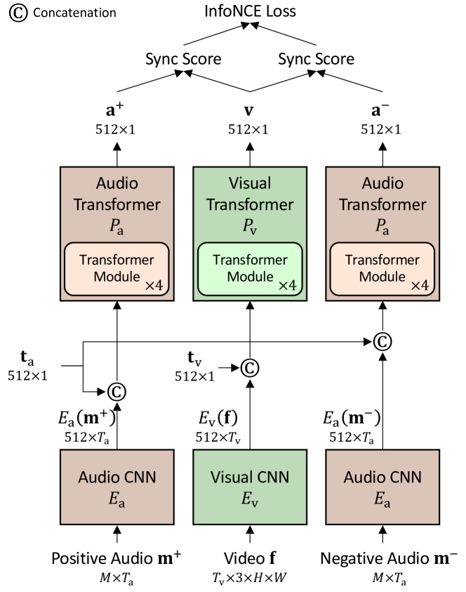
Fig. 2: Architecture of ModEFormer. It takes audio and video inputs ($\mathbf{m}^{-}$, $\mathbf{m}^{+}$, $\mathbf{f}$) and yields respective embeddings ($\mathbf{a}^{-}$, $\mathbf{a}^{+}$, $\mathbf{v}$). We independently encodes the input audio and video by feeding them through the CNN and modality-specific transformer encoders ($E$ and $P$). We employ contrastive learning by minimizing an InfoNCE loss between sync scores of the embeddings.

Table 1: Comparison of audio-video sync detectors on the LRS2 and LRS3 test sets. We measure the synchronization accuracies at different clip lengths. “Var” indicates whether a model has seen clips with variable lengths during training. We only compare the sync detectors trained with a fixed number of input frames. We highlight the best scores in boldface.

			Clip Length in Frames (Seconds)						# of params
Dataset	Model	Var	5 (0.2s)	7 (0.28s)	9 (0.36s)	11 (0.44s)	13 (0.52s)	15 (0.6s)	(M=Millions)
	AVST[3]	✓	91.9	97.0	98.8	99.6	99.8	99.9	42.4M
	SyncNet[1]		75.8	82.3	87.6	91.8	94.5	96.1	13.6M
LRS2	PM[2]		88.1	93.8	96.4	97.9	98.7	99.1	13.6M
	VocaLiST[4]		92.8	96.7	98.4	99.3	99.6	99.8	80.1M
	ModEFormer - Ours		94.5	97.1	98.5	99.3	99.7	99.8	59.0M
LRS3	AVST[3]	✓	77.3	88.0	93.3	96.4	97.8	98.6	42.4M
	ModEFormer - Ours		90.9	93.1	96.0	97.7	98.7	99.2	59.0M

Modality-preserving encoding via transformers.

The existing transformer-based sync detectors [3, 4] blend audio and visual features by exploiting cross-modal attentions to compute a sync score. However, combining modalities within a model makes contrastive learning difficult since a visual input should go through transformers as many times as the number of audio examples. As it requires more GPU memory, a large batch size, which is necessary for contrastive learning, is not usable. We adopt contrastive learning, which is known as effective for representing an embedding space and improving model’s robustness. To this end, we preserve audio and visual modalities and compute a sync score using features from each modality unlike the previous methods.

For an audio feature extracted from the audio CNN, we first concatenate it with an audio class token $\mathbf{t}_{\mathrm{a}}$, and then inject sinusoidal positional encodings [10]. We apply the audio transformer $P_{\mathrm{a}}$, which consists of four transformer modules, to the audio feature. Each transformer encoder is a lighter version of the ViT-Base architecture [15] with 4 layers. We use audio class token’s output from the transformer as ModEFormer’s final audio embedding $\mathbf{a}$. We process a video in the same way using the visual transformer $P_{\mathrm{v}}$ to obtain a final visual embedding $\mathbf{v}$.

2.2 Negative Sampling for Contrastive Learning

We sample two types of negative audio examples - 1) hard negatives which are from the same video clip as the positive audio but temporally shifted. These constitute relatively similar speech features but partially or completely different phrasings. 2) Easy negatives which are from different video clips constituting different phrasings and speaker identities. We define the number of hard negatives used as $N_{\mathrm{H}}$. For a given batch size of $B$, each video has one positive audio and $N_{\mathrm{H}}$ hard negative examples. We train our model in two stages. In the first stage, we use $N_{\mathrm{H}}=2$ hard negatives for each batch entry. We do not use any easy negatives in this stage. Then in the second stage of our training for each batch entry, we use positive audios and their hard negatives in the other batch entries as easy negatives. The number of easy negatives in the second stage becomes $N_{\mathrm{E}}=(B-1)\times(1+N_{\mathrm{H}})$. Due to the GPU memory limit, there is a trade-off between batch size $B$ and number of hard negatives $N_{\mathrm{H}}$, i.e. only small number of hard negatives are usable when a batch size is large. We study this trade-off in our experimental results to find the best ratio for contrastive learning of audio-video sync detection.

Loss function. We first define a similarity $\phi$ between video embedding $\mathbf{v}$ and audio embedding $\mathbf{a}$ as the dot product between their unit vectors.

$$\phi(\mathbf{v},\mathbf{a})=\dfrac{\mathbf{v}}{|\mathbf{v}|}.\dfrac{\mathbf{a}}{|\mathbf{a}|}.$$ (1)

We minimize the InfoNCE loss formulated as

$$L=-\frac{1}{B}\sum_{\mathbf{v},\mathbf{a}^{+}\in\mathcal{P}}\log{\frac{e^{(\phi(\mathbf{v},\mathbf{a}^{+})/\tau)}}{\sum_{\mathbf{a}\in\mathcal{N}(\mathbf{v})}e^{(\phi(\mathbf{v},\mathbf{a})/\tau)}}},$$ (2)

where $\mathcal{P}$ represents a set of video and positive audio pairs and $\mathcal{N}(\mathbf{v})$ indicates a superset of positive, hard negative, and easy negative audios of video $\mathbf{v}$. $\tau$ is a temperature set as $0.1$. The InfoNCE loss maximizes the similarity of a video embedding with a positive audio embedding and simultaneously minimizes it with multiple negative audio embeddings.

3 Experimental Results

We evaluate our method on benchmark datasets, conduct study of the negative sampling for contrastive learning, and showcase our method’s application as an offset detector.

3.1 Experimental Setup

We train ModEFormer using the Adam optimizer with a learning rate of 0.0001. ModEFormer is trained in 2 stages. In the first stage, we train the ModEFormer with a batch size of $2000$ where each batch entry is from a unique clip and has two corresponding hard negative audio samples.

In the second stage, multiple entries in the same batch are drawn from the same clip and report ablation results in Sec 3.3 and Sec 3.4

Datasets. We use two public benchmark datasets for audio-video sync detection, LRS2 [11] and LRS3 [12]. Both LRS2 and LRS3 have English speakers only. LRS2 provides videos cropped around speaker’s face and their corresponding audios. LRS2 consists of 96,318 pretrain, 45,839 train, 1,082 validation, and 1,243 test videos. We train ModEFormer using the pretrain split and use the validation and test video sets for validation and evaluation, respectively. LRS3 consists of audio-video pairs from TED and TEDx. For LRS3, both full-frames and cropped-frames are available, but we use cropped-frames only to be consistent with LRS2. LRS3 includes 1,18,516 pretrain, 31,982 trainval, and 1,321 test videos. We train ModEFormer on the pretrain set and create a validation set by randomly sampling 40% of the trainval partition. Again, their test partition is directly used as the test set. Please note that we follow the standard setting in the previous work [4] to conduct fair comparisons.

Fig. 3: Lip synchronization accuracies on LRS3 for different number of hard negatives. We measure the accuracy at six different clip lengths. The number of hard negatives that maximizes the overall accuracy is depicted in the grey vertical line.

Evaluation metric.

We measure performances of sync detectors by the lip synchronization accuracy, which is a standard metric for benchmarking [4].

For each input clip, we slide an audio window within $\pm 15$ range centered on the audio with the zero offset. We determine sync detector’s prediction is correct only when it gives a maximum score within $\pm 1$ range. The final lip synchronization accuracy is computed by the number of correct predictions over the number of tested clips. We report the lip synchronization accuracy for each algorithm at 6 different clip lengths which are 5, 7, 9, 11, 13, and 15. Since our ModEFormer only accepts 5 frames as the input, we slide our model over 5 frame windows when the length of the clip is longer than 5 frames and then average the cosine distance to compute the accuracy as done in the conventional works [4]. Note that longer clip lengths lead to higher accuracy as more context is available.

3.2 Benchmark Results

Table 1 lists performance of ModEFormer against four different sync detectors: SyncNet [1], PM [2], AVST [3], and VocaList [4]. We assess each algorithm using the lip synchronization accuracy at six different clip lengths. We observe that our ModEFormer significantly and consistently outperforms all the existing methods that use a fixed number of input frames. It is even more interesting to see that our ModEFormer performs better than VocaLiST [4] considering their model (80M parameters) is heavier than ours (59M parameters). We believe the reason for such improvement is due to our modality-preserving architecture and our sampling strategy allowing us to use multiple hard negatives in contrastive learning. We do not directly compare AVST with the other sync detectors because it has seen clips of variable lengths as input during training. As can be seen in Table 1, ModEFormer outperforms AVST significantly by 2.6% on 5-frames but AVST performs better when the length of the frames is more than 7 frames with a difference of less than 0.3%. This can be attributed to their model having the information of all frames when it makes predictions, whereas we use the sliding window strategy explained in Sec 3.1.

Table 1 shows synchronization accuracy of our ModEFormer and AVST [3] on the LRS3 dataset. We present ModEFormer’s performance here to demonstrate the generalizability of our approach. Our ModEFormer achieves the SoTA on LRS3, which aligns with the results on LRS2. To the best of our knowledge, there are no existing works that have evaluated sync detectors on LRS3’s cropped faces. AVST’s accuracy is available for LRS3, but unfortunately, they use full-frame videos.

Table 2: Results of 3D-SyncNet and ModEFormer on LRS3 test set

	3D-SyncNet	ModEFormer	ModEFormer
		(1st stage)	(2nd stage)
Accuracy	80.2%	88.3%	90.9%

3.3 Architecture Ablation

Table 2 compares 3D-SyncNet and ModEFormer in both the training stages as described in Sec. 3.1, on the LRS3 test set in terms of the lip synchronization accuracy at the clip length of five frames. We build 3D-SyncNet by ablating transformers from ModEFormer. We train both the models with the same InfoNCE loss and sampling strategy. Ablation of the transformer encoders decreases the performance from 88.3% to 80.2%, which shows that attention helps in learning better latent representations. Further, we also see the benefit of the second stage training with more negative examples for ModEFormer improving by 2.6%.

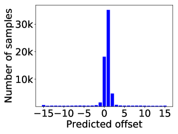
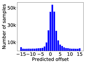
(a)	(b)
Trained on LRS2 and tested on (a) LRS3, (b) VoxCeleb2
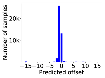
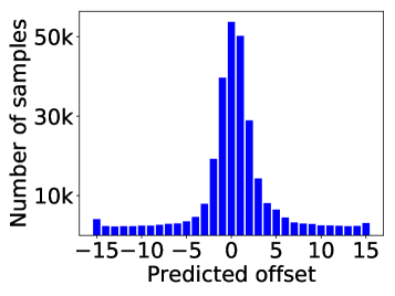
(c)	(d)
Trained on LRS3 and tested on (c) LRS2, (d) VoxCeleb2

Fig. 4: Histogram of predicted offsets for ModEFormer models tested on out of distribution datasets

3.4 Negative Sampling Strategy

We experiment further to find the optimal number of hard negatives between 2 to 25 by measuring the lip synchronization accuracy. Fig. 3 illustrates the accuracies for LRS3 at clip lengths of 5, 7, 9, 11, 13, and 15 frames in accordance with the number of hard negatives. We see that the overall lip sync accuracy peaks when the number of hard negatives is 11. This shows that balancing between the number of hard negatives and batch size is important to maximize performance.

3.5 Offset Detection

We apply a trained ModEFormer to detect any audio-video lag in a given test clip. For a given clip, we compute the cosine similarities at every video frame for audio windows in its neighborhood as described in Sec 3.1. We identify the predicted offset for each video frame as the audio window with the highest cosine similarity. Then we generate the histogram of predicted offsets for each of the video frames in the test clip as shown in Fig. 4. The largest peak of the predicted offset histogram indicates the offset in the test clip. Note that this offset is in comparison to the training dataset used for training the ModEFormer.

Using this mechanism, we discovered that the LRS2 and LRS3 datasets are not in sync with one another. The largest peak of the predicted offset is $+1$ (+0.04s) when using a ModEFormer trained on LRS2 and tested on the LRS3 test set, Fig. 4(a). In parallel, for a ModEFormer trained on LRS3 and tested on LRS2 test set, the offset is at $-1$ (-0.04s), Fig 4(c). To hypothesize which of the datasets is out of sync, we tested models from both LRS2 and LRS3 on an out of distribution test dataset of 1,568 random clips from VoxCeleb2 [16] which is a multi-lingual dataset with noisier audio than LRS2 and LRS3 [17]. We find that an LRS3 trained model has the largest peak of the predicted offset at $0$, Fig. 4(d) while the largest peak of the predicted offset for an LRS2 trained model is $1$, Fig. 4(b). These results lead us to hypothesize that LRS3 and VoxCeleb2 are in sync while LRS2 is out of sync.

Further, if we shift the audio windows in the LRS2 test set with an offset of $+1$, the accuracy of the LRS3 model on the test set increases from 88.27% to 91.39%. In future experiments, we recommend accounting for this offset when reporting performance across the datasets.

4 Conclusion

We present a modality-preserving sync detector, ModEFormer, which yields state-of-the-art performance on both the LRS2 and LRS3 datasets. Since ModEFormer preserves the modality, we are able to trade-off between the number of negative examples and the number of unique samples in a batch to find the most optimal configuration. Further, we demonstrate offset detection using ModEFormer for an out-of-distribution test dataset and hypothesize that LRS2 and LRS3 are out-of-sync by +0.04 seconds

References

- [1] Joon Son Chung and Andrew Zisserman, “Out of time: automated lip sync in the wild,” in Workshop on Multi-view Lip-reading, ACCV, 2016.
- [2] Soo-Whan Chung, Joon Son Chung, and Hong-Goo Kang, “Perfect Match: Improved cross-modal embeddings for audio-visual synchronisation,” in IEEE ICASSP, 2019.
- [3] Honglie Chen, Weidi Xie, Triantafyllos Afouras, Arsha Nagrani, Andrea Vedaldi, and Andrew Zisserman, “Audio-visual synchronization in the wild,” in BMVC, 2021.
- [4] Venkatesh Shenoy Kadandale, Juan F. Montesinos, and Gloria Haro, “VocaLiST: An Audio-Visual Synchronisation Model for Lips and Voices,” in Interspeech, 2022.
- [5] John Hershey and Javier Movellan, “Audio Vision: Using audio-visual synchrony to locate sounds,” in NeurIPS, 1999.
- [6] Malcolm Slaney and Michele Covell, “FaceSync: A linear operator for measuring synchronization of video facial images and audio tracks,” in NeurIPS, 2000.
- [7] Shigeo Morishima, Shin Ogata, Kazumasa Murai, and Satoshi Nakamura, “Audio-visual speech translation with automatic lip syncqronization and face tracking based on 3-d head model,” in IEEE ICASSP, 2002.
- [8] John Lewis, “Automated lip-sync: Background and techniques,” The Journal of Visualization and Computer Animation, vol. 2, no. 4, pp. 118–122, 1991.
- [9] K R Prajwal, Rudrabha Mukhopadhyay, Vinay P. Namboodiri, and C.V. Jawahar, “A lip sync expert is all you need for speech to lip generation in the wild,” in ACM International Conference on Multimedia, 2020.
- [10] Ashish Vaswani, Noam Shazeer, Niki Parmar, Jakob Uszkoreit, Llion Jones, Aidan N Gomez, L ukasz Kaiser, and Illia Polosukhin, “Attention is all you need,” in NeurIPS, 2017.
- [11] Triantafyllos Afouras, Joon Son Chung, Andrew Senior, Oriol Vinyals, and Andrew Zisserman, “Deep audio-visual speech recognition,” IEEE Transactions on Pattern Analysis and Machine Intelligence, 2018.
- [12] Triantafyllos Afouras, Joon Son Chung, and Andrew Zisserman, “Lrs3-ted: a large-scale dataset for visual speech recognition,” arXiv:1809.00496, 2018.
- [13] Stavros Petridis, Themos Stafylakis, Pingehuan Ma, Feipeng Cai, Georgios Tzimiropoulos, and Maja Pantic, “End-to-end audiovisual speech recognition,” in 2018 IEEE International Conference on Acoustics, Speech and Signal Processing (ICASSP), 2018, pp. 6548–6552.
- [14] Kaiming He, Xiangyu Zhang, Shaoqing Ren, and Jian Sun, “Deep residual learning for image recognition,” in IEEE CVPR, 2016.
- [15] Alexey Dosovitskiy, Lucas Beyer, Alexander Kolesnikov, Dirk Weissenborn, Xiaohua Zhai, Thomas Unterthiner, Mostafa Dehghani, Matthias Minderer, Georg Heigold, Sylvain Gelly, et al., “An image is worth 16x16 words: Transformers for image recognition at scale,” in International Conference on Learning Representations, 2020.
- [16] Joon Son Chung., Arsha Nagrani, and A. Zisserman, “Voxceleb2: Deep speaker recognition,” in INTERSPEECH, 2018.
- [17] Triantafyllos Afouras, Joon Son Chung, and Andrew Zisserman, “Asr is all you need: Cross-modal distillation for lip reading,” in IEEE ICASSP, 2020.