Indeterminate Probability Neural Network

Abstract

We propose a new general model called IPNN – Indeterminate Probability Neural Network, which combines neural network and probability theory together. In the classical probability theory, the calculation of probability is based on the occurrence of events, which is hardly used in current neural networks. In this paper, we propose a new general probability theory, which is an extension of classical probability theory, and makes classical probability theory a special case to our theory. Besides, for our proposed neural network framework, the output of neural network is defined as probability events, and based on the statistical analysis of these events, the inference model for classification task is deduced. IPNN shows new property: It can perform unsupervised clustering while doing classification. Besides, IPNN is capable of making very large classification with very small neural network, e.g. model with 100 output nodes can classify 10 billion categories. Theoretical advantages are reflected in experimental results. (Source code: https://github.com/Starfruit007/ipnn)

1 Introduction

Humans can distinguish at least 30,000 basic object categories (Biederman, 1987), classification of all these would have two challenges: It requires huge well-labeled images; Model with softmax for large scaled datasets is computationally expensive. Zero-Shot Learning – ZSL (Lampert et al., 2009; Fu et al., 2018) method provides an idea for solving the first problem, which is an attribute-based classification method. ZSL performs object detection based on a human-specified high-level description of the target object instead of training images, like shape, color or even geographic information. But labelling of attributes still needs great efforts and expert experience. Hierarchical softmax can solve the computationally expensive problem, but the performance degrades as the number of classes increase (Mohammed & Umaashankar, 2018).

Probability theory has not only achieved great successes in the classical area, such as Naïve Bayesian method (Cao, 2010), but also in deep neural networks (VAE (Kingma & Welling, 2014), ZSL, etc.) over the last years. However, both have their shortages: Classical probability can not extract features from samples; For neural networks, the extracted features are usually abstract and cannot be directly used for numerical probability calculation. What if we combine them?

There are already some combinations of neural network and bayesian approach, such as probability distribution recognition (Su & Chou, 2006; Kocadağlı & Aşıkgil, 2014), Bayesian approach are used to improve the accuracy of neural modeling (Morales & Yu, 2021), etc. However, current combinations do not take advantages of ZSL method.

We propose an approach to solve the mentioned problems, and our contributions are summarized as follows:

• We propose a new general probability theory – indeterminate probability theory, which is an extension of classical probability theory, and makes classical probability theory a special case to our theory.

• We interpret the output neurons of neural network as events of discrete random variables, and indeterminate probability is defined to describe the uncertainty of the probability event state.

• We propose a novel unified combination of (indeterminate) probability theory and deep neural network. The neural network is used to extract attributes which are defined as discrete random variables, and the inference model for classification task is derived. Besides, these attributes do not need to be labeled in advance.

The rest of this paper is organized as follows: In Section 2, we first introduce a coin toss game as example of human cognition to explain the core idea of IPNN. In Section 3, the model architecture and indeterminate probability is derived. Section 4 discusses the training strategy and related hyper-parameters. In Section 5, we evaluate IPNN and make an impact analysis on its hyper-parameters. Finally, we put forward some future research ideas and conclude the paper in Section 6.

2 Background

Let’s first introduce a small game – coin toss: a child and an adult are observing the outcomes of each coin toss and record the results independently (heads or tails), the child can’t always record the results correctly and the adult can record it correctly, in addition, the records of the child are also observed by the adult. After several coin tosses, the question now is, suppose the adult is not allowed to watch the next coin toss, what is the probability of his inference outcome of next coin toss via the child’s record?

As shown in Figure 1, random variables X is the random experiment itself, and $X=x_{k}$ represent the $k^{th}$ random experiment. Y and A are defined to represent the adult’s record and the child’s record, respectively. And $hd,tl$ is for heads and tails. For example, after 10 coin tosses, the records are shown in Table 1.

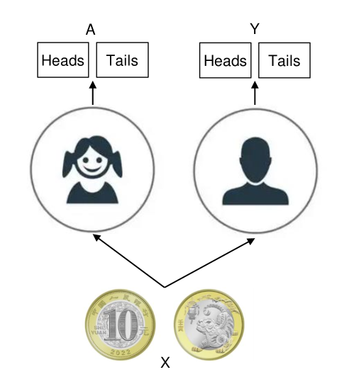
Figure 1: Example of coin toss game.

Table 1: Example of 10 times coin toss outcomes

Experiment	Truth	A	Y
$X=x_{1}$	$hd$	$A=hd$	$Y=hd$
$X=x_{2}$	$hd$	$A=hd$	$Y=hd$
$X=x_{3}$	$hd$	$A=hd$	$Y=hd$
$X=x_{4}$	$hd$	$A=hd$	$Y=hd$
$X=x_{5}$	$hd$	$\mathbf{A=tl}$	$Y=hd$
$X=x_{6}$	$tl$	$A=tl$	$Y=tl$
$X=x_{7}$	$tl$	$A=tl$	$Y=tl$
$X=x_{8}$	$tl$	$A=tl$	$Y=tl$
$X=x_{9}$	$tl$	$A=tl$	$Y=tl$
$X=x_{10}$	$tl$	$A=tl$	$Y=tl$
$X=x_{11}$	$hd$	A=?	Y=?

We formulate X compactly with the ground truth, as shown in Table 2 and Table 3.

Table 2: Outcomes of 10 times coin toss: $P(X)$

$\frac{\#(X)}{n}$	$X=hd$	$X=tl$
	5/10	5/10

Table 3: The adult’s and child’s records: $P(Y|X)$ and $P(A|X)$

$\frac{\#(Y,X)}{\#(X)}$	$Y=hd$	$Y=tl$
$X=hd$	5/5	0
$X=tl$	0	5/5
$\frac{\#(A,X)}{\#(X)}$	$A=hd$	$A=tl$
$X=hd$	4/5	1/5
$X=tl$	0	5/5

Through the adult’s record Y and the child’s records A, we can calculate the conditional probability of Y given A, as shown in Table 4. We define this process as observation phase.

Table 4: Results of observation phase: $P(Y|A)$

$\frac{\#(Y,A)}{\#(A)}$	$Y=hd$	$Y=tl$
$A=hd$	4/4	0
$A=tl$	1/6	5/6

For next coin toss ($X=x_{11}$), the question of this game is formulated as calculation of the probability $P^{A}(Y|X)$, superscript A indicates that Y is inferred via record A, not directly observed by the adult.

For example, given the next coin toss $X=hd=x_{11}$, the child’s record has then two situations: $P(A=hd|X=hd=x_{11})=4/5$ and $P(A=tl|X=hd=x_{11})=1/5$. With the adult’s observation of the child’s records, we have $P(Y=hd|A=hd)=4/4$ and $P(Y=hd|A=tl)=1/6$. Therefore, given next coin toss $X=hd=x_{11}$, $P^{A}(Y=hd|X=hd=x_{11})$ is the summation of these two situations: $\frac{4}{5}\cdot\frac{4}{4}+\frac{1}{5}\cdot\frac{1}{6}$. Table 5 answers the above mentioned question.

Table 5: Results of inference phase: $P^{A}(Y|X)$

$\sum_{A}\left(\frac{\#(A,X)}{\#X}\cdot\frac{\#(Y,A)}{\#A}\right)$	$Y=hd$	$Y=tl$
$X=hd=x_{11}$	$\frac{4}{5}\cdot\frac{4}{4}+\frac{1}{5}\cdot\frac{1}{6}$	$\frac{4}{5}\cdot 0+\frac{1}{5}\cdot\frac{5}{6}$
$X=tl=x_{11}$	$0\cdot\frac{4}{4}+\frac{5}{5}\cdot\frac{1}{6}$	$0\cdot 0+\frac{5}{5}\cdot\frac{5}{6}$

Let’s go one step further, we can find that even the child’s record is written in unknown language (e.g. $A\in\{ZHENG,FAN\}$), Table 4 and Table 5 can still be calculated by the man. The same is true if the child’s record is written from the perspective of attributes, such as color, shape, etc.

Hence, if we substitute the child with a neural network and regard the adult’s record as the sample labels, although the representation of the model outputs is unknown, the labels of input samples can still be inferred from these outputs. This is the core idea of IPNN.

3 IPNN

3.1 Model Architecture

Let $X\in\{x_{1},x_{2},\dots,x_{n}\}$ be training samples ($X=x_{k}$ is understood as $k^{th}$ random experiment – select one train sample.) and $Y\in\{y_{1},y_{2},\dots,y_{m}\}$ consists of $m$ discrete labels (or classes), $P(y_{l}|x_{k})=y_{l}(k)\in\{0,1\}$ describes the label of sample $x_{k}$. For prediction, we calculate the posterior of the label for a given new input sample $x_{n+1}$, it is formulated as $P^{\mathbb{A}}\left(y_{l}\mid x_{n+1}\right)$, superscript $\mathbb{A}$ stands for the medium – model outputs, via which we can infer label $y_{l},\enspace l=1,2,\dots,m$. After $P^{\mathbb{A}}\left(y_{l}\mid x_{n+1}\right)$ is calculated, the $y_{l}$ with maximum posterior is the predicted label.

Figure 2 shows IPNN model architecture, the output neurons of a general neural network (FFN, CNN, Resnet (He et al., 2016), Transformer (Vaswani et al., 2017), Pretrained-Models (Devlin et al., 2019), etc.) is split into N unequal/equal parts, the split shape is marked as Equation 1, hence, the number of output neurons is the summation of the split shape, see Equation 2. Next, each split part is passed to ‘softmax’, so the output neurons can be defined as discrete random variable $A^{j}\in\left\{a_{1}^{j},a_{2}^{j},\dots,a_{M_{j}}^{j}\right\},j=1,2,\dots,N$, and each neuron in $A^{j}$ is regarded as an event. After that, all the random variables together forms the N-dimensional joint sample space, marked as $\mathbb{A}=(A^{1},A^{2},\dots,A^{N})$, and all the joint sample points are fully connected with all labels $Y\in\{y_{1},y_{2},\dots,y_{m}\}$ via conditional probability $P\left(Y=y_{l}|A^{1}=a_{i_{1}}^{1},A^{2}=a_{i_{2}}^{2},\dots,A^{N}=a_{i_{N}}^{N}\right)$, or more compactly written as $P\left(y_{l}|a_{i_{1}}^{1},a_{i_{2}}^{2},\dots,a_{i_{N}}^{N}\right)$.

$$\text{Split shape}:=\{M_{1},M_{2},\dots,M_{N}\}$$ (1)

$$\text{Number of model output neurons}:={\textstyle\sum_{j=1}^{N}M_{j}}$$ (2)

$$\text{Number of joint sample points}:={\textstyle\prod_{j=1}^{N}}M_{j}$$ (3)

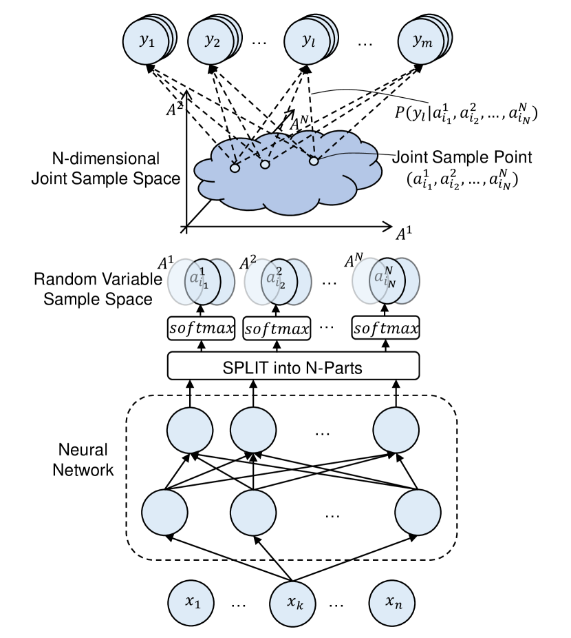
Figure 2: IPNN – model architecture. With the increase of number of random variables, the joint sample points increases exponentially, see Equation 3, but $P\left(y_{l}|a_{i_{1}}^{1},a_{i_{2}}^{2},\dots,a_{i_{N}}^{N}\right)$ is statistically calculated, not model weights.

3.2 Indeterminate Probability Theory

In classical probability theory, given a sample $x_{k}$ (perform an experiment), its event or joint event has only two states: happened or not happened. However, for IPNN, the model only outputs the probability of an event and its state is indeterminate, that’s why this paper is called IPNN. This difference makes the calculation of probability (especially joint probability) also different. Equation 4 and Equation 5 will later formulate this difference.

Given an input sample $x_{k}$, using 3.1 the model outputs can be formulated as:

$$P\left(a_{i_{j}}^{j}\mid x_{k}\right)=\alpha_{i_{j}}^{j}(k)$$ (4)

Assumption 3.1.

Given an input sample $X=x_{k}$, IF ${\textstyle\sum_{i_{j}=1}^{M_{j}}}\alpha_{i_{j}}^{j}(k)=1$ and $\alpha_{i_{j}}^{j}(k)\in[0,1],k=1,2,\dots,n$. THEN, $\left\{a_{1}^{j},a_{2}^{j},\dots,a_{M_{j}}^{j}\right\}$ can be regarded as collectively exhaustive and exclusive events set, they are partitions of the sample space of random variable $A^{j},j=1,2,\dots,N$.

In classical probability situation, $\alpha_{i_{j}}^{j}(k)\in\{0,1\}$, which indicates the state of event is 0 or 1.

For joint event, given $x_{k}$, using 3.2 and Equation 4, the joint probability is formulated as:

$$P\left(a_{i_{1}}^{1},a_{i_{2}}^{2},\dots,a_{i_{N}}^{N}\mid x_{k}\right)={\textstyle\prod_{j=1}^{N}}\alpha_{i_{j}}^{j}(k)$$ (5)

Assumption 3.2.

Given an input sample $X=x_{k}$, $A^{1},A^{2},\dots,A^{N}$ is mutually independent.

Where it can be easily proved,

$${\textstyle\sum_{\mathbb{A}}\left({\textstyle\prod_{j=1}^{N}}\alpha_{i_{j}}^{j}(k)\right)}=1,k=1,2,\dots,n.$$ (6)

In classical probability situation, ${\textstyle\prod_{j=1}^{N}}\alpha_{i_{j}}^{j}(k)\in\{0,1\}$, which indicates the state of joint event is 0 or 1.

Equation 4 and Equation 5 describes the uncertainty of the state of event $\left(A^{j}=a_{i_{j}}^{j}\right)$ and joint event $\left(A^{1}=a_{i_{1}}^{1},A^{2}=a_{i_{2}}^{2},\dots,A^{N}=a_{i_{N}}^{N}\right)$.

3.3 Observation Phase

In observation phase, the relationship between all random variables $A^{1},A^{2},\dots,A^{N}$ and $Y$ is established after the whole observations, it is formulated as:

$$P\left(y_{l}\mid a_{i_{1}}^{1},a_{i_{2}}^{2},\dots,a_{i_{N}}^{N}\right)=\frac{P\left(y_{l},a_{i_{1}}^{1},a_{i_{2}}^{2},\dots,a_{i_{N}}^{N}\right)}{P\left(a_{i_{1}}^{1},a_{i_{2}}^{2},\dots,a_{i_{N}}^{N}\right)}$$ (7)

Because the state of joint event is not determinate in IPNN, we cannot count its occurrence like classical probability. Hence, the joint probability is calculated according to total probability theorem over all samples $X=(x_{1},x_{2},\dots,x_{n})$, and with Equation 5 we have:

$$P\left(a_{i_{1}}^{1},a_{i_{2}}^{2},\dots,a_{i_{N}}^{N}\right)\\ \begin{aligned} &={\textstyle\sum_{k=1}^{n}}\left(P\left(a_{i_{1}}^{1},a_{i_{2}}^{2},\dots,a_{i_{N}}^{N}\mid x_{k}\right)\cdot P(x_{k})\right)\\ &={\textstyle\sum_{k=1}^{n}}\left({\textstyle\prod_{j=1}^{N}}P\left(a_{i_{j}}^{j}\mid x_{k}\right)\cdot P(x_{k})\right)\\ &=\frac{{\textstyle\sum_{k=1}^{n}\left({\textstyle\prod_{j=1}^{N}}\alpha_{i_{j}}^{j}(k)\right)}}{n}\end{aligned}$$ (8)

Because $Y=y_{l}$ is sample label and $A^{j}=a_{i_{j}}^{j}$ comes from model, it means $A^{j}$ and Y come from different observer, so we can have 3.3 (see Figure 3).

Assumption 3.3.

Given an input sample $X=x_{k}$, $A^{j}$ and Y is mutually independent in observation phase, $j=1,2,\dots,N$.

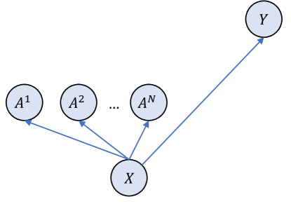
Figure 3: Independence illustration of observation phase with Bayesian network

Therefore, according to total probability theorem, Equation 5 and the above assumption, we derive:

$$P\left(y_{l},a_{i_{1}}^{1},a_{i_{2}}^{2},\dots,a_{i_{N}}^{N}\right)\\ \begin{aligned} &={\textstyle\sum_{k=1}^{n}}\left(P\left(y_{l},a_{i_{1}}^{1},a_{i_{2}}^{2},\dots,a_{i_{N}}^{N}\mid x_{k}\right)\cdot P(x_{k})\right)\\ &={\textstyle\sum_{k=1}^{n}}\left(P\left(y_{l}\mid x_{k}\right)\cdot{\textstyle\prod_{j=1}^{N}}P\left(a_{i_{j}}^{j}\mid x_{k}\right)\cdot P(x_{k})\right)\\ &=\frac{{\textstyle\sum_{k=1}^{n}\left(y_{l}(k)\cdot{\textstyle\prod_{j=1}^{N}}\alpha_{i_{j}}^{j}(k)\right)}}{n}\end{aligned}$$ (9)

Substitute Equation 8 and Equation 9 into Equation 7, we have:

$$P\left(y_{l}|a_{i_{1}}^{1},a_{i_{2}}^{2},\dots,a_{i_{N}}^{N}\right)=\frac{{\textstyle\sum_{k=1}^{n}\left(y_{l}(k)\cdot{\textstyle\prod_{j=1}^{N}}\alpha_{i_{j}}^{j}(k)\right)}}{{\textstyle\sum_{k=1}^{n}\left({\textstyle\prod_{j=1}^{N}}\alpha_{i_{j}}^{j}(k)\right)}}$$ (10)

Where it can be proved,

$${\textstyle\sum_{l=1}^{m}}P\left(y_{l}\mid a_{i_{1}}^{1},a_{i_{2}}^{2},\dots,a_{i_{N}}^{N}\right)=1$$ (11)

3.4 Inference Phase

Given $A^{j}$, with Equation 10 (passed experience) label $y_{l}$ can be inferred, this inferred $y_{l}$ has no pointing to any specific sample $x_{k}$, incl. also new input sample $x_{n+1}$, see Figure 4. So we can have following assumption:

Assumption 3.4.

Given $A^{j}$, $X$ and $Y$ is mutually independent in inference phase, $j=1,2,\dots,N$.

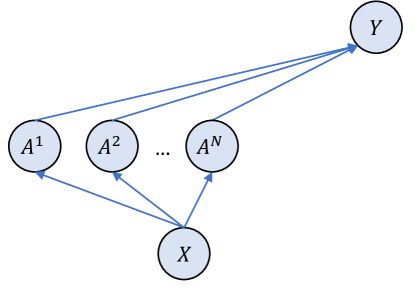
Figure 4: Independence illustration of inference phase with Bayesian network

Therefore, given a new input sample $X=x_{n+1}$, according to total probability theorem over joint sample space $\left(a_{i_{1}}^{1},a_{i_{2}}^{2},\dots,a_{i_{N}}^{N}\right)\in\mathbb{A}$, with 3.4, Equation 5 and Equation 10, we have:

$$P^{\mathbb{A}}\left(y_{l}\mid x_{n+1}\right)\\ \begin{aligned} &=\sum_{\mathbb{A}}\left(P\left(y_{l},a_{i_{1}}^{1},\dots,a_{i_{N}}^{N}\mid x_{n+1}\right)\right)\\ &=\sum_{\mathbb{A}}\left(P\left(y_{l}\mid a_{i_{1}}^{1},\dots,a_{i_{N}}^{N}\right)P\left(a_{i_{1}}^{1},\dots,a_{i_{N}}^{N}\mid x_{n+1}\right)\right)\\ &=\sum_{\mathbb{A}}\left(\frac{\sum_{k=1}^{n}\left(y_{l}(k){\prod_{j=1}^{N}}\alpha_{i_{j}}^{j}(k)\right)}{\sum_{k=1}^{n}\left({\prod_{j=1}^{N}}\alpha_{i_{j}}^{j}(k)\right)}\prod_{j=1}^{N}\alpha_{i_{j}}^{j}(n+1)\right)\end{aligned}$$ (12)

And the maximum posterior is the predicted label of an input sample:

$$\hat{y}:={\underset{l\in\left\{1,2,\dots,m\right\}}{\arg\max}\,P^{\mathbb{A}}\left(y_{l}\mid x_{n+1}\right)}$$ (13)

3.5 Discussion

Our proposed theory is derived based on three our proposed conditional mutual independency assumptions, see 3.2 3.3 and 3.4. However, in our opinion, these assumptions can neither be proved nor falsified, and we do not find any exceptions until now. Since this theory can not be mathematically proved, we can only validate it through experiment.

Finally, our proposed indeterminate probability theory is an extension of classical probability theory, and classical probability theory is one special case to our theory. More details to understand our theory, see Appendix A.

4 Training

4.1 Training Strategy

Given an input sample $x_{t}$ from a mini batch, with a minor modification of Equation 12:

$$P^{\mathbb{A}}\left(y_{l}\mid x_{t}\right)\\ \begin{aligned} &=\sum_{\mathbb{A}}\left(\dfrac{\sum_{k=b\cdot t_{0}+1}^{b\cdot t_{1}}\left(y_{l}(k){\prod_{j=1}^{N}}\alpha_{i_{j}}^{j}(k)\right)}{\sum_{k=b\cdot t_{0}+1}^{b\cdot t_{1}}\left({\prod_{j=1}^{N}}\alpha_{i_{j}}^{j}(k)\right)}\prod_{j=1}^{N}\alpha_{i_{j}}^{j}(t)\right)\\ &\approx\sum_{\mathbb{A}}\left(\frac{\max(H+h(t1),\epsilon)}{\max(G+g(t1),\epsilon)}\cdot{\prod_{j=1}^{N}}\alpha_{i_{j}}^{j}(t)\right)\end{aligned}$$ (14)

Where $b$ is for batch size, $t_{0}=\max(0,t_{1}-T)$, $t_{1}=\left\lceil\frac{t}{b}\right\rceil,t=1,2,\dots,n$. Hyper-parameter T is for forgetting use, i.e., $H$ and $G$ are calculated from the recent T batches. Hyper-parameter T is introduced because at beginning of training phase the calculated result with Equation 10 is not good yet. And the $\epsilon$ on the denominator is to avoid dividing zero, the $\epsilon$ on the numerator is to have an initial value of 1. Besides,

$$h(t1)={\textstyle\sum_{k=b\cdot(t_{1}-1)+1}^{b\cdot t_{1}}}\left(y_{l}(k)\cdot{\textstyle\prod_{j=1}^{N}}\alpha_{i_{j}}^{j}(k)\right)$$ (15)

$$g(t1)={\textstyle\sum_{k=b\cdot(t_{1}-1)+1}^{b\cdot t_{1}}}\left({\textstyle\prod_{j=1}^{N}}\alpha_{i_{j}}^{j}(k)\right)$$ (16)

$$H={\textstyle\sum_{k=\max(1,t_{1}-T)}^{t_{1}-1}}h(k),\text{for }t_{1}=2,3,\dots$$ (17)

$$G={\textstyle\sum_{k=\max(1,t_{1}-T)}^{t_{1}-1}}g(k),\text{for }t_{1}=2,3,\dots$$ (18)

Where $H$ and $G$ are not needed for gradient updating during back-propagation.

We use cross entropy as loss function:

$$\mathcal{L}=-{\textstyle\sum_{l=1}^{m}}\left(y_{l}(k)\cdot\log P^{\mathbb{A}}\left(y_{l}\mid x_{t}\right)\right)$$ (19)

The detailed algorithm implementation is shown in Algorithm 1.

Algorithm 1 IPNN training

Input: A sample $x_{t}$ from mini-batch
Parameter: Split shape, forget number $T$, $\epsilon$, learning rate $\eta$.
Output: The posterior $P^{\mathbb{A}}\left(y_{l}\mid x_{t}\right)$

1:  Declare default variables: $H,G,hList,gList$

2:  for $i=1,2,\dots$ Until Convergence do

3:     Compute $h,g$ with Equation 15 and Equation 16

4:     Record: $hList.append(h),gList.append(g)$

5:     if $i>T$ then

6:        Forget: $H=H-hList[0],G=G-gList[0]$

7:        Remove first element from $hList,gList$

8:     end if

9:     Compute posterior with Equation 14: $P^{\mathbb{A}}\left(y_{l}\mid x_{t}\right)$

10:     Compute loss with Equation 19: $\mathcal{L}(\theta)$

11:     Update model parameter: $\theta=\theta-\eta\nabla\mathcal{L}(\theta)$

12:     Update for next loop: $H=H+h,G=G+g$

13:  end for

14:  return model and the posterior

With Equation 14 we can get that $P^{\mathbb{A}}\left(y_{l}\mid x_{1}\right)=1$ for the first input sample if $y_{l}$ is the ground truth and batch size is 1. Therefore, for IPNN the loss may increase at the beginning and fall back again while training.

4.2 Multi-degree Classification (Optional)

In IPNN, the model outputs N different random variables $A^{1},A^{2},\dots,A^{N}$, if we use part of them to form sub-joint sample spaces, we are able of doing sub classification task, the sub-joint spaces are defined as $\Lambda^{1}\subset\mathbb{A},\Lambda^{2}\subset\mathbb{A},\dots$ The number of sub-joint sample spaces is:

$$\sum_{j=1}^{N}\binom{N}{j}=\sum_{j=1}^{N}\left(\frac{N!}{j!(N-j)!}\right)$$ (20)

If the input samples are additionally labeled for part of sub-joint sample spaces, defined as $Y^{\tau}\in\{y_{1}^{\tau},y_{2}^{\tau},\dots,y_{m^{\tau}}^{\tau}\}$. The sub classification task can be represented as $\left\langle X,\Lambda^{1},Y^{1}\right\rangle,\left\langle X,\Lambda^{2},Y^{2}\right\rangle,\dots$ With Equation 19 we have,

$$\mathcal{L}^{\tau}=-{\textstyle\sum_{l=1}^{m^{\tau}}}\left(y_{l}^{\tau}(k)\cdot\log P^{\Lambda^{\tau}}\left(y_{l}^{\tau}\mid x_{t}\right)\right),\tau=1,2,\dots$$ (21)

Together with the main loss, the overall loss is $\mathcal{L}+\mathcal{L}^{1}+\mathcal{L}^{2}+\dots$ In this way, we can perform multi-degree classification task. The additional labels can guide the convergence of the joint sample spaces and speed up the training process, as discussed later in Section 5.2.

4.3 Multi-degree Unsupervised Clustering

If there are no additional labels for the sub-joint sample spaces, the model are actually doing unsupervised clustering while training. And every sub-joint sample space describes one kind of clustering result, we have Equation 20 number of clustering situations in total.

4.4 Designation of Joint Sample Space

As in Appendix B proved, we have following proposition:

Proposition 4.1.

IPNN converges to global minimum only when $P\left(y_{l}|a_{i_{1}}^{1},a_{i_{2}}^{2},\dots,a_{i_{N}}^{N}\right)=1,\text{ for }\prod_{j=1}^{N}\alpha_{i_{j}}^{j}(t)>0,i_{j}=1,2,\dots,M_{j}$. In other word, each joint sample point corresponds to an unique category. However, a category can correspond to one or more joint sample points.

Corollary 4.2.

The necessary condition of achieving the global minimum is when the split shape defined in Equation 1 satisfies: ${\textstyle\prod_{j=1}^{N}}M_{j}\geq m$, where $m$ is the number of classes. That is, for a classification task, the number of all joint sample points is greater than the classification classes.

Besides, the unsupervised clustering (Section 4.3) depends on the input sample distributions, the split shape shall not violate from multi-degree clustering. For example, if the main attributes of one dataset shows three different colors, and your split shape is $\{M_{1}=2,M_{2}=2,\dots\}$, this will hinder the unsupervised clustering, in this case, the shape of one random variable is better set to 3. And as in Appendix C also analyzed, there are two local minimum situations, improper split shape will make IPNN go to local minimum.

In addition, the latter part from Proposition 4.1 also implies that IPNN may be able of doing further unsupervised classification task, this is beyond the scope of this discussion.

5 Experiments and Results

To evaluate the effectiveness of the proposed approach, we conducted experiments on MNIST (Deng, 2012) and a self-designed toy dataset.

5.1 Unsupervised Clustering

As in Section 4.3 discussed, IPNN is able of performing unsupervised clustering, we evaluate it on MNIST. The split shape is set to $\{M_{1}=2,M_{2}=10\}$, it means we have two random variables, and the first random variable is used to divide MNIST labels $0,1,\dots 9$ into two clusters. The cluster results is shown in Figure 5.

We find only when $\epsilon$ in Equation 14 is set to a relative high value that IPNN prefers to put number 1,4,7,9 into one cluster and the rest into another cluster, otherwise, the clustering results is always different for each round training. The reason is unknown, our intuition is that high $\epsilon$ makes that each category catch the free joint sample point more harder, categories have similar attributes together will be more possible to catch the free joint sample point.

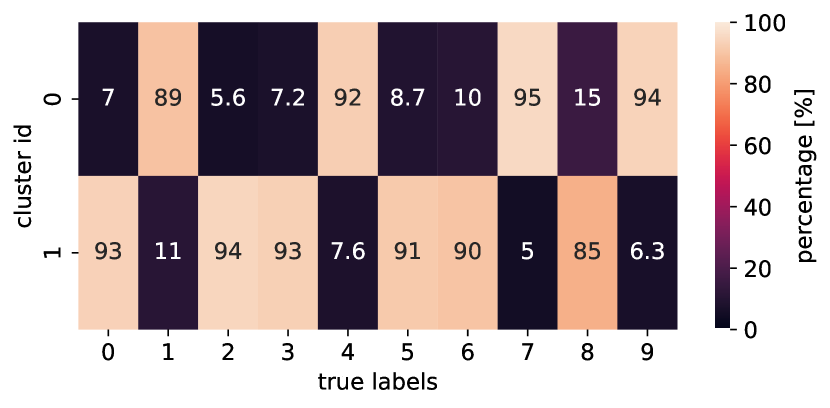
Figure 5: Unsupervised clustering results on MNIST: $\epsilon=2$, batch size $b=64$, forget number $T=5$, epoch is 5 per round. The test was repeated for 876 rounds with same configuration (different random seeds) in order to check the stability of clustering performance, each round clustering result is aligned using Jaccard similarity (Raff & Nicholas, 2017), the percentage is calculated with Equation 22.

$$\frac{1}{round}\cdot\sum_{i=1}^{round}\frac{\begin{matrix}\text{ number of samples with label }l\\ \text{ in one cluster at }i^{th}\text{ round}\end{matrix}}{\text{number of samples with label }l}$$ (22)

5.2 Avoiding Local Minimum with Multi-degree Classification

Another experiment is designed by us to check the performance of multi-degree classification (see Section 4.2): classification of binary vector into decimal value. The binary vector is the model inputs from ‘000000000000’ to ‘111111111111’, which are labeled from 0 to 4095. The split shape is set to $\{M_{1}=2,M_{2}=2,\dots,M_{12}=2\}$, which is exactly able of making a full classification. Besides, model weights are initialized as uniform distribution of $[-0.3,0.3]$, as discussed in Appendix C.

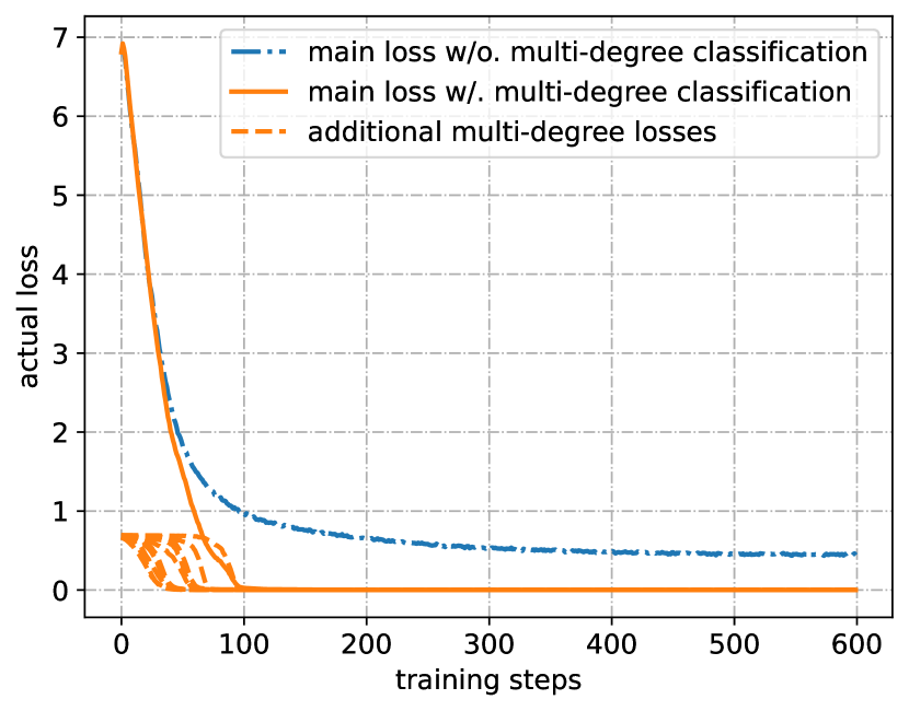
Figure 6: Loss of multi-degree classification of ‘binary to decimal’ on train dataset. Input samples are additionally labeled with $Y^{i}\in\{0,1\}$ for $i^{th}$ bit is 0 or 1, respectively. $Y^{i}$ corresponds to sub-joint sample space $\Lambda^{i}$ with split shape $\{M_{i}=2\},i=1,2,\dots 12$. Batch size is 4096, forget number $T=5,\enspace\epsilon=10^{-6}$.

The result is shown in Figure 6, IPNN without multi degree classification goes to local minimum with only $69.5\%$ train accuracy. We have only additionally labeled for 12 sub-joint spaces, and IPNN goes to global minimum with $100\%$ train accuracy.

Therefore, with only ${\textstyle\sum_{1}^{12}}2=24$ output nodes, IPNN can classify 4096 categories. Theoretically, if model with 100 output nodes are split into 10 equal parts, it can classify 10 billion categories. Hence, compared with the classification model with only one ‘softmax’ function, IPNN has no computationally expensive problems (see Section 1).

5.3 Hyper-parameter Analysis

IPNN has two import hyper-parameters: split shape and forget number T. In this section, we have analyzed it with test on MNIST, batch size is set to 64, $\epsilon=10^{-6}$. As shown in Figure 7, if the number of joint sample points (see Equation 3) is smaller than 10, IPNN is not able of making a full classification and its test accuracy is proportional to number of joint sample points, as number of joint sample points increases over 10, IPNN goes to global minimum for both 3 cases, this result is consistent with our analysis. However, we have exceptions, the accuracy of split shape with $\{M_{1}=2,M_{2}=5\}$ and $\{M_{1}=2,M_{2}=6\}$ is not high. From Figure 5 we know that for the first random variable, IPNN sometimes tends to put number 1,4,7,9 into one cluster and the rest into another cluster, so this cluster result request that the split shape need to be set minimums to $\{M_{1}=2,M_{2}\geq 6\}$ in order to have enough free joint sample points. That’s why the accuracy of split shape with $\{M_{1}=2,M_{2}=5\}$ is not high. (For $\{M_{1}=2,M_{2}=6\}$ case, only three numbers are in one cluster.)

Another test in Figure 8 shows that IPNN will go to local minimum as forget number T increases and cannot go to global minimum without further actions, hence, a relative small forget number T shall be found with try and error.

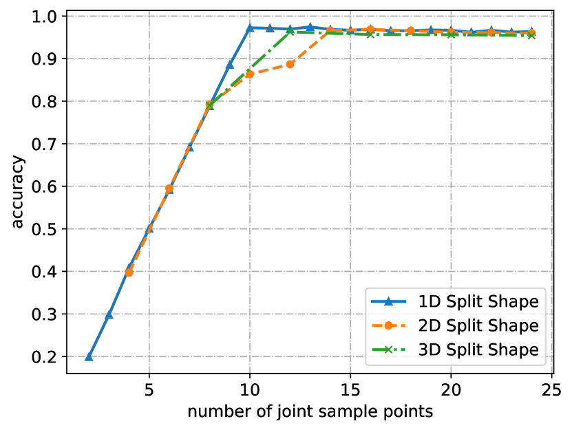
Figure 7: Impact Analysis of split shape with MNIST: accuracy on test dataset. 1D split shape is for $\{M_{1}=\tau\},\tau=2,3,\dots,24$. 2D split shape is for $\{M_{1}=2,M_{2}=\tau\},\tau=2,3,\dots,12$. 3D split shape is for $\{M_{1}=2,M_{2}=2,M_{3}=\tau\},\tau=2,3,\dots,6$. The x-axis is the number of joint sample points calculated with Equation 3.

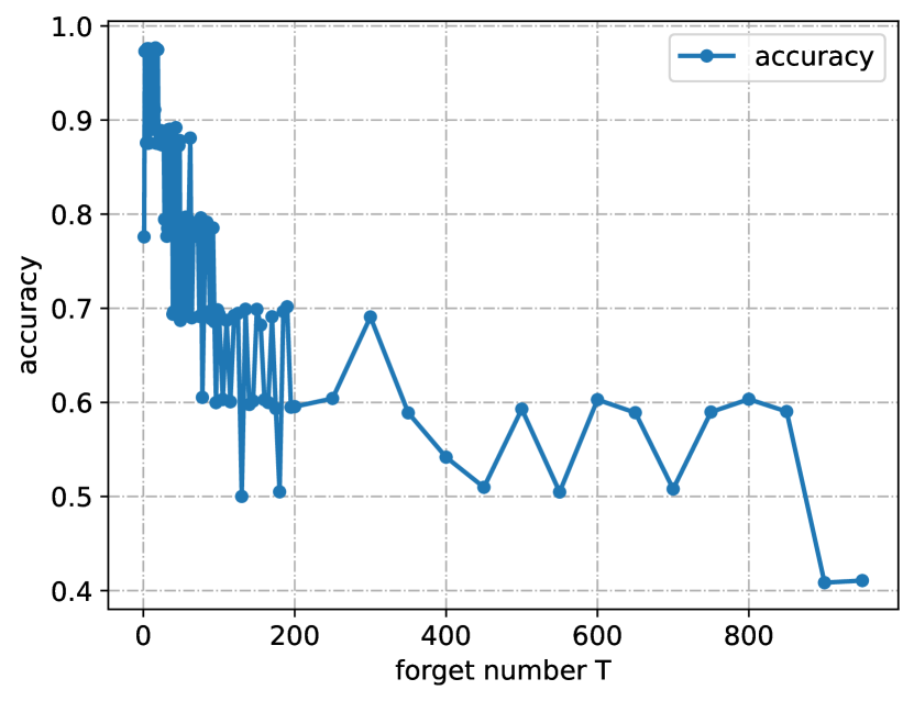
Figure 8: Impact Analysis of forget number T with MNIST: accuracy on test dataset. Split shape is $\{M_{1}=10\}$.

6 Conclusion

For a classification task, we proposed an approach to extract the attributes of input samples as random variables, and these variables are used to form a large joint sample space. After IPNN converges to global minimum, each joint sample point will correspond to an unique category, as discussed in Proposition 4.1. As the joint sample space increases exponentially, the classification capability of IPNN will increase accordingly.

We can then use the advantages of classical probability theory, for example, for very large joint sample space, we can use the Bayesian network approach or mutual independence among variables (see Appendix D) to simplify the model and improve the inference efficiency, in this way, a more complex Bayesian network could be built for more complex reasoning task.

Appendix A An Intuitive Explanation

Our most important contribution is that we propose a new general tractable probability Equation 12, rewritten here again:

$$P^{\mathbb{A}}\left(Y=y_{l}\mid X=x_{n+1}\right)=\\ \underset{\text{Inference phase}}{\underbrace{\sum_{\mathbb{A}}\left(\underset{\text{Observation phase}}{\underbrace{\frac{{\textstyle\sum_{k=1}^{n}}\left({\textstyle P\left(Y=y_{l}\mid X=x_{k}\right)\cdot\prod_{j=1}^{N}}P\left(A^{j}=a_{i_{j}}^{j}\mid X=x_{k}\right)\right)}{{\textstyle\sum_{k=1}^{n}}\left({\textstyle\prod_{j=1}^{N}}P\left(A^{j}=a_{i_{j}}^{j}\mid X=x_{k}\right)\right)}}}\cdot\prod_{j=1}^{N}P\left(A^{j}=a_{i_{j}}^{j}\mid X=x_{n+1}\right)\right)}}$$ (23)

Where X is random variable and $X=x_{k}$ denote the $k^{th}$ random experiment (or model input sample $x_{k}$), $Y$ and $A^{j}$ are different random variables, for more reading symbols, see Appendix E.

Since our proposed indeterminate probability theory is quite new, we will explain this idea by comparing it with classical probability theory, see below table:

Table 6: An intuitive comparison between classical probability theory and our proposed theory.

Classical	Observation	$P\left(Y=y_{l}\mid A^{j}=a_{i_{j}}^{j}\right)=\frac{\text{number of event }(Y=y_{l},A^{j}=a_{i_{j}}^{j})\text{ occurs}}{\text{number of event }(A^{j}=a_{i_{j}}^{j})\text{ occurs}}$
	Inference	$X=x_{n+1}\xrightarrow[\textbf{Determinate}]{P\left(A^{j}=a_{i_{j}}^{j}\mid X=x_{n+1}\right)=1}A^{j}=a_{i_{j}}^{j}\xrightarrow[\text{infer}]{P\left(Y=y_{l}\mid A^{j}=a_{i_{j}}^{j}\right)}Y=y_{l}$
Ours	Observation	$P\left(Y=y_{l}\mid A^{j}=a_{i_{j}}^{j}\right)=\frac{\text{sum of event }(Y=y_{l},A^{j}=a_{i_{j}}^{j})\text{ occurs, in decimal}}{\text{sum of event }(A^{j}=a_{i_{j}}^{j})\text{ occurs, in decimal}}$
	Inference	$X=x_{n+1}\to\left\{\begin{matrix}\xrightarrow[]{P\left(A^{j}=a_{1}^{j}\mid X=x_{n+1}\right)\in[0,1]}&A^{j}=a_{1}^{j}&\xrightarrow[]{P\left(Y=y_{l}\mid A^{j}=a_{1}^{j}\right)}\\ \xrightarrow[]{P\left(A^{j}=a_{2}^{j}\mid X=x_{n+1}\right)\in[0,1]}&A^{j}=a_{2}^{j}&\xrightarrow[]{P\left(Y=y_{l}\mid A^{j}=a_{2}^{j}\right)}\\ \xrightarrow[]{\dots}&A^{j}=\dots&\xrightarrow[]{\dots}\\ \xrightarrow[\textbf{Indeterminate}]{P\left(A^{j}=a_{M_{j}}^{j}\mid X=x_{n+1}\right)\in[0,1]}&A^{j}=a_{M_{j}}^{j}&\xrightarrow[\text{infer}]{P\left(Y=y_{l}\mid A^{j}=a_{M_{j}}^{j}\right)}\end{matrix}\right\}\to Y=y_{l}$
Note: Replacing $A^{j}$ with joint random variable $(A^{1},A^{2},\dots,A^{N})$ is also valid for above explanation.

In other word, for classical probability theory, perform a random experiment $X=x_{k}$, the event state is Determinate (happened or not happened), the probability is calculated by counting the number of occurrences, we define this process here as observation phase. For inference, perform a new random experiment $X=x_{n+1}$, the state of $A^{j}=a_{i_{j}}^{j}$ is Determinate again, so condition on $X=x_{n+1}$ is equivalent to condition on $A^{j}=a_{i_{j}}^{j}$, that may be the reason why condition on $X=x_{n+1}$ is not discussed explicitly in the past.

However, for our proposed indeterminate probability theory, perform a random experiment $X=x_{k}$, the event state is Indeterminate (understood as partly occurs), the probability is calculated by summing the decimal value of occurrences in observation phase. For inference, perform a new random experiment $X=x_{n+1}$, the state of $A^{j}=a_{i_{j}}^{j}$ is Indeterminate again, each case contributes the inference of $Y=y_{l}$, so the inference shall be the summation of all cases. Therefore, condition on $X=x_{n+1}$ is now different with condition on $A^{j}=a_{i_{j}}^{j}$, we need to explicitly formulate it, see Equation 23.

Once again, our proposed indeterminate probability theory does not have any conflict with classical probability theory, the observation and inference phase of classical probability theory is one special case to our theory.

Appendix B Global Minimum Analysis

Proof of Proposition 4.1.

Equation 12 can be rewritten as:

$$P^{\mathbb{A}}\left(y_{l}\mid x_{t}\right)=\sum_{\mathbb{A}}\left(p_{\mathbb{A}}\cdot{\textstyle\prod_{j=1}^{N}\alpha_{i_{j}}^{j}(t)}\right)$$ (24)

Where,

$$p_{\mathbb{A}}=P\left(y_{l}\mid a_{i_{1}}^{1},a_{i_{2}}^{2},\dots,a_{i_{N}}^{N}\right)$$ (25)

Theoretically, model converges to global minimum when the train and test loss is zero (Li & Yuan, 2017), and for the ground truth $y_{l}(t)=1$, with Equation 19 we have:

$$\sum_{\mathbb{A}}\left(p_{\mathbb{A}}\cdot{\textstyle\prod_{j=1}^{N}\alpha_{i_{j}}^{j}(t)}\right)=1$$ (26)

Subtract the above equation from Equation 6 gives:

$$\sum_{\mathbb{A}}\left((1-p_{\mathbb{A}})\cdot\prod_{j=1}^{N}\alpha_{i_{j}}^{j}(t)\right)=0$$ (27)

Because $\prod_{j=1}^{N}\alpha_{i_{j}}^{j}(t)\in[0,1]$ and $(1-p_{\mathbb{A}})\in[0,1]$, The above equation is then equivalent to:

$$p_{\mathbb{A}}=1,\text{ for }\prod_{j=1}^{N}\alpha_{i_{j}}^{j}(t)>0,i_{j}=1,2,\dots,M_{j}.$$ (28)

∎

Appendix C Local Minimum Analysis

Equation 24 can be further rewritten as:

$$P^{\mathbb{A}}\left(y_{l}\mid x_{t}\right)=\sum_{i_{\tau}=1}^{M_{\tau}}\left(\alpha_{i_{\tau}}^{\tau}(t)\cdot\sum_{\Lambda}\left(p_{\mathbb{A}}\cdot{\textstyle\prod_{j=1,j\neq\tau}^{N}\alpha_{i_{j}}^{j}(t)}\right)\right)\\ ={\textstyle\sum_{i_{\tau}=1}^{M_{\tau}}\left(\alpha_{i_{\tau}}^{\tau}(t)\cdot p_{i_{\tau}}\right)}$$ (29)

Where $\Lambda=(A^{1},\dots,A^{j},\dots,A^{N})\subset\mathbb{A},j\neq\tau$ and,

$$p_{i_{\tau}}={\sum_{\Lambda}\left(p_{\mathbb{A}}\cdot{\textstyle\prod_{j=1,j\neq\tau}^{N}\alpha_{i_{j}}^{j}(t)}\right)}$$ (30)

Substitute Equation 29 into Equation 19, and for the ground truth $y_{l}(t)=1$ the loss function can be written as:

$$\mathcal{L}=-\log({\textstyle\sum_{i_{\tau}=1}^{M_{\tau}}\left(\alpha_{i_{\tau}}^{\tau}(t)\cdot p_{i_{\tau}}\right)})$$ (31)

Let the model output before softmax function be $z_{i_{j}}$, we have:

$$\alpha_{i_{\tau}}^{\tau}(t)=\frac{e^{z_{i_{\tau}}}}{{\textstyle\sum_{i_{j}=1}^{M_{j}}e^{z_{i_{j}}}}}$$ (32)

In order to simplify the calculation, we assume $p_{\mathbb{A}}$ defined in Equation 25 is constant during back-propagation. so the gradient is:

$$\frac{\partial\mathcal{L}}{\partial z_{i_{\tau}}}=-\frac{\alpha_{i_{\tau}}^{\tau}(t)\cdot{\textstyle\sum_{i_{j}=1,i_{j}\neq i_{\tau}}^{M_{j}}}\left(e^{z_{i_{j}}}\cdot(p_{i_{\tau}}-p_{i_{j}})\right)}{\sum_{i_{j}=1}^{M_{j}}\left(e^{z_{i_{j}}}\cdot p_{i_{j}}\right)}$$ (33)

Therefore, we have two kind of situations that the algorithm will go to local minimum:

$$\frac{\partial\mathcal{L}}{\partial z_{i_{\tau}}}=\begin{cases}\to 0,&\text{if }\left|z_{i_{\tau}}-z_{i_{j}}\right|\to\infty\\ 0,&\text{if }p_{i_{\tau}}=p_{i_{j}}\\ Nonezero,&o.w.\end{cases}$$ (34)

Where $i_{\tau}=1,2,\dots,M_{\tau}$.

The first local minimum usually happens when Corollary 4.2 is not satisfied, that is, the number of joint sample points is smaller than the classification classes, the results are shown in Figure 7.

If the model weights are initialized to a very small value, the second local minimum may happen at the beginning of training. In such case, all the model output values are also small which will result in $\alpha_{1}^{j}(t)\approx\alpha_{2}^{j}(t)\approx\dots\approx\alpha_{M_{j}}^{j}(t)$, and it will further lead to all the $p_{i_{\tau}}$ be similar among each other. Therefore, if the model loss reduces slowly at the beginning of training, the model weights is suggested to be initialized to an relative high value. But the model weights shall not be set to too high values, otherwise it will lead to first local minimum.

As shown in Figure 9, if model weights are initialized to uniform distribution of $\left[-10^{-6},10^{-6}\right]$, its convergence speed is slower than the model weights initialized to uniform distribution of $\left[-0.3,0.3\right]$. Besides, model weights initialized to uniform distribution of $\left[-3,3\right]$ get almost stuck at local minimum and cannot go to global minimum. This result is consistent with our analysis.

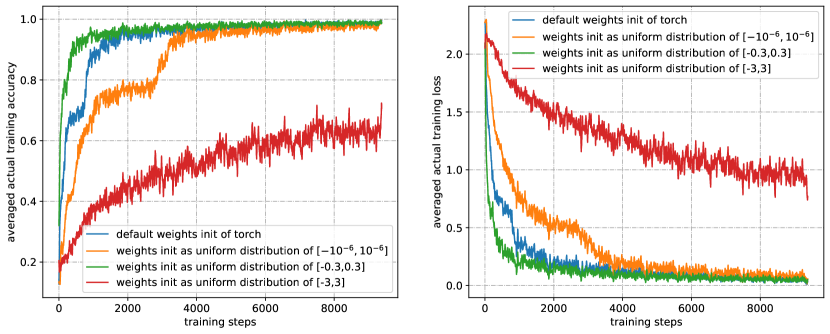
Figure 9: Model weights initialization impact analysis on MNIST. Split shape is $\{M_{1}=2,M_{2}=10\}$, batch size is 64, forget number $T=5,\enspace\epsilon=10^{-6}$.

Appendix D Mutual Independency

If we want the random variables $A^{1},A^{2},\dots,A^{N}$ partly or fully mutually independent, we can use their mutual information as loss function:

$$\mathcal{L}^{*}=KL\left(P(A^{1},A^{2},\dots,A^{N}),\prod_{j=1}^{N}P(A^{j})\right)=\sum_{\mathbb{A}}\left(P\left(a_{i_{1}}^{1},\dots,a_{i_{N}}^{N}\right)\cdot\log\frac{P\left(a_{i_{1}}^{1},\dots,a_{i_{N}}^{N}\right)}{\prod_{j=1}^{N}P(a_{i_{j}}^{j})}\right)$$ (35)

$$=\sum_{\mathbb{A}}\left(\frac{{\textstyle\sum_{k=1}^{n}}\left({\textstyle\prod_{j=1}^{N}}\alpha_{i_{j}}^{j}(k)\right)}{n}\cdot\log\left(\frac{\frac{{\textstyle\sum_{k=1}^{n}}\left({\textstyle\prod_{j=1}^{N}}\alpha_{i_{j}}^{j}(k)\right)}{n}}{\textstyle\prod_{j=1}^{N}\frac{{\textstyle\sum_{k=1}^{n}\alpha_{i_{j}}^{j}(k)}}{n}}\right)\right)$$

Appendix E Symbols

Table 7: Reading Symbols

Symbol	Meaning
$x_{k}$	input sample, $k=1,2,\dots,n$
$y_{l}$	output label, $l=1,2,\dots,m$
$A^{j}$	random variable, $j=1,2,\dots,N$
$a_{i_{j}}^{j}$	event of $A^{j},i_{j}=1,2,\dots,M_{j}$
$\mathbb{A}$	joint sample space
$\Lambda$	sub-joint sample space

References

- Biederman (1987) Biederman, I. Recognition-by-components: a theory of human image understanding. In Psychological review, pp. 115–147, 1987. doi: 10.1037/0033-295X.94.2.115.
- Cao (2010) Cao, Y. Study of the bayesian networks. In 2010 International Conference on E-Health Networking Digital Ecosystems and Technologies (EDT), volume 1, pp. 172–174, 2010. doi: 10.1109/EDT.2010.5496612.
- Deng (2012) Deng, L. The mnist database of handwritten digit images for machine learning research [best of the web]. IEEE Signal Processing Magazine, 29(6):141–142, 2012. doi: 10.1109/MSP.2012.2211477.
- Devlin et al. (2019) Devlin, J., Chang, M.-W., Lee, K., and Toutanova, K. Bert: Pre-training of deep bidirectional transformers for language understanding. ArXiv, abs/1810.04805, 2019.
- Fu et al. (2018) Fu, Y., Xiang, T., Jiang, Y.-G., Xue, X., Sigal, L., and Gong, S. Recent advances in zero-shot recognition: Toward data-efficient understanding of visual content. IEEE Signal Processing Magazine, 35(1):112–125, 2018. doi: 10.1109/MSP.2017.2763441.
- He et al. (2016) He, K., Zhang, X., Ren, S., and Sun, J. Deep residual learning for image recognition. In 2016 IEEE Conference on Computer Vision and Pattern Recognition (CVPR), pp. 770–778, 2016. doi: 10.1109/CVPR.2016.90.
- Kingma & Welling (2014) Kingma, D. P. and Welling, M. Auto-encoding variational bayes. CoRR, abs/1312.6114, 2014.
- Kocadağlı & Aşıkgil (2014) Kocadağlı, O. and Aşıkgil, B. Nonlinear time series forecasting with bayesian neural networks. Expert Systems with Applications, 41(15):6596–6610, 2014. ISSN 0957-4174. doi: https://doi.org/10.1016/j.eswa.2014.04.035. URL https://www.sciencedirect.com/science/article/pii/S0957417414002589.
- Lampert et al. (2009) Lampert, C. H., Nickisch, H., and Harmeling, S. Learning to detect unseen object classes by between-class attribute transfer. In 2009 IEEE Conference on Computer Vision and Pattern Recognition, pp. 951–958, 2009. doi: 10.1109/CVPR.2009.5206594.
- Li & Yuan (2017) Li, Y. and Yuan, Y. Convergence analysis of two-layer neural networks with relu activation. In Proceedings of the 31st International Conference on Neural Information Processing Systems, NIPS’17, pp. 597–607, Red Hook, NY, USA, 2017. Curran Associates Inc. ISBN 9781510860964.
- Mohammed & Umaashankar (2018) Mohammed, A. A. and Umaashankar, V. Effectiveness of hierarchical softmax in large scale classification tasks. In 2018 International Conference on Advances in Computing, Communications and Informatics (ICACCI), pp. 1090–1094, 2018. doi: 10.1109/ICACCI.2018.8554637.
- Morales & Yu (2021) Morales, J. and Yu, W. Improving neural network’s performance using bayesian inference. Neurocomputing, 461:319–326, 2021. ISSN 0925-2312. doi: https://doi.org/10.1016/j.neucom.2021.07.054. URL https://www.sciencedirect.com/science/article/pii/S0925231221011309.
- Raff & Nicholas (2017) Raff, E. and Nicholas, C. An alternative to ncd for large sequences, lempel-ziv jaccard distance. In Proceedings of the 23rd ACM SIGKDD International Conference on Knowledge Discovery and Data Mining, KDD ’17, pp. 1007–1015, New York, NY, USA, 2017. Association for Computing Machinery. ISBN 9781450348874. doi: 10.1145/3097983.3098111. URL https://doi.org/10.1145/3097983.3098111.
- Su & Chou (2006) Su, C. and Chou, C.-J. A neural network-based approach for statistical probability distribution recognition. Quality Engineering, 18:293 – 297, 2006.
- Vaswani et al. (2017) Vaswani, A., Shazeer, N., Parmar, N., Uszkoreit, J., Jones, L., Gomez, A. N., Kaiser, L., and Polosukhin, I. Attention is all you need. In Proceedings of the 31st International Conference on Neural Information Processing Systems, NIPS’17, pp. 6000–6010, Red Hook, NY, USA, 2017. Curran Associates Inc. ISBN 9781510860964.