Sparse Iso-FLOP Transformations for Maximizing Training Efficiency

Abstract

Recent works have explored the use of weight sparsity to improve the training efficiency (test accuracy w.r.t training FLOPs) of deep neural networks (DNNs). These works aim to reduce training FLOPs but training with sparse weights often leads to accuracy loss or requires longer training schedules, making the resulting training efficiency less clear. In contrast, we focus on using sparsity to increase accuracy while using the same FLOPs as the dense model and show training efficiency gains through higher accuracy. In this work, we introduce Sparse-IFT, a family of Sparse Iso-FLOP Transformations which are used as drop-in replacements for dense layers to improve their representational capacity and FLOP efficiency. Each transformation is parameterized by a single hyperparameter (sparsity level) and provides a larger search space to find optimal sparse masks. Without changing any training hyperparameters, replacing dense layers with Sparse-IFT leads to significant improvements across computer vision (CV) and natural language processing (NLP) tasks, including ResNet-18 on ImageNet (+3.5%) and GPT-3 Small on WikiText-103 (-0.4 PPL), both matching larger dense model variants that use 2x or more FLOPs. To our knowledge, this is the first work to demonstrate the use of sparsity for improving the accuracy of dense models via a simple-to-use set of sparse transformations. Code is available at: https://github.com/CerebrasResearch/Sparse-IFT.

Cerebras Systems

1 Introduction

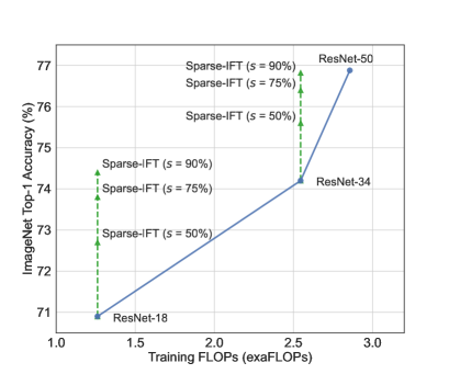
Figure 1: Accuracy vs. Training FLOPs for different variants of ResNet on ImageNet. Sparse Iso-FLOP Transformation (Sparse-IFT) provides significant accuracy gains across different models and sparsity levels while using the same FLOP budget as its dense counterpart. In particular, the best Sparse-IFT variants of ResNet-18 and ResNet-34 achieve 3.5% and 2.7% improvements over their dense baselines, respectively.

Increases in model size and training data have led to many breakthroughs in deep learning (e.g., AlexNet (Krizhevsky et al., 2012), ResNet (He et al., 2016), Transformers (Vaswani et al., 2017), GPT (Radford et al., 2018, 2019), AlphaGo (Silver et al., 2017), etc.). Consequently, the computational and memory footprint of training and deploying deep neural networks (DNNs) has grown exponentially. To enable the deployment of large models, multiple techniques (e.g., distillation (Hinton et al., 2015), quantization (Han et al., 2015a), pruning (Han et al., 2015b)) have been introduced to reduce inference FLOPs and memory requirements. While these techniques improve inference efficiency (test accuracy w.r.t inference FLOPs), the associated training costs are still prohibitive. In this work, we focus on improving the training efficiency (test-accuracy w.r.t training FLOPs) of DNNs.

Recent works (Evci et al., 2020; Jayakumar et al., 2020) have explored using weight sparsity to reduce the FLOPs spent in training. Frankle & Carbin (2018) demonstrate that sparse subnetworks (termed “lottery tickets”) exist at initialization and can be trained to match the accuracy of their original dense network. Inspired by this result, various dynamic sparse training (DST) methods (Ma et al., 2022; Evci et al., 2020; Liu et al., 2021a; Jayakumar et al., 2020) attempt to find optimal sparse subnetworks in a single training run. While these methods primarily aim to improve training efficiency by reaching dense accuracy with fewer FLOPs, they often perform worse than their dense baselines or rely on longer training schedules (up to 2-5$\times$ training iterations) to close the gap. As a result, these techniques can sometimes even require more FLOPs than training the dense model (Ma et al., 2022; Evci et al., 2020; Jayakumar et al., 2020). In contrast to prior work, we focus on showing training efficiency gains by using sparsity to increase accuracy while consuming the same training FLOPs as the dense model. Specifically, we introduce a family of Sparse Iso-FLOP Transformations (Sparse-IFT) that can be used as drop-in replacements for dense layers in DNNs. These transformations increase the representational capacity of layers and facilitate the discovery of optimal sparse subnetworks without changing the layer’s underlying FLOPs (i.e., Iso-FLOP). For example, making a layer wider but sparser increases dimensionality while still maintaining FLOPs due to sparsity. All Sparse-IFT members are parameterized by a single hyperparameter, the sparsity level. Figure 1 summarizes the ImageNet performance with ResNet models, where our Sparse Wide IFT variants significantly increase the accuracy of matching Iso-FLOP dense models. In particular, Sparse Wide ResNet-18 at 90% sparsity improves the top-1 accuracy from 70.9% to 74.4% (+3.5%), and outperforms a dense ResNet-34 (74.2%) while using 2x fewer FLOPs. We emphasize that these gains were obtained by replacing dense layers with Sparse-IFTs and required no changes to training hyperparameters. The main contributions of our work are:

1. We introduce a family of Sparse Iso-FLOP Transformations to improve the training efficiency of DNNs by improving accuracy while holding FLOPs constant. These transformations are parameterized by a single hyperparameter (sparsity level) and can be used as drop-in replacements for dense layers without changing the overall FLOPs of the model.

2. In the CV domain, using Sparse-IFT increases the top-1 accuracy of ResNet-18 and ResNet-34 by 3.5% and 2.6% respectively on ImageNet. Finetuning these pre-trained models for object detection (MS COCO) and segmentation (CityScapes) leads to an improvement of 5.2% mAP and 2.4% mIoU, respectively.

3. In the NLP domain, using Sparse-IFT with GPT-3 Small leads to a 0.4 perplexity improvement on the WikiText-103 language modeling task.

4. We report wall-clock speed-ups for both training on the Cerebras CS-2 (Lie, 2022a, b) and inference on a CPU with unstructured sparsity, highlighting the practical value of Sparse-IFT.

2 Method

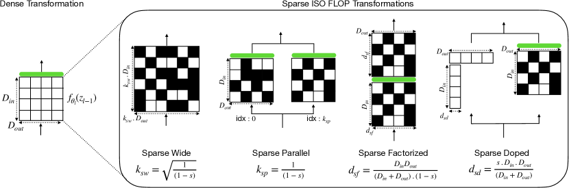
Figure 2: Different members of the Sparse-IFT family. Transformation of all members is parameterized by a single hyperparameter (i.e., sparsity level ($s$)). Black and white squares denote sparse and active weights, respectively. Green block indicates a non-linear activation function (e.g., BatchNorm, ReLU, LayerNorm). All transformations are derived with sparsity set to $50\%$ as an example, are Iso-FLOP to the dense feedforward function $f_{\theta_{l}}$, and hence can be used as a drop-in replacement of $f_{\theta_{l}}$. As shown in the figure, FLOPs spent in a dense matrix multiplication can be utilized to enhance the representational capacity of the feedforward function using unstructured sparsity. See Section 2.4 for more details about each member.

In this section, we present our method to improve training efficiency. We first explain our intuition and hypotheses, followed by our methodology.

2.1 Training with Dense Matrices is FLOP Inefficient

Prior works have shown that modern DNNs are overparameterized and that the features and weights learned at each layer are sparse. Recent work of Lottery Ticket Hypothesis (LTH) (Frankle & Carbin, 2018) demonstrates that sparse DNNs can be trained to the same accuracy as their dense counterparts, as long as one seeds the training with a good sparsity mask (termed as “lottery ticket”). These works indicate that the optimal set of weights in a DNN is sparse. Therefore, representing these weights as dense matrices throughout training is FLOP inefficient, and training with sparse matrices should be more efficient. However, in practice, most sparse training methods obtain worse accuracy than dense baseline. We hypothesize that this is due to the inefficiency of searching for “lottery tickets” within a single training run.

While sparse models reduce the FLOPs needed per step, we hypothesize that existing sparse training methods make sub-optimal use of these computational savings. For example, state-of-the-art (SOTA) sparse training methods (Jayakumar et al., 2020; Evci et al., 2020) invest these FLOP savings into longer training schedules to close the accuracy gap and compensate for the inability to discover an optimal mask earlier in training. This setup is inefficient since it ultimately requires more training FLOPs than the dense baseline to reach the same target accuracy. In our work, we take an orthogonal approach and invest these FLOP savings into (a) increasing the representational capacity of a layer and (b) increasing its search space, which we hypothesize can facilitate the discovery of an optimal sparse mask (Ramanujan et al., 2020; Stosic & Stosic, 2021). We do this by replacing dense transformations with FLOP-equivalent sparse transformations. We denote these transformations as the Sparse Iso-FLOP Transformation (Sparse-IFT) family.

2.2 Setup

For clarity, we will explain our method for a fully connected neural network. In Appendix A.1, we detail the straightforward extension of our method to convolutional layers. Let $\mathcal{N}$ denote a $L$ layered DNN parameterized by $\Theta_{\mathcal{N}}$. Let $\Theta_{\mathcal{N}}\in\{\theta_{1},...,\theta_{L}\}$ denote the parameters of the DNN. The output of the $l$-th layer is defined as: $z_{l}=\sigma(f_{\theta_{l}}(z_{l-1}))$ for some activation function $\sigma$ (e.g., ReLU (Nair & Hinton, 2010)) and feedforward function $f_{\theta_{l}}$. Specifically, let $f_{\theta_{l}}(z_{l-1})=\theta_{l}^{T}z_{l-1}$, where $\theta_{l}\in\mathbb{R}^{D_{in}\times D_{out}}$, $z_{l-1}\in\mathbb{R}^{D_{in}\times B}$ and $B$, $D_{in}$, $D_{out}$ denote the batch-size, input, and output dimensionality of features respectively. The total FLOPs needed for $f_{\theta_{l}}$ are given by $B{\cdot}D_{in}{\cdot}D_{out}$.

2.3 Sparse Iso-FLOP Transformations

In the standard setup, the feedforward function $f_{\theta_{l}}$ computes the output features as a linear transformation of input features. From a theoretical perspective, the feedforward function can make use of arbitrary non-linear transformations. However, in practice, most transformations are expressed as dense matrix multiplications due to widespread support on GPUs (Nvidia, 2023).

As stated before, we are interested in improving the training efficiency of DNNs, by enhancing the representational capacity of the feedforward function. Naively increasing the representational capacity by stacking more layers (Lin et al., 2014a), increasing width (Zagoruyko & Komodakis, 2016), mixture of experts (Shazeer et al., 2016), etc. increases the computational FLOPs. In our work, we use unstructured sparsity in weight matrices and ensure that the FLOPs of the transformation are the same as that of a dense feedforward function. Let $\Psi_{l}$ denote the set of Sparse Iso-FLOP Transformations (Sparse-IFT) for a particular layer $l$:

$$\Psi_{l}:\{\psi_{l}(s),0\leq s<1,g(\psi_{l})\approx g(f_{\theta_{l}})\},$$

where $\psi_{l}$ is a transformation, $s$ represents the sparsity level, and $g(.)$ returns the computational FLOPs. Each transformation in this set satisfies the following properties: (1) the computational FLOPs of the transformation $\psi_{l}$ are same as that of dense transformation $f_{\theta_{l}}$, and (2) the transformation is parameterized by a single hyperparameter - the sparsity level. Since these transformations are Iso-FLOP to the dense feedforward function, we can use them as drop-in replacements without affecting the FLOPs of a layer. While many FLOP-equivalent transformations fall under the Sparse-IFT family, in this work, we detail four different members: Sparse Wide, Sparse Parallel, Sparse Factorized, and Sparse Doped.

2.4 Members of Sparse-IFT

Sparse Wide

The sparse wide transformation augments the representational capacity of a layer by increasing the number of output features while keeping $s$ fraction of weights sparse. When using this transformation, we widen the input and output features for all the $L$ layers of the network with the same widening factor, $k_{sw}$, to avoid a mismatch in feature dimensionality across layers. Let $\theta_{l}^{sw}\in\mathbb{R}^{k_{sw}{\cdot}D_{in}\times k_{sw}{\cdot}D_{out}}$ denote the transformation matrix, with $s$ fraction of weights being sparse. Since the fraction of non-sparse weights is given by $1-s$, the FLOPs required by this transformation are $B{\cdot}(k_{sw}{\cdot}D_{in}){\cdot}(k_{sw}{\cdot}D_{out}){\cdot}(1-s)$. Setting these equal to the FLOPs of the original dense $f_{\theta_{l}}$, we obtain the widening factor $k_{sw}=\sqrt{\frac{1}{(1-s)}}$. If we set the sparsity $s$ to $0$, we obtain $k_{sw}$ as $1$ and recover the original dense feedforward function.

Sparse Parallel

The sparse parallel transformation replaces the feedforward function with a sum of $k_{sp}$ non-linear functions. Let $\theta_{l}^{sp}\in\{\theta_{l}^{sp,1},...,\theta_{l}^{sp,k_{sp}}\}$ denote the parameters of this transformation, where $\theta_{l}^{sp,j}\in\mathbb{R}^{D_{in}\times D_{out}}$ denotes the transformation matrix of $j^{th}$ function, where $s$ fraction of weights are sparse. The sparse parallel transformation in this case is $\psi^{sp}_{l}=\sum^{k_{sp}}_{j=1}\sigma((\theta_{l}^{sp,j})^{T}z_{l})$, where $\sigma$ is a non linear function. In practice, $\psi^{sp}_{l}$ is implemented as a layer with $k_{sp}$ parallel branches. The computational FLOPs of this transformation is $k_{sp}{\cdot}B{\cdot}D_{in}{\cdot}D_{out}{\cdot}(1-s)$. Setting these FLOPs equal to FLOPs of $f_{\theta}$, we obtain $k_{sp}=\frac{1}{(1-s)}$. Note, at $s=0$, the number of parallel branches $k_{sp}$ is $1$. If we replace the non-linear function $\sigma$ with Identity, we can recover the original dense feedforward transformation.

Sparse Factorized

The transformation matrix of the feedforward function $f_{\theta_{l}}$ is denoted by $\theta_{l}\in\mathbb{R}^{D_{in}\times D_{out}}$. Multiple works have explored matrix factorization techniques to express the transformation matrix $\theta_{l}$ as a product of two matrices $\theta_{l}=UV^{T}$, where $U\in\mathbb{R}^{D_{in}\times d}$, $V\in\mathbb{R}^{D_{out}\times d}$. Khodak et al. (2020); Tai et al. (2016) and Chen et al. (2021b) have explored low-rank factorization ($d<<D_{out}$) as a form of structured sparsity to improve training and inference efficiency, while Arora et al. (2018) and Guo et al. (2020a) have explored overparameterized factorizations for better generalization and faster convergence. In contrast, we use factorization to augment the representational capacity without decreasing or increasing the FLOPs. More precisely, let $\theta_{l}^{sf}\in\{U_{l},V_{l}\}$ denote the parameters of this transformation, where $U_{l}\in\mathbb{R}^{D_{in}\times d_{sf}}$, $V_{l}\in\mathbb{R}^{d_{sf}\times D_{out}}$ are sparse matrices with $s$ fraction of their weights being sparse. The functional transformation in this case is $\psi^{sf}_{l}=V_{l}^{T}\sigma(U_{l}^{T}z_{l})$. The computational FLOPs of this transformation is $d_{sf}{\cdot}B{\cdot}(D_{in}+D_{out}){\cdot}(1-s)$. Setting these FLOPs equal to FLOPs of $f_{\theta_{l}}$, we obtain $d_{sf}=\frac{D_{in}{\cdot}D_{out}}{(D_{in}+D_{out}){\cdot}(1-s)}$. Note, setting sparsity $s=0$, we recover a non-linear low-rank factorization with dense matrices.

Sparse Doped

family of transformation is inspired by works (Chen et al., 2021a; Thakker et al., 2021; Udell & Townsend, 2019; Candès et al., 2011) which approximate a dense matrix with a combination of low-rank factorization and sparse matrix. In our work, we replace the feedforward function with low-rank factorization (with rank $d_{sd}$) and an unstructured sparse weight matrix (with sparsity $s$). Let $U_{l}\in\mathbb{R}^{D_{in}\times d_{sd}},V_{l}\in\mathbb{R}^{d_{sd}\times D_{out}}$ denote the low-rank matrices, and $\theta_{l}^{sd}\in\mathbb{R}^{D_{in}\times D_{out}}$ denote the matrix with unstructured sparsity. The functional transformation, in this case, is given by $\psi^{sd}_{l}=V_{l}^{T}(U_{l}^{T}z_{l})+\sigma((\theta_{l}^{sd})^{T}z_{l})$. The computational FLOPs associated with this transformation are $B{\cdot}d_{sd}{\cdot}(D_{in}+D_{out})+(1-s){\cdot}B{\cdot}D_{in}{\cdot}D_{out}$. Setting these FLOPs equal to FLOPs of $f_{\theta_{l}}$, we obtain $d_{sd}=\frac{s{\cdot}D_{in}{\cdot}D_{out}}{(D_{in}+D_{out})}$. Note, as $s\to 0$ and $d_{sd}\to 0$, the low-rank component of the transformation disappears, and we can recover the dense feedforward function as a special case by setting $\sigma$ to Identity.

2.5 Cardinality of Search Space

One of our hypotheses is that increasing the search space of the sparsity mask via Sparse-IFT can make training more efficient. Results from past work support this hypothesis. Ramanujan et al. (2020) demonstrate that the odds of finding a lottery ticket in a randomly initialized network increase with the width of a network. Liu et al. (2022b) and Stosic & Stosic (2021) show that increasing the search space by increasing width or depth improves accuracy. In our work, we define the cardinality of a search space as the number of weights a sparse training method can explore. Table 1 characterizes the cardinality of search space for each member of the Sparse-IFT family. The search space for Sparse Wide, Sparse Parallel, and Sparse Factorized transformations increase proportional to the width scaling factor, number of parallel branches, and size of intermediate hidden dimension, respectively. Sparse Doped transformation splits its computational FLOPs between low-rank factorization and unstructured sparse weight matrix. The size of the unstructured weight matrix is invariant to sparsity; thus cardinality of search space for this transformation is constant.

Table 1: Cardinality of search space of sparsity mask for different members of the Sparse-IFT family.

Transformation	Cardinality of Search Space
Sparse Wide	$(k_{sw})^{2}{\cdot}(D_{in}{\cdot}D_{out})$
Sparse Parallel	$k_{sp}{\cdot}(D_{in}{\cdot}D_{out})$
Sparse Factorized	$d_{sf}{\cdot}(D_{in}+D_{out})$
Sparse Doped	$D_{in}{\cdot}D_{out}$

3 Experiments 

In this section, we demonstrate how transformations from the Sparse-IFT Family lead to improvements across a variety of different tasks in the CV and NLP domains. First, in section 3.2, we describe the experimental setups and validate the design choices through multiple ablation studies on CIFAR-100 (Krizhevsky et al., 2009), followed by results on ImageNet (Krizhevsky et al., 2012). Then, in section 3.5, we highlight the advantages of pre-training with Sparse-IFT through gains on downstream tasks. Next, we present the benefits of Sparse-IFT in the NLP domain by demonstrating results on BERT (Devlin et al., 2018) and GPT (Brown et al., 2020) in section 3.6. Finally in section 4, we show speed-ups during training and inference with unstructured sparsity, measured in wall clock time. Unless stated otherwise, the results presented below are obtained by replacing all dense layers with a given transformation from the Sparse-IFT family while only tuning the sparsity level. All sparse models are trained using a uniform sparsity distribution (i.e., all layers have the same sparsity level). We adopt the default hyperparameters from RigL (Evci et al., 2020) for dynamic sparsity. More details about the setup can be found in Appendix B.2.

3.1 CV Implementation Details

We evaluate our method on CIFAR-100 and ImageNet using convolutional networks and hybrid Vision Transformer (ViT) networks. We follow published training settings for CIFAR-100 (DeVries & Taylor, 2017) and ImageNet (Nvidia, 2019b). For both datasets, we follow the standard evaluation procedures and report the top-1 accuracy. Details for model architectures, datasets, and training hyperparameters are given in Appendix B.2.

3.2 Results and Ablations on CIFAR-100

In this section, we conduct various ablations to validate our design choices. Unless stated otherwise, all experiments below are with ResNet-18 architecture on CIFAR-100.

Table 2: Evaluation of Sparse Wide IFT using various sparse training methods with ResNet-18 on CIFAR-100 across different values of sparsity (columns). Best accuracy for each sparse training method is highlighted in bold.

Dense	Sparse Training Method	0.50	0.75	0.90
77.0 $\pm$ 0.2	Static	78.5	78.3	78.2
	SET	78.8	79.2	79.8
	RigL	79.1	79.5	80.1

Importance of Dynamic Sparsity

All members of the Sparse-IFT family utilize transformations with unstructured sparsity. This study investigates the importance of the sparse training method when training different configurations of Sparse-IFT architectures. For this analysis, we focus on the Sparse Wide transformation and evaluate it with transformations obtained with sparsity $\in$ {50%, 75%, 90%} using three sparse training methods: static sparsity, SET (Mocanu et al., 2018) and RigL (Evci et al., 2020). RigL and SET are dynamic sparse training methods in which the sparsity mask evolves during training. The key difference is that RigL updates the mask based on gradient information, whereas SET updates the mask randomly. Results of our ablation are documented in Table 2. Here, the following trends can be observed: 1) the Sparse Wide transformation outperforms dense baselines across all operating points (sparsity and sparse training method), 2) dynamic sparse training methods (RigL and SET) obtain higher accuracies compared to training with static sparsity, and 3) gains with static sparsity plateau at lower levels of sparsity, while dynamic sparse training methods gain accuracy at higher sparsities. As mentioned in Section 2.5, Sparse-IFT transformations increase the search space $\propto$ sparsity. Dynamic sparse training methods can explore and exploit this increased search space (Stosic & Stosic, 2021) and therefore outperform training with static sparsity. Out of the two dynamic sparse training methods evaluated in our study, RigL consistently outperforms SET. Therefore, we use RigL as our sparse training method for all the experiments reported below.

Importance of Using Non-Linear Activations

Some of the Sparse-IFTs are inspired by recent works which overparameterize the feedforward function during training and fold it back into a single dense matrix post training (Ding et al., 2021b, a; Guo et al., 2020a; Ding et al., 2019). Although these works show the benefits of linear overparameterization, this comes at the cost of a significant increase in training FLOPs. In contrast, while we also increase the representational capacity of the feedforward function, we do so with an Iso-FLOP transformation. Since we remain Iso-FLOP to the original dense model, we do not require post-training modifications to collapse weight matrices for inference efficiency. This uniquely allows us to use non-linearities (e.g., ReLU) in our Sparse-IFTs to enhance the representational capacity of the network further. We validate the importance of this design choice by training ResNet-18 with Sparse Factorized IFT with and without non-linearities, and observe significant accuracy gains across all sparsity levels when using non-linear activations. For example, at 90% Sparse Factorized, using non-linearity, we see a 1.8% gain in test accuracy over the ResNet-18 CIFAR-100 dense baseline, compared to a drop of 0.5% without it. These findings hold for other members of the Sparse-IFT family as well (see Appendix B.1 for more details).

Table 3: Evaluation of Sparse-IFTs on CIFAR-100 with ResNet-18 model across different values of sparsity (columns). Best accuracy of each transformation is highlighted in bold. All members of the Sparse-IFT family outperform the dense baseline by a significant margin.

Dense	Transformation	0.50	0.75	0.90
77.0 $\pm$ 0.2	Sparse Wide	79.1	79.5	80.1
	Sparse Factorized	77.8	78.4	78.9
	Sparse Parallel	77.9	79.1	78.2
	Sparse Doped	78.2	77.8	76.9

Sparse-IFT with ResNet-18

In the preceding paragraphs, we validate the design choices for our method (i.e., the importance of dynamic sparsity and non-linearity). Now, we evaluate different members of the Sparse-IFT family on ResNet-18 and CIFAR-100 across different sparsity levels. Table 3 highlights the best accuracy achieved by each member of the Sparse-IFT family. Compared to the accuracy of the dense baseline (77%), all Sparse-IFT members obtain significant accuracy improvements using the same FLOPs as the dense model. We note that the Sparse Doped transformation is the only Sparse-IFT which does not gain accuracy at higher levels of sparsity. We hypothesize that this phenomenon occurs due to two reasons: 1) cardinality of the search space of the sparsity mask does not increase with sparsity level (see Table 1), and 2) the number of active weights in the unstructured matrix decreases $\propto$ sparsity.

Comparison with Structured Sparsity

In this section, we compare structured sparsity to unstructured sparsity with Sparse-IFT. In theory, for a fixed number of non-zero elements in a sparse mask, the use of unstructured sparsity can search over all the possible variations of the mask. However, since most hardware accelerators are not able to accelerate computations with unstructured sparsity, multiple works have investigated training with structured sparsity (e.g., low-rank and block-sparse matrices) to obtain wall clock speed-ups (Khodak et al., 2020; Tai et al., 2016; Chen et al., 2021b; Hubara et al., 2021; Dao et al., 2022; Chen et al., 2022a). We study structured sparsity by deriving Iso-FLOP configurations using low-rank and block sparsity with Sparse Wide transformation. We use the method proposed in Hubara et al. (2021) to search N:M transposable sparsity, which can accelerate training on GPUs with Tensor Cores. In our evaluation, the low-rank factorization results were worse than block sparsity (see more details in Appendix B.3.2). Table 4 compares unstructured sparsity to block sparsity. Although using Sparse-IFT with block sparse matrices lead to improvements over the dense baseline, unstructured sparsity achieves the highest gains. This result can be explained by the fact that block-sparse matrices have reduced mask diversity (Hubara et al., 2021) compared to unstructured sparse matrices.

Table 4: Evaluation of Sparse Wide IFT with unstructured and structured sparsity across different values of sparsity (columns) on CIFAR-100 with ResNet-18.

Dense	Sparsity Pattern	0.50	0.75	0.90
77.0 $\pm$ 0.2	Unstructured	79.1	79.5	80.1
	N:M Block Sparse	77.1	78.4	78.1

Table 5: Evaluation of Sparse Wide IFT with various compute efficient architectures on CIFAR-100 across different values of sparsity (columns). Using Sparse Wide IFT, all architectures outperform the dense by a significant margin.

	Dense	0.50	0.75
MobileNetV2	72.4 $\pm$ 0.2	73.4	73.7
MobileViT-S	73.5 $\pm$ 0.1	74.6	74.8
BotNet-50	79.8 $\pm$ 0.2	80.3	80.6

3.3 Results with Efficient Architectures

To further understand the robustness of Sparse-IFT across different model families, we evaluate Sparse-IFT on architectures that are optimized for efficient inference (MobileNetV2 (Sandler et al., 2018) and MobileViT (Mehta & Rastegari, 2021)) and efficient training (BotNet (Srinivas et al., 2021)). We transform the dense layers in these architectures with Sparse Wide IFT and evaluate them at different sparsity levels. We observe a noticeable increase in test accuracy across all architectures (see Table 5). In addition, we demonstrate the robustness of the Sparse-IFTs by also applying the Sparse Parallel transformation and show consistent improvement across all architectures (see Appendix B.3.1). We evaluate the best-performing architecture (BotNet-50) on ImageNet (see Section 3.4). The details of the experimental setup can be found in Appendix B.2.

3.4 Results on ImageNet

We take the best-performing Sparse-IFTs (i.e., Sparse Wide and Sparse Parallel) on CIFAR-100, and evaluate them on ImageNet using ResNet-18. Both families of Sparse-IFT obtain significantly higher accuracy compared to the dense baseline (refer to Table 6). Note, Sparse Wide IFT ResNet-18 at 90% sparsity improves over the dense baseline by 3.5%, and is able to match accuracy of dense ResNet34 with 2$\times$ fewer training FLOPs (see Figure 1). We take the best-performing transformation (Sparse Wide) and apply it to ResNet-34 and BotNet-50. Increasing sparsity leads to a consistent increase in accuracy, indicating improved training efficiency at higher sparsities across all architectures. On BotNet-50, a hybrid ViT model, we see a 1% improvement at 90% sparsity.

Table 6: Evaluation of Sparse-IFT on ImageNet. Best result for each transformation and architecture is highlighted in bold.

	Dense	Transformation	Sparsity
			0.50	0.75	0.90
ResNet-18	70.9 $\pm$ 0.1	Sparse Wide	72.7	73.8	74.4
		Sparse Parallel	72.7	73.2	74.0
ResNet-34	74.2 $\pm$ 0.1	Sparse Wide	75.6	76.4	76.8
BotNet-50	77.5 $\pm$ 0.1	Sparse Wide	77.9	78.3	78.5

3.5 Transfer Learning with Sparse-IFT

To show the effectiveness of pre-training our Sparse-IFT classification backbones, we evaluate them on 1) object detection on MS COCO 2017 (Lin et al., 2014b), and 2) semantic segmentation on CityScapes (Cordts et al., 2016). For object detection, we adopt the RetinaNet (Lin et al., 2017b) framework from the MMDetection open-source toolbox (Chen et al., 2019) and report results in the standardized training setting. For semantic segmentation, we utilize DeepLabV3+ (Chen et al., 2018) in the MMSegmenation open-source toolbox (Contributors, 2020). We evaluate ResNet-18 with Sparse Wide transformation (best-performing transformation on ImageNet). To ensure FLOP-equivalent comparisons with the dense backbone, we ensure that Sparse-IFT backbones remain sparse during fine-tuning. Appendix B.3.3 provides more details regarding the training setup. We summarize our findings in Table 7. Using Sparse Wide IFT ResNet-18 backbone leads to significant accuracy gains across all metrics on both downstream tasks.

Table 7: Evaluation of Sparse-IFT variants of ResNet-18 as backbones on downstream tasks : (a) Object detection on MS COCO, (b) Semantic segmentation on Cityscapes. Sparse Wide IFT ResNet-18 backbones outperform dense baseline by a significant margin across all metrics on both tasks.

	Metric	Dense	Sparsity
			0.50	0.75	0.90
MS COCO	AP	29.3	31.3	32.8	34.5
	AP50	46.2	49.0	51.0	53.5
	AP75	30.9	33.0	34.8	36.5
CityScapes	mIoU	76.7	77.9	78.9	79.1
	mAcc	84.4	85.1	85.7	86.0

Table 8: Evaluation of Sparse-IFT for pre-training GPT-3 Small from scratch on the WikiText-103 dataset and report the test perplexity (lower is better) over 3 random seeds.

	Dense	0.50	0.75
GPT-3 Small	20.8 $\pm$ 0.3	20.4	22.1

3.6 NLP Implementation Details

We evaluate Sparse-IFT by training GPT-3 Small (Brown et al., 2020) from scratch on the WikiText-103 (Merity et al., 2017) language modeling task, a commonly used NLP benchmark dataset. Training large GPT models is very costly and compute intensive. Although Sparse-IFT does not increase the training FLOPs, in practice, since GPUs do not accelerate unstructured sparsity, the wall clock time to train with Sparse-IFT increases $\propto\frac{1}{1-s}$. For example, training with 75% sparsity leads to 4x longer wall clock training time on GPUs. The compute cost and resources for training quickly become prohibitive when transforming GPT models with Sparse-IFT. Therefore, we believe Sparse-IFT is well suited for emerging sparse deep learning hardware accelerators like the Cerebras CS-2 (Lie, 2022a, b). Hence, we train our GPT models on the CS-2 and leverage its ability to accelerate training with unstructured sparsity. We provide more details about performance and wall clock speed-ups in Section 4. The current implementation of Cerebras CS-2’s specialized kernels support training with static unstructured sparsity; therefore, results in this section are reported without DST methods.

3.7 Results on GPT End-to-End Training

We train the Sparse Wide IFT GPT-3 Small models at 50% and 75% sparsity levels, and compare against the standard dense GPT-3 Small and GPT-3 Medium models. Following Dao et al. (2022), we train all models from scratch on the WikiText-103 dataset and report the average test perplexity (PPL) over 3 random seeds in Table 8. We show that Sparse Wide IFT GPT-3 Small at 50% sparsity improves the perplexity by 0.4 over its dense counterpart. This result is inline with dense GPT-3 Medium (20.5 ± 0.2 PPL) while our Sparse Wide IFT model uses 2.4x fewer training FLOPs. In Appendix C.1, we provide details on the hyperparameters and how the total training FLOPs for the models in Table 8 were calculated.

GPT Pre-training and Fine-tuning

While not the primary focus of our method, we note that Sparse-IFT can also be applied in a fine-tuning setup for NLP models. After pre-training sparse, the Sparse-IFT model can be fine-tuned as-is (i.e., remains sparse) or after densifying (i.e., allow the zeroed weights to learn) using a technique such as SPDF (Thangarasa et al., 2023). We perform some preliminary fine-tuning studies on BERT and GPT and those results can be found in Appendix C.2.

4 Wall Clock Acceleration with Sparsity

Results presented in Section 3 help validate our hypothesis, i.e., training DNNs with dense matrices is FLOP inefficient. Replacing dense layers with Sparse-IFT increases the training efficiency by providing significantly higher accuracy using the same amount of training FLOPS. This result is significant from a theoretical perspective but does not translate to direct practical value on hardware that can not accelerate unstructured sparsity (e.g., Nvidia GPUs, Google TPUs). However, there has recently been a renewed interest in hardware software co-design for accelerating unstructured sparsity. Here, we benchmark Sparse-IFT on these platforms to demonstrate its practical value. We hope these results motivate the broader machine learning community to explore and exploit the benefits of unstructured sparsity for training and inference.

Setup

We evaluate the inference efficiency of Sparse-IFT using Neural Magic’s sparsity-aware runtime. We benchmark different configurations of the Sparse Wide ResNet-18 model with sparsity $\in$ {50%, 75%, 90%} for batched inference on ImageNet. We also evaluate the training efficiency of Sparse-IFT on the Cerebras CS-2 which supports and accelerates training with unstructured sparsity. Technical details regarding the implementation of the specialized sparse kernels are beyond the scope of this paper. We plan to release our code and details about the hardware. We benchmark different configurations of Sparse Wide GPT-3 1.3B with sparsity $\in$ {50%, 75%, 90%} and report seconds/ iteration. More details about our setup can be found in Appendix D. Our benchmarking results are detailed in Figure 3. We note that configurations of Sparse-IFT at different values of sparsity do not incur a significant change in the FLOPs compared to the dense model. On ideal hardware, FLOPs should translate directly to wall clock time, and the inference latency or training time for all configurations of Sparse-IFT should be the same as that of the dense model (dotted black line). Conversely, when hardware does not support unstructured sparsity, the latency or training time of Sparse-IFT variants increases with sparsity (blue line). Our results lie between these two spectrums (green line). Using Neural Magic’s inference runtime, we observe significant speed-up with unstructured sparsity (5.2x at 90% sparsity). Similarly, we observe significant training speed-up (3.8x at 90% sparsity) on the Cerebras CS-2.

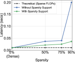
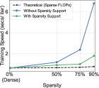
Figure 3: Benchmarking (left) inference on Neural Magic’s DeepSparse runtime and (right) training acceleration with unstructured sparsity on the Cerebras CS-2.

5 Related Work

Our work is similar to the body of work studying the role of overparameterization and sparsity for training DNNs. The modeling capacity needed to learn a task is often unknown. Hence, we often solve this by training overparameterized models to fully exploit the learning capability and then compress them into a smaller subnetwork.

Overparameterization

Nakkiran et al. (2021) show that DNNs benefit from overparameterization. Following this, there have been many works that leverage overparameterization by scaling the size of models (Rae et al., 2021; Goyal et al., 2022) and augmenting existing DNNs to increase modeling capacity and the accuracy of trained networks  (Guo et al., 2020b; Ding et al., 2019, 2021b; Cao et al., 2022; Vasu et al., 2022; Liu et al., 2022a). These methods use linear parameterizations of the model, making them highly inefficient to train, and are focused on improving inference throughput (reduced latency). In contrast, our work is focused on improving the modeling capacity using sparse non-linear parameterizations, which do not increase training FLOPs compared to the baseline model. While both approaches have the same inference FLOPs, our approach improves accuracy without increasing the training FLOPs.

Sparse Training

The Lottery Ticket Hypothesis (Frankle & Carbin, 2018; Frankle et al., 2020) shows that accurate sparse subnetworks exist in overparameterized dense networks but require training a dense baseline to find. Other approaches have proposed frameworks for identifying lottery tickets (Zhou et al., 2019; Ma et al., 2022) but still require a tremendous amount of compute resources. Following this, various attempts have been made to find the optimal sparse subnetwork in a single shot. These methods either try to find the subnetworks at initialization (Tanaka et al., 2020; Wang et al., 2020a; de Jorge et al., 2020; Lee et al., 2018) or dynamically during training (Mocanu et al., 2018; Evci et al., 2020; Jayakumar et al., 2020; Raihan & Aamodt, 2020). However, given a fixed model capacity, these methods tradeoff accuracy relative to the dense baseline to save training FLOPs.  Stosic & Stosic (2021) and Ramanujan et al. (2020) increase the search space during sparse training to retain accuracy; however, do not guarantee FLOPs savings. In contrast to these methods, our work introduces a set of non-linear sparse transformations, which increase the representational capacity of the network. This approach does not introduce a new sparse training algorithm, but instead improves the search space of existing methods, leading to improved generalization while being efficient to train.

Iso-Parameter vs. Iso-FLOP

Recent sparsity literature is focused on improving generalization at high sparsity levels. Hence, layer-wise sparsity distributions such as the Erdös-Rényi-Kernel (Evci et al., 2020), Ideal Gas Quota (Chen et al., 2022b), and parameter leveling (Golubeva et al., 2021) are often used with sparse training to boost accuracies. However, these works target the setting where the models being compared have a fixed parameter budget (i.e., Iso-Parameter), which does not translate to similar training FLOPs to the original dense model (especially in CNNs). As a result, training models with these distributions often require different memory or computational resources per layer. Our approach does not focus on this Iso-Parameter setting but instead adopts the uniform sparsity distribution (i.e., every layer gets the same sparsity level), ensuring uniform FLOP reductions across the network. We also ensure the same computational FLOPs of a dense network by leveraging sparsity along with our Iso-FLOP transformations.

6 Conclusion

We introduce a new family of Sparse Iso-FLOP Transformations (Sparse-IFT) to improve the training efficiency of DNNs. These transformations can be used as drop-in replacements for dense layers and increase the representational capacity while using sparsity to maintain training FLOPs. This increase in capacity also translates to a larger search space allowing sparse training methods to explore better and identify optimal sparse subnetworks. For the same computational cost as the original dense model, Sparse-IFT improves the training efficiency across multiple model families in the CV and NLP domains for various tasks. We hope our work will open new investigations into improving the accuracy of DNNs via sparsity, especially as new hardware accelerators build better support for weight sparsity during training.

7 Acknowledgements

We thank Anshul Samar and Joel Hestness for their helpful comments and edits that improved our manuscript. We also thank Kevin Leong for assisting on the Cerebras CS-2 GPT-3 experiments and Dylan Finch for performance evaluation on CS-2. Finally, we provide details on each author’s contributions in Appendix E.

Appendix A Additional Methodology Details

A.1 Sparse-IFT for Convolutional Layers

In this section, we detail the straightforward extension of the Sparse-IFT family for convolutional layers.

Sparse Wide

Similar to the setup for fully connected layers, in the case of convolutional layers, we widen the number of input and output channels.

Sparse Parallel

Similar to the setup for fully connected layers, in the case of convolutional layers, we can implement this transformation with the use of convolutional branches in parallel.

Sparse Factorized and Sparse Doped

Let $\theta_{l}\in\mathbb{R}^{c_{in}\times c_{out}\times k_{h}\times k_{w}}$ represent the weight matrix of a convolutional layer, where $c_{in},c_{out},k_{h},k_{w}$ denote the input channels, output channels, kernel height, and kernel width, respectively. We apply low-rank or matrix factorization to the weight matrix by first converting the 4D tensor into a 2D matrix with shape: $(c_{in}\cdot k_{h}\cdot k_{w})\times c_{out}$. In this setup, we can express $\theta_{l}=UV^{T}$, where $U\in\mathbb{R}^{c_{in}\cdot k_{h}\cdot k_{w}\times d}$, $V\in\mathbb{R}^{c_{out}\times d}$. In this factorization, $U$ learns a lower-dimensional set of features and is implemented as a convolutional layer with $d$ output channels and $k_{h}\times k_{w}$ filter. $V$ matrix expands this low-dimensional set of features and is implemented as a convolutional layer with $1\times 1$ filter.

A.1.1 Sparse-IFT for Depthwise Convolution Layers

For a normal convolution layer, all inputs are convolved to all outputs. However, for depthwise convolutions, each input channel is convolved with its own set of filters. Let $\theta_{l}\in\mathbb{R}^{c_{in}\times c_{out}\times k_{h}\times k_{w}}$ represent the weight matrix of a normal convolution layer, where $c_{in},c_{out},k_{h},k_{w}$ denote the input channels, output channels, kernel height, and kernel width, respectively. An equivalent depthwise convolution layer will have weights $\theta_{dw,l}\in\mathbb{R}^{1\times c_{out}\times k_{h}\times k_{w}}$.

Sparse Wide

A Sparse Wide depthwise convolution will have weights $\theta_{dw,l}^{sw}\in\mathbb{R}^{1\times k_{sw}{\cdot}c_{out}\times k_{h}\times k_{w}}$. Since the fraction of non-sparse weights is given by $1-s$, the FLOPs required by this transformation are $B{\cdot}(k_{sw}{\cdot}c_{out}){\cdot}k_{h}{\cdot}k_{w}{\cdot}(1-s)$. Setting these equal to the FLOPs of the original dense $\theta_{dw,l}$, we obtain the widening factor $k_{sw}=\frac{1}{(1-s)}$. In this case, we do not scale the input channels as it converts the depthwise convolution to a grouped convolution without an equivalent scaling in the number of groups.

Other Sparse-IFTs

The Sparse Wide transformation generally changes a layer’s input and output channels, subsequently scaling the following layers in a CNN. However, the other Sparse-IFTs (e.g., Sparse Parallel, Sparse Factorized, and Sparse Doped) do not modify a convolution layer’s input or output channels (as seen in Figure 2). This allows for fine-grained control of what layers to apply the Sparse-IFT transformations. Since depthwise convolutions are an extreme form of structured sparsity, where some filters interact with only specific input channels, we opt not to sparsify them when using the other Sparse-IFTs and leave the layer unchanged while still maintaining FLOPs equivalent to the dense baseline. Note that the different convolution layers surrounding the depthwise convolution are still transformed with Sparse-IFT to increase their representational capacity.

Appendix B Computer Vision: Experimental Settings

B.1 Importance of Non-linearity

We use BatchNorm (Ioffe & Szegedy, 2015) followed by ReLU (Nair & Hinton, 2010) as a non-linearity. We provide an extended set of empirical results in Table 9 to help validate the importance of training with and without non-linearity by training configurations of the Sparse Parallel, Factorized, and Doped IFTs at different levels of sparsity. The results without non-linear activation functions are often worse than the dense accuracy (77%) across all Sparse-IFT family transformations. We omit Sparse Wide in Table 9 because here we increase the number of channels in the convolutional layers while maintaining the existing architecture.

Table 9: Evaluation on the importance of utilizing the non-linear activation across different members of Sparse-IFT with ResNet-18 on CIFAR100 across different values of sparsity (columns). Non-linear activations enhance the representational capacity of Sparse-IFT, leading to higher accuracy. All reported results are the average over 3 random seeds.

Transformation	Non-linear activation	0.50	0.75	0.90
Sparse Factorized	✗	75.9 $\pm$ 0.3	76.6 $\pm$ 0.4	76.5 $\pm$ 0.4
	✓	77.8 $\pm$ 0.4	78.4 $\pm$ 0.5	78.9 $\pm$ 0.5
Sparse Parallel	✗	77.1 $\pm$ 0.1	77.2 $\pm$ 0.2	77.6 $\pm$ 0.1
	✓	77.9 $\pm$ 0.2	79.1 $\pm$ 0.2	78.2 $\pm$ 0.2
Sparse Doped	✗	77.3 $\pm$ 0.2	77.1 $\pm$ 0.1	76.5 $\pm$ 0.2
	✓	78.2 $\pm$ 0.1	77.8 $\pm$ 0.1	76.9 $\pm$ 0.2

B.2 Computer Vision: Pre-Training Settings

CIFAR-100

Our implementation of CIFAR-100 follows the setup from (DeVries & Taylor, 2017) for ResNets. We train the models for 200 epochs with batches of 128 using SGD, Nesterov momentum of 0.9, and weight-decay of 5$\times 10^{-4}$. The learning rate is initially set to 0.1 and is scheduled to decay to decrease by a factor of 5x after each of the 60th, 120th, and 160th epochs. Following recent advances in improving ResNets, we initialize the network with Kaiming He initialization (He et al., 2016), zero-init residuals (He et al., 2019), and disable weight-decay in biases and BatchNorm (Ioffe & Szegedy, 2015) layers. For CIFAR-100 experiments with MobileNetV2, MobileViT-S, and BotNet-50, we follow the same training setup used for ResNet, but the learning rate is scheduled via cosine annealing.

ImageNet

Our implementation of ImageNet follows the standard setup from (Krizhevsky et al., 2017; Simonyan & Zisserman, 2014). The image is resized with its shorter side randomly sampled in [256, 480] for scale augmentation (Simonyan & Zisserman, 2014). A 224 $\times$ 224 crop is randomly sampled from an image or its horizontal flop, and then normalized. For evaluation, the image is first resized to 256 $\times$ 256, followed by a 224 $\times$ 224 center crop, and then normalized. Following recent advances in improving ResNets, we initialize the network with Kaiming He initialization (He et al., 2016) and zero-init residuals (He et al., 2019).

For ResNets, we replicate the settings recommended by Nvidia (Nvidia, 2019b), which uses the SGD optimizer with a momentum of 0.875 and weight decay of 3.0517578125$\times 10^{-5}$. We disable weight-decay for biases and BatchNorm layers. The model is trained with label smoothing (Szegedy et al., 2016) of 0.1 and mixed precision (Micikevicius et al., 2018) for the standard 90 epochs using a cosine-decay learning rate schedule with an initial learning rate of 0.256 for a batch size of 256. Srinivas et al. (2021) follow the same setup as ResNet for training BotNet-50 on ImageNet, therefore we maintain the same hyperparameter settings as Nvidia (2019b) for our BotNet-50 ImageNet experiments.

Sparsity Setup

For enabling the Sparse-IFTs, we use the RigL (Evci et al., 2020) algorithm in its default hyperparameter settings ($\alpha=0.3,\Delta T=100$), with the drop-fraction ($\alpha$) annealed using a cosine decay schedule for 75% of the training run. We keep the first and last layers (input convolution and output linear layer) dense to prevent a significant degradation in model quality during pre-training, which is standard practice. We account for these additional dense FLOPs by increasing the sparsity in the remaining layers, similar to Gale et al. (2019) and Liu et al. (2022b).

B.3 Computer Vision

B.3.1 Sparse-IFT on Efficient Computer Vision Architectures

Here, we provide an extended set of results on MobileNetV2, MobileViT-S, and BotNet-50 on CIFAR-100. In particular, we enable Sparse Wide and Sparse Parallel IFT at 50% and 75% sparsity values (see Table 10).

Table 10: Evaluation of Sparse Wide and Sparse Parallel IFT with various compute efficient architectures on CIFAR-100 across different values of sparsity (columns). Using Sparse Parallel IFT, all architectures outperform the dense baseline by a significant margin.

	Dense	Transformation	0.50	0.75
MobileNetV2	72.4 $\pm$ 0.2	Sparse Wide	73.4	73.7
		Sparse Parallel	72.9	73.3
MobileViT-S	73.5 $\pm$ 0.1	Sparse Wide	74.6	74.8
		Sparse Parallel	73.7	74.4
BotNet-50	79.8 $\pm$ 0.2	Sparse Wide	80.3	80.6
		Sparse Parallel	79.7	80.5

B.3.2 Evaluation of Sparse-IFT with Structured Sparsity

Block Sparsity

For all of our N:M transposable sparsity experiments, we use the official code from Habana Labs . To derive Iso-FLOP configurations with block sparsity, we reuse the analysis done previously with unstructured sparsity (see Section 2.4) and express the width scaling as a function of sparsity. However, we will search for a block sparse mask during training instead of an unstructured sparsity mask. We use the method proposed by Hubara et al. (2021) to search N:M transposable sparsity, which can accelerate both the forward and backward pass during training on NVIDIA GPUs with Tensor Cores. We use 4:8-T, 2:8-T, and 1:8-T block patterns to obtain 50%, 75%, and 87.5% sparsity, respectively. Note the 1:8-T block is the closest approximation to a 90% sparsity pattern attainable with a block size of 8. We also set up and experimented using the method proposed by Jiang et al. (2022) to train with fine-grained sparse block structures dynamically. However, the algorithm uses agglomerative clustering which led to a much slower runtime and quickly ran out of memory even at 50% sparsity using the Sparse Wide transformation on a single Nvidia V100 (16 GB).

Low Rank

Let $k_{lr}$ be the factor with which we widen all layers’ input and output dimensions for low-rank factorization. We replace all dense layers with low-rank factorization, i.e. $\theta_{l}^{lr}=U_{l}V_{l}^{T}$, where $U_{l}\in\mathbb{R}^{(k_{lr}.D_{in})\times d}$ and $V_{l}\in\mathbb{R}^{(k_{lr}.D_{out})\times d}$. Given a widening factor and equating the FLOPs of this transformation to that of a dense transformation $f_{\theta}$, we obtain the following expression for rank $d$: $\frac{D_{in}.D_{out}.k_{lr}}{(D_{in}+D_{out}}$. We evaluate this factorization across different values of width-scaling $k_{lr}$ in Table 11.

Table 11: Comparison of structured sparse and unstructured sparse methods on CIFAR-100 test accuracy on ResNet-18.

			Width Scaling Factor
Transformation	Sparsity Type	Sparsity	1x	1.41x	2x	3.16x
Low Rank, Linear	Structured	0%	74.1	74.3	74.3	73.4
Low Rank, Non-Linear	Structured	0%	76.8	76.5	76.0	75.3
Sparse Wide	N:M Block Sparse (Hubara et al., 2021)	4:8-T		77.1
		2:8-T			78.4
		1:8-T				78.1
	Unstructured Sparse (Evci et al., 2020)	50%		79.1
		75%			79.5
		90%				80.1

B.3.3 Evaluation on downstream tasks

COCO Object Detection

This dataset contains 118K training, 5K validation (minival), and 20K test-dev images. We adopt the standard single-scale training setting (Lin et al., 2017a) where there is no additional data augmentation beyond standard horizontal flipping. For training and testing, the input images are resized so that the shorter edge is 800 pixels (Lin et al., 2017a). The model is trained with a batch size of 16, using the SGD optimizer with a momentum of 0.9 and weight decay of 1$\times 10^{-4}$. We follow the standard 1x schedule (12 epochs) using a step learning rate schedule, with a 10x decrease at epochs 8 and 11, an initial learning rate warmup of 500 steps starting from a learning rate of 2$\times 10^{-5}$, and a peak learning rate of 0.01.

Table 12: Object detection results on COCO minival in the RetinaNet framework. Sparse Wide IFT configurations of RetinaNet outperform the dense baseline by a large margin on all metrics while using similar FLOPs.

Backbone	AP	AP50	AP75	APS	APM	APL
Dense	29.3	46.2	30.9	14.7	31.5	39.6
Sparse Wide (50%)	31.3	49.0	33.0	16.6	34.0	42.0
Sparse Wide (75%)	32.8	51.0	34.8	17.3	35.8	43.3
Sparse Wide (90%)	34.5	53.5	36.5	18.6	37.6	45.3

CityScapes Semantic Segmenation

Setup

We follow the same training protocol as (Zhao et al., 2017), where the data is augmented by random cropping (from 1024 $\times$ 2048 to 512 $\times$ 1024), random scaling in the range [0.5, 2], and random horizontal flipping. The model is trained with a batch size of 16, using the SGD optimizer with a momentum of 0.9 and weight decay of 5$\times 10^{-4}$. We follow the 80K iterations setup from MMSegmentation with an initial learning rate of 0.01 annealed using a poly learning rate schedule to a minimum of 1$\times 10^{-4}$. Similar to most setups that tune hyperparameters (Zhao et al., 2017; Liu et al., 2021b; Wang et al., 2020b) for reporting the best results, we tune the learning rate for all our models. All our results are reported using a learning rate of 0.03 for the sparse backbones and 0.01 for the dense baseline.

Table 13: Semantic segmentation results on the Cityscapes val set using DeepLabV3+. Sparse Wide IFT configurations ResNet-18 backbones outperform the dense baseline on all metrics while using similar FLOPs.

Backbone	mIoU	mAcc
Dense	76.72	84.40
Sparse Wide (50%)	77.90	85.12
Sparse Wide (75%)	78.92	85.68
Sparse Wide (90%)	79.10	86.01

Appendix C Natural Language Processing: Experimental Settings 

C.1 Details for GPT End-to-End Training

Our end-to-end training setup for GPT-3 on WikiText-103 follows a similar procedure to Dao et al. (2022). We use a batch size of 512 and train with the AdamW optimizer for 100 epochs. Also, we use a learning rate warmup for 10 epochs and a weight decay of 0.1. To discover good hyperparameters, we perform a grid search to discover an appropriate learning rate among {8e-3, 6e-3, 5.4e-3, 1.8e-3, 6e-4, 2e-4, 6e-5} that led to the best perplexity for a given compute budget on the validation set. In Table 14, we outline the architecture configurations for the original dense model and its Sparse Wide IFT 50% and 75% variants.

Table 14: Sizes and architecture definitions of the dense GPT-3 Small model and its Sparse Wide IFT variants.

Model	Transformation	Sparsity	$n_{layers}$	$d_{model}$	$d_{\text{ff}}$	$n_{heads}$	$d_{head}$
GPT-3 Small	Dense	0%	12	768	3072	12	64
GPT-3 Small	Sparse Wide	50%	12	1092	4344	12	64
GPT-3 Small	Sparse Wide	75%	12	1536	6144	12	64

WikiText-103 End-to-End Training Results

We highlight that in Table 15, the Sparse Wide IFT GPT-3 Small at 50% sparsity attains a better perplexity on WikiText-103 while using 2.4x fewer training FLOPs than the GPT-3 Medium dense model. In this setup, using Sparse Wide transformation does not change the FLOP of the dense layer, but this leads to a slight increase in the attention FLOPs. This explains the 1.17x increase in FLOPs between the GPT-3 Small Sparse Wide at 50% sparsity and the dense GPT-3 Small model. Note, out of all the Sparse-IFTs, this increase only occurs in the Sparse Wide transformation.

Table 15: Details on the total training FLOPs for each GPT-3 model tested. We note that the reported FLOPs per sequence (seq) include both forward and backward passes. The reported perplexity (lower is better) is on the WikiText-103 test set over 3 random seeds.

Model	Transformation	Sparsity	Total Seqs	Total FLOPs/ Seq	Total FLOPs	Total exaFLOPs	Perplexity
GPT-3 Small	Dense	0%	2.28e6	8.763e11	2.0011e18	2.00	20.8 $\pm$ 0.3
GPT-3 Small	Sparse Wide	50%	2.28e6	1.029e12	2.3498e18	2.35	20.4 $\pm$ 0.2
GPT-3 Medium	Dense	0%	2.28e6	2.4845e12	5.6734e18	5.67	20.5 $\pm$ 0.2

C.2 Details for Sparse Pre-training and Dense Fine-tuning (Thangarasa et al., 2023)

We provide an extended set of results that showcase the added benefit of using Sparse-IFTs. Here, we apply the Sparse Pre-training and Dense Fine-tuning (SPDF) framework introduced by Thangarasa et al. (2023). In this setup, all models are pre-trained under a similar FLOP budget. However, during the fine-tuning stage, Sparse-IFT models have extra representational capacity which can be enabled by allowing the zeroed weights to learn (i.e., dense fine-tuning). Even though the fine-tuning FLOPs are more than the original dense model, we leverage Sparse-IFT method’s extra capacity to obtain accuracy gains on the downstream task. To ensure a fair baseline, we also compare dense fine-tuning to sparse fine-tuning (i.e., pre-trained model remains as-is) similar to Thangarasa et al. (2023).

C.2.1 SPDF on BERT

Experimental Setup

We train BERT models using the open-source LAMB (You et al., 2020) implementation provided by Nvidia (2019a). In this setup, BERT is pre-trained on the BookCorpus (Zhu et al., 2015) and Wikipedia datasets in two phases. In the first phase, models are trained for 82% of total iterations with a sequence length of 128. In the second phase, models are trained for the remaining 18% of iterations with sequence length 512. We use a batch size of 8192 and 4096 in phase 1 and phase 2, respectively. Table 16 shows details of the size and architecture of the BERT Small model. For finetuning models on SQuADv1.1 (Rajpurkar et al., 2016), we train for two epochs with AdamW optimizer and use a grid search to tune the learning rate and batch size.

Table 16: Size and architecture of the BERT Small model, which is trained using the setup from Nvidia (2019a)

Model	$n_{params}$	$n_{layers}$	$d_{model}$	$n_{heads}$	$d_{head}$
BERT Small	29.1M	4	512	8	64

SPDF on SQuADv1.1 Results

We evaluate BERT Small with Sparse Wide, Sparse Parallel, and Sparse Factorized members of the Sparse-IFT family. All transformations, except Sparse Parallel, perform comparably to the dense baseline on SQuAD. Unlike CV architectures, BERT initializes the layers with a normal distribution, which has an adverse effect when layers undergo shape transformations (e.g., changes in depth (Zhang et al., 2019), or width (Yang et al., 2022)). In our initial experiments, we found changing the initialization of BERT enables other families to outperform the dense baseline. In addition to initialization, BERT training has over six hyperparameters. We leave optimizing and analyzing the effect of these hyperparameters on Sparse-IFT for future work and restrict our current scope to demonstrating gains without tuning any hyperparameters. Using the Sparse Parallel transformation with 50% sparsity leads to a 0.7% improvement in the exact match (EM) accuracy over the dense baseline (see Table 17).

Table 17: Evaluation of Sparse Parallel IFT for pre-training BERT Small. We report EM (higher is better) obtained by sparse fine-tuning and dense fine-tuning BERT models on SQuADv1.1, respectively.

Dense	Transformation	Fine-Tuning Method	0.50	0.75
70.6	Sparse Parallel	Sparse	70.7	69.9
		Dense	71.3	70.8

C.2.2 SPDF on GPT

Pre-training Experimental Setup

Here, we pre-train the models on the Pile (Gao et al., 2020) dataset. To train all GPT models, we use AdamW optimizer (Loshchilov & Hutter, 2017) with $\beta_{1}=0.9$, $\beta_{2}=0.999$ and $\epsilon=10^{-8}$. The global norm is clipped at 1.0, and a weight decay of 0.1 is used. There is a learning rate warmup over the first 375M tokens, followed by a cosine decay to 10% of the peak learning rate. We follow the recently published Chinchilla (Hoffmann et al., 2022) recommendations for obtaining loss-optimal pre-trained baseline configurations of models. The context window size is 2048 following (Brown et al., 2020). Table 18 shows a detailed breakdown of the model architectures, learning rate, and training settings. In Table 14, we outline the architecture configurations for Sparse Wide IFT 50% and 75% variants.

Table 18: Size, architecture, and learning hyperparameters (batch size and learning rate) of the GPT-3 Small model, which is trained using Chinchilla optimal configurations ($\approx$ 20 tokens per parameter)

Model	$n_{params}$	$n_{layers}$	$d_{model}$	$n_{heads}$	$d_{head}$	Batch Size	Learning Rate	Training Tokens
GPT-3 Small	125M	12	768	12	64	256	6$\times 10^{-4}$	2.5B

Fine-tuning Experimental Setup

We finetune the Sparse Wide IFT variants of GPT-3 Small on the WikiText-103 (Merity et al., 2017) dataset following the setup presented in (Rae et al., 2021). We finetune for ten epochs and perform early stopping once the models overfit. We performed a grid search to discover an appropriate learning rate that led to the best perplexity for a given compute budget. More specifically, on the dense baseline and Sparse Wide IFT variants, we use a batch size of 32 and select the best learning rate among {5e-3, 3e-3, 1e-3, 3e-4, 1e-4, 3e-5, 1e-5} on the validation set.

In Tables  14, 16, and 18, $n_{params}$ is the total number of trainable parameters, $n_{layers}$ is the number of decoder layers, and $d_{model}$ is the base size of the model. The feedforward bottleneck is four times the base size, i.e., $d_{\text{ff}}=4\times d_{model}$. Finally, $n_{heads}$ is the number of attention heads, and $d_{head}$ is the dimension of each attention head.

SPDF on WikiText-103 Results

Here, we pre-train a GPT-3 Small architecture with Sparse Wide transformations at 50% and 75% sparsity. Post pre-training, we finetune our models on WikiText-103. The GPT-3 Small 75% Sparse Wide model reduces the perplexity (PPL) by a noticeable 1.3 points compared to dense (refer to Table 19).

Table 19: Evaluation of Sparse Wide IFT for pre-training GPT-3 Small. We report perplexity (lower is better) obtained by sparse fine-tuning and dense fine-tuning GPT models on Wikitext-103, respectively.

Dense	Transformation	Fine-Tuning Method	0.50	0.75
15.9	Sparse Wide	Sparse	15.6	16.0
		Dense	15.1	14.6

Appendix D Wall Clock Acceleration with Sparsity

Inference

We use Neural Magic’s DeepSparse (Iofinova et al., 2021; Kurtz et al., 2020) tool for benchmarking Sparse-IFT variants. The benchmarking is conducted on G4dn instances available on the AWS cloud. These instances support the AVX-512 instruction set, which is used by the DeepSparse inference runtime to accelerate unstructured sparsity. We report runtime for batch-inference of 64 images at 224 $\times$ 224 resolution.

Training

We benchmark the training speed measured in seconds/iteration on a custom hardware accelerator, which supports and accelerates training using unstructured sparsity. Note that the overall FLOPs of models in the GPT family are comprised of matrix multiplication FLOPs and attention FLOPs. Attention FLOPs (i.e., spent in multi-head attention) scale quadratically with sequence length and are invariant to weight sparsity. To demonstrate the efficacy of sparse kernels for unstructured weight sparsity, we report our results for dense and Sparse Wide variants of the GPT-3 1.3B model with a sequence length of 256 and batch size of 528.

Appendix E Author Contributions

We provide a summary of each author’s contributions:

• Shreyas Saxena conceived the key idea of matching the FLOPs of Sparse Wide transformation to a compact dense model, extended the idea to other members of the Sparse-IFT family, helped with the implementation, established cardinality of Sparse-IFT members to explain the results, conducted experiments for BERT, benchmarked Sparse-IFT for inference, and wrote majority of the manuscript.

• Vithursan Thangarasa was an integral part of the project by participating in discussions with Shreyas Saxena and contributing to the method. He also implemented all Sparse-IFTs in PyTorch, proposed using non-linearity in Sparse-IFTs, conducted experiments for the entire study on CIFAR-100 and its ablations, obtained initial results on ImageNet, extended Sparse-IFT to efficient architectures (e.g., BotNet, MobileViT), conducted the entire study with GPT on Cerebras CS-2, and contributed to writing parts of the manuscript.

• Abhay Gupta validated sparse optimizers in PyTorch, conducted experiments with Sparse-IFT ResNet variants on ImageNet, obtained results with MobileNetV2 architecture, helped with pre-training of Sparse-IFT variants of GPT on Cerebras CS-2, conducted all experiments of Sparse-IFT on downstream CV tasks, and contributed to writing parts of the manuscript.

• Sean helped with the bring-up of sparsity support on Cerebras CS-2 which was crucial for benchmarking and training Sparse-IFT variants of GPT models, and provided feedback to improve the structuring and presentation of the manuscript.

References

- Arora et al. (2018) Arora, S., Cohen, N., and Hazan, E. On the optimization of deep networks: Implicit acceleration by overparameterization. In ICML, 2018.
- Brown et al. (2020) Brown, T., Mann, B., Ryder, N., Subbiah, M., Kaplan, J. D., Dhariwal, P., Neelakantan, A., Shyam, P., Sastry, G., Askell, A., et al. Language models are few-shot learners. In NeurIPS, 2020.
- Candès et al. (2011) Candès, E. J., Li, X., Ma, Y., and Wright, J. Robust principal component analysis? Journal of the ACM, 2011.
- Cao et al. (2022) Cao, J., Li, Y., Sun, M., Chen, Y., Lischinski, D., Cohen-Or, D., Chen, B., and Tu, C. Do-conv: Depthwise over-parameterized convolutional layer. IEEE Transactions on Image Processing, 2022.
- Chen et al. (2021a) Chen, B., Dao, T., Winsor, E., Song, Z., Rudra, A., and Ré, C. Scatterbrain: Unifying sparse and low-rank attention approximation. In NeurIPS, 2021a.
- Chen et al. (2022a) Chen, B., Dao, T., Liang, K., Yang, J., Song, Z., Rudra, A., and Re, C. Pixelated butterfly: Simple and efficient sparse training for neural network models. In ICLR, 2022a.
- Chen et al. (2019) Chen, K., Wang, J., Pang, J., Cao, Y., Xiong, Y., Li, X., Sun, S., Feng, W., Liu, Z., Xu, J., Zhang, Z., Cheng, D., Zhu, C., Cheng, T., Zhao, Q., Li, B., Lu, X., Zhu, R., Wu, Y., Dai, J., Wang, J., Shi, J., Ouyang, W., Loy, C. C., and Lin, D. MMDetection: Open mmlab detection toolbox and benchmark. arXiv, 2019.
- Chen et al. (2018) Chen, L.-C., Zhu, Y., Papandreou, G., Schroff, F., and Adam, H. Encoder-decoder with atrous separable convolution for semantic image segmentation. In ECCV, 2018.
- Chen et al. (2021b) Chen, P., Yu, H.-F., Dhillon, I., and Hsieh, C.-J. Drone: Data-aware low-rank compression for large nlp models. In NeurIPS, 2021b.
- Chen et al. (2022b) Chen, T., Zhang, Z., pengjun wang, Balachandra, S., Ma, H., Wang, Z., and Wang, Z. Sparsity winning twice: Better robust generalization from more efficient training. In ICLR, 2022b.
- Contributors (2020) Contributors, M. MMSegmentation: Openmmlab semantic segmentation toolbox and benchmark. https://github.com/open-mmlab/mmsegmentation, 2020.
- Cordts et al. (2016) Cordts, M., Omran, M., Ramos, S., Rehfeld, T., Enzweiler, M., Benenson, R., Franke, U., Roth, S., and Schiele, B. The cityscapes dataset for semantic urban scene understanding. In CVPR, 2016.
- Dao et al. (2022) Dao, T., Chen, B., Sohoni, N. S., Desai, A., Poli, M., Grogan, J., Liu, A., Rao, A., Rudra, A., and Ré, C. Monarch: Expressive structured matrices for efficient and accurate training. In ICML, 2022.
- de Jorge et al. (2020) de Jorge, P., Sanyal, A., Behl, H. S., Torr, P. H., Rogez, G., and Dokania, P. K. Progressive skeletonization: Trimming more fat from a network at initialization. arXiv, 2020.
- Devlin et al. (2018) Devlin, J., Chang, M.-W., Lee, K., and Toutanova, K. Bert: Pre-training of deep bidirectional transformers for language understanding. arXiv, 2018.
- DeVries & Taylor (2017) DeVries, T. and Taylor, G. W. Improved regularization of convolutional neural networks with cutout. arXiv, 2017.
- Ding et al. (2019) Ding, X., Guo, Y., Ding, G., and Han, J. Acnet: Strengthening the kernel skeletons for powerful cnn via asymmetric convolution blocks. In ICCV, 2019.
- Ding et al. (2021a) Ding, X., Zhang, X., Han, J., and Ding, G. Diverse branch block: Building a convolution as an inception-like unit. In CVPR, 2021a.
- Ding et al. (2021b) Ding, X., Zhang, X., Ma, N., Han, J., Ding, G., and Sun, J. Repvgg: Making vgg-style convnets great again. In CVPR, 2021b.
- Evci et al. (2020) Evci, U., Gale, T., Menick, J., Castro, P. S., and Elsen, E. Rigging the lottery: Making all tickets winners. In ICML, 2020.
- Frankle & Carbin (2018) Frankle, J. and Carbin, M. The lottery ticket hypothesis: Finding sparse, trainable neural networks. In ICLR, 2018.
- Frankle et al. (2020) Frankle, J., Dziugaite, G. K., Roy, D., and Carbin, M. Linear mode connectivity and the lottery ticket hypothesis. In ICML, 2020.
- Gale et al. (2019) Gale, T., Elsen, E., and Hooker, S. The state of sparsity in deep neural networks. arXiv, 2019.
- Gao et al. (2020) Gao, L., Biderman, S., Black, S., Golding, L., Hoppe, T., Foster, C., Phang, J., He, H., Thite, A., Nabeshima, N., et al. The pile: An 800gb dataset of diverse text for language modeling. arXiv, 2020.
- Golubeva et al. (2021) Golubeva, A., Gur-Ari, G., and Neyshabur, B. Are wider nets better given the same number of parameters? In ICLR, 2021.
- Goyal et al. (2022) Goyal, P., Duval, Q., Seessel, I., Caron, M., Singh, M., Misra, I., Sagun, L., Joulin, A., and Bojanowski, P. Vision models are more robust and fair when pretrained on uncurated images without supervision. arXiv, 2022.
- Guo et al. (2020a) Guo, S., Alvarez, J. M., and Salzmann, M. Expandnets: Linear over-parameterization to train compact convolutional networks. In NeurIPS, 2020a.
- Guo et al. (2020b) Guo, S., Alvarez, J. M., and Salzmann, M. Expandnets: Linear over-parameterization to train compact convolutional networks. In NeurIPS, 2020b.
- He et al. (2016) He, K., Zhang, X., Ren, S., and Sun, J. Identity mappings in deep residual networks. In ECCV, 2016.
- He et al. (2019) He, T., Zhang, Z., Zhang, H., Zhang, Z., Xie, J., and Li, M. Bag of tricks for image classification with convolutional neural networks. In CVPR, 2019.
- Hoffmann et al. (2022) Hoffmann, J., Borgeaud, S., Mensch, A., Buchatskaya, E., Cai, T., Rutherford, E., de las Casas, D., Hendricks, L. A., Welbl, J., Clark, A., Hennigan, T., Noland, E., Millican, K., van den Driessche, G., Damoc, B., Guy, A., Osindero, S., Simonyan, K., Elsen, E., Vinyals, O., Rae, J. W., and Sifre, L. An empirical analysis of compute-optimal large language model training. In NeurIPS, 2022.
- Hubara et al. (2021) Hubara, I., Chmiel, B., Island, M., Banner, R., Naor, J., and Soudry, D. Accelerated sparse neural training: A provable and efficient method to find n:m transposable masks. In NeurIPS, 2021.
- Ioffe & Szegedy (2015) Ioffe, S. and Szegedy, C. Batch normalization: Accelerating deep network training by reducing internal covariate shift. In ICML, 2015.
- Iofinova et al. (2021) Iofinova, E., Peste, A., Kurtz, M., and Alistarh, D. How well do sparse imagenet models transfer? CoRR, abs/2111.13445, 2021.
- Jayakumar et al. (2020) Jayakumar, S., Pascanu, R., Rae, J., Osindero, S., and Elsen, E. Top-kast: Top-k always sparse training. In NeurIPS, 2020.
- Jiang et al. (2022) Jiang, P., Hu, L., and Song, S. Exposing and exploiting fine-grained block structures for fast and accurate sparse training. In NeurIPS, 2022.
- Khodak et al. (2020) Khodak, M., Tenenholtz, N. A., Mackey, L., and Fusi, N. Initialization and regularization of factorized neural layers. In ICLR, 2020.
- Krizhevsky et al. (2009) Krizhevsky, A., Hinton, G., et al. Learning multiple layers of features from tiny images. Master’s thesis, Department of Computer Science, University of Toronto, 2009.
- Krizhevsky et al. (2012) Krizhevsky, A., Sutskever, I., and Hinton, G. E. Imagenet classification with deep convolutional neural networks. In NeurIPS, 2012.
- Krizhevsky et al. (2017) Krizhevsky, A., Sutskever, I., and Hinton, G. E. Imagenet classification with deep convolutional neural networks. Communications of the ACM, 2017.
- Kurtz et al. (2020) Kurtz, M., Kopinsky, J., Gelashvili, R., Matveev, A., Carr, J., Goin, M., Leiserson, W., Moore, S., Nell, B., Shavit, N., and Alistarh, D. Inducing and exploiting activation sparsity for fast inference on deep neural networks. In III, H. D. and Singh, A. (eds.), Proceedings of the 37th International Conference on Machine Learning, volume 119 of Proceedings of Machine Learning Research, pp. 5533–5543, Virtual, 13–18 Jul 2020. PMLR.
- Lee et al. (2018) Lee, N., Ajanthan, T., and Torr, P. H. Snip: Single-shot network pruning based on connection sensitivity. arXiv, 2018.
- Lie (2022a) Lie, S. Harnessing the Power of Sparsity for Large GPT AI Models. https://www.cerebras.net/blog/harnessing-the-power-of-sparsity-for-large-gpt-ai-models, 2022a.
- Lie (2022b) Lie, S. Cerebras architecture deep dive: First look inside the hw/sw co-design for deep learning : Cerebras systems. In 2022 IEEE Hot Chips 34 Symposium (HCS), 2022b.
- Lin et al. (2014a) Lin, M., Chen, Q., and Yan, S. Network in network. In ICLR, 2014a.
- Lin et al. (2014b) Lin, T.-Y., Maire, M., Belongie, S., Hays, J., Perona, P., Ramanan, D., Dollár, P., and Zitnick, C. L. Microsoft coco: Common objects in context. In ECCV, 2014b.
- Lin et al. (2017a) Lin, T.-Y., Dollár, P., Girshick, R., He, K., Hariharan, B., and Belongie, S. Feature Pyramid Networks for Object Detection. In CVPR, 2017a.
- Lin et al. (2017b) Lin, T.-Y., Goyal, P., Girshick, R., He, K., and Dollár, P. Focal loss for dense object detection. In ICCV, 2017b.
- Liu et al. (2021a) Liu, S., Mocanu, D. C., Pei, Y., and Pechenizkiy, M. Selfish sparse rnn training. In ICML, 2021a.
- Liu et al. (2022a) Liu, S., Chen, T., Chen, X., Chen, X., Xiao, Q., Wu, B., Pechenizkiy, M., Mocanu, D., and Wang, Z. More convnets in the 2020s: Scaling up kernels beyond 51x51 using sparsity. arXiv, 2022a.
- Liu et al. (2022b) Liu, S., Chen, T., Chen, X., Shen, L., Mocanu, D. C., Wang, Z., and Pechenizkiy, M. The unreasonable effectiveness of random pruning: Return of the most naive baseline for sparse training. arXiv, 2022b.
- Liu et al. (2021b) Liu, Z., Lin, Y., Cao, Y., Hu, H., Wei, Y., Zhang, Z., Lin, S., and Guo, B. Swin transformer: Hierarchical vision transformer using shifted windows. In ICCV, 2021b.
- Loshchilov & Hutter (2017) Loshchilov, I. and Hutter, F. Decoupled weight decay regularization. arXiv, 2017.
- Ma et al. (2022) Ma, X., Qin, M., Sun, F., Hou, Z., Yuan, K., Xu, Y., Wang, Y., Chen, Y.-K., Jin, R., and Xie, Y. Effective model sparsification by scheduled grow-and-prune methods. In ICLR, 2022.
- Mehta & Rastegari (2021) Mehta, S. and Rastegari, M. Mobilevit: Light-weight, general-purpose, and mobile-friendly vision transformer. In ICLR, 2021.
- Merity et al. (2017) Merity, S., Xiong, C., Bradbury, J., and Socher, R. Pointer sentinel mixture models. In ICLR, 2017.
- Micikevicius et al. (2018) Micikevicius, P., Narang, S., Alben, J., Diamos, G., Elsen, E., Garcia, D., Ginsburg, B., Houston, M., Kuchaiev, O., Venkatesh, G., and Wu, H. Mixed precision training. In ICLR, 2018.
- Mocanu et al. (2018) Mocanu, D., Mocanu, E., Stone, P., Nguyen, P., Gibescu, M., and Liotta, A. Scalable training of artificial neural networks with adaptive sparse connectivity inspired by network science. Nature Communications, 2018.
- Nair & Hinton (2010) Nair, V. and Hinton, G. E. Rectified linear units improve restricted boltzmann machines. In ICML, 2010.
- Nakkiran et al. (2021) Nakkiran, P., Kaplun, G., Bansal, Y., Yang, T., Barak, B., and Sutskever, I. Deep double descent: Where bigger models and more data hurt. Journal of Statistical Mechanics: Theory and Experiment, 2021.
- Nvidia (2019a) Nvidia. Deep learning examples, language modeling using bert. 2019a. URL https://github.com/NVIDIA/DeepLearningExamples/tree/master/PyTorch/LanguageModeling/BERT.
- Nvidia (2019b) Nvidia. Resnet v1.5 for pytorch. 2019b. URL https://catalog.ngc.nvidia.com/orgs/nvidia/resources/resnet_50_v1_5_for_pytorch.
- Nvidia (2023) Nvidia. Nvidia performance documentation. 2023. URL https://docs.nvidia.com/deeplearning/performance/dl-performance-matrix-multiplication/index.html.
- Radford et al. (2018) Radford, A., Narasimhan, K., Salimans, T., Sutskever, I., et al. Improving language understanding by generative pre-training. OpenAI Blog, 2018.
- Radford et al. (2019) Radford, A., Wu, J., Child, R., Luan, D., Amodei, D., Sutskever, I., et al. Language models are unsupervised multitask learners. OpenAI Blog, 2019.
- Rae et al. (2021) Rae, J. W., Borgeaud, S., Cai, T., Millican, K., Hoffmann, J., Song, F., Aslanides, J., Henderson, S., Ring, R., Young, S., et al. Scaling language models: Methods, analysis & insights from training gopher. arXiv, 2021.
- Raihan & Aamodt (2020) Raihan, M. A. and Aamodt, T. Sparse weight activation training. In NeurIPS, 2020.
- Rajpurkar et al. (2016) Rajpurkar, P., Zhang, J., Lopyrev, K., and Liang, P. Squad: 100, 000+ questions for machine comprehension of text. In EMNLP, 2016.
- Ramanujan et al. (2020) Ramanujan, V., Wortsman, M., Kembhavi, A., Farhadi, A., and Rastegari, M. What’s hidden in a randomly weighted neural network? In CVPR, 2020.
- Sandler et al. (2018) Sandler, M., Howard, A., Zhu, M., Zhmoginov, A., and Chen, L.-C. Mobilenetv2: Inverted residuals and linear bottlenecks. In CVPR, 2018.
- Shazeer et al. (2016) Shazeer, N., Mirhoseini, A., Maziarz, K., Davis, A., Le, Q., Hinton, G., and Dean, J. Outrageously large neural networks: The sparsely-gated mixture-of-experts layer. In ICLR, 2016.
- Silver et al. (2017) Silver, D., Schrittwieser, J., Simonyan, K., Antonoglou, I., Huang, A., Guez, A., Hubert, T., Baker, L., Lai, M., Bolton, A., et al. Mastering the game of go without human knowledge. Nature, 2017.
- Simonyan & Zisserman (2014) Simonyan, K. and Zisserman, A. Very deep convolutional networks for large-scale image recognition. arXiv, 2014.
- Srinivas et al. (2021) Srinivas, A., Lin, T.-Y., Parmar, N., Shlens, J., Abbeel, P., and Vaswani, A. Bottleneck transformers for visual recognition. In CVPR, 2021.
- Stosic & Stosic (2021) Stosic, D. and Stosic, D. Search spaces for neural model training. arXiv, 2021.
- Szegedy et al. (2016) Szegedy, C., Vanhoucke, V., Ioffe, S., Shlens, J., and Wojna, Z. Rethinking the inception architecture for computer vision. In CVPR, 2016.
- Tai et al. (2016) Tai, C., Xiao, T., Zhang, Y., Wang, X., and Weinan, E. Convolutional neural networks with low-rank regularization. In ICLR, 2016.
- Tanaka et al. (2020) Tanaka, H., Kunin, D., Yamins, D. L., and Ganguli, S. Pruning neural networks without any data by iteratively conserving synaptic flow. In NeurIPS, 2020.
- Thakker et al. (2021) Thakker, U., Whatmough, P. N., Liu, Z., Mattina, M., and Beu, J. Doping: A technique for efficient compression of lstm models using sparse structured additive matrices. In MLSys, 2021.
- Thangarasa et al. (2023) Thangarasa, V., Gupta, A., Marshall, W., Li, T., Leong, K., DeCoste, D., Lie, S., and Saxena, S. SPDF: Sparse pre-training and dense fine-tuning for large language models. In ICLR Workshop on Sparsity in Neural Networks, 2023.
- Udell & Townsend (2019) Udell, M. and Townsend, A. Why are big data matrices approximately low rank? SIAM Journal on Mathematics of Data Science, 2019.
- Vasu et al. (2022) Vasu, P. K. A., Gabriel, J., Zhu, J., Tuzel, O., and Ranjan, A. An improved one millisecond mobile backbone. arXiv, 2022.
- Vaswani et al. (2017) Vaswani, A., Shazeer, N., Parmar, N., Uszkoreit, J., Jones, L., Gomez, A. N., Kaiser, Ł., and Polosukhin, I. Attention is all you need. In NeurIPS, 2017.
- Wang et al. (2020a) Wang, C., Zhang, G., and Grosse, R. Picking winning tickets before training by preserving gradient flow. arXiv, 2020a.
- Wang et al. (2020b) Wang, J., Sun, K., Cheng, T., Jiang, B., Deng, C., Zhao, Y., Liu, D., Mu, Y., Tan, M., Wang, X., et al. Deep high-resolution representation learning for visual recognition. In TPAMI, 2020b.
- Yang et al. (2022) Yang, G., Hu, E. J., Babuschkin, I., Sidor, S., Liu, X., Farhi, D., Ryder, N., Pachocki, J., Chen, W., and Gao, J. Tensor programs v: Tuning large neural networks via zero-shot hyperparameter transfer. NeurIPS, 2022.
- You et al. (2020) You, Y., Li, J., Reddi, S., Hseu, J., Kumar, S., Bhojanapalli, S., Song, X., Demmel, J., Keutzer, K., and Hsieh, C.-J. Large batch optimization for deep learning: Training bert in 76 minutes. In ICLR, 2020.
- Zagoruyko & Komodakis (2016) Zagoruyko, S. and Komodakis, N. Wide residual networks. In BMVC, 2016.
- Zhang et al. (2019) Zhang, B., Titov, I., and Sennrich, R. Improving deep transformer with depth-scaled initialization and merged attention. EMNLP, 2019.
- Zhao et al. (2017) Zhao, H., Shi, J., Qi, X., Wang, X., and Jia, J. Pyramid scene parsing network. In CVPR, 2017.
- Zhou et al. (2019) Zhou, H., Lan, J., Liu, R., and Yosinski, J. Deconstructing lottery tickets: Zeros, signs, and the supermask. In NeurIPS, 2019.
- Zhu et al. (2015) Zhu, Y., Kiros, R., Zemel, R., Salakhutdinov, R., Urtasun, R., Torralba, A., and Fidler, S. Aligning books and movies: Towards story-like visual explanations by watching movies and reading books. In ICCV, 2015.