Non-perturbative particle production and differential geometry

Abstract

This paper proposes a basic method for understanding stationary particle production on manifolds by means of the Stokes phenomenon. We studied the Stokes phenomena of the Schwinger effect, the Unruh effect and Hawking radiation in detail focusing on the origin of their continuous particle production. We found a possibility that conventional calculations may not explain the experimental results.

1 Introduction

First, we will briefly summarise the motivation for this paper. The Stokes phenomenon of the Schwinger effect is already well known, but it cannot be used naively as an explanation for stationary particle production. The main difficulty of this problem lies in the convention of using asymptotic states to define the vacuum. To address the problem of the vacuum definition and stationary particle production, we show how to understand the “vacuum” of the Schwinger effect. The Stokes phenomenon in the Unruh effect is then discussed and the differences to the Schwinger effect are explained. Normally, when calculating the Bogoliubov transformation of the Unruh effect, it is derived from the consistency of the whole space. However, if the constant acceleration is a temporal approximation, this extrapolation may incorrectly imply distant correlations that do not originally exist. To answer this question, one has to derive an explicit local Unruh effect. We have identified the Stokes phenomenon of the Unruh effect and calculated the Bogoliubov transformation in local. Our result (the Unruh temperature) differs from conventional calculations by a factor of 2, which seems to be suggesting the absence of the distant correlation. This will be tested by experimentation because this factor appears in the Unruh temperature. Then, we show that the Schwinger and the Unruh effects should occur simultaneously under a strong electric field, which can be verified experimentally as an enhancement of the Schwinger effect. Identifying the Stokes phenomena of particle production and discriminating between similar phenomena will allow us to clearly understand the origin of the phenomena.

The creation of particles from a vacuum has long been studied as a fundamental problem in quantum mechanics[1]. Among them, the most fundamental scenario is the case when the mass of the particle varies with time[2]. The equation of motion of the particle is reduced to a second-order ordinary differential equation, and particle production can be explained by the appearance of the Stokes phenomenon, which mixes the two solutions (a pair of plus and minus sign solutions)[3, 4]. In this case, the “vacua” are defined by two pairs of asymptotic solutions, one in the past and one in the future, and particles are created from the vacuum due to the different definitions of the creation and the annihilation operators in the two limits[5].

Although the definition of the vacuum using asymptotic solutions looks good, it is sometimes difficult to know how to define the vacuum. For example, if one wants to see the Schwinger effect[6, 7] in a constant electric field, one has to assume states where the electric field artificially disappears in the past and in the future, and furthermore the vacuum solutions have to be adiabatically connected to the asymptotic states except for the region where particles are created[8]. If the constant electric field exists for a long enough time in quantum terms, this approach seems quite artificial and leaves the simple question of why local analysis is not possible.

The situation is even more difficult in Hawking’s original paper[9]. Hawking calculates the Bogoliubov coefficient to estimate the radiation from the black hole, using the natural vacuum before the gravitational collapse as the in-vacuum, and the vacuum of the distant observer after the black hole is created as the out-vacuum. If Hawking radiation is produced by local physics near the horizon, this analysis seems very artificial. One reason for the need for such calculations is the problem that the field equations in curved spacetime do not, by mathematical definition, look at inertial systems by itself. The mathematical definition starts with the tangent space, which is not the inertial frame, but the Lorentz frame. The metric can be calculated from the vierbein, but the metric is exactly the same for both the inertial frame and the Lorentz frame. The only difference that appears is vierbein, which makes vierbein essential for local calculations of Stokes phenomena. This problem is also seen in the calculation of the Unruh effect. Therefore, the Stokes phenomenon of the Schwinger effect is manifested in the field equations, whereas such a Stokes phenomenon does not appear in the field equations for the Unruh effect and Hawking radiation. The Unruh effect and Hawking radiation require more than the field equations to explain the Stokes phenomena. Normally, it will be a global consistency condition or a collapse gap, but we solved the Stokes phenomenon by focusing on the fact that the vierbein is the only way to view inertial systems locally.

Since these models are describing stationary radiations defined on manifolds, it would be natural to assume that they can be explained in terms of the basic properties of manifolds. Furthermore, if the solutions of the differential equations are given by regular functions, these solutions do not mix until they cross the discontinuity (the Stokes lines) on the complex time plane. Taking this into account, it can be understood that in order to study particle production, it is necessary to clarify the Stokes phenomenon at the Stokes lines without using indirect methods. Differential equations have independent solutions, but the relationship between them and the vacuum solutions is not trivial. Usually the vacuum is defined somewhere (often asymptotically) and the independent solutions are linked to the vacuum solutions there. The mixing of these solutions is allowed only at the discontinuity (the Stokes lines). Then, how can this “vacuum definition” be done locally on a manifold for the stationary particle production? These are the main motivations for this paper.

The Schwinger effect and Hawking radiation have also been analyzed using path integrals[6, 10], in addition to those based on field equations. In the original paper[6], Schwinger used a one-loop calculation to determine the “vacuum decay rate”, noting that the equation of motion does not result in a covariant formulation. As will be explained later, the term “vacuum” used here should also be treated with caution. The Schwinger effect is not the transition of the state $|0\rangle\rightarrow|0^{\prime}\rangle$, which must be accompanied by the domain walls. The Schwinger effect should be explained in terms of the Stokes phenomenon. We are not critical of Schwinger’s calculations. However, Schwinger’s calculation about stationary particle production by a constant electric field is indirect. It is therefore natural to assume that new insights can be gained by looking at the Stokes phenomenon directly, carefully incorpolating the gauge degree of freedom to show why the particle production is stationary. If the electric field is explicitly time-dependent, the problem is generally quite straightforward. The reason is very simple. This is because in models where the electric field is time-dependent, the time of particle production is generally fixed at a particular time. Our definition of vacuum aims to “incorporate the gauge degrees of freedom into the definition of vacuum”, but for the reasons given above, a time-dependent electric field can be solved without incorporating the gauge degrees of freedom. In this case, defining the vacuum asymptotically or in tangent space makes no difference. Conversely, this was the cause of the postponement of the solution of the steady-state radiation problem. See Schwinger’s series of papers[11, 12, 13, 14, 15, 16] and Ref.[7] for many issues not addressed in this paper.

About the Schwinger effect, it is worth noting that when Bogoliubov coefficients of a charged scalar field are calculated using the Stokes phenomena, exact solutions are given by parabolic cylinder functions[1, 8, 17]. These exact solutions are solutions in the presence of an electric field. There is a problem here. While the solution of the equation of motion indicates that particle production occurs at a specific time, this time should be arbitrary given the degrees of freedom of the gauge. How can the equation of motion and the degrees of freedom of the gauge successfully coexist? We turn to the definition of the vacuum. If a constant electric field of the Schwinger effect exists almost forever and the radiation is stationary, a very simple question arises: where exactly is the local “vacuum” on the manifold?

Our answer to this question is as follows. Given the differential geometry of the manifold, a tangent vector space can be defined at any point. Then, we define the vacuum using the tangent vector. It is worth elaborating on this definition.

First, we describe the manifolds with local Lorentz transformation. Mathematically, due to Lorentz symmetry, there are an infinite number of ways to define the vacuum, so one might think that the phrase “defining the vacuum using the tangent vector” leaves an ambiguity. Of course, the vacuum is gauge and Lorentz invariant, but the field equations do not explicitly implement these degrees of freedom. Therefore, the question is “how to define the vacuum for the practical calculation of the Stokes phenomena usign equations of motion, incorpolating the degrees of freedom”. The use of the equations of motion is essential for the study of the Stokes phenomenon, which is why this paper is devoted to this subject. This can be resolved by considering the difference between the treatment of manifolds as mathematics and the treatment of manifolds in the description of physical phenomena. Mathematical manifolds are constructed so that they are consistent for all observers. On the other hand, when discussing physical phenomena, there are observers, so the observer’s frame of reference is naturally chosen. So, who is the “observer” in the Schwinger effect? Opinions may differ as to whether the person performing the experiment should be the “observer” or whether the generated particles are the “observers” of the vacua, but to understand the mechanism of the Schwinger effect one needs to understand the vacuum for the generated particles we are looking at. See also the argument in Ref.[7]. Each particle produced has a different momentum, and the “vacuum” for the particle is defined by its own unique (rest) frame. Although it may seem that the gauge symmetry is important for the Schwinger effect and the Lorentz transformation is irrelevant, actual calculations of the Stokes phenomenon show that the Lorentz transformation plays an important role in understanding stationary radiation. Further explanation will be given later, as specific differential equations need to be given for the explanation.

If we consider gauge transformations on manifolds, what is the definition of a vacuum? In the case of Lorentz symmetry, the observer’s frame has to be chosen for the vacuum. In this way, there was no speed gap between the observer and the frame. Similarly, we choose the vacuum on $A_{\mu}=0$ section, taking into account the continuity of the tangent vectors and the covariant derivatives. The above vacuum choices may seem trivial, but they are crucial to understanding the Stokes phenomenon of the steady-state radiation on manifolds using equations of motion.

Defining the vacuum in this way avoids the need to artificially introduce asymptotic states. Such asymptotic states might have been essential in analyses using the usual WKB approximation, but thanks to the development of the Exact WKB(EWKB)[19, 21, 22, 20, 23, 24, 25, 26, 27, 28, 29, 30, 31, 32], the local structure of the Stokes phenomenon is now sufficiently well understood in terms of resurgence. In this paper, we will discuss what happens if stationary particle production is solved by means of the local Stokes phenomena.

With regard to the definition of a vacuum, it is also shown that the vacuum of Hawking radiation must be defined on a local inertial frame, not on the local Lorentz frame. The crucial difference between the two frames is not very clear in many textbooks, so this paper uses a vierbein to illustrate the difference. Suppose we write the equations of motion for an accelerating observer of the Unruh effect. Let us first consider the tangent space (Lorentz) and introduce covariant derivatives using the metric. When calculating the metric, the inertial system vierbein might be used, but this metric is identical to the Lorenz frame. Eventually, traces of inertial systems disappear from the equations of motion. Unlike the Schwinger effect, this makes it impossible in principle to derive the Stokes phenomenon of the Unruh effect directly from the equation of motion. This is the reason why the Unruh effect required a global analysis. We present a local analysis of the Unruh effect by using the vierbein, the only local clue to the inertial system.

The idea of defining a vacuum in an inertial system and calculating Bogoliubov coefficients for an accelerating observer is beautifully summarized in Ref.[1] for the Unruh effect[33]. However, their analysis uses the global nature of the Rindler coordinates and this may introduce unphysical correlations. Indeed, if the solution with constant acceleration is a local (and a temporal) approximation, the results obtained by extrapolating it to the whole space are questionable. In particular, the strong correlation between two distant wedges is likely to be a by-product of this extrapolation. The local analysis in this paper produces a different result (the Unruh temperature) from the global analysis. We refer to this difference as the factor 2 problem. We believe that it is the experimental verification[34] of this factor 2 problem that is most important for understanding the Unruh effect.

First, we discuss the Schwinger effect in a constant electric field as an obvious example in gauge theory.

Then we discuss Hawking radiation and the Unruh effect[33]. In contrast to the Schwinger effect, it is not the connection that is important for the local Stokes phenomenon: the Stokes phenomenon cannot be seen in the “same” way as the Schwinger effect, as we have described above.

Although the Schwinger effect and Hawking radiation share many similarities, these comparisons using differential geometry and the Stokes phenomenon highlight crucial differences between them.

2 The Schwinger effect

Here we consider the case where the electric field is spatially homogeneous and has a constant value in the z-direction. For a complex scalar field $\phi$ of mass $m$ in a four-dimensional Minkowski spacetime, we consider the action $S_{0}$ on a tangent space given by

$$S_{0} = \int d^{4}x\left(\partial_{\mu}\phi\partial^{\mu}\phi^{*}-m^{2}\phi\phi^{*}\right).$$ (1)

Introducing a gauge field $A_{\mu}$, the partial derivatives are replaced by covariant derivatives of the differential geometry:

$$\partial_{\mu} \rightarrow \nabla_{\mu}\equiv\partial_{\mu}+iqA_{\mu}.$$ (2)

We define the vacuum on the tangent space attached to $A_{\mu}=0$. Assuming the limit where dynamics of the gauge field is negligible (the gauge field does not propagate in this limit), the gauge field is external and given by

$$A^{\mu} = (0,0,0,-E(t-t_{0}))$$ (3)

with the electric field strength $\vec{E}=(0,0,E)$ for an arbitrary $t_{0}$. For the scalar field $\phi$, the equation of motion after Fourier transformation is

$$\ddot{\phi}_{k}+\omega_{k}^{2}(t)\phi_{k} = 0,$$ (4)

where $\omega_{k}^{2}(t)=m^{2}+k_{\perp}^{2}+(k_{z}-qE(t-t_{0}))^{2}$. The exact solutions are described by using the parabolic cylinder functions[1, 2] or the Weber functions [3]. Using the EWKB, one can find a Merged pair of Turning Points (MTP)[3] whose Stokes line crosses on the real axis at $t=t_{0}$. The stokes lines are shown in Fig.2.

To describe the Bogoliubov transformation explicitly, we expand $\phi_{k}(t)$ using the solutions $\psi^{\pm}_{k}(t)$ of Eq.(4) as

$$\phi_{k}(t) = \alpha_{k}\psi^{-}_{k}(t)+\beta_{k}\psi^{+}_{k}(t).$$ (5)

The transformation matrix is then given by

$$\left(\begin{array}[]{c}\alpha_{k}^{R}\\ \beta_{k}^{R}\end{array}\right) = \left(\begin{array}[]{cc}\sqrt{1+e^{-2\pi\kappa}}e^{i\theta_{1}}&ie^{-\pi\kappa+i\theta_{2}}\\ -ie^{-\pi\kappa-i\theta_{2}}&\sqrt{1+e^{-2\pi\kappa}}e^{-i\theta_{1}}\end{array}\right)\left(\begin{array}[]{c}\alpha_{k}^{L}\\ \beta_{k}^{L}\end{array}\right),$$ (12)

where L (On the left hand side of the Stokes line) and R (On the right hand side of the Stokes line) are for $t<t_{0}$ and $t>t_{0}$, respectively. The constant $\kappa$ is calculated from the integral connecting the two turning points $t_{*}^{\pm}$ appearing on the imaginary axis and it becomes $\kappa=\frac{m^{2}+k_{\perp}^{2}}{2E}$. Here, all the phase parameters are included in $\theta_{1,2}(k)$. It is well known[8] that Schwinger’s result (vacuum decay rate) can be reproduced by using this result and adding up for all possibilities. The only remaining problem is that the above equation describes particle production at a specific time while this time ($t_{0}$) should be arbitrary given the gauge degrees of freedom. It is therefore necessary to consider specific ways of incorporating the degrees of freedom of the gauge into the equations of motion. The problem is that the conventional definition of vacuum, which uses asymptotic states, does not explain the situation well.

Now we solve the equation with $\bf{\it k}$ set to 0 (or $\bf{\it k}^{2}\ll\omega^{2}$), since we are choosing the rest frame of the particle. Note that $k_{z}\neq 0$ shifts the position of the Stokes lines. As we believe that the stationary particle production is realised when the Stokes lines and the vacuum always coincide, choice of the frame is very important. Here, the frame is determined by naturalness and requests for stationary particle generation. See Ref.[7] for other discussions. Fig.1 shows the displacement of the Stokes line (center of mass frame) and how it coincides with the defined vacuum in the rest mass frames.

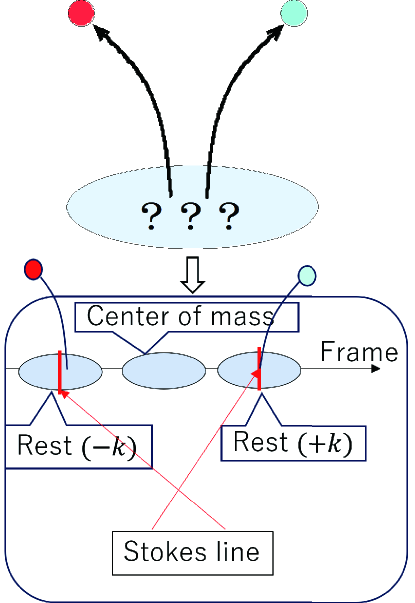
Figure 1: This figure shows the relationship between the Stokes lines and the frames when $k_{z}\neq 0$ in the center of mass frame.

We omit explicit Lorentz factors of $E$ and $\omega$ just for simplicity. Eq.(4) looks like the Schrödinger equation and can be solved as a scattering problem for the Schrödinger equation with the potential given by

$$V(t) = -q^{2}A_{z}^{2}=-q^{2}E^{2}t^{2},$$ (14)

where we set $t_{0}=0$ for simplicity. The potential is shown in Fig.2 together with the Stokes line on the complex $t$-plane.

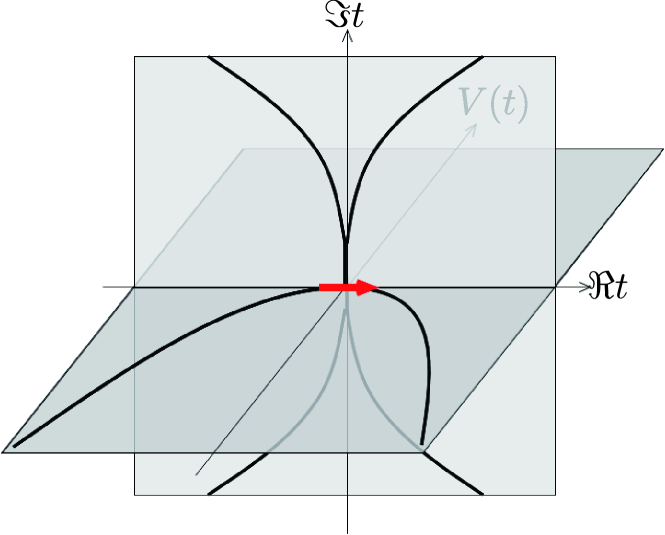
Figure 2: The potential $V(t)=-q^{2}E^{2}t^{2}$ and the Stokes lines (on the complex $t$ plane) are shown. Particle production occurs when the real $t$-axis crosses the Stokes line (indicated by the arrow at the origin).

Let us now define the vacuum not as an asymptotic state but in the tangent space at $A_{\mu}=0$. In this simplest situation, choosing $A_{\mu}=0$ gauge, one can “always” find a local vacuum attached to $A_{\mu}=0$ on which the vacuum and the Stokes line coincide. This is the very reason why particle production of the Schwinger effect can be stationary. The situation is illustrated in Fig3.

Figure 3: The potential ($V(t)=-q^{2}E^{2}t^{2}$) is illustrated on the manifold taking into account the gauge degrees of freedom. Since the Stokes phenomenon occurs on the vacuum attached to the red line (the line connecting vertices of the potential), the Stokes phenomenon is always found.

The Stokes phenomena are therefore properly defined without relying on artificial asymptotic states, and the definition of the “vacuum” is consistent with stationary radiation. The freedom of the gauge is thus properly incorpolated. The importance of the frame should be mentioned here. If the frame had not been chosen to be the rest frame of the particle, the Stokes line would not appear on the vacuum at $A_{\mu}=0$ due to the fact that $k_{z}\neq 0$. (See the definition of $\omega^{2}_{k}(t)$.) This may seem strange, but if the Stokes phenomena are considered for the centre of mass frame, the Stokes line does not appear just at the vacuum. The Stokes lines must be considered for the respective rest frames for particles and antiparticles.

We have seen that on manifolds one can always find the vacuum of particle creation which is defined locally on tangent space by choosing the section $A_{\mu}=0$ and the rest frame of the particle. So far, our calculation is fully consistent with the Schwinger’s original calculation, but after calculating the local Unruh effect we will show that we have to introduce a difference.

We have seen that the Stokes lines always coincide with the defined vacuum. For the Schwinger effect, we have seen that the local Stokes phenomenon is induced simply by the covariant derivatives. Let us now show that this is not the case with Hawking radiation and the Unruh effect. The cause of the failure tells us where the Stokes phenomenon comes from in the Unruh effect.

3 The Unruh effect and Hawking radiation

Following the Schwinger effect, one can define a local vacuum to find stationary radiation due to the Stokes phenomenon. The vacuum of the particle production is defined by choosing a frame for which the particle is at rest. In general relativity, there are two different definitions of coordinate systems in which the above condition is satisfied: the (local) Lorentz frame and the local inertial frame. Although the two frames are often considered to be physically almost identical because they give the same metric, the difference between the two frames is crucial when discussing stationary radiation on manifolds.

In order to understand the difference with gauge theory, it is first necessary to understand what happens if the derivatives are naively replaced by covariant derivatives. This manipulation gives the Klein-Gordon equation of an accelerating observer (Unruh) or on curved spacetime (Hawking), but unlike the Schwinger effect, it cannot explain the local Stokes phenomenon[35]. As already explained, the root of this problem is due to the fact that the equations of motion of the accelerating system are based on the Lorenz system and do not look at the inertial system. The only difference can appear in the vierbein, but there was no analysis of the Stokes phenomenon using this until Ref.[35]. The Bogoliubov transformation can be computed if the solution is extrapolated and analysed in the entire space, but there is a risk that extra information could be introduced by the extrapolation. We speculate that strong correlation between distant wedges is this “extra information”. We refer to this problem as the factor 2 problem.

To understand the essence of the story, it is better to consider the Unruh effect before Hawking radiation. The vacuum seen by an observer of the Unruh effect is the inertial system, not the Lorentz system. This can be confirmed by computing the vierbein. On the other hand, what the equation of motion of the accelerating observer can see is the Lorentz system (by definition). The metric is exactly the same whether it is a local inertial system or a Lorentz system, so we rarely distinguish between the two, but in the present case there must be some crucial difference. In fact, when calculating the vierbein of the Rindler spacetime given by

$$t = \frac{1+\alpha x_{r}}{\alpha}\sinh(\alpha t_{r})$$

$$x = \frac{1+\alpha x_{r}}{\alpha}\cosh(\alpha t_{r}),$$ (15)

which describes the coordinate system of an object moving at constant acceleration $\alpha$ through a flat space-time represented by $(t,x)$, one will find

$$dt = \left(1+\alpha x_{r}\right)\cosh(\alpha t_{r})dt_{r}+\sinh(\alpha t)dx_{r}$$

$$dx = \cosh(\alpha t)dx_{r}+\left(1+\alpha x_{r}\right)\sinh(\alpha t_{r})dt_{r}.$$ (16)

Obviously, the vierbein is looking at the inertial system. The metric is calculated as

$$g_{\mu\nu} = \eta_{mn}e^{m}_{\mu}e^{n}_{\nu},$$ (17)

where $\eta_{mn}$ is for the local Minkowski space. This gives the Rindler metric given by

$$ds^{2} = -(1+\alpha x_{r})^{2}dt_{r}^{2}+dx_{r}^{2}.$$ (18)

Note that the metric is identical for both (inertial and the Lorentz) frames but the explicit $t_{r}$-dependence of the vierbein appears only for the inertial system. (The vierbein of the Lorentz frame is diagonal.) As we will see, the $t_{r}$-dependence of the vierbein is where the Stokes phenomenon of stationary radiation on curved space-time comes from.

As is summarized in Ref.[1], it is possible to calculate the Bogoliubov coefficients by considering carefully the global structure of the Rindler coordinates and the relationship between the vacuum solutions written in the two coordinate systems. Let us elaborate on this (global) calculation first so that the reason for the distant correlation can be clearly understood.

We introduce the Rindler coordinates $(\tau,\xi)$ in the right wedge as

$$t = \frac{e^{\alpha\xi}}{\alpha}\sinh a\tau$$

$$z = \frac{e^{\alpha\xi}}{\alpha}\cosh a\tau,$$ (19)

where $(t,z)$ are the coordinates of the Minkowski space. Introducing the light-cone coordinate system of the Rindler space as $u=\tau-\xi,v=\tau+\xi$, we find that they are connected to the light-cone coordinate system of the Minkowski space $(U,V)$ as

$$U = -\frac{e^{-\alpha u}}{\alpha}$$

$$V = \frac{e^{\alpha v}}{\alpha}.$$ (20)

In the left wedge, we define the Rindler coordinates $(\tilde{\tau},\tilde{\xi})$.

Just for simplicity we assume massless particles and consider only the right-moving waves. In the inertial system, the field $\phi(U)$ can be expanded as

$$\phi(U) = \int^{\infty}_{0}dk\left[a_{k}f_{k}^{(M)}(U)+a_{k}^{\dagger}f_{k}^{(M)*}(U)\right],$$

$$f_{k}^{(M)}(U) = \frac{e^{-ikU}}{\sqrt{4\pi k}},$$ (21)

which defines the inertial vacuum $a_{k}|0_{M}\rangle=0$

For the right Rindler system $(\tau,\xi)$, we have

$$\phi_{R}(u) = \int^{\infty}_{0}dp\left[b_{p}^{(R)}f_{p}^{(R)}(u)+b_{p}^{(R)\dagger}f_{p}^{(R)*}(u)\right],$$

$$f_{p}^{(R)}(u) = \frac{e^{-ipu}}{\sqrt{4\pi p}}=\theta(-U)\frac{(-\alpha U)^{ip/\alpha}}{\sqrt{4\pi p}},$$ (22)

which defines the Rindler (right) vacuum $b_{p}^{(R)}|0_{R}\rangle=0$, and same calculation defines the Rindler (left) vacuum.

Although the phase space at $t=0$ can be given by $|M\rangle=|L\rangle\otimes|R\rangle$, it does not mean that the vacuum satisfies $|0_{M}\rangle=|0_{L}\rangle\otimes|0_{R}\rangle$. Indeed, using the above solutions one can find

$$|0_{M}\rangle \propto \exp\left[-\prod_{p}\left(e^{-\pi p/2\alpha}b_{p}^{L\dagger}\right)\left(e^{-\pi p/2\alpha}b_{p}^{R\dagger}\right)\right]|0_{L}\rangle\otimes|0_{R}\rangle,$$ (23)

which shows strong correlation between distant wedges. After normalization and trace about the left Rindler states, one will find the Unruh temperature $T_{U}=\hbar\alpha/2\pi ck_{B}$. What is important here is the duplication of the factor $e^{-\pi p/2\alpha}$ due to the correlation between distant wedges. This is the source of our factor 2 problem.

The global calculation “revealed” a surprising correlation of particle production between two causally disconnected wedges. More details and different approaches can be found in Ref.[1]. However, it may seem unnatural that global information is essential when its motion can be viewed as constant acceleration only over a certain period of time. Here, what we want to consider is a local system defined in the neighborhood of a point.

Let us see how the Stokes phenomenon of the Unruh effect appears locally. During the Unruh effect, an accelerating observer is looking at the inertial vacuum. Therefore the vacuum solutions of the inertial system have to be seen by an observer using the vierbein. To keep the integral of the solutions intact, we use $dt=\cosh(\alpha t_{r})dt_{r}$ to write the vacuum solutions after the Fourier transform into

$$\phi_{k}^{\pm}(t) = A_{k}e^{\pm i\int\omega dt}$$ (24)

$$= A_{k}e^{\pm i\int\omega_{k}\cosh(\alpha t_{r})dt_{r}}.$$

We are choosing the particle’s rest frame, for which ${\bf\it k}^{2}\ll\omega^{2}$. It is normally difficult to recognize the Stokes phenomenon from these solutions, but the problem can be solved using the basic properties of the EWKB. First define $Q(t)_{0}\equiv-\omega_{k}^{2}\cosh^{2}(\alpha t_{r})$ and consider the following “Schrödinger” equation

$$\left(-\frac{d^{2}}{dt^{2}}+\eta^{2}Q(t,\eta)\right)\psi(t,\eta) = 0,$$ (25)

where $\eta\gg 1$ and $Q(t,\eta)$ is expanded as

$$Q(t,\eta) = Q_{0}(t)+\eta^{-1}Q_{1}(t)+\eta^{-2}Q(t)+\cdots.$$ (26)

The solution of this equation can be written as $\psi(t,\eta)\equiv e^{\int S(t,\eta)dt}$, where $S(t,\eta)$ can be expanded as

$$S = S_{-1}(t)\eta+S_{0}(t)+S_{1}(t)\eta^{-1}+\cdots.$$ (27)

The point of this argument is that after introducing $\eta$ properly in Eq.(24), one can choose $Q_{i}(t),i\geq 1$ to find the “Schrödinger equation” which gives the solutions Eq.(24). Here $\hbar$ of quantum mechanics has been replaced by $\eta$ according to mathematical convention.

This procedure allows us to make use of a powerful analysis of the EWKB: one can calculate the Stokes lines only by using $Q_{0}(t)$. After drawing the Stokes lines, one can see that a Stokes line crosses on the real axis at the origin[35]. The Stokes lines of the Unruh effect is shown in Fig.4.

Figure 4: The Stokes lines of the Unruh effect is shown for $Q(t)=-(Cosh^{2}(2t)+0.05+0.05i)(1-0.05i)$. The degenerated Stokes lines are separated introducing small parameters.

This allowed us to expand $Q(t)_{0}$ near the origin and finally we have

$$Q(t)_{0} = -\omega_{k}^{2}\cosh(\alpha t_{r})$$ (28)

$$\simeq -\omega_{k}^{2}-\alpha^{2}\omega_{k}^{2}t_{r}^{2},$$

which gives a familiar Schrödinger equation of scattering by an inverted quadratic potential. The equation can be solved using the parabolic cylinder functions or the Weber functions, giving the MTP structure of the Stokes lines[3, 4, 35]. The Stokes phenomenon occurs at $t=0$, which can be regarded as the point of contact ($v=0$) between the observer in the accelerating system and the vacuum in the inertial system. Again, the Stokes lines coincide with the vacuum only when the vacuum is defined for the rest frame of the particles, not for the experimenter. This choice of the frame is of course consistent with other analysis[7].

The Bogoliubov coefficients of this calculation generate the Boltzmann factor $\sim e^{-\pi\omega_{k}/\alpha}$. As we have already mentioned, the global analysis of Ref.[1] gives $\sim e^{-2\pi\omega_{k}/\alpha}$, which gives the probability of strongly correlated particle production in the two distinct regions and there is the factor 2 problem. The duplication of the factor occurs due to the correlation. We can see that two particles are produced simultaneously in global analysis (which uses extrapolation) while we are calculating local and single particle production. Whether this correlation actually exists can be verified by experimentation using our results, since it appears simply in the Unruh temperature. The same applies to Hawking radiation, because Hawking radiation requires creation of a pair of negative and positive energy particles across the horizon, but only the positive energy particle outside the horizon can be observed as radiation. This is the typical “2 for 1” particle production. Two particles are produced but only one can be observed. In this case, the production probability of one particle ($P_{1}$) should be discriminated from the observation probability of one particle ($P_{1}^{obs}$). Therefore, our local analysis distinguishes “one particle production rate $P_{1}$” from “one particle observation rate $P_{1}^{obs}(=$ two particle production rate $(P_{1})^{2}$)”. There is no factor 2 problem in Hawking radiation because the “2 for 1” particle production is essential due to the conservation of the energy law.

4 Simultaneous Schwinger-Unruh-Hawking effect

Finally, it should be mentioned that the Schwinger and the Unruh effects (Hawking radiation without the event horizon because the strong electric field allows pair creation) occur simultaneously under strong electric fields. As noted above, the way to choose the vacuum for stationary particle production is “look at local inertial system, choosing rest frame for the particle and the gauge $A_{\mu}=0$”. Considering that the generated particles are accelerated by the electric field, the particles are generated from “the vacuum seen by an accelerating observer (particle)”. This is the same situation as in the case of the Unruh effect. Furthermore, unlike the Unruh effect, pair production is possible without violating the law of conservation of energy if the electric field is strong enough. Therefore, particle production is observed even in the absence of the event horizon. Furthermore, since one of the two particles of a pair does not disappear into the horizon, both are observed. As a result, this is not a “2 for 1” particle production and the Unruh temperature observed simultaneously with the Schwinger effect should show a factor of 2 difference compared to the conventional (global) Unruh effect.

Perhaps the most interesting aspect of this story is whether it is possible to verify experimentally that the Schwinger and Unruh effects occur simultaneously. As shown in this paper, the two effects arise from separate physical phenomena, and might or might not contribute in the same form. When written in the EWKB notation, it might appear that there are two contributions $Q_{0}^{Schwinger}(t)$ and $Q_{0}^{Unruh}(t)$ to $Q_{0}(t)=Q_{0}^{Schwinger}(t)+Q_{0}^{Unruh}(t)$, so that the coefficient of the inverted quadratic potential causing the Stokes phenomenon is the sum of the two contributions. One issue arises here. From the calculations so far, it is not surprising that the Schwinger and Unruh effects can occur as independent phenomena. In that case, the result should be $\beta^{tot}=\beta^{Unruh}+\beta^{Schwinger}$. Which is correct can be determined by experimental verification. The acceleration of a charged particle in a strong electromagnetic field is $\alpha=qE/m$, which, when used in “our” equation for the Unruh effect, gives an inverted quadratic potential with exactly the same coefficient as the Schwinger effect. If our considerations are correct, the actual probability of particle production should be increased, and the quantitative property is significantly different from Schwinger’s calculation. In this way, the simultaneous occurrence of the Unruh and Schwinger effects is a phenomenon that can be demonstrated experimentally. The previously mentioned problem with factor 2 of the Unruh effect can also be confirmed by experimenting. If, on the other hand, the amplification noted here did not occur, then it can be concluded that the Schwinger and Unruh effects are in fact identical physical phenomena that are linked even more deeply in the theory.

5 Conclusions and discussions

Particle production from a vacuum, including the Schwinger effect, Hawking radiation and the reheating of the universe, is a very important area of research in theoretical physics. We believe that identification of the Stokes phenomena is essential to understand these phenomena. However, conventional WKB approximation does not allow such analysis at locations where the adiabatic condition is violated. The development of the EWKB largely solved this problem, but the practice persisted for a long time, as important papers of the time set up asymptotic vacuum at a far distance. Serious problem does not arise in simple models because in such models only the physical quantity (e.g., the mass) changes with time. However, in cases where the physical quantity does not change, such as the Schwinger effect in a constant electric field, the Stokes phenomenon of the solutions raises major questions about the definition of the vacuum. This paper aims to establish the definition of the vacuum in such physical phenomena using the notion of manifolds to identify the Stokes phenomena.

The benefits of our analysis are significant: without defining a vacuum at a distance or creating a collapse gap, local stationary radiation can be analyzed using manifolds. Our results differed from the conventional calculation of the Unruh effect by a factor of 2. This factor is an indicator of whether the correlations that appear in traditional calculations are correct. This paper also discusses the possibility that the Unruh effect may alter the results of the Schwinger effect. All of these can be demonstrated by experimentation.

It is the development of the EWKB that makes it possible to deal with the seemingly complex equations that result from such analysis. By understanding the local nature of the Stokes phenomenon, one can clearly distinguish between black holes and their analogs[35, 42]. If black hole chaos[43] is due to the Stokes phenomenon[44], we hope we can get closer to the nature. We hope that our methods discussed in this paper will be useful in other areas of physics, especially in condensed matter physics.

6 Acknowledgments

The author would like to express his gratitude to Seishi Enomoto for his cooperation in the early stages of this work. In writing the revised version, we express our gratitude to Satoshi Ohya for inviting us to the seminar at Nihon University and to the participants of the seminar for clarifying points that needed to be explained.

References

- [1] N. D. Birrell and P. C. W. Davies, “Quantum Fields in Curved Space,”
- [2] L. Kofman, A. D. Linde and A. A. Starobinsky, “Towards the theory of reheating after inflation,” Phys. Rev. D 56 (1997) 3258 [hep-ph/9704452].
- [3] S. Enomoto and T. Matsuda, “The exact WKB for cosmological particle production,” JHEP 03 (2021), 090 [arXiv:2010.14835 [hep-ph]].
- [4] S. Enomoto and T. Matsuda, “The exact WKB and the Landau-Zener transition for asymmetry in cosmological particle production,” JHEP 02 (2022), 131 [arXiv:2104.02312 [hep-th]].
- [5] M. V. Berry and K. Mount, “Semiclassical approximations in wave mechanics,” Rept. Prog. Phys. 35 (1972), 315
- [6] J. S. Schwinger, “On gauge invariance and vacuum polarization,” Phys. Rev. 82 (1951), 664-679
- [7] A. Di Piazza, C. Muller, K. Z. Hatsagortsyan and C. H. Keitel, “Extremely high-intensity laser interactions with fundamental quantum systems,” Rev. Mod. Phys. 84 (2012), 1177 [arXiv:1111.3886 [hep-ph]].
- [8] J. Haro, “Topics in Quantum Field Theory in Curved Space,” [arXiv:1011.4772 [gr-qc]].
- [9] S. W. Hawking, “Particle Creation by Black Holes,” Commun. Math. Phys. 43 (1975), 199-220 [erratum: Commun. Math. Phys. 46 (1976), 206]
- [10] J. B. Hartle and S. W. Hawking, “Path Integral Derivation of Black Hole Radiance,” Phys. Rev. D 13 (1976), 2188-2203
- [11] J. S. Schwinger, “The Theory of quantized fields. 1.,” Phys. Rev. 82 (1951), 914-927
- [12] J. S. Schwinger, “The Theory of quantized fields. 2.,” Phys. Rev. 91 (1953), 713-728
- [13] J. Schwinger, “The Theory of Quantized Fields. III,” Phys. Rev. 91 (1953), 728-740
- [14] J. Schwinger, “The Theory of Quantized Fields. IV,” Phys. Rev. 92 (1953), 1283-1299
- [15] J. Schwinger, “The Theory of Quantized Fields. 5,” Phys. Rev. 93 (1954), 615-628
- [16] J. Schwinger, “The Theory of Quantized Fields. VI,” Phys. Rev. 94 (1954), 1362-1384
- [17] C. K. Dumlu and G. V. Dunne, “The Stokes Phenomenon and Schwinger Vacuum Pair Production in Time-Dependent Laser Pulses,” Phys. Rev. Lett. 104 (2010), 250402 [arXiv:1004.2509 [hep-th]].
- [18] M. E. Peskin and D. V. Schroeder, “An Introduction to Quantum Field Theory” Westview Press (1995)
- [19] “Resurgence, Physics and Numbers” edited by F. Fauvet, D. Manchon, S. Marmi and D. Sauzin, Publications of the Scuola Normale Superiore, 978-88-7642-613-1
- [20] A. Voros, “The return of the quartic oscillator – The complex WKB method”, Ann. Inst. Henri Poincare, 39 (1983), 211-338.
- [21] E. Delabaere, H. Dillinger and F. Pham: Resurgence de Voros et peeriodes des courves hyperelliptique. Annales de l’Institut Fourier, 43 (1993), 163- 199.
- [22] H. Shen and H. J. Silverstone, “Observations on the JWKB treatment of the quadratic barrier, Algebraic analysis of differential equations from microlocal analysis to exponential asymptotics”, Springer, 2008, pp. 237 - 250.
- [23] N. Honda, T. Kawai and Y. Takei, “Virtual Turning Points”, Springer (2015), ISBN 978-4-431-55702-9.
- [24] H. Taya, T. Fujimori, T. Misumi, M. Nitta and N. Sakai, “Exact WKB analysis of the vacuum pair production by time-dependent electric fields,” JHEP 03 (2021), 082 [arXiv:2010.16080 [hep-th]]
- [25] S. K. Ashok, D. P. Jatkar, R. R. John, M. Raman and J. Troost, “Exact WKB analysis of = 2 gauge theories,” JHEP 07 (2016), 115 [arXiv:1604.05520 [hep-th]]
- [26] F. Yan, “Exact WKB and the quantum Seiberg-Witten curve for 4d N = 2 pure SU(3) Yang-Mills. Abelianization,” JHEP 03 (2022), 164 [arXiv:2012.15658 [hep-th]]
- [27] A. Grassi, Q. Hao and A. Neitzke, “Exact WKB methods in SU(2) Nf = 1,” JHEP 01 (2022), 046 [arXiv:2105.03777 [hep-th]]
- [28] S. Kamata, T. Misumi, N. Sueishi and M. Ünsal, “Exact-WKB analysis for SUSY and quantum deformed potentials: Quantum mechanics with Grassmann fields and Wess-Zumino terms,” [arXiv:2111.05922 [hep-th]]
- [29] M. Alim, L. Hollands and I. Tulli, “Quantum curves, resurgence and exact WKB,” [arXiv:2203.08249 [hep-th]]
- [30] M. F. Girard, “Exact WKB-like Formulae for the Energies by means of the Quantum Hamilton-Jacobi Equation,” [arXiv:2204.02708 [quant-ph]]
- [31] A. van Spaendonck and M. Vonk, “Painlevé I and exact WKB: Stokes phenomenon for two-parameter transseries,” [arXiv:2204.09062 [hep-th]]
- [32] K. Imaizumi, “Quasi-normal modes for the D3-branes and Exact WKB analysis,” Phys. Lett. B 834 (2022), 137450 [arXiv:2207.09961 [hep-th]].
- [33] W. G. Unruh, “Notes on black hole evaporation,” Phys. Rev. D 14 (1976), 870
- [34] J. S. Bell and J. M. Leinaas, “Electrons as accelerated thermometers,” Nucl. Phys. B 212 (1983), 131
- [35] S. Enomoto and T. Matsuda, “The Exact WKB analysis and the Stokes phenomena of the Unruh effect and Hawking radiation,” JHEP 12 (2022), 037 [arXiv:2203.04501 [hep-th]].
- [36] C. K. Dumlu, “Stokes phenomenon and Hawking radiation,” Phys. Rev. D 102 (2020) no.12, 125006 [arXiv:2009.09851 [hep-th]].
- [37] O. Costin, “Asymptotics and Borel Summability” (2008), Chapman and Hall/CRC. https://doi.org/10.1201/9781420070323
- [38] V. I. Ritus, “Vacuum-vacuum amplitudes in the theory of quantum radiation by mirrors in 1+1-space and charges in 3+1-space,” Int. J. Mod. Phys. A 17 (2002), 1033-1040
- [39] V. I. Ritus, “The Symmetry, inferable from Bogoliubov transformation, between the processes induced by the mirror in two-dimensional and the charge in four-dimensional space-time,” J. Exp. Theor. Phys. 97 (2003) no.1, 10-23 [arXiv:hep-th/0309181 [hep-th]].
- [40] V. I. Ritus, “Lagrangian equations of motion of particles and photons in a Schwarzschild field,” Phys. Usp. 58 (2015) no.11, 1118-1123
- [41] G. E. Volovik, “Particle creation: Schwinger + Unruh + Hawking,” Pisma Zh. Eksp. Teor. Fiz. 116 (2022) no.9, 577-578 [arXiv:2206.02799 [gr-qc]].
- [42] S. Giovanazzi, “Hawking radiation in sonic black holes,” Phys. Rev. Lett. 94 (2005), 061302 [arXiv:physics/0411064 [physics]].
- [43] J. Maldacena, S. H. Shenker and D. Stanford, “A bound on chaos,” JHEP 08 (2016), 106 [arXiv:1503.01409 [hep-th]].
- [44] T. Morita, “Thermal Emission from Semi-classical Dynamical Systems,” Phys. Rev. Lett. 122 (2019) no.10, 101603 [arXiv:1902.06940 [hep-th]].