Low-complexity linear parameter-varying approximations of incompressible Navier-Stokes equations for truncated state-dependent Riccati feedback

Abstract

Nonlinear feedback design via state-dependent Riccati equations is well established but unfeasible for large-scale systems because of computational costs. If the system can be embedded in the class of linear parameter-varying (LPV) systems with the parameter dependency being affine-linear, then the nonlinear feedback law has a series expansion with constant and precomputable coefficients. In this work, we propose a general method to approximating nonlinear systems such that the series expansion is possible and efficient even for high-dimensional systems. We lay out the stabilization of incompressible Navier-Stokes equations as application, discuss the numerical solution of the involved matrix-valued equations, and confirm the performance of the approach in a numerical example.

1 Introduction

Nonlinear feedback design for large-scale systems is challenging, as both the complexity induced by nonlinearities and the huge computational tasks caused by the system’s size have to be resolved. The commonly used methods of backstepping [22], feedback linearization [29, Ch. 5.3], or sliding mode control [16] require structural assumptions and, thus, may not be accessible to a general computational framework. The both holistic and general approach via the Hamilton-Jacobi-Bellman (HJB) equations, however, is only feasible for very moderate system sizes or calls for model order reduction; see, e.g., [14] for a relevant discussion and an application in fluid flow control. As an alternative to reducing the system’s size, one may consider approximations to the solution of the HJB equations of lower complexity. For that, for example, truncated polynomial expansions [13] or suboptimal solutions via the so called state-dependent Riccati equation (SDRE) [2] are considered. Here, we will follow on recent developments [1] on series expansions of the SDRE approximation to the HJB solution that can mitigate the still high computational costs of repeatedly solving high-dimensional Riccati equations.

As the general setup, we consider the input-affine system

$$\dot{v}(t)=f(v(t))+Bu(t),\quad y(t)=Cv(t),$$ (1)

where for time $t>0$, $x(t)\in\mathbb{R}^{n}$ denotes the state, $u(t)\in\mathbb{R}^{p}$ and $y(t)\in\mathbb{R}^{q}$ denote the input and output, $f\colon\mathbb{R}^{n}\to\mathbb{R}^{n}$ is a possibly nonlinear function, and where $B$ and $C$ are linear input and output operators. Under the mild condition that $f$ is Lipshitz continuous and $f(0)=0$, one can factorize the nonlinearity $f(v)=A(v)v$ with a state-dependent coefficient matrix $A(v)$ and bring the system Eq. 1 into state-dependent coefficient (SDC) form:

$$\dot{v}(t)=A(v(t))v(t)+Bu(t),\quad y(t)=Cv(t);$$ (2)

see, e.g., [8, Eq. (7)]. For such systems, one can define a feedback by

$$u(t)=-B^{\mkern-1.5mu\mathsf{T}}P(v(t))v(t),$$

where $P$ solves the SDRE

$$A(v)^{\mkern-1.5mu\mathsf{T}}P+PA(v)-PBB^{\mkern-1.5mu\mathsf{T}}P=-C^{\mkern-1.5mu\mathsf{T}}C;$$ (3)

see [2] for general principles and [8] for a proof of performance beyond an asymptotic smallness condition. Because of its nonlinear and, possibly high-dimensional nature, a solve of the SDRE Eq. 3 comes at high costs that make the SDRE approach unfeasible for large systems; see [8] for an example illustrating how the effort grows with the system’s dimension.

If, however, the factorization $f(v)=A(v)v$ is affine-linear with respect to a parametrization $\rho(v)\in\mathbb{R}^{m}$ of $v$, i.e., it can be represented as

$$A(v)=A_{0}+\sum_{k=1}^{m}\rho_{k}(v)A_{k},$$ (4)

then the solution $P(v)$ of the SDRE has a first-order approximation

$$P(v)\approx P_{0}+\sum_{k=1}^{m}\rho_{k}(v)L_{k}$$

where $P_{0}$ and $L_{k}$, $k=1,\ldots,m$ can be precomputed by one Riccati and $m$ Lyapunov equations; see [1, 4]. In this work we propose a general approach for controller design that bases on approximative representations as in Eq. 4 for which we employ

• an SDC representation of the nonlinear system,

• an approximative parametrization $\hat{\rho}(v)\in\mathbb{R}^{r}$, where approximative means that $r$ is chosen small such that an exact reconstruction of $v$ from $\hat{\rho}(v)$ might not be possible, and

• an affine-linear approximation of the coefficient Eq. 4.

Also, we discuss how such an approach can be realized for flow control problems modelled by semi-discrete Navier-Stokes equations (NSE). For this, we rely on

• the coordinates provided by a proper orthogonal decomposition (POD) of the velocity states; see [24] for an introduction,

• the quadratic structure of the nonlinearity in the incompressible NSE,

• implicit treatment of the incompressibility constraint, and, importantly,

• low-rank solves for and low-rank representations of the solutions to the high-dimensional Riccati and Lyapunov equations.

We note that with this line of arguments, the feedback design by truncated SDRE approximations can be made feasible for, say, finite element approximations of general nonlinear partial differential equations (PDEs).

Apart from the proposed algorithmic advances and numerical insights into the feedback approximation, we expand here on the work of [1] insofar as the parametrization step lifts fundamental structural assumptions on the problem class. A related approach, though with updates that require the solutions of nonlinear matrix equations, can be found in [15] based on the expansion of nonlinear systems into Volterra series [27]. Furthermore, we note that, with the explicit low-complexity parametrization of the nonlinearity in an otherwise linear problem formulation, the difficulties of exponentially growing dimensions that come with tensor expansions for general nonlinearities are mitigated; see [23] for a recent discussion regarding model order reduction.

The overall procedure is explained in detail as follows. In Section 2, we explain how a low-complexity linear parameter-varying approximation can be obtained by parametrizing the state of an SDC system. The formulas for expanding the SDRE solution and state the constituting equations for the coefficients of the expansion are recalled in Section 3. Section 4 lays out how POD can be used to realize a low-complexity affine-linear parameter-varying approximation of incompressible Navier-Stokes equations and in Section 5 we briefly describe the concepts for solving the high-dimensional matrix equations. In Section 6, we provide the results of numerical experiments to show the applicability of the approach and to compare with plain static feedback. The paper is concluded in Section 7.

2 Low-complexity linear parameter-varying approximations

In this section, we consider now systems in SDC form Eq. 2. If the system state $v(t)$ is encoded into time-varying parameters $\rho(t)=\mu(v(t))\in\mathbb{R}^{m}$, with $m\leq n$, and $v(t)=\nu(\rho(t))$, where $\mu$ and $\nu$ are the corresponding encoding and decoding maps, then the SDC representation Eq. 2 can be formulated as a linear parameter-varying (LPV) system via

$$\dot{v}(t)=\widetilde{A}(\rho(t))v(t)+Bu(t),\quad y(t)=Cx(t),$$ (5)

where $\widetilde{A}(\rho):=A(\nu(\rho))$. Such an embedding of a nonlinear system into the class of LPV systems is typically called quasi LPV system; see, e.g., [21]. Here we will focus on affine-linear LPV representations, where $\widetilde{A}$ depends affine-linearly on $\rho$ so that Eq. 5 can be realized as

$$\dot{v}(t)=\left(\widetilde{A}_{0}+\sum_{k=1}^{m}\rho_{k}(t)\widetilde{A}_{k}\right)v(t)+Bu(t),\quad y(t)=Cv(t),$$

where $\rho_{k}$ is the $k$-th component of $\rho$ and where $\widetilde{A}_{0}$ and $\widetilde{A}_{k}\in\mathbb{R}^{n\times n}$ are constant, $k=1,\ldots,m$.

If the state $v$ is not exactly parametrized but only approximated with less degrees of freedom in $\hat{\rho}(t)=\hat{\mu}(v(t))\in\mathbb{R}^{r}$ such that $r\ll m$, with an inexact reconstruction

$$v(t)\approx\tilde{v}(t)=\hat{\nu}(\hat{\rho}(t))=\hat{\nu}(\hat{\mu}(v(t))),$$ (6)

then an LPV approximation of Eq. 1 is given by

$$\dot{\hat{v}}(t)=\widehat{A}(\hat{\rho}(t))\hat{v}(t)+Bu(t),\quad\hat{y}(t)=C\hat{v}(t),$$ (7)

with the approximated system matrix $\widehat{A}(\hat{\rho}):=A(\hat{\nu}(\hat{\rho}))$ and the new system state $\hat{v}(t)\in\mathbb{R}^{n}$. Note that the state $\hat{v}(t)$ is of full dimension $n$, as our reduction efforts will target the structure of the model rather than the dimension of the states. Nonetheless, the ideas and techniques of approximate low-dimensional parametrizations of states and estimates on approximation errors of standard model order reduction (MOR) schemes readily apply.

3 Series expansions of state-dependent Riccati equations

The theory of first-order approximations for a single parameter dependency by [4] has been extended in [1] to the multivariate case. We briefly recall the relevant formulas.

To prepare the argument, we assume that $v$ is parametrized through $\rho$ and consider the dependency of the SDRE solution $P$ on the current value of $\rho$, i.e., $P(\cdot)=P(\rho(\cdot))$. Then, the multivariate Taylor expansion of $P$ about $\rho_{0}=0$ up to order $K$ reads

$$P(\rho)\approx P(0)+\sum_{1\leq|\alpha|\leq K}\rho^{(\alpha)}P_{\alpha},$$ (8)

where $\alpha=(\alpha_{1},\ldots,\alpha_{m})\in\mathbb{N}^{m}$ is a multiindex with $|\alpha|:=\sum_{i=1}^{m}\alpha_{i}$, where $\rho^{(\alpha)}:=\rho_{1}^{\alpha_{1}}\rho_{2}^{\alpha_{2}}\dotsm\rho_{m}^{\alpha_{m}}$, and where, importantly, $P_{\alpha}$ are constant matrices given by

$$P_{\alpha}:=\tfrac{1}{\alpha_{1}!\alpha_{2}!\cdots\alpha_{m}!}\tfrac{\partial^{|\alpha|}}{\partial_{\rho_{1}}^{\alpha_{1}}\partial_{\rho_{2}}^{\alpha_{2}}\cdots\partial_{\rho_{m}}^{\alpha_{m}}}P(0).$$

In particular, the expansion up to order one (i.e., the associated first-order approximation) can be written as

$$P(\rho)\approx P(0)+\sum_{|\alpha|=1}\rho^{(\alpha)}P_{\alpha}=:P_{0}+\sum_{k=1}^{m}\rho_{k}L_{k}.$$ (9)

Substituting $P$ in the SDRE Eq. 3 by its series expansion Eq. 8 and considering the affine-linear dependency of $A$ on $\rho$ yields

$$\bigl{(}\sum_{k=0}^{m}\rho_{k}A_{k}\bigr{)}^{\mkern-1.5mu\mathsf{T}}\bigl{(}\sum_{|\alpha|\leq K}\rho^{(\alpha)}P_{\alpha}\bigr{)}+\bigl{(}\sum_{|\alpha|\leq K}\rho^{(\alpha)}P_{\alpha}\bigr{)}\bigl{(}\sum_{k=0}^{m}\rho_{k}A_{k}\bigr{)}$$

$$\quad{}-{}\bigl{(}\sum_{|\alpha|\leq K}\rho^{(\alpha)}P_{\alpha}\bigr{)}BB^{\mkern-1.5mu\mathsf{T}}\bigl{(}\sum_{|\alpha|\leq K}\rho^{(\alpha)}P_{\alpha}\bigr{)}=-C^{\mkern-1.5mu\mathsf{T}}C,$$

where, for compactness of the expression, we introduce $\rho_{0}=1$ and use the relevant conventions for $\alpha=0\in\mathbb{N}^{m}$.

By matching the coefficients for $\rho^{(\alpha)}$, we obtain equations for the matrices of the first-order approximation Eq. 9 as

$$A_{0}^{\mkern-1.5mu\mathsf{T}}P_{0}+P_{0}A_{0}-P_{0}BB^{\mkern-1.5mu\mathsf{T}}P_{0}=-C^{\mkern-1.5mu\mathsf{T}}C,$$ (10)

for $P_{0}$ and

$$\left(A_{0}-BB^{\mkern-1.5mu\mathsf{T}}P_{0}\right)^{\mkern-1.5mu\mathsf{T}}L_{k}+L_{k}\left(A_{0}-BB^{\mkern-1.5mu\mathsf{T}}P_{0}\right)$$

$$=-\left(A_{k}^{\mkern-1.5mu\mathsf{T}}P_{0}+P_{0}A_{k}\right)$$ (11)

for $L_{k}$, with $k=1,\ldots,m$; see also [1].

4 Approximations of Navier-Stokes equations through linear affine parametrizations

As the standard model for incompressible flows we consider spatially discretized Navier-Stokes equations (NSE). After a shift of variables that eliminates constant nonzero Dirichlet boundary conditions, the semi-discrete NSEs in the variables of the velocity $v(t)\in\mathbb{R}^{n}$ and pressure $p\in\mathbb{R}^{n_{p}}$ with control input $u$ can be written as

$$M\dot{v} =\widetilde{N}(v,v)+\widetilde{A}v+J^{\mkern-1.5mu\mathsf{T}}p+\widetilde{B}u,$$ (12a)

$$0 =Jv.$$ (12b)

At least for theoretical considerations, the incompressibility constraint Eq. 12b can be resolved and the velocity $v$ can be determined by the equivalent projected equations

$$M\dot{v}=N(v,v)+Av+Bu,$$ (13)

where $N(v,v)=\Pi^{\mkern-1.5mu\mathsf{T}}\widetilde{N}(v,v)$, where $A$ and $B$ denote $\Pi^{\mkern-1.5mu\mathsf{T}}\widetilde{A}$ and $\Pi^{\mkern-1.5mu\mathsf{T}}\widetilde{B}$, respectively, and where

$$\Pi:=I_{n}-M^{-1}J^{\mkern-1.5mu\mathsf{T}}\left(JM^{-1}J^{\mkern-1.5mu\mathsf{T}}\right)^{-1}J$$ (14)

is the so-called discrete Leray projector; see [20] for properties of $\Pi$ and formulations in the coordinates of the subspace spanned by $\Pi^{\mkern-1.5mu\mathsf{T}}$ and see [7] where we have proven that the SDRE feedback based on Eq. 13 is equivalent to that of Eq. 12.

By the homogeneity in the boundary conditions, the nonlinearity $N(v,v)$ that models the convection is linear in both arguments (see, e.g., [5] for explicit formulas of $N(\cdot,\cdot)$ in a spatial discretization) so that both

$$N_{1}(v)\colon w\mapsto N(v,w)\quad\text{and}\quad N_{2}(v)\colon w\mapsto N(w,v)$$

can be realized as state-dependent coefficient matrix and so that for any blending parameter $\lambda\in\mathbb{R}$, an SDC representation is given as

$$N(v,v)=\lambda N_{1}(v)v+(1-\lambda)N_{2}(v)v=:N_{\lambda}(v)v.$$ (15)

Even more, if in an approximative parametrization as in Eq. 6, the decoding is linear, then the induced LPV approximation is affine-linear; see [18, Rem. 2].

In fact, let $V_{r}\in\mathbb{R}^{n\times r}$ be the matrix of $r$ POD modes designed to best approximate the velocity in an $r$-dimensional subspace of $\mathbb{R}^{n}$, then with

$$\hat{\rho}(t):=V_{r}^{\mkern-1.5mu\mathsf{T}}v(t)\quad\text{and}\quad\tilde{v}(t)=V_{r}\hat{\rho}(t)$$

and the approximation property of the POD basis, we obtain

$$v(t)\approx\tilde{v}(t)=V_{r}\hat{\rho}(v(t))=\sum_{i=1}^{r}\hat{\rho}_{i}(v(t))\hat{v}_{i},$$

where $\hat{v}_{i}$, for $i=1,\dots,r$ are the columns of $V_{r}\in\mathbb{R}^{n\times r}$. By the linearity of $v\to N_{\lambda}(v)$, the SDC representation Eq. 15 is readily approximated by

$$N(v)v\approx N(\tilde{v})v=\left(\sum_{i=1}^{r}\hat{\rho}_{i}\widehat{N}_{i}\right)v$$ (16)

with $\widehat{N}_{i}:=N_{\lambda}(\hat{v}_{i})$, $i=1,\ldots,r$.

From the orthogonality of the POD basis it follows that $\tilde{v}(t)=V_{r}V_{r}^{\mkern-1.5mu\mathsf{T}}v(t)\to v(t)$ uniformly with $r\to n$, $r\leq n$, which can be translated into convergence of the LPV approximations

$$\left(\sum_{i=1}^{\hat{r}}\hat{\rho}_{i}\widehat{N}_{i}\right)\to\left(\sum_{i=1}^{r}\hat{\rho}_{i}\widehat{N}_{i}\right)\to\left(\sum_{i=1}^{n}\hat{\rho}_{i}\widehat{N}_{i}\right)=N(v),$$

for $\hat{r}\to r\to n$ and $\hat{r}\leq r\leq n$. Practically, in view of computing approximations to the SDRE solution and the associated feedback law, this means that the series expansion in Eq. 9 can be augmented or reduced by simply adding or discarding parameters and the corresponding factors $L_{k}$.

5 Numerical handling of high-dimensional matrix equations

First, we note that for systems like the spatially discretized NSEs Eq. 13, a mass matrix $M$ needs to be incorporated. Since $M$ is typically symmetric positive definite and, thus, invertible, such systems are readily transformed into the standard form of Eq. 2. In practice, however, it is beneficial to consider formulations of the Riccati and Lyapunov equations Eq. 10 and Eq. 11 without the explicit inversion:

$$A_{0}^{\mkern-1.5mu\mathsf{T}}P_{0}M+M^{\mkern-1.5mu\mathsf{T}}P_{0}A_{0}-M^{\mkern-1.5mu\mathsf{T}}P_{0}BB^{\mkern-1.5mu\mathsf{T}}P_{0}M=-C^{\mkern-1.5mu\mathsf{T}}C,$$ (17)

and

$$A_{0,\mathsf{cl}}^{\mkern-1.5mu\mathsf{T}}L_{k}M+M^{\mkern-1.5mu\mathsf{T}}L_{k}A_{0,\mathsf{cl}}=-\left(M^{\mkern-1.5mu\mathsf{T}}P_{0}A_{k}+A_{k}^{\mkern-1.5mu\mathsf{T}}P_{0}M\right),$$ (18)

for $k=1,\ldots,m$, where $A_{0,\mathsf{cl}}:=A_{0}-BB^{\mkern-1.5mu\mathsf{T}}P_{0}M$ is the closed-loop system matrix corresponding to Eq. 17; see, for example, [6]. Although, these formulations can cover also problems where the mass matrix is not invertible as they appear in differential-algebraic equations like the Navier-Stokes equations in the original formulation Eq. 12, for the presentation it is convenient to refer to the projected system Eq. 13. In practice, the system matrices in Eq. 13 and the involved projection $\Pi$ from Eq. 14 are realized only implicitly during the application of iterative matrix equation solvers for Eq. 17 and Eq. 18 like the low-rank ADI; see [9].

Another general problem occurring in the presence of high-dimensional systems is the consumption of computational resources such as time and memory. In particular, it is typically not possible to even store the large-scale dense solutions $P_{0}\in\mathbb{R}^{n\times n}$ and $L_{k}\in\mathbb{R}^{n\times n}$, $k=1,\ldots,m$. An established approach to handle this problem is the use of low-rank factorizations. The stabilizing solution of the Riccati equation Eq. 17 namely $P_{0}$ is known to be positive semi-definite such that in the case of small numbers of inputs and outputs, $p,q\ll n$, it can be well represented by a low-rank Cholesky factorization, i.e., $P_{0}\approx Z_{0}Z_{0}^{\mkern-1.5mu\mathsf{T}}$ with $Z_{0}\in\mathbb{R}^{n\times\ell_{0}}$ and $\ell_{0}\ll n$. One can find various numerical methods in the literature to efficiently compute these low-rank factors of Riccati equations without ever forming the full solution $P_{0}$; see [10] for an overview. In our numerical experiments, we rely on the low-rank Newton-Kleinman-ADI method [11].

Considering the indefinite right-hand side of Eq. 18, one needs to assume that the $L_{k}$’s are generically indefinite. Nonetheless, the low-rank factorization $P_{0}\approx Z_{0}Z_{0}^{\mkern-1.5mu\mathsf{T}}$ yields the low-rank indefinite factorization

$$M^{\mkern-1.5mu\mathsf{T}}P_{0}A_{k}+A_{k}^{\mkern-1.5mu\mathsf{T}}P_{0}M$$

$$\approx\begin{bmatrix}M^{\mkern-1.5mu\mathsf{T}}Z_{0}&A_{k}^{\mkern-1.5mu\mathsf{T}}Z_{0}\end{bmatrix}\begin{bmatrix}0&I_{\ell_{0}}\\ I_{\ell_{0}}&0\end{bmatrix}\begin{bmatrix}Z_{0}^{\mkern-1.5mu\mathsf{T}}M\\ Z_{0}^{\mkern-1.5mu\mathsf{T}}A_{k}\end{bmatrix}=C_{k}S_{k}C_{k}^{\mkern-1.5mu\mathsf{T}}.$$

Based on this factorization in the right-hand side, it is possible to similarly approximate the solution to Eq. 18 as $L_{k}\approx Z_{k}D_{k}Z_{k}^{\mkern-1.5mu\mathsf{T}}$, for $k=1,\ldots,m$, where $D_{k}$ is a symmetric but possibly indefinite matrix. Here, we are using the $LDL^{\mkern-1.5mu\mathsf{T}}$-factorized low-rank ADI method [25].

6 Numerical experiments

The code, raw data and results of the presented numerical experiments are available at [19]. For the solution of Riccati and Lyapunov equations in MATLAB 9.9.0.1467703 (R2020b), we used the solver implementations from MORLAB version 5.0 [12] and M-M.E.S.S. version 2.2 [28]. For the simulation part, we resort to our Python interface [17] between Scipy and the finite element toolbox FEniCS [26].

We consider the stabilization of the flow in the wake of a 2D cylinder through two control inlets at the periphery of the cylinder. Measurement outputs are defined as averaged velocities over a small neighborhood of three sensor points in the wake; see [5] on technical details, the detailed control setup, and on how the Dirichlet control is relaxed as penalized Robin boundary conditions.

As for the numerical setup, we consider here the Reynoldsnumber $60$ and start from the associated non-zero steady state, which is to be stabilized; see Figure 1 for the basic geometry of the example and snapshots of the steady state and periodic regime that develops if no stabilization is employed. For the spatial discretization, we use quadratic-linear Taylor-Hood finite elements on a nonuniform mesh that leads to a system of size $57\,000$. For the time integration we use an implicit-explicit Euler time stepping method that in particular treats the linear part and the incompressibility constraint implicitly, whereas the nonlinear part and the feedback is treated explicitly in time. Generally, we are concerned with a system of type Eq. 12 with $\begin{bmatrix}v(t)&p(t)\end{bmatrix}^{\mkern-1.5mu\mathsf{T}}\in\mathbb{R}^{57\,000}$ with the input $u(t)\in\mathbb{R}^{2}$ and the output $y(t)\in\mathbb{R}^{6}$ extracted from the velocity state by a linear output operator $C$ as $y(t)=Cv(t)$.

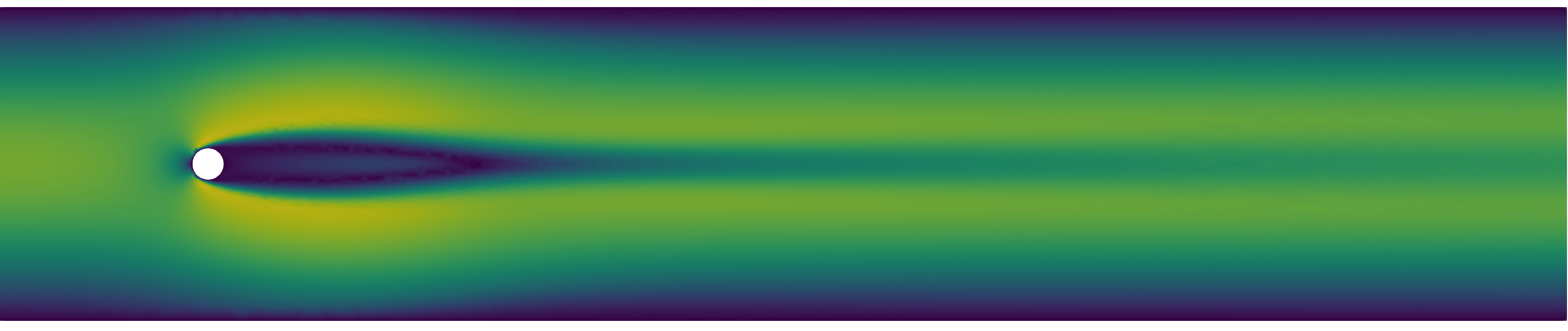
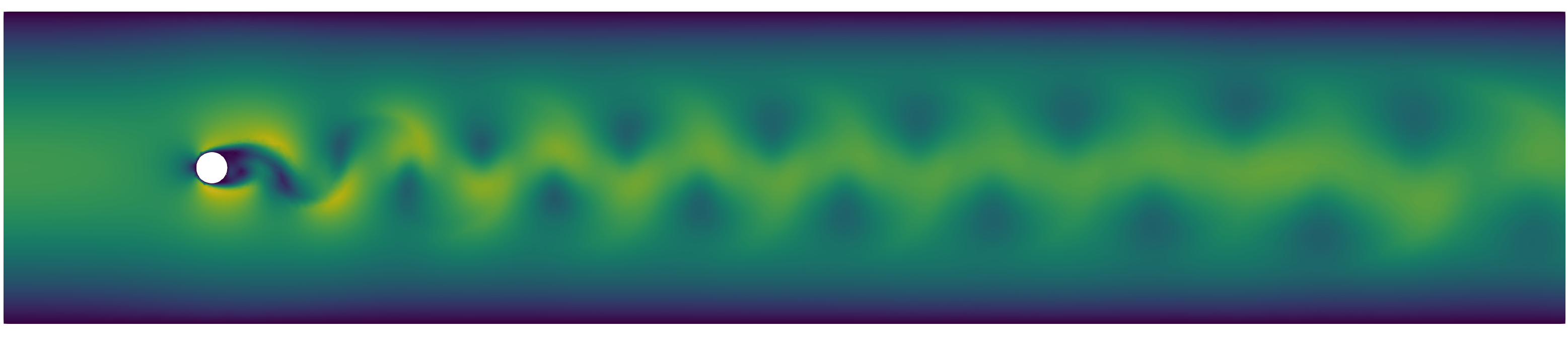
Figure 1: Snapshots of the flow in the unstable steady state and in the fully developed periodic vortex shedding regime.

The basic procedure of the simulations comprises the following steps:

• Compute the steady state for $u=0$ to be used as reference for the stabilization, for the shift of the system that removes nonzero boundary conditions, and as the starting value for the closed-loop simulations.

• Perform open-loop simulations to collect data for the POD basis for the affine-linear LPV approximation Eq. 16.

• Compute the Riccati solution $P_{0}$ and the Lyapunov solutions $L_{k}$ via Eq. 17 and Eq. 18.

• Close the loop with the nonlinear feedback law

  $$u(t)=-B^{\mkern-1.5mu\mathsf{T}}\left(P_{0}+\sum_{k=1}^{r}\hat{\rho}_{k}(v(t))L_{k}\right)Mv(t).$$ (19)

In the presented numerical study, the relevant steps were realized as follows. To acquire the data for the POD basis, we take $401$ snapshots of the velocity equally distributed on the time interval $[0,0.5]$ for the test signal

$$u(t)=\begin{bmatrix}\sin(t)&0\end{bmatrix}^{\mkern-1.5mu\mathsf{T}},$$ (20)

and define $V_{r}$ as the matrix of the $r$ leading left singular vectors with respect to the weighted inner-product induced by the mass matrix $M$ of the finite element discretization; see [3]. Then the LPV approximation Eq. 15 is computed for the NSE with $\lambda=0.75$. In the following, we denote the feedback definition by the truncated SDRE series approximation Eq. 19 of parameter dimension $r$ by xSDRE-r and the classical linear-quadratic regulator feedback, which is readily defined as $u(t)=-B^{\mkern-1.5mu\mathsf{T}}P_{0}Mv(t)$ by LQR (which is equivalent to xSDRE-0; cf. the feedback law Eq. 19).

To trigger the instabilities in the closed-loop simulations, we apply the test signal Eq. 20 on a short time $[0,t_{\mathsf{c}}]$ before we switch on the feedback at $t=t_{\mathsf{c}}$. In this way, the system will deviate from the linearization point. For $t_{\mathsf{c}}$ too large, the state may have left the region of attraction for which the linear LQR or the SDRE-based controller will stabilize the nonlinear system.

In our experiments, we employed Tikhonov regularization in the form of an $\alpha\in\{1,10^{3}\}$, which is included by replacing the original input matrix $B$ by the scaled version $\breve{B}:=\tfrac{1}{\sqrt{\alpha}}B$ in the definition of the SDRE Eq. 3 as well as in the solved Riccati and Lyapunov equations Eq. 17 and Eq. 18. Consequently, the corresponding feedback needs to be scaled as well, e.g., in the LQR case as

$$u(t)=-\frac{1}{\alpha}B^{\mkern-1.5mu\mathsf{T}}\breve{P}_{0}Mv(t),$$

where $\breve{P}_{0}$ solves the Riccati equation with $\breve{B}$. Also, we used bisection of the time domain to identify a $t_{\mathsf{c}}$ close to a critical value that marks the performance region of the controllers. For both cases of $\alpha$, we found that the xSDRE-r approach enlarges the domain of attraction of the LQR-controller. We illustrate this finding by plotting the outputs of the closed-loop systems as measured for the LQR-feedback and the xSDRE-r-feedback for various $r$. Apart from the qualitative differences in the performance, e.g., stabilization is achieved or not, in these setups, a quantitative effect of the reduction parameter $r$ as part of the nonlinear feedback definition becomes evident. In fact, for the case of $\alpha=10^{3}$ and $t_{\mathsf{c}}=0.125$, the plain LQR-feedback did not stabilize the system, while additional modes in the feedback design improved the performance steadily, until with $r=10$ stabilization was achieved; see Figure 2 with the norms of the feedback actions over time for this setup.

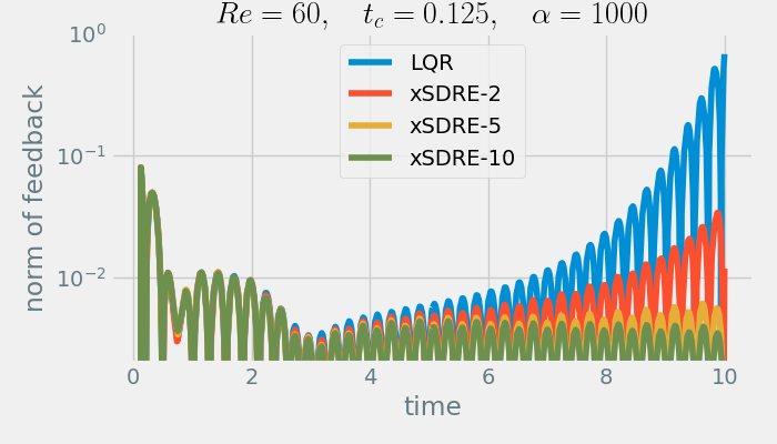
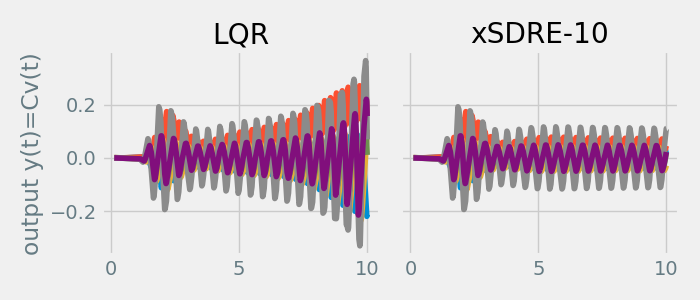
Figure 2: Norms of feedback for different $r$ and the corresponding outputs for the LQR and the xSDRE-10-feedback for the case of $\alpha=10^{3}$ and $t_{\mathsf{c}}=0.125$. A continuous performance improvement for xSDRE-r can be observed with stabilization of the system at xSDRE-10, while the classical LQR-feedback fails.

For smaller regularization parameter $\alpha=1$ that enables larger control actions, the overall region of performance is extended at the expense of a more sensitive control regime. Here, an illustrative $t_{\mathsf{c}}$ could be identified at $t=0.65$ with the LQR-feedback being not stabilizing in contrast to the xSDRE-10-feedback; see Figure 3. However, with xSDRE-2 was stabilizing while xSDRE-5 failing to do so, a clear trend for improvement in performance for larger $r$ could not be observed.

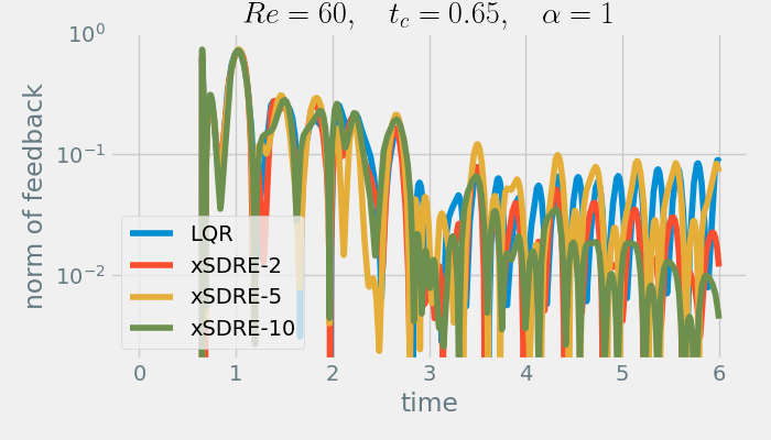
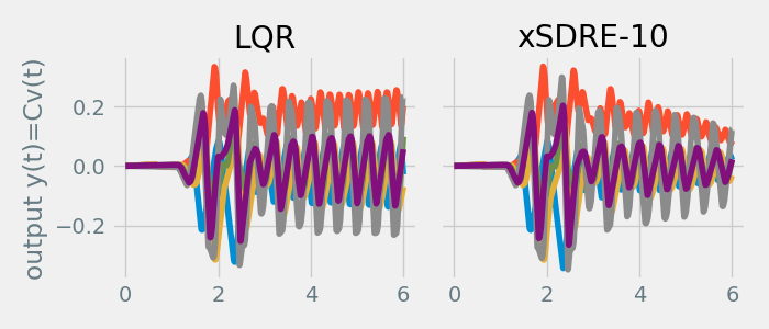
Figure 3: Norms of feedback for different $r$ and the corresponding outputs for the LQR and the xSDRE-10-feedback for the case of $\alpha=1$ and $t_{\mathsf{c}}=0.65$. The xSDRE-10-feedback is able to stabilize the system in contrast to the classical LQR approach.

Overall, we can state that the truncated SDRE approach, with an almost negligible overhead in the simulation phase, is capable to improve the feedback performance if compared to the classical LQR feedback. In particular, for larger regularization parameters the difference in the region of attraction was rather small but the smooth relation between the additional complexity $r$ and the performance turned out to be a useful hyperparameter in the feedback design. In the regime with less regularization, the xSDRE-r approach proved to give decisive advantages concerning the domain of performance at the extra cost of finding a suitable $r$.

7 Conclusion

In this work, we have presented a general framework that uses the embedding of nonlinear systems in the class of LPV systems, POD for reduction of the complexity of the parameter dimension, and the quadratic structure of the convection term in the Navier-Stokes equations to make the nonlinear feedback design through truncated expansions of the SDRE applicable. With state-of-the-art matrix equations solvers, computational feasibility of this approach was achieved too. As illustrated by a numerical example, this generic nonlinear approach provides a measurable improvement over the closely related classical LQR approach with a small additional computational effort at runtime.

Certainly, through the dependency on the POD basis for the parametrization, this approach is problem-specific. We would argue, however, that POD is a rather standard and generally applicable way to define parametrizations so that our proposed method enjoys a similarly general scope.

The potentials and needs for future work are manifold. Firstly, it would be interesting to investigate expansions of second order. Secondly, we have not paid particular attention to the definition of the coordinates for the affine LPV approximation and simply resorted to POD. Since a small dimension $r$ is most important, in particular if one wants to consider a second-order expansions of the SDRE, other, possibly nonlinear parametrizations might be considered. For the analysis of the approximation, suitable measures for the residual, e.g., in the SDRE approximation, need to be derived together with formulas for feasible evaluations in the large-scale systems case.

References

- [1] A. Alla, D. Kalise, and V. Simoncini. State-dependent Riccati equation feedback stabilization for nonlinear PDEs. Adv. Comput. Math., 49(1):9, 2023. doi:10.1007/s10444-022-09998-4.
- [2] H. T. Banks, B. M. Lewis, and H. T. Tran. Nonlinear feedback controllers and compensators: a state-dependent Riccati equation approach. Comput. Optim. Appl., 37(2):177–218, 2007. doi:10.1007/s10589-007-9015-2.
- [3] M. Baumann, P. Benner, and J. Heiland. Space-time Galerkin POD with application in optimal control of semilinear partial differential equations. SIAM J. Sci. Comput., 40(3):A1611–A1641, 2018. doi:10.1137/17M1135281.
- [4] S. C. Beeler, H. T. Tran, and H. T. Banks. Feedback control methodologies for nonlinear systems. J. Optim. Theory Appl., 107(1):1–33, 2000. doi:10.1023/A:1004607114958.
- [5] M. Behr, P. Benner, and J. Heiland. Example setups of Navier-Stokes equations with control and observation: Spatial discretization and representation via linear-quadratic matrix coefficients. e-print arXiv:1707.08711, arXiv, 2017. Mathematical Software (cs.MS). doi:10.48550/arXiv.1707.08711.
- [6] P. Benner and J. Heiland. LQG-balanced truncation low-order controller for stabilization of laminar flows. In R. King, editor, Active Flow and Combustion Control, volume 127 of Notes Numer. Fluid Mech. Multidiscip. Des., pages 365–379. Springer, Cham, 2015. doi:10.1007/978-3-319-11967-0_22.
- [7] P. Benner and J. Heiland. Nonlinear feedback stabilization of incompressible flows via updated Riccati-based gains. In 2017 IEEE 56th Annual Conference on Decision and Control (CDC), pages 1163–1168, 2017. doi:10.1109/CDC.2017.8263813.
- [8] P. Benner and J. Heiland. Exponential stability and stabilization of extended linearizations via continuous updates of Riccati-based feedback. Int. J. Robust Nonlinear Control, 28(4):1218–1232, 2018. doi:10.1002/rnc.3949.
- [9] P. Benner, J. Heiland, and S. W. R. Werner. Robust output-feedback stabilization for incompressible flows using low-dimensional -controllers. Comput. Optim. Appl., 82(1):225–249, 2022. doi:10.1007/s10589-022-00359-x.
- [10] P. Benner, J. Heiland, and S. W. R. Werner. A low-rank solution method for Riccati equations with indefinite quadratic terms. Numer. Algorithms, 92(2):1083–1103, 2023. doi:10.1007/s11075-022-01331-w.
- [11] P. Benner, M. Heinkenschloss, J. Saak, and H. K. Weichelt. Efficient solution of large-scale algebraic Riccati equations associated with index-2 DAEs via the inexact low-rank Newton-ADI method. Appl. Numer. Math., 152:338–354, 2020. doi:10.1016/j.apnum.2019.11.016.
- [12] P. Benner and S. W. R. Werner. MORLAB – Model Order Reduction LABoratory (version 5.0), August 2019. See also: https://www.mpi-magdeburg.mpg.de/projects/morlab. doi:10.5281/zenodo.3332716.
- [13] T. Breiten, K. Kunisch, and L. Pfeiffer. Infinite-horizon bilinear optimal control problems: Sensitivity analysis and polynomial feedback laws. SIAM J. Control Optim., 56(5):3184–3214, 2018. doi:10.1137/18M1173952.
- [14] T. Breiten, K. Kunisch, and L. Pfeiffer. Feedback stabilization of the two-dimensional Navier-Stokes equations by value function approximation. Appl. Math. Optim., 80(3):599–641, 2019. doi:10.1007/s00245-019-09586-x.
- [15] W. A. Cebuhar and V. Costanza. Approximation procedures for the optimal control of bilinear and nonlinear systems. J. Optim. Theory Appl., 43(4):615–627, 1984. doi:10.1007/BF00935009.
- [16] S. J. Dodds. Feedback Control: Linear, Nonlinear and Robust Techniques and Design with Industrial Applications, chapter Sliding Mode Control and Its Relatives, pages 705–792. Advanced Textbooks in Control and Signal Processing. Springer, London, 2015. doi:10.1007/978-1-4471-6675-7_10.
- [17] J. Heiland. dolfin_navier_scipy: a python Scipy FEniCS interface. Jun 2019. doi:10.5281/zenodo.3238622.
- [18] J. Heiland, P. Benner, and R. Bahmani. Convolutional neural networks for very low-dimensional LPV approximations of incompressible Navier-Stokes equations. Front. Appl. Math. Stat., 8:879140, 2022. doi:10.3389/fams.2022.879140.
- [19] J. Heiland and S. W. R. Werner. Code, data and results for numerical experiments in “Low-complexity linear parameter-varying approximations of incompressible Navier-Stokes equations for truncated state-dependent Riccati feedback” (version 1.0), March 2023. doi:10.5281/zenodo.7742469.
- [20] M. Heinkenschloss, D. C. Sorensen, and K. Sun. Balanced truncation model reduction for a class of descriptor systems with application to the Oseen equations. SIAM J. Sci. Comput., 30(2):1038–1063, 2008. doi:10.1137/070681910.
- [21] P. J. W. Koelewijn and R. Tóth. Scheduling dimension reduction of LPV models - A deep neural network approach. In 2020 American Control Conference, pages 1111–1117, 2020. doi:10.23919/ACC45564.2020.9147310.
- [22] P. V. Kokotovic. The joy of feedback: nonlinear and adaptive. IEEE Contr. Syst. Mag., 12(3):7–17, 1992. doi:10.1109/37.165507.
- [23] B. Kramer, S. Gugercin, and J. Borggaard. Nonlinear balanced truncation: Part 2 – Model reduction on manifolds. e-print 2302.02036, arXiv, 2023. Optimization and Control (math.OC). doi:10.48550/arXiv.2302.02036.
- [24] K. Kunisch and S. Volkwein. Galerkin proper orthogonal decomposition methods for a general equation in fluid dynamics. SIAM J. Numer. Anal., 40(2):492–515, 2002. doi:10.1137/S0036142900382612.
- [25] N. Lang, H. Mena, and J. Saak. An factorization based ADI algorithm for solving large-scale differential matrix equations. Proc. Appl. Math. Mech., 14(1):827–828, 2014. doi:10.1002/pamm.201410394.
- [26] A. Logg, K.-A. Mardal, and G. N. Wells. Automated Solution of Differential Equations by the Finite Element Method: The FEniCS Book, volume 84 of Lect. Notes Comput. Sci. Eng. Springer, Berlin, Heidelberg, 2012. doi:10.1007/978-3-642-23099-8.
- [27] W. J. Rugh. Nonlinear System Theory: The Volterra/Wiener Approach. The Johns Hopkins University Press, Baltimore, 1981.
- [28] J. Saak, M. Köhler, and P. Benner. M-M.E.S.S. – The Matrix Equations Sparse Solvers library (version 2.2), February 2022. See also: https://www.mpi-magdeburg.mpg.de/projects/mess. doi:10.5281/zenodo.5938237.
- [29] E. D. Sontag. Mathematical Control Theory, volume 6 of Texts in Applied Mathematics. Springer, New York, second edition, 1998. doi:10.1007/978-1-4612-0577-7.