Sketch2Saliency: Learning to Detect Salient Objects from Human Drawings

Abstract

Human sketch has already proved its worth in various visual understanding tasks (e.g., retrieval, segmentation, image-captioning, etc). In this paper, we reveal a new trait of sketches – that they are also salient. This is intuitive as sketching is a natural attentive process at its core. More specifically, we aim to study how sketches can be used as a weak label to detect salient objects present in an image. To this end, we propose a novel method that emphasises on how “salient object” could be explained by hand-drawn sketches. To accomplish this, we introduce a photo-to-sketch generation model that aims to generate sequential sketch coordinates corresponding to a given visual photo through a 2D attention mechanism. Attention maps accumulated across the time steps give rise to salient regions in the process. Extensive quantitative and qualitative experiments prove our hypothesis and delineate how our sketch-based saliency detection model gives a competitive performance compared to the state-of-the-art.

1 Introduction

As any reasonable drawing lesson would have taught you – sketching is an attentive process [26]. This paper sets out to prove just that but in the context of computer vision. In particular, we show that attention information inherently embedded in sketches can be cultivated to learn image saliency [32, 68, 89, 84].

Sketch research has flourished in the past decade, particularly with the proliferation of touchscreen devices. Much of the utilisation of sketch has anchored around its human-centric nature, in that it naturally carries personal style [56, 7], subjective abstraction [8, 55], human creativity [21], to name a few. Here we study a sketch-specific trait that has been ignored to date – sketch is also salient.

The human visual system has evolved over millions of years to develop the ability to attend [81, 24]. This attentive process is ubiquitously reflected in language (i.e., how we describe visual concepts) and art (i.e., how artists attend to different visual aspects). The vision community has also invested significant effort to model this attentive process, in the form of saliency detection [78, 84, 82, 49, 69]. The paradox facing the saliency community is however that the attention information has never been present in photos to start with – photos are mere collections of static pixels. It then comes with no surprise that most prior research has resorted to a large amount of pixel-level annotation.

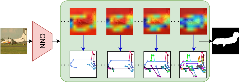
Figure 1: Sequential photo-to-sketch generation with 2D-attention to leverage sketch as a weak label for salient object detection. Aggregated 2D attention-maps till a particular instant are shown.

Although fully-supervised frameworks [36, 40, 89, 11] have been shown to produce near-perfect saliency maps, its widespread adoption is largely bottlenecked by this need for annotation. To deal with this issue, a plethora of semi/weakly-supervised methods have been introduced, which attempt to use captions [84], class-labels [46], foreground mask [68], class activation map (CAM) [71], bounding boxes [43], scribbles [87] as weak labels. We follow this push to utilise labels, but importantly introduce sketch to the mix, and show it is a competitive label modality because of the inherently embedded attentive information it possesses.

Utilising sketch as a weak label for saliency detection is nonetheless non-trivial. Sketch, primarily being abstract and sequential [24] in nature, portrays significant modality gap with photos. Therefore, we seek to build a framework that can connect sketch and photo domains via some auxiliary task. For that, we take inspiration from an actual artistic sketching process, where artists [90] attend to certain regions on an object, then render down the strokes on paper. We thus propose photo-to-sketch generation, where given a photo we aim to generate a sketch stroke-by-stroke, as an auxiliary task to bridge the two domains.

However effective in bridging the domain gap, this generation process by default does not generate pixel-wise importance values depicting a saliency map. To circumvent this problem, we make clever use of a cross-modal 2D attention module inside the sketch decoding process, which naturally predicts a local saliency map at each stroke – exactly akin to how artists refer back to the object before rendering the next stroke.

More specifically, the proposed photo-to-sketch generator is an encoder-decoder model that takes an RGB photo as input and produces a sequential sketch. The model is augmented with a 2D attention mechanism that importantly allows the model to focus on visually salient regions of the photo associated with each stroke during sketch generation. In doing so, the attention maps accumulated over the time steps of sequential sketch generation would indicate the regions on the photo that were of utmost importance. See Fig. 1 for an illustration. To further address the domain gap in supervision between pixel-wise annotation and sketch labels, we propose an additional equivariance loss to gain robustness towards perspective deformations [30] thus improving overall performance.

In our experiments we firstly report the performance of saliency maps directly predicted by the network, without convolving it with any ad hoc post-processing that is commonplace in the literature [84]. This is to spell out the true effects of using sketch for saliency detection, which is our main contribution. To further evaluate its competitiveness against other state-of-the-arts though, we also plug in our photo-to-sketch decoder in place of the image-captioning branch of a multi-source weak supervision framework that uses class-labels and text-description for saliency learning [84]. We train our network on the Sketchy dataset [58] consisting of photo-sketch pairs. It is worth noting that the training data was not intentionally collected with saliency detection in mind, rather the annotators were asked to draw a sketch that depicts the photo shown to them. This again strengthens our argument that sketch implicitly encodes saliency information which encouraged us to use it as a weak label at the first place.

In summary, our major contributions are: (a) We for the first time demonstrate the success of using sketch as a weak label in salient object detection. (b) To this end, we make clever use of sequential photo-to-sketch generation framework involving an auto-regressive decoder with 2D attention for saliency detection. (c) Comprehensive quantitative and ablative experiments delineate that our method offers significant performance gain over weakly-supervised state-of-the-arts. Moreover, this is the first work in vision community that validates the intuitive idea of “Sketch is Salient” through a simple yet effective framework.

2 Related Works

Sketch for Visual Understanding: Hand-drawn sketches, which inherit the cognitive potential of human intelligence [26], have been used in image retrieval [1, 8, 81, 12, 53, 52], generation [34, 22], editing [79], segmentation [27], image-inpainting [73], video synthesis [37], representation learning [66], 3D shape modelling [88], augmented reality [76], among others [75, 13]. Due to its commercial importance, sketch-based image retrieval (SBIR) [17, 56, 16, 80, 59, 54] has seen considerable attention within sketch-related research where the objective is to learn a sketch-photo joint-embedding space through various deep networks [8, 16, 57] for retrieving image(s) based on a sketch query. In recent times, sketches have been employed to design aesthetic pictionary-style gaming [4] and to mimic the creative angle [21] of human understanding. Growing research on the application of sketches to visual interpretation tasks establishes the representative [66] as well as discriminative [5, 14] ability of sketches to characterise the corresponding visual photo. Set upon this hypothesis, we aim to explore how saliency [36] could be explained by sparse sketches [3].

Salient Object Detection: Being pivotal to various computer vision tasks, saliency detection [69] has gained serious research attention [78, 84] as a pre-processing step in various downstream tasks. In general, recent deep learning based saliency detection frameworks can be broadly categorised into – (i) fully supervised methods [36, 40, 89, 11], and (ii) weakly/semi-supervised methods [71, 43, 84, 82]. While most fully-supervised methods make use of pixel-level semantic labels for training, different follow-up works improved the performance by modelling multi-scale features with super-pixels [36], deep hierarchical network [40] with progressive refinement, attention-guided network [89, 11]. As fully-supervised performance comes at the high cost of pixel-level labelling, various weakly-supervised methods were presented which utilise caption/tags [84, 68], bounding boxes [43], scribbles [87], centroid detection [62], CAMs [71] and foreground region masks [68] as weak labels [83]. However, unlike class-agnostic pixel-level saliency labels, image feature or category label supervisions often lack reliability [84]. Moreover, there exists added computational overhead [84, 87] while calculating such weak labels. In this work, we take a completely different idiosyncratic approach of using amateur sketches [58] as a means of weak supervision for learning image level saliency. Opposed to cumbersome architectures [84, 87], our simple framework validates and puts forth the potential of sketch as weak labels for saliency detection.

Photo to Sketch Generation: Given our hypothesis of using sketch as a label in the output space, the genre of literature that connects image (photo) in the input space with sketch in the output space is photo-to-sketch generation [41, 60, 1, 10] process. While treating photo-to-sketch generation as image-to-image translation [41] lacks the capability of modelling the stroke-by-stroke nature of human drawing, we focus on image-to-sequence generation pipeline, similar to Image Captioning [74] or Text Recognition [6], which involves a convolutional encoder followed by a RNN/LSTM decoder. Taking inspiration from the seminal work of Sketch-RNN [24], several sequential photo-to-sketch generation pipelines [60, 1, 10] have surfaced in the literature in recent times, of which [1] made use of photo-to-sketch generation for semi-supervised fine-grained SBIR. However, these prior works do not answer the question of how sequential sketch vectors could be leveraged for saliency detection, where the objective is to predict pixel-wise scalar importance value on the input image space.

Attention for Visual Understanding: Following the great success in language translation [44] under natural language processing (NLP), attention mechanism has enjoyed recognition in vision related tasks as well. Attention as a mechanism for reallocating the information according to the significance of the activation [74], plays a pivotal role in the modelling the human visual system-like behaviours. Besides incorporating the attention mechanism inside CNN architectures [29, 85], multi-head attention is now an essential building block of the transformer [64] architecture which is rapidly growing in both NLP and computer vision literature. Our attention scheme is more inclined to the design of image captioning [74] works. Moreover, we employ attention mechanism to model the saliency map inside a cross-modal photo-to-sketch generation architecture.

3 Sketch for Salient Object Detection

Overview:  To learn the saliency from sketch labels, we have access to photo-sketch pairs as $\mathcal{D}=\{(P_{i},S_{i})\}_{i}^{N}$, where every sketch corresponds to its paired photo. A few examples are shown in Fig. 2. Unlike a photo $P$ of size $\mathbb{R}^{H\times W\times 3}$, sketch holds dual-modality [3] of representation – raster and vector sequence. While in raster modality sketch can be represented as a spatial image (like a photo), the same sketch can be depicted as a sequence of coordinate points in vector modality. As raster modality lacks the stroke-by-stroke sequential hierarchical [24] information (pixels are not segmented into strokes), we use a sketch vector consisting of pen states $S=\{v_{1},v_{2},\cdots v_{T}\}$ where $T$ is the length of the sequence. Here, every point consists of a 2D absolute coordinate in a $H\times W$ canvas as $v_{i}=(x_{i},y_{i},b_{i})$, where $b_{i}\in\{0,1\}$ represents the start of a new stroke, i.e. stroke token.

In salient object detection [36], the objective is to obtain a saliency map $S_{M}$ of size $\mathbb{R}^{H\times W}$, where every scalar value $S_{M}(i,j)$ represents the importance value of that pixel belonging to the salient image region. Therefore, the research question arises as to how can we design a framework that shall learn to predict a saliency map $S_{M}$ representing the important regions of an input image, using cross-modal training data (i.e., sketch vector-photo pairs). Towards solving this, we design an image-to-sequence generation architecture consisting of a 2D attention module between a convolutional encoder and a sequential decoder.

Figure 2: Example photo-sketch pairs with original, absolute coordinate rasterised and scale normalised photos being at the top, middle and bottom respectively. It is evident that photo and sketches are not aligned even after scale normalisation, as sketch is not a pixel-wise tracing of photo edge map. This invalidates the use of classical template matching algorithms [9] for our problem.

3.1 Model Architecture

The intuition behind our architecture is that while generating every sketch coordinate at a particular time step, the attentional decoder should “look back” at the relevant region of the input photo via an attention-map, which when gathered across the whole output sketch coordinate sequence, will produce the salient regions of the input photo. Therefore, 2D spatial attention mechanism is the key that connects sequential sketch vector to spatial input photo to predict the saliency map over the input photo.

Sketch Vector Normalisation  Absolute coordinate based sketch-vector representation is scale dependent as the user can draw (see Fig. 2) the same concept in varying scales. Therefore, taking inspiration from sketch/handwriting generation literature [24], we define our sketch-coordinate in terms of offset values to make it scale-agnostic. In particular, instead of three elements with absolute coordinate ($x_{i},y_{i}$) and stroke token ($b_{i}$), now we represent every point as a five-element vector $(\Delta x_{i},\Delta y_{i},p_{i}^{1},p^{2}_{i},$ $p^{3}_{i})$, where $\Delta x_{i}=(x_{i+1}-x_{i})$ and $\Delta y_{i}=(y_{i+1}-y_{i})$. Consequently, ($p_{i}^{1},p^{2}_{i},p^{3}_{i}$) represents three pen-state situations: pen touching the paper, pen being lifted and end of drawing.

Convolutional Encoder  Instead of any complicated backbone architectures [61, 25], we use a straight-forward VGG-16 as the backbone convolutional encoder, which takes a photo (image) $P$ $\in$ $\mathbb{R}^{H\times W\times 3}$ as input and outputs multi-scale convolutional feature maps as $\mathcal{F}$ $\in$ $\{\mathcal{F}^{l},\mathcal{F}^{l-1},\mathcal{F}^{l-2}\}$, where each feature map has a spatial down-scaling factor of $\{32,16,8\}$ compared to the input spatial size with $\{512,512,256\}$ channels, respectively. This multi-scale design is in line with existing saliency detection literature [48]. $\mathcal{F}$ is later accessed by the sequential sketch decoder via an attention mechanism. Unlike multi-modal sketch-synthesis [24, 1], we purposefully ignored the variational formulation [24] as we use sketch coordinate decoding as an auxiliary task [3] to generate saliency map from sketch labels.

Sequential Decoder  Our sequential RNN decoder [24] uses the encoded feature representation of a photo $\mathcal{F}$ from convolutional encoder to predict a sequence of coordinates and pen-states, which when rasterised, would yield the sketch counterpart of the original photo. In order to model the variability towards free flow nature of sketch drawing, each off-set position $(\Delta x,\Delta y)$ is modelled using a Gaussian Mixture Model (GMM) with $M=20$ bivariate normal distributions [24] given by $p(\Delta x,\Delta y)=\sum_{j=1}^{M}\Pi_{j}\mathcal{N}(\Delta x,\Delta y|\lambda_{j})$. $\mathcal{N}(\Delta x,\Delta y|\lambda_{j})$ is the probability distribution function for a bivariate normal distribution. Each of $M$ bivariate normal distributions is parameterised by five elements $\lambda=(\mu_{x},\mu_{y},\sigma_{x},\sigma_{y},\rho_{xy})$ with mean $(\mu_{x},\mu_{y})$, standard deviation $(\sigma_{x},\sigma_{y})$ and correlation $(\rho_{xy})$. While $\mathrm{exp}$ operation is used to ensure non-negative values of mean and standard deviation, $\mathrm{tanh}$ ensures the correlation value is between $-1$ and $1$. The mixture of weights of the GMM ($\Pi\in\mathbb{R}^{M}$) is modelled by softmax normalised categorical distribution as $\sum_{j}^{M}\Pi_{j}=1$. Furthermore, three bit pen state is also modelled by a categorical distribution. Therefore, every time step’s output $y_{t}$ modelled is of size $\mathbb{R}^{5M+M+3}$, which includes $3$ logits for pen-state.

We perform a global average pooling on $\mathcal{F}^{L}$ to obtain a feature vector $f_{g}\in\mathbb{R}^{d}$ which is then fed through a linear embedding layer producing an intermediate latent vector that will be used to initialise the hidden state $h_{0}$ of decoder RNN as $h_{0}=\mathrm{tanh}(W_{k}f_{g}+b_{k})$. At a time step $t$, the update rule of the decoder network involves a recurrent function of its previous state $s_{t-1}$, and an input concatenating a context vector $g_{t}$ and coordinate vector $V_{t-1}$ (five elements) obtained in the previous time step as $s_{t}$ = $(h_{t},c_{t})$ = $RNN(s_{t-1};[g_{t},V_{t-1}])$, where $[\cdot~{};\cdot]$ denotes concatenation and start token $V_{0}$ = $(0,0,1,0,0)$. The context vector $g_{t}$ is obtained from a Multiscale 2D attention module, as described later. A fully connected layer over every time step outputs $y_{t}=W_{y}h_{t}+b_{y}$ where $y_{t}\in\mathbb{R}^{6M+3}$, which is used to sample five-element coordinate vector using GMM with bivariate normal distribution for offsets and categorical distribution for pen-states as described before.

Multi-Scale 2D Attention Module  This is the key module using which we generate the saliency map from our photo-to-sketch generation process. Compared to global average pooled fixed vector for image representation, we design a multiscale-2D attention module through which the sequential decoder looks back at a specific part of the photo at every time step of decoding which it draws. Conditioned on the current hidden state $s_{t-1}$, we first compute $s_{t-1}$-informed feature map as $\mathcal{B}^{k}_{t}=W_{M}\circledast\mathcal{F}^{k}+\hat{W}_{s}s_{t-1}$ where $k\in\{l,\;l-1,\;l-2\}$, ‘$\circledast$’ is employed with $3\times 3$ convolutional kernel $W_{M}$, and $\hat{W}_{s}$ is a learnable weight vector. Next, we combine the individual feature map via simple summation as $\mathcal{B}_{t}=\mathcal{B}^{l}_{t}+\texttt{BD}_{\times 2}(\mathcal{B}^{l-1}_{t})+\texttt{BD}_{\times 4}(\mathcal{B}^{l-2}_{t})$, and spatial size is matched using bilinear downscaling (BD) operation for $\mathcal{B}^{l-1}_{t}$ and $\mathcal{B}^{l-2}_{t}$. Thereafter, we use the multi-scale aggregated convolutional feature map $\mathcal{B}_{t}\in\mathbb{R}^{h\times w\times d}$ (with $h=\frac{H}{32},w=\frac{W}{32}$) where each spatial position in $\mathcal{B}_{t}$ represents a localised part in original input photo, to get a context vector $g_{t}$ that represents the most relevant part of $\mathcal{B}_{t}$ (later $t$ is ignored for brevity) for predicting $y_{t}$, as:

$$J=\mathrm{tanh}(W_{F}\mathcal{B}_{i,j}+W_{B}\circledast\mathcal{B}+W_{s}s_{t-1})$$

$$\alpha_{i,j}^{t}=\mathrm{softmax}(W_{a}^{T}J_{i,j})$$ (1)

$$g_{t}=\sum_{i,j}\alpha_{i,j}^{t}\cdot\mathcal{B}_{i,j}\;\;i=[1,..,h],\;j=[1,..,w]$$ (2)

where, $W_{F}$, $W_{B}$, $W_{s}$ and $W_{a}$ are learnable weights. While calculating the attention weight $\alpha_{i,j}^{t}$ at every spatial position $(i,j)$, a convolutional operation “$\circledast$” is employed with $3\times 3$ kernel $W_{B}$ to gather the neighbourhood information, as well as $1\times 1$ kernel $W_{F}$ to consider the local information. We get $\alpha^{t}\in\mathbb{R}^{h\times w}$ at every time step where every spatial position $\alpha^{t}(i,j)$ represents the importance on the input image space to draw the next coordinate point. Therefore, given maximum $T$ time steps of sequential sketch coordinate decoding, accumulating over $\alpha^{t}$ over the whole sequence gives the saliency map as follows:

$$\hat{s}_{m}(i,j)=\frac{1}{T}\sum_{i=1}^{T}\alpha^{t}(i,j)\;\rightarrow\;{s_{m}}(i,j)=\frac{\hat{s}_{m}(i,j)}{max(s_{m})}$$ (3)

where, $\hat{s}_{m}(i,j)$ is un-normalised, but gets normalised later to ensure that every positional scalar saliency value ${s_{m}}(i,j)$ lies in the range of $[0,1]$. ${s_{m}}$ is of size $h\times w$ which can be resized to input photo size $H\times W$ using bi-linear interpolation to get the final saliency map $S_{M}$.

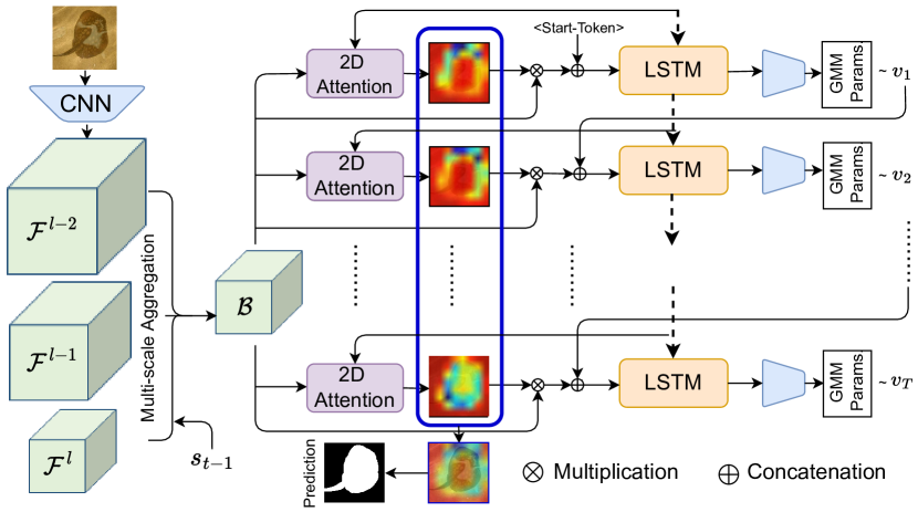
Figure 3: Illustration of photo-to-sketch generation process to learn image saliency from sketch labels. Attention maps accumulated across the time steps give rise to the saliency map.

Equivariant Regularisation  As there is a large supervision gap between pixel-level fully supervised labels [89] and weakly supervised sketch labels, we take inspiration from self-supervised learning [30] literature to bring additional inductive bias via auxiliary supervision. In particular, the assumption behind equivariant regularisation is that the output space saliency map $s_{m}$ should undergo same geometric (affine) transformations like that of input image. As the model is aware of pixel-level labelling in a fully supervised setup, the affine transformation consistency is taken care of intrinsically. However, such a protection is absent in weak supervision. There is thus a potential risk of disparity between the generated attention maps and the original photos in case of rotation, scaling or axial flips, leading to inaccurate saliency findings. To alleviate this, we introduce equivariant regularisation, ensuring that attention maps produced, are consistent with the orientation of the original image passed into the encoder network. In general, equivariant regularisation may be defined as:

$$\mathcal{R}_{\text{eqv}}=\left\|{\mathcal{X}(\mathcal{A}(P))-\mathcal{A}(\mathcal{X}(P))}\right\|_{1}$$ (4)

Here, $\mathcal{A(\cdot)}$ denotes any affine transformation applied on the image, such as axial flipping, rescaling and rotation. $\mathcal{X}(\cdot)$ denotes a encased operation to output the saliency map $S_{M}$ from input photo $P$ by accumulating attention maps across the sketch vector sequence.

3.2 Training Objective

Our photo-to-sketch generation model (Fig. 3) is trained in an end-to-end manner with three losses as follows:

Pen State Loss:  The coordinate-wise pen-state is given by $(\text{\^{p}}^{1},\text{\^{p}}^{2},\text{\^{p}}^{3})$ which is a one-hot vector and hence, optimised as a 3-class softmax classification task by using a categorical cross-entropy loss over a sequence of length $T$:

$$\mathcal{L}_{\text{coord}}=-\frac{1}{T}\sum_{t=1}^{T}\sum_{c=1}^{3}p_{t}^{c}\log{(\text{\^{p}}_{t}^{c})}$$ (5)

Stroke Loss:  The stroke loss minimises the negative log-likelihood of spatial offsets of each ground truth stroke given the predicted GMM distribution, parameterised by $(\Pi_{1},\cdots\Pi_{M})$ and $(\lambda_{1},\cdots\lambda_{M})$, at each time step $t$.

$$\mathcal{L}_{\text{stroke}}=-\frac{1}{T}\sum_{t=1}^{T}\log\big{(}\sum_{j=1}^{M}\Pi_{t,j}\mathcal{N}(\Delta x_{t},\Delta y_{t}|\lambda_{t,j})\big{)}$$ (6)

Equivariant Loss:  The equivariant regularisation loss aims to preserve spatial consistency between the input photo $P$ and the generated saliency map $S_{M}$, viz:

$$\mathcal{L}_{\text{eqv}}=\left\|{\mathcal{X}(\mathcal{A}(P))-\mathcal{A}(S_{M})}\right\|_{1}$$ (7)

Here, $\mathcal{A}$ is any affine transformation (rotation, flipping, scaling) and $\mathcal{X}(\cdot)$ denotes an encased operation to output saliency map $S_{M}$. Overall, $\mathcal{L}_{\text{sketch}}=\mathcal{L}_{\text{coord}}+\mathcal{L}_{\text{stroke}}+\mathcal{L}_{\text{eqv}}$.

4 Experiments

Datasets:  To train our saliency detection framework from sketch labels, we use Sketchy dataset [58] which contains photo-sketch pairs of $125$ classes. Each photo has at least $5$ sketches with fine-grained associations. Altogether, there are $75,471$ sketches representing $12,500$ photos. Ramer-Douglas-Peucker (RDP) algorithm [65] is applied to simplify the sketches to ease the training of LSTM based sequential decoder. Furthermore, we evaluate our model in six benchmark datasets: ECSSD [77], DUT-OMRON[78], PASCAL-S [39], PASCAL VOC2010[18], MSRA5K [42], SOD [45]. While ECSSD dataset [77] consists of 1000 natural images with numerous objects of different orientations from the web, DUT-OMRON [78] contains a total of $5168$ challenging images with one or more salient objects placed in complex backgrounds. PASCAL-S [39] incorporates a total of $850$ natural images which is the subset (validation set) of PASCAL VOC2010 [18] segmentation challenge. MSRA5K [42] holds a collection of $5,000$ natural images. SOD [45] contains 300 images, mainly created for image segmentation; [31] takes the initiative to have the pixel wise annotation of the salient objects.

Figure 4: Visualisation of raw attention-map obtained via sketch as a weak label for saliency detection. While most existing weakly supervised methods involve heuristic-based post-processing techniques [84, 43], all results shown here are directly predicted by the network without any post-processing.

Implementation Details:  Implementing our framework in PyTorch [47], we conducted experiments on a 11-GB Nvidia RTX 2080-Ti GPU. While an ImageNet pre-trained VGG-16 is used as the backbone convolutional feature extractor for input images, the sequential decoder uses a single layer LSTM with hidden state size of $512$, and embedding dimension for 2D-attention module as $256$. Maximum sequence length is set to $250$. We use Adam optimiser with learning rate $10^{-4}$ and batch size $16$ for training our model for $50$ epochs. Every image is resized to $256\times 256$ before training. We do not use any heuristic-based post-processing (e.g. CRF [87]) for evaluation. Importantly, while applying affine-transformations on input photo space for equivariant regularisation, we need to ensure that the same transformation is applied on the sketch vector labels as well.

Evaluation Metrics:  We use two evaluation metrics [84] to evaluate our method against other state-of-the-arts: (a) Mean Absolute Error (MAE) – smaller is better, and (b) maximum F-measure (max $F_{\beta}$) – larger is better, where $\beta^{2}$ is set to 0.3 [84]. Later on, we compare with recently introduced metrics [72] like weighted F-measure $(F_{\beta}^{w})$ and structural similarity measure ($S_{\alpha}$; $\alpha=0.5$).

4.1 Performance Analysis

Comparison with Alternative Label Source  In weakly supervised saliency detection, various labelling sources have been explored to help reduce cost and time of pixel-wise labelling. While [84] uses textual descriptions for saliency learning, [68] employs class-label as weak supervision, the hypothesis being that the network should have high activation at visually salient foreground regions. However, an important point to note is that most of these methods [43, 87, 62] apply heuristic-based post-processing on the initial saliency maps to get pixel-level pseudo ground-truth maps to be used by another saliency detection network during training. This dilutes the contribution of the original label source and puts more weight on the post-processing heuristic for final performance instead. For instance, while [43] leverages several iterative refinements using multi-stage training to obtain the pseudo ground-truth, scribbles [87] need an auxiliary edge-detection network for training. Constrastingly, in the first phase of our experiments, we focus on validating the un-augmented (see Fig. 4) potential of individual label sources that comes out directly after end-to-end training. Thus, among alternative label sources, we compare with class-label and text-caption, as these means allow direct usage of saliency maps from end-to-end training without any post-processing. The rest [43, 87, 62] are designed such that it is necessary to have some heuristic post-processing step. We also compare with such weakly supervised alternatives separately in Sec. 5.

Table 1 shows comparative results on ECSSD and PASCAL-S datasets. Overall, sketch has a significant edge over class-label and text-captions on both datasets. While class-label is too crude an information, text-caption contains many irrelevant details in the description such that not every word in the caption directly corresponds to salient object. In contrast, the superiority of our framework using sketch labels is attributed to two major factors – (a) Sketch inherently depicts the shape morphology of corresponding salient objects from the paired photo. (b) Our equivariant regularisation further imposes additional auxiliary supervision to learn the inductive bias via weak supervision. Although there are other weakly-supervised methods [82, 49, 87], we intentionally exclude them from Tables 1 and 2, as they need heuristic-based pre-/post-processing steps, whereas we validate the un-augmented potential of sketch for weak labels, as compared in Sec. 5.

Table 1: Evaluation (no post-processing)

Method	ECSSD		PASCAL-S
	max $F_{\beta}\uparrow$	MAE$\downarrow$	max $F_{\beta}\uparrow$	MAE$\downarrow$
Class-Label [84]	0.720	0.213	0.623	0.275
Text-Caption [84]	0.730	0.194	0.641	0.264
Sketch (Proposed)	0.781	0.152	0.705	0.228

Ablative Study:  We have conducted a thorough ablative study on ECSSD dataset to delineate the contributions of different modules present in our framework. (i) Removing sketch vector normalisation, and using absolute sketch coordinate drops the max $F_{\beta}$ value by a huge margin of $0.341$, thus signifying its utility behind achieving scale-invariance for sketch vectors. (ii) Instead of using $3\times 3$ kernel to aggregate the neighbourhood information inside the 2D attention module, using simpler 1D attention that considers convolutional feature-map as a sequence of vectors deteriorates the max $F_{\beta}$ to $0.763$ from our final value of $0.781$. (iii) Furthermore, removing equivariance loss (Eqn. 4) degrades the performance by a significant margin of $0.021$ max $F_{\beta}$ value. Therefore, it affirms that self-supervised equivariance constraints our weakly supervised model in learning invariance against a variety of perspective deformations common in wild scenarios. (iv) While learning spatial attention-based saliency from class-labels or text-caption could be attained in a single feed-forward pass, ours require sequential auto-regressive decoding, thus increasing the time complexity of our framework. Overall, it needs a CPU time of 32.3 ms to predict the saliency map of a single input image. However, the performance gain within reasonable remit of time complexity and ease of collecting amateur sketches without any expert knowledge makes sketch a potential label-alternative for saliency detection. (v) Varying number of Gaussians M in GMM from $5$ to $25$ at an interval of $5$, we get the following max $F_{\beta}$ values: $0.741$, $0.756$, $0.771$ $0.781$, and $0.779$ respectively, thus optimally choosing $M=20$. (vi) Removing multi-scale feature-map aggregation design reduce the max $F_{\beta}$ by $0.013$. (v) Overall, removing all our careful design choices and using simple spatial attention at the end of convolutional encoder as per the usual saliency literature [84] does not fully incorporate the sketching process, and an experiment sees max $F_{\beta}$ falling to $0.718$ which is even lower than that of the class/text-captions, thus validating the utility of our careful design choices.

Table 2: Linear model evaluation using fixed pre-trained features, and Semi-supervised fine-tuning from 1% and 10% labelled training data from DUTS[68] and evaluated on ECSSD [77].

Method	Conv	Linear Evaluation		Semi-supervised Evaluation
		max $F_{\beta}\uparrow$	MAE $\downarrow$	1% Train Data		10% Train Data
				max $F_{\beta}\uparrow$	MAE$\downarrow$	max $F_{\beta}\uparrow$	MAE$\downarrow$
Fully [67]	$1\times 1$	0.869	0.118	0.708	0.264	0.753	0.233
Supervised	$3\times 3$	0.872	0.111	0.713	0.251	0.761	0.224
Class [84]	$1\times 1$	0.781	0.172	0.731	0.210	0.757	0.191
Label	$3\times 3$	0.784	0.167	0.735	0.207	0.763	0.186
Text [84]	$1\times 1$	0.789	0.161	0.738	0.191	0.765	0.180
Caption	$3\times 3$	0.793	0.153	0.742	0.187	0.771	0.172
	$1\times 1$	0.832	0.129	0.788	0.148	0.817	0.145
Sketch	$3\times 3$	0.841	0.121	0.791	0.142	0.822	0.138

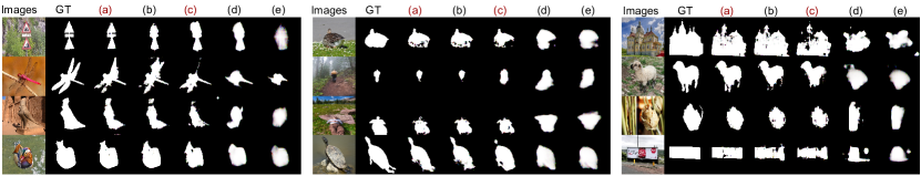
Figure 5: Qualitative results on weakly supervised saliency detection using (a) class-label + sketch (b) class-label + text-caption [84] (c) only sketch (d) only text-caption (e) only class-label. Use of sketch over text-caption significantly improves the quality of saliency map .

4.2 Photo-to-Sketch as Pre-training for Saliency

Following the self-supervised literature [33, 3], we further aim to judge the goodness of the learned convolutional feature map from our photo-to-sketch generation task for saliency detection in general. In particular, having trained the photo-to-sketch generation model from scratch, we remove the components of sequential decoder and freeze the weights of convolutional encoder, which thus acts as a standalone feature extractor. Following the linear evaluation protocol of self-supervised learning [33], we resize the last output feature map to the size of input image using bilinear interpolation, and apply one learnable layer for pixel-wise binary classification. We compare with $1\times 1$ and $3\times 3$ convolutional kernel for that learnable layer which is trained using DUTS dataset [68] containing $10,533$ training images with pixel-level labels using binary-cross entropy loss. The results in Table 2 (left) shows the primacy of sketch based weakly supervised pre-training over others, illustrating the superior generalizability of the sketch learned features over others for saliency detection. We next evaluate the semi-supervised setup, where we fine-tune the whole network [33] using smaller subsets of the training data (i.e., $1\%$ and $10\%$). Our photo-to-sketch generation using weak sketch labels as pre-training strategy augments initialisation such that even in this low data regime, our approach outperforms its supervised training counterpart under the same architecture as shown in Table 2 (right).

Table 3: Comparative study with SOTA saliency detection methods on ECSSD [77], PASCAL-S [39], MSRA5K [42], SOC [19] dataset.

Type	Method	ECSSD				PASCAL-S				MSRA5K				SOC
		max $F_{\beta}$$\uparrow$	MAE $\downarrow$	$F_{\beta}^{w}$$\uparrow$	$S_{\alpha}$$\uparrow$	max $F_{\beta}$$\uparrow$	MAE $\downarrow$	$F_{\beta}^{w}$$\uparrow$	$S_{\alpha}^{w}$$\uparrow$	max $F_{\beta}$$\uparrow$	MAE $\downarrow$	$F_{\beta}^{w}$$\uparrow$	$S_{\alpha}^{w}$$\uparrow$	max $F_{\beta}$$\uparrow$	MAE $\downarrow$	$F_{\beta}^{w}$$\uparrow$	$S_{\alpha}^{w}$$\uparrow$
FS	LEGS [67]	0.827	0.118	–	–	0.761	0.155	–	–	–	–	–	–	–	–	–	–
	DS [38]	0.882	0.122	–	–	0.763	0.176	–	–	–	–	–	–	–	–	–	–
US	BSCA [50]	0.758	0.182	–	–	0.663	0.223	–	–	0.829	0.132	–	–	–	–	–	–
	MB [86]	0.736	0.193	–	–	0.673	0.228	–	–	0.822	0.133	–	–	–	–	–	–
	MST [63]	0.724	0.155	–	–	0.657	0.194	–	–	0.809	0.980	–	–	–	–	–	–
WS	Cls-Label [68]	0.856	0.104	–	–	0.778	0.141	–	–	0.877	0.076	–	–	–	–	–	–
	Cls-Label [84]	0.773	0.162	0.721	0.753	0.736	0.176	0.672	0.734	0.836	0.094	0.812	0.842	0.581	0.167	0.521	0.657
	Text-Caption [84]	0.796	0.152	0.741	0.773	0.748	0.167	0.681	0.743	0.848	0.087	0.823	0.851	0.593	0.158	0.543	0.661
	Bounding-box [43]	0.860	0.072	0.820	0.858	–	–	–	–	–	–	–	–	–	–	–	–
	Scribble [87]	0.865	0.061	0.823	0.867	0.788	0.139	0.753	0.779	–	–	–	–	–	–	–	–
	Class-Label [49]	0.853	0.083	–	–	0.713	0.133	–	–	–	–	–	–	–	–	–	–
	Scribble [82]	0.865	0.061	0.845	0.881	0.758	0.684	0.732	0.761	–	–	–	–	–	–	–	–
	Cls+Text [84]	0.878	0.096	0.857	0.876	0.790	0.134	0.773	0.763	0.890	0.071	0.872	0.869	0.639	0.131	0.571	0.741
	Sketch	0.843	0.123	0.811	0.832	0.761	0.149	0.723	0.754	0.867	0.089	0.832	0.854	0.612	0.149	0.552	0.721
Ours	Cls-Label+Sketch	0.881	0.072	0.843	0.874	0.808	0.126	0.752	0.778	0.909	0.056	0.883	0.901	0.651	0.123	0.587	0.755

Table 4: Comparision on SOD [45] and DUT-OMRON [78].

Type	Method	SOD				DUT-OMRON
		max $F_{\beta}\uparrow$	MAE $\downarrow$	$F_{\beta}^{w}\uparrow$	$S_{\alpha}\uparrow$	max $F_{\beta}\uparrow$	MAE $\downarrow$	$F_{\beta}^{w}\uparrow$	$S_{\alpha}^{w}\uparrow$
FS	LEGS [67]	0.733	0.196	–	–	0.671	0.140	–	–
	DS [38]	0.784	0.190	–	–	0.739	0.127	–	–
US	BSCA [50]	0.656	0.252	–	–	0.613	0.196	–	–
	MB [86]	0.658	0.255	–	–	0.621	0.193	–	–
	MST [63]	0.647	0.223	–	–	0.588	0.161	–	–
WS	Cls-Label [68]	0.780	0.170	–	–	0.687	0.118	–	–
	Cls-Label [84]	0.738	0.214	0.693	0.721	0.627	0.176	0.581	0.619
	Text-Caption [84]	0.748	0.203	0.712	0.736	0.641	0.169	0.623	0.656
	Bounding-box [43]	–	–	–	–	0.680	0.081	0.650	0.770
	Scribble [87]	–	–	–	–	0.701	0.068	0.712	0.721
	Class-Label [49]	–	–	–	–	0.667	0.078	–	–
	Scribble [82]	–	–	–	–	0.758	0.069	0.745	0.754
	Cls+Text [84]	0.799	0.167	0.756	0.767	0.718	0.114	0.675	0.689
	Sketch	0.763	0.183	0.744	0.768	0.673	0.132	0.653	0.683
Ours	Cls-Label+Sketch	0.813	0.151	0.798	0.788	0.726	0.101	0.701	0.723

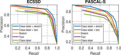
Figure 6: Precision-Recall curves of models trained from different label source under weakly supervised setup.

5 Extend Sketch Labels to MS-WSSD

Overview:  This work aims at validating the potential of sketches [26] as labels to learn visual saliency [36]. Therefore, as the primary intent of this work, we design a simple and easily reproducible sequential photo-to-sketch generation framework with an additional equivariance objective [70]. Recently, lacking a single weak supervision source, attempts have been made towards designing a Multi-Source Weakly Supervised Saliency Detection (MS-WSSD) framework [84]. Therefore, we further aim to examine the efficacy of sketches when being incorporated in such an MS-WSSD pipeline without many bells and whistles, and compare with state-of-the-art WSSD frameworks [71, 46].

We ablate the framework by Zheng et al. [84] that leveraged weak supervision via one-hot encoded class-labels and text-descriptions (captions), replacing sketch as the source of label instead of text-caption. We follow a two-stage training: First we train a classification and a photo-to-sketch generation network, which helps generate pseudo-pixel-level ground-truth saliency maps for unlabelled images. Next these pseudo-pixel-level ground-truths help train a separate saliency detection network with supervised loss.

Model: For the Classification network (C-Net), given an extracted feature-map from VGG-16 network $\mathcal{F}\in\mathbb{R}^{h\times w\times c}$, we apply $1\times 1$ convolution followed by sigmoid function to predict the coarse saliency map $s_{m}^{c}\in\mathbb{R}^{h\times w}$. Thereafter, $\mathcal{F}$ is multiplied by channel wise extended $s_{m}^{c}$ to re-weight the feature-map $\mathcal{F}^{\prime}=\mathcal{F}\cdot s_{m}^{c}$. We apply global average pooling on $\mathcal{F}^{\prime}$, followed by a linear classification layer to predict the probability distribution over classes. For the photo-to-sketch generation network (S-Net), we use our off-the-shelf network (Sec. 3). The coarse saliency map obtained by S-Net is denoted as $s_{m}^{s}\in\mathbb{R}^{h\times w}$.

Loss Functions: Firstly, we train the C-Net using available class-level training data with cross-entropy loss across class-labels and binary cross-entropy loss on $s_{m}^{c}$ with ground-truth matrix of all zeros. This acts as a regulariser to prevent the trivial saliency maps having high responses at all locations, thereby encouraging to focus on the foreground object region important for classification. We term the classification network loss as $\mathcal{L}_{\text{class}}$. Secondly, we train the S-Net model using available data with $\mathcal{L}_{\text{sketch}}$. Thirdly, we co-train C-Net and S-Net with two additional losses – attention transfer loss and attention coherence loss. Attention transfer loss aims to transfer the knowledge learned from C-Net towards S-Net, and vice-versa. The predicted coarse saliency map by C-Net (thresholded by $0.5$) acts as a ground-truth for S-Net, and vice-versa. Contrarily, the attention coherence loss utilises low-level colour similarity and super-pixels to make the predicted coarse saliency maps from C-Net and S-Net similar. Please refer to [84] for more details on the loss functions.

Post-Processing and Training Saliency Network: For the second stage of the framework, we use the predicted saliency maps from C-Net and S-Net as ground-truth for unlabelled photos to train a separate saliency detection network. Both the coarse saliency maps $s_{m}^{c}$ and $s_{m}^{s}$ are averaged and resized to that of original image using bilinear interpolation. The transformed map is processed with CRF [35] during training and binarized to form the pseudo labels, while bootstrapping loss [51] is used to train the saliency detection network (Sal-N). We use prediction from Sal-N as the final result without any post processing over there, and our results (Tables 3 and 4) follow the same.

5.1 Result Analysis

We compare our extended multi-source weakly supervised saliency detection framework, based on [84], with existing fully (FS) supervised (pixel-level label), unsupervised (US), and weakly (WS) supervised state-of-the-arts in Tables 3 and 4. Here, we additionally evaluate recently introduced metrics [72] like weighted F-measure $(F_{\beta}^{w})$ and structural similarity measure ($S_{\alpha}$; $\alpha=0.5$). Furthermore, we evaluate our sketch-based MS-WSSD framework on the recently introduced more challenging SOC [19] dataset.

Following existing weakly supervised methods [84, 68], once we train a basic network from weak labels, we use a CRF based post-processing on its predicted output to generate pseudo-ground-truths, which are then used to train a secondary saliency detection network that is finally used for evaluation. Note that our second saliency network directly predicts the saliency map without any post-processing step for faster inference. Qualitative results are shown in Fig. 5 using different sources of weak labels, and the Precision-Recall curve on ECSSD and PASCAL-S dataset in Fig. 6. Overall, we can see that sketches provide a significant edge over category-labels or text-captions and is competitive against recent complex methods like [82, 43] involving scribbles or bounding-box. In particular, adding class-labels and sketches in the MS-WSSD framework surpasses some popular supervised methods. This success of sketch as a weak saliency label also validates the fine-grained potential of sketches over text/tags in depicting visual concepts.

6 Limitations and Future Works

Despite showing how the inherently embedded attentive process in sketches can be translated to saliency maps, our approach, akin to recent sketch literature [75, 8, 22, 88], involves sketch-photo pairs that are labour-intensive to collect [28]. Removing this constraint of a strong pairing deserves immediate future work. Recent works utilising the duality of vector and raster sketches might be a good way forward [3]. Furthermore, the study of sketch-induced saliency can also be extended to scene-level, following recent push in the sketch community on scene sketches [91, 20, 15]. This could potentially reveal important insights on scene construction (e.g., what objects are most salient in a scene), and object interactions (e.g., which relationship/activity is most salient), other than just part-level saliency. As our training dataset (Sketchy) contains photo-sketch pairs mainly with a single object, the performance is limited on DUT-OMRON (Table 4) which contains multiple-objects. However, ours is still competitive (or better) compared with most weakly supervised methods [84, 68, 62]. Nevertheless, ours represents the first novel attempt to model saliency from sketches.

7 Conclusion

We have proposed a framework to generate saliency maps that utilise sketches as weak labels, circumventing the need of pixel level annotations. By introducing a sketch generation network, our model constructs saliency maps mimicking the human perception. Extensive quantitative and qualitative results prove our hypothesis – that it is indeed possible to grasp visual saliency from sketch representation of images. Our method outperforms several unsupervised and weakly-supervised state-of-the-arts, and is comparable to pixel-annotated fully-supervised methods.

Supplementary material for
Sketch2Saliency: Learning to Detect Salient Objects from Human Drawings
Ayan Kumar Bhunia¹       Subhadeep Koley^1,2       Amandeep Kumar       Aneeshan Sain^1,2
    Pinaki Nath Chowdhury^1,2      Tao Xiang^1,2     Yi-Zhe Song^1,2
1SketchX, CVSSP, University of Surrey, United Kingdom.
²iFlyTek-Surrey Joint Research Centre on Artificial Intelligence.
{a.bhunia, s.koley, a.sain, p.chowdhury, t.xiang, y.song}@surrey.ac.uk

A. Sketch Vector Normalisation

Firstly, denoting sketch-vectors as a sequence of five-element vectors with off-set values over absolute coordinate is common in sketch/handwriting literature [2, 10, 60]. It mainly models the free-flow nature of drawing via GMM [24]. Regressing to absolute coordinates otherwise, results in mean output [4] without any instance-specific variation. Secondly, offset makes sketch invariant to drawing-position in a sketch-canvas (Fig. 2). Keeping rest of the design same, replacing GMM-based loss by standard $l_{1}$ loss based absolute coordinate regression, reduces max $F_{\beta}$ value on ECSSD dataset to $0.652$ from $0.781$ (ours), thus validating the need of off-set and GMM-based design. Furthermore, sketch-vector-length varies across samples in a batch, a specific pen-state for end-of-drawing is needed to mask out loss computation from zero-appended tails of sketch-vector.

B. Multi-scale 2D Attention Module

(i) $J$ is an intermediate tensor, which is aware of three factors: (a) local and (b) neighbourhood information, of $\mathcal{B}$, and (c) previous state of auto-regressive decoder for sequential modelling. Later, $J\in\mathbb{R}^{\frac{H}{32}\times\frac{W}{32}\times d}$ helps compute the attention-map $\alpha$. (ii) $\mathcal{B}(i,j)$ signifies the $1\times 1$ convolution applied at every $(i,j)$ spatial position for local-information modelling. (iii) The first two terms are tensors of size $\mathbb{R}^{\frac{H}{32}\times\frac{W}{32}\times d}$ and $W_{s}s_{t-1}$ is a vector of size $\mathbb{R}^{d}$ which is broadcasted (standard PyTorch convention) to the required spatial size for addition. (iv) Eq. 2 is employed using $1\times 1$ convolution with kernel $W_{a}$, where softmax is applied across the spatial size, $g_{t}\in\mathbb{R}^{d}$. (v) Output of the last three max-pooling layers of VGG-16 are used for multi-scale feature aggregation which have a spatial down-scaling factor of $8,16,32$, respectively. (vi) During single-scale ablative setup, we only use the output feature-map of the last pooling layer $\mathcal{F}^{l}$.

C. Scribbles vs. Sketch

Despite taking more time, sketches hold way more structural and semantic cues than the much sparser and zero-semantics scribbles [87]. Also, temporal aspect of sketches may initiate future works on relative saliency of objects at scene level.

D. Advantage of Sequential Stroke Modelling

Firstly, as free-hand sketches are not edge-aligned with its paired photo, there is no direct way to post-process the sketch-coordinate to get aligned key-points attending the silhouettes/corners of the object. However, following [84], we design a baseline as: Apply a spatial attention module on backbone-extracted feature-map followed by global-average pooling and a fully-connected layer to directly predict the $T=100$ (fixed via RDP algorithm) absolute coordinates, assuming that the network will attend salient regions via spatial attention. Here max $F_{\beta}$ on ECSSD dataset falls to $0.692$. Importantly, we can not use off-set based representation here as by definition it relies on sequential modelling explicitly. Therefore, we adopted sequential stroke modelling with ‘look-back mechanism’ via multi-scale 2D-attention for our saliency framework.

(i) Moreover, our 1-layer LSTM based auto-regressive network is quite standard for works [2, 6, 10, 60] like image captioning, handwriting/sketch generation, text recognition, and simple to optimise. (ii) Removing pen-state prediction hurts accuracy (max $F_{\beta}$: $0.741$) as the model gets confused for large-jumps at stroke-transitions via off-set-based modelling. (iii) Furthermore, this temporal aspect of sketch may potentially convey relative saliency (sorted by stroke order) – an interesting topic for future study.

E. Correlating stroke-prediction and saliency-map quality

We used photo-to-sketch generation as an auxiliary task to solve the saliency detection problem, where performance of the latter is crucial but not the former. Moreover we found that, while avg. $F_{\beta}^{\text{max}}$ for samples whose sketch-generation metric, log-loss, (mean of Eq. 6 in nats [23] is lower (better) than $-1100$, comes to $0.824$, the same for samples with log-loss higher (worse) than $-1000$ drops to $0.736$, thus justifying the correlation quantitatively.

References

- [1] Ayan Kumar Bhunia, Pinaki Nath Chowdhury, Aneeshan Sain, Yongxin Yang, Tao Xiang, and Yi-Zhe Song. More photos are all you need: Semi-supervised learning for fine-grained sketch based image retrieval. In CVPR, 2021.
- [2] Ayan Kumar Bhunia, Pinaki Nath Chowdhury, Aneeshan Sain, Yongxin Yang, Tao Xiang, and Yi-Zhe Song. More photos are all you need: Semi-supervised learning for fine-grained sketch based image retrieval. In CVPR, 2021.
- [3] Ayan Kumar Bhunia, Pinaki Nath Chowdhury, Yongxin Yang, Timothy Hospedales, Tao Xiang, and Yi-Zhe Song. Vectorization and rasterization: Self-supervised learning for sketch and handwriting. In CVPR, 2021.
- [4] Ayan Kumar Bhunia, Ayan Das, Umar Riaz Muhammad, Yongxin Yang, Timothy M. Hospedales, Tao Xiang, Yulia Gryaditskaya, and Yi-Zhe Song. Pixelor: A competitive sketching ai agent. so you think you can beat me? In Siggraph Asia, 2020.
- [5] Ayan Kumar Bhunia, Viswanatha Reddy Gajjala, Subhadeep Koley, Rohit Kundu, Aneeshan Sain, Tao Xiang, and Yi-Zhe Song. Doodle it yourself: Class incremental learning by drawing a few sketches. In CVPR, 2022.
- [6] Ayan Kumar Bhunia, Aneeshan Sain, Amandeep Kumar, Shuvozit Ghose, Pinaki Nath Chowdhury, and Yi-Zhe Song. Joint visual semantic reasoning: Multi-stage decoder for text recognition. In ICCV, 2021.
- [7] Ayan Kumar Bhunia, Aneeshan Sain, Parth Hiren Shah, Animesh Gupta, Pinaki Nath Chowdhury, Tao Xiang, and Yi-Zhe Song. Adaptive fine-grained sketch-based image retrieval. In ECCV, 2022.
- [8] Ayan Kumar Bhunia, Yongxin Yang, Timothy M Hospedales, Tao Xiang, and Yi-Zhe Song. Sketch less for more: On-the-fly fine-grained sketch based image retrieval. In CVPR, 2020.
- [9] Roberto Brunelli. Template matching techniques in computer vision: theory and practice. John Wiley & Sons, 2009.
- [10] Nan Cao, Xin Yan, Yang Shi, and Chaoran Chen. Ai-sketcher: a deep generative model for producing high-quality sketches. In AAAI, 2019.
- [11] Shuhan Chen, Xiuli Tan, Ben Wang, and Xuelong Hu. Reverse attention for salient object detection. In ECCV, 2018.
- [12] Pinaki Nath Chowdhury, Ayan Kumar Bhunia, Viswanatha Reddy Gajjala, Aneeshan Sain, Tao Xiang, and Yi-Zhe Song. Partially does it: Towards scene-level fg-sbir with partial input. In CVPR, 2022.
- [13] Pinaki Nath Chowdhury, Ayan Kumar Bhunia, Aneeshan Sain, Subhadeep Koley, Tao Xiang, and Yi-Zhe Song. SceneTrilogy: On Human Scene-Sketch and its Complementarity with Photo and Text. In CVPR, 2023.
- [14] Pinaki Nath Chowdhury, Ayan Kumar Bhunia, Aneeshan Sain, Subhadeep Koley, Tao Xiang, and Yi-Zhe Song. What Can Human Sketches Do for Object Detection? In CVPR, 2023.
- [15] Pinaki Nath Chowdhury, Aneeshan Sain, Yulia Gryaditskaya, Ayan Kumar Bhunia, Tao Xiang, and Yi-Zhe Song. Fs-coco: Towards understanding of freehand sketches of common objects in context. In ECCV, 2022.
- [16] John Collomosse, Tu Bui, and Hailin Jin. Livesketch: Query perturbations for guided sketch-based visual search. In CVPR, 2019.
- [17] Anjan Dutta and Zeynep Akata. Semantically tied paired cycle consistency for zero-shot sketch-based image retrieval. In CVPR, 2019.
- [18] Mark Everingham, Luc Van Gool, Christopher KI Williams, John Winn, and Andrew Zisserman. The pascal visual object classes (voc) challenge. IJCV, 2010.
- [19] Deng-Ping Fan, Ming-Ming Cheng, Jiang-Jiang Liu, Shang-Hua Gao, Qibin Hou, and Ali Borji. Salient objects in clutter: Bringing salient object detection to the foreground. In ECCV, 2018.
- [20] Chengying Gao, Qi Liu, Qi Xu, Limin Wang, Jianzhuang Liu, and Changqing Zou. Sketchycoco: Image generation from freehand scene sketches. In CVPR, 2020.
- [21] Songwei Ge, Vedanuj Goswami, C Lawrence Zitnick, and Devi Parikh. Creative sketch generation. ICLR, 2020.
- [22] Arnab Ghosh, Richard Zhang, Puneet K Dokania, Oliver Wang, Alexei A Efros, Philip HS Torr, and Eli Shechtman. Interactive sketch & fill: Multiclass sketch-to-image translation. In ICCV, 2019.
- [23] Alex Graves. Generating sequences with recurrent neural networks. arXiv preprint arXiv:1308.0850, 2013.
- [24] David Ha and Douglas Eck. A neural representation of sketch drawings. ICLR, 2017.
- [25] Kaiming He, Xiangyu Zhang, Shaoqing Ren, and Jian Sun. Deep residual learning for image recognition. In CVPR, 2016.
- [26] Aaron Hertzmann. Why do line drawings work? a realism hypothesis. Perception, 2020.
- [27] Conghui Hu, Da Li, Yongxin Yang, Timothy M Hospedales, and Yi-Zhe Song. Sketch-a-segmenter: Sketch-based photo segmenter generation. IEEE TIP, 2020.
- [28] Conghui Hu, Yongxin Yang, Yunpeng Li, Timothy M Hospedales, and Yi-Zhe Song. Towards unsupervised sketch-based image retrieval. arXiv:2105.08237, 2021.
- [29] Jie Hu, Li Shen, and Gang Sun. Squeeze-and-excitation networks. In CVPR, 2018.
- [30] Wei-Chih Hung, Varun Jampani, Sifei Liu, Pavlo Molchanov, Ming-Hsuan Yang, and Jan Kautz. Scops: Self-supervised co-part segmentation. In CVPR, 2019.
- [31] Huaizu Jiang, Jingdong Wang, Zejian Yuan, Yang Wu, Nanning Zheng, and Shipeng Li. Salient object detection: A discriminative regional feature integration approach. In CVPR, 2013.
- [32] Lai Jiang, Mai Xu, Xiaofei Wang, and Leonid Sigal. Saliency-guided image translation. In CVPR, 2021.
- [33] Longlong Jing and Yingli Tian. Self-supervised visual feature learning with deep neural networks: A survey. IEEE TPAMI, 2020.
- [34] Subhadeep Koley, Ayan Kumar Bhunia, Aneeshan Sain, Pinaki Nath Chowdhury, Tao Xiang, and Yi-Zhe Song. Picture that Sketch: Photorealistic Image Generation from Abstract Sketches. In CVPR, 2023.
- [35] Philipp Krähenbühl and Vladlen Koltun. Efficient inference in fully connected crfs with gaussian edge potentials. NeurIPS, 2011.
- [36] Guanbin Li and Yizhou Yu. Visual saliency based on multiscale deep features. In CVPR, 2015.
- [37] Xiaoyu Li, Bo Zhang, Jing Liao, and Pedro Sander. Deep sketch-guided cartoon video inbetweening. IEEE TVCG, 2021.
- [38] Xi Li, Liming Zhao, Lina Wei, Ming-Hsuan Yang, Fei Wu, Yueting Zhuang, Haibin Ling, and Jingdong Wang. Deepsaliency: Multi-task deep neural network model for salient object detection. IEEE TIP, 2016.
- [39] Yin Li, Xiaodi Hou, Christof Koch, James M Rehg, and Alan L Yuille. The secrets of salient object segmentation. In CVPR, 2014.
- [40] Nian Liu and Junwei Han. Dhsnet: Deep hierarchical saliency network for salient object detection. In CVPR, 2016.
- [41] Runtao Liu, Qian Yu, and Stella X Yu. Unsupervised sketch to photo synthesis. In ECCV, 2020.
- [42] Tie Liu, Zejian Yuan, Jian Sun, Jingdong Wang, Nanning Zheng, Xiaoou Tang, and Heung-Yeung Shum. Learning to detect a salient object. IEEE TPAMI, 2010.
- [43] Yuxuan Liu, Pengjie Wang, Ying Cao, Zijian Liang, and Rynson WH Lau. Weakly-supervised salient object detection with saliency bounding boxes. IEEE TIP, 2021.
- [44] Minh-Thang Luong, Hieu Pham, and Christopher D Manning. Effective approaches to attention-based neural machine translation. EMNLP, 2015.
- [45] David Martin, Charless Fowlkes, Doron Tal, and Jitendra Malik. A database of human segmented natural images and its application to evaluating segmentation algorithms and measuring ecological statistics. In ICCV, 2001.
- [46] Seong Joon Oh, Rodrigo Benenson, Anna Khoreva, Zeynep Akata, Mario Fritz, and Bernt Schiele. Exploiting saliency for object segmentation from image level labels. In CVPR, 2017.
- [47] Adam Paszke, Sam Gross, Soumith Chintala, Gregory Chanan, Edward Yang, Zachary DeVito, Zeming Lin, Alban Desmaison, Luca Antiga, and Adam Lerer. Automatic differentiation in PyTorch. In NeurIPS Autodiff Workshop, 2017.
- [48] Yongri Piao, Wei Ji, Jingjing Li, Miao Zhang, and Huchuan Lu. Depth-induced multi-scale recurrent attention network for saliency detection. In ICCV, 2019.
- [49] Yongri Piao, Jian Wang, Miao Zhang, Zhengxuan Ma, and Huchuan Lu. To be critical: Self-calibrated weakly supervised learning for salient object detection. arXiv:2109.01770, 2021.
- [50] Yao Qin, Huchuan Lu, Yiqun Xu, and He Wang. Saliency detection via cellular automata. In CVPR, 2015.
- [51] Scott Reed, Honglak Lee, Dragomir Anguelov, Christian Szegedy, Dumitru Erhan, and Andrew Rabinovich. Training deep neural networks on noisy labels with bootstrapping. arXiv preprint arXiv:1412.6596, 2014.
- [52] Aneeshan Sain, Ayan Kumar Bhunia, Pinaki Nath Chowdhury, Aneeshan Sain, Subhadeep Koley, Tao Xiang, and Yi-Zhe Song. CLIP for All Things Zero-Shot Sketch-Based Image Retrieval, Fine-Grained or Not. In CVPR, 2023.
- [53] Aneeshan Sain, Ayan Kumar Bhunia, Subhadeep Koley, Pinaki Nath Chowdhury, Soumitri Chattopadhyay, Tao Xiang, and Yi-Zhe Song. Exploiting Unlabelled Photos for Stronger Fine-Grained SBIR. In CVPR, 2023.
- [54] Aneeshan Sain, Ayan Kumar Bhunia, Vaishnav Potlapalli, Pinaki Nath Chowdhury, Tao Xiang, and Yi-Zhe Song. Sketch3t: Test-time training for zero-shot sbir. In CVPR, 2022.
- [55] Aneeshan Sain, Ayan Kumar Bhunia, Yongxin Yang, Tao Xiang, and Yi-Zhe Song. Cross-modal hierarchical modelling for fine-grained sketch based image retrieval. In BMVC, 2020.
- [56] Aneeshan Sain, Ayan Kumar Bhunia, Yongxin Yang, Tao Xiang, and Yi-Zhe Song. Stylemeup: Towards style-agnostic sketch-based image retrieval. In CVPR, 2021.
- [57] Leo Sampaio Ferraz Ribeiro, Tu Bui, John Collomosse, and Moacir Ponti. Sketchformer: Transformer-based representation for sketched structure. In CVPR, 2020.
- [58] Patsorn Sangkloy, Nathan Burnell, Cusuh Ham, and James Hays. The sketchy database: learning to retrieve badly drawn bunnies. ACM TOG, 2016.
- [59] Yuming Shen, Li Liu, Fumin Shen, and Ling Shao. Zero-shot sketch-image hashing. In CVPR, 2018.
- [60] Jifei Song, Kaiyue Pang, Yi-Zhe Song, Tao Xiang, and Timothy M Hospedales. Learning to sketch with shortcut cycle consistency. In CVPR, 2018.
- [61] Christian Szegedy, Vincent Vanhoucke, Sergey Ioffe, Jon Shlens, and Zbigniew Wojna. Rethinking the inception architecture for computer vision. In CVPR, 2016.
- [62] Xin Tian, Ke Xu, Xin Yang, Baocai Yin, and Rynson WH Lau. Weakly-supervised salient instance detection. In BMVC, 2020.
- [63] Wei-Chih Tu, Shengfeng He, Qingxiong Yang, and Shao-Yi Chien. Real-time salient object detection with a minimum spanning tree. In CVPR, 2016.
- [64] Ashish Vaswani, Noam Shazeer, Niki Parmar, Jakob Uszkoreit, Llion Jones, Aidan N Gomez, Łukasz Kaiser, and Illia Polosukhin. Attention is all you need. In NeurIPS, 2017.
- [65] Mahes Visvalingam and J Duncan Whyatt. The douglas-peucker algorithm for line simplification: re-evaluation through visualization. In Computer Graphics Forum, 1990.
- [66] Alexander Wang, Mengye Ren, and Richard Zemel. Sketchembednet: Learning novel concepts by imitating drawings. In ICML, 2021.
- [67] Lijun Wang, Huchuan Lu, Xiang Ruan, and Ming-Hsuan Yang. Deep networks for saliency detection via local estimation and global search. In CVPR, 2015.
- [68] Lijun Wang, Huchuan Lu, Yifan Wang, Mengyang Feng, Dong Wang, Baocai Yin, and Xiang Ruan. Learning to detect salient objects with image-level supervision. In CVPR, 2017.
- [69] Wenguan Wang, Qiuxia Lai, Huazhu Fu, Jianbing Shen, Haibin Ling, and Ruigang Yang. Salient object detection in the deep learning era: An in-depth survey. IEEE T-PAMI, 2021.
- [70] Yude Wang, Jie Zhang, Meina Kan, Shiguang Shan, and Xilin Chen. Self-supervised equivariant attention mechanism for weakly supervised semantic segmentation. In CVPR, 2020.
- [71] Yunchao Wei, Jiashi Feng, Xiaodan Liang, Ming-Ming Cheng, Yao Zhao, and Shuicheng Yan. Object region mining with adversarial erasing: A simple classification to semantic segmentation approach. In CVPR, 2017.
- [72] Zhe Wu, Li Su, and Qingming Huang. Stacked cross refinement network for edge-aware salient object detection. In ICCV, 2019.
- [73] Minshan Xie, Menghan Xia, and Tien-Tsin Wong. Exploiting aliasing for manga restoration. In CVPR, 2021.
- [74] Kelvin Xu, Jimmy Ba, Ryan Kiros, Kyunghyun Cho, Aaron Courville, Ruslan Salakhudinov, Rich Zemel, and Yoshua Bengio. Show, attend and tell: Neural image caption generation with visual attention. In ICML, 2015.
- [75] Peng Xu, Timothy M Hospedales, Qiyue Yin, Yi-Zhe Song, Tao Xiang, and Liang Wang. Deep learning for free-hand sketch: A survey and a toolbox. IEEE T-PAMI, 2021.
- [76] Guowei Yan, Zhili Chen, Jimei Yang, and Huamin Wang. Interactive liquid splash modeling by user sketches. ACM TOG, 2020.
- [77] Qiong Yan, Li Xu, Jianping Shi, and Jiaya Jia. Hierarchical saliency detection. In CVPR, 2013.
- [78] Chuan Yang, Lihe Zhang, Huchuan Lu, Xiang Ruan, and Ming-Hsuan Yang. Saliency detection via graph-based manifold ranking. In CVPR, 2013.
- [79] Shuai Yang, Zhangyang Wang, Jiaying Liu, and Zongming Guo. Deep plastic surgery: Robust and controllable image editing with human-drawn sketches. In ECCV, 2020.
- [80] Sasi Kiran Yelamarthi, Shiva Krishna Reddy, Ashish Mishra, and Anurag Mittal. A zero-shot framework for sketch based image retrieval. In ECCV, 2018.
- [81] Qian Yu, Feng Liu, Yi-Zhe Song, Tao Xiang, Timothy M Hospedales, and Chen-Change Loy. Sketch me that shoe. In CVPR, 2016.
- [82] Siyue Yu, Bingfeng Zhang, Jimin Xiao, and Eng Gee Lim. Structure-consistent weakly supervised salient object detection with local saliency coherence. In AAAI, 2021.
- [83] Yu Zeng, Yunzhi Zhuge, Huchuan Lu, and Lihe Zhang. Joint learning of saliency detection and weakly supervised semantic segmentation. In CVPR, 2019.
- [84] Yu Zeng, Yunzhi Zhuge, Huchuan Lu, Lihe Zhang, Mingyang Qian, and Yizhou Yu. Multi-source weak supervision for saliency detection. In CVPR, 2019.
- [85] Han Zhang, Ian Goodfellow, Dimitris Metaxas, and Augustus Odena. Self-attention generative adversarial networks. In ICML, 2019.
- [86] Jianming Zhang, Stan Sclaroff, Zhe Lin, Xiaohui Shen, Brian Price, and Radomir Mech. Minimum barrier salient object detection at 80 fps. In ICCV, 2015.
- [87] Jing Zhang, Xin Yu, Aixuan Li, Peipei Song, Bowen Liu, and Yuchao Dai. Weakly-supervised salient object detection via scribble annotations. In CVPR, 2020.
- [88] Song-Hai Zhang, Yuan-Chen Guo, and Qing-Wen Gu. Sketch2model: View-aware 3d modeling from single free-hand sketches. In CVPR, 2021.
- [89] Xiaoning Zhang, Tiantian Wang, Jinqing Qi, Huchuan Lu, and Gang Wang. Progressive attention guided recurrent network for salient object detection. In CVPR, 2018.
- [90] Ningyuan Zheng, Yifan Jiang, and Dingjiang Huang. Strokenet: A neural painting environment. In ICLR, 2018.
- [91] Changqing Zou, Qian Yu, Ruofei Du, Haoran Mo, Yi-Zhe Song, Tao Xiang, Chengying Gao, Baoquan Chen, and Hao Zhang. Sketchyscene: Richly-annotated scene sketches. In ECCV, 2018.