Exploiting Inter-Operation Data Reuse in Scientific Applications using GOGETA 

Abstract

HPC applications are critical in various scientific domains ranging from molecular dynamics to chemistry to fluid dynamics. Conjugate Gradient (CG) is a popular application kernel used in iterative linear HPC solvers and has applications in numerous scientific domains. However, the HPCG benchmark shows that the peformance achieved by Top500 HPC systems on CG is a small fraction of the performance achieved on Linpack. While CG applications have significant portions of computations that are dense and sparse matrix multiplications, skewed SpMMs/GEMMs in the HPC solvers have poor arithmetic intensities which makes their execution highly memory bound unlike GEMMs in DNNs which have high arithmetic intensity. The problem of low intensity individual skewed GEMMs also exists in various emerging workloads from other domains like Graph Neural Networks, Transformers etc. In this work we identify various reuse opportunities between the tensors in these solver applications to extract reuse in the entire Directed Acyclic Graph of the tensor operations rather than individual tensor operations. These opportunities essentially depend on the dimensions of the tensors and the structure of the tensor dependency graph. We propose a systematic methodology to determine various kinds of reuse opportunities in the graph of operations and determine the loop order and tiling in the interdependent operations. As a result, we propose a novel mapping strategy Gogeta that improves reuse of HPC applications on spatial accelerators. We also propose a data organization strategy in the buffer. Our mapping achieves geomean 6.7x reduction in memory accesses.

1 Introduction

Sparse and Dense matrix multiplications are prime operations for a variety of applications spanning Graph Analytics [22, 13], High-Performance Computing [8, 31] and Artificial Intelligence [15, 37]. The GEMM operations used in DNNs offer vast reuse opportunities [23, 36, 28, 6] owing to their high arithmetic intensity. This has led to a plethora of spatial accelerators for DNN applications [6, 24, 19, 3] that extract reuse via customized dataflow strategies [6, 23]. Prior works have also looked at the accelerators for sparse tensor workloads [30, 14, 16, 7] which eliminate irrelevant multiplications and memory accesses.

Iterative linear solvers are key to several HPC applications ranging from chemistry to fluid dynamics. These solver applications have been slow on traditional CPUs and GPUs due to high data movement. Conjugate Gradient (CG) [17] is a popular example of an iterative linear solver. In CG, most of the operations are matrix multiplications, which intuitively should comfortably compute bound. However, for TOP500 supercomputers, the HPCG benchmark[10, 1] utilizes a fraction of compute compared to Linpack. The main reason for this is costly data movement and communication between compute clusters/pods. This is because skewed GEMMs  used in various HPC applications/kernels like CG have orders of magnitude lower arithmetic intensity compared to SpMMs/GEMMs in DNNs and offer less reuse opportunities within one operation as Fig. 5 (Sec. 3) discusses later in the paper. Thus, executing CG at the granularity of a GEMM, reading tensors from DRAM and writing the output of each GEMM to DRAM, makes it extremely memory bound leading to severe compute under-utilization.

In this work, we identify various inter-operation reuse opportunities for kernels like CG to enhance its arithmetic intensity. Our proposed inter-operation reuse is a wider generalization of traditional inter-operation pipelining, which is the idea of consuming the portion of the tensor as it is produced. This has been shown to be beneficial for accelerators for applications like Graph Neural Networks [12, 35, 25] and in Transformers [21] where the intermediate tensor is reused between a SpMM/GEMM and GEMM, reducing intermediate output data movement to and from DRAM.

Unfortunately, scientific applications introduce additional challenges that make it hard to directly apply inter-operation pipelining. They often require the output data from one operation in future tensor operations which may not be consecutive, due to which the data must remain resident in the memory hierarchy. As we discuss in detail in  Sec. 2, in CG these tensor operands have multiple downstream consumers—resulting in multiple tensor operand reuse distances that confound attempts at traditional GEMM fusion. This complex dependency graph can often complicate the optimization of loop orders and tiling strategies to determine efficient intra-operation and inter-operation dataflows.

Another challenge is that these solver applications have tensor operations with contracted rank being dominant, which does not pipeline with the next operation due to the significant number of partial sums contributing to each output element; therefore, it is not possible to simply fuse the entire CG application.  Fig. 1 shows a part of the CG graph and dependency of output of node 1 in multiple operations.

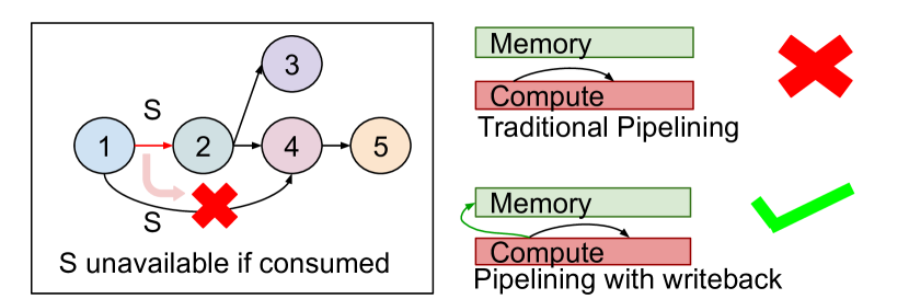
Figure 1: A part of the CG tensor dependency graph where a node represents the equation in Alg. 1 and edge represents the output of the source node equation. The data cannot be consumed and be shielded from memory hierarchy since its reused again in another tensor. Please refer to  Fig. 3 for complete graph of CG.

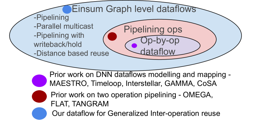
Figure 2: Our work on DAG-level dataflow covers a larger scope than works pipelining two tensor operations [21, 11, 12] and works targetting operation by operation execution [23, 36, 28, 20, 18].

Moreover, given that the graph of tensor operations becomes more complex, it is important to make sure that the loop order choice minimizes the transformation of data layouts of these tensors across various operations where that tensor is used. We use the term swizzling for the layout transformation. Thus we need to minimize swizzling.

Based on such insights from the tensor dependency graphs of various applications, we propose a systematic methodology to identify, classify and exploit reuse opportunities in an arbitrary graph of tensor operations targeting spatial accelerators. This also involves deriving the loop orders and tile sizes for individual operations since the ability to exploit the inter-operation reuse can also depend on the individual operation’s dataflow. We also propose scalable tiling strategies for applications where individual skewed GEMMs have low arithmetic intensity. Prior works on pipelining [21, 11, 12, 35] always consider the entire tensor to be local in space. However, the tiling we propose involves splitting a memory bound GEMM by the dominating rank into sub-tensors and reusing the data in a fine-grained manner between the sub-tensors.As a result of the methodology, we propose Gogeta , a new mapping strategy for arbitrary graphs of tensor operations which exploits reuse opportunities between operations. We also propose heuristics for allocating tensors inside the buffer based on tensor-level reuse distance and reuse frequency.

Our methodology is also applicable to other applications which have individual skewed GEMMs of low arithmetic intensity, including Graph Neural Networks and Transformers. However, we often refer to Conjugate Gradient as the application for demonstration purposes in this paper since its tensor dependency graph not only has the characteristics of low intensity Graph and ML workloads but also has additional unique characteristics providing opportunity to demonstrate different kinds of inter-operation reuse. Fig. 2 shows the scope of our work on inter-operation dataflows compared to prior works on accelerator dataflow.

The key contributions of this paper are:

• We introduce the challenge of skewed GEMMs/SpMMs in several HPC applications, including CG (Sec. 2).

• We identify the reuse opportunities in solver HPC applications which extend beyond the intra-operation reuse and traditional pipelining proposed by prior works (Sec. 3).

• We propose a systematic methodology to formulate the data reuse opportunities in an arbitrary DAG of tensor operations. Then we propose a systematic way of determining the loop orders and the tile sizes in order to leverage reuse from both traditional inter-operation pipelining and distance based inter-operation reuse (Sec. 4).

• We propose a scalable inter-operation tiling strategy which splits a tensor by the dominant rank and has a finer-grained inter-operation spatial communication keeping the communication in-cluster. Based on the dataflow and tiling methodology, we propose Gogeta , a mapping that reduces memory accesses and communication at the tensor dependency graph level. We also propose the notion of Tensor-operand level reuse distance for such patterns and a tensor organization strategy inside the buffer hierarchy (Sec. 5).

• Our mapping strategy Gogeta reduces the memory accesses by geomean 6.7x (range: 1.19x to 23.8x) for HPC Solver workloads.

2 Background and Related Work

2.1 Einsums, Dataflows and Mappings

Tensor operations like convolutions and matrix multiplications can be concisely and precisely expressed using Einsum (Einstein summation) notation. Einsums are well-supported state-of-the-art tools like Python’s numpy and the tensor algebra compiler TACO [4]. Compared to traditional mathematical matrix contraction notation, they have the advantage of explicitly describing the volume of data being operated on. For example, the equations below describe GEMM and CONV:

$$Z_{m,n}=\sum_{k}A_{m,k}*B_{k,n}$$ (1)

$$O_{n,h,w,k}=\sum_{c,r,s}I_{n,h+r,w+s,c}*W_{r,s,c,k}$$ (2)

In equation (1), $A$, $B$ and $Z$ are the tensors and $m$,$n$ and $k$ are dimensions/ranks. $k$ is a contracted rank and $m$ while $n$ are uncontracted ranks. For brevity the summation can be omitted as the contracted ranks do not appear in the output tensor.

Einsums can be straightforwardly implemented using loop nests, for example:

1 for m in range(M):       for m in range(M):
2  for n in range(N):       for k in range(K):
3   pfor k in range(K):      pfor n in range(N):
4    Z(m,n)+=A(m,k)*B(k,n)    Z(m,n)+=A(m,k)*B(k,n)

Dataflow refers to the loop transformations for staging the operations in compute and memory. A dataflow can affect compute utilization and the locality of tensors inside the memory hierarchy. Within the Einsum, an intra-operation dataflow is determined by the loop order and the parallelism strategy. The code sequences above represent two different loop orders: the left is $MNK$, whereas the right is $MKN$. The pfor indicates that the rank is parallelized. Thus, the left sequence is K-parallel and the right one is N-parallel. The inter-operation dataflow for multiple chained Einsums is one of the main contributions of this work, as discussed in detail in Sec. 4 and Sec. 5.

Another result of the loop order is the concept of stationarity [6]. An A-stationary dataflow signifies that $A$ is the tensor whose operands change slowest–therefore the $N$ rank is the fastest to change (as it does not index $A$). In GEMMs, there are two possible loop orders for A-stationary dataflows, $MKN$ and $KMN$. Similarly, for Output-stationary dataflows, the $K$ rank is the fastest to change, hence $MNK$ and $NMK$ are the two possible loop orders.

Tiling refers to slicing the tensors, in order for sub-tensors to fit in local memory buffers to extract reuse. Note that typically partitioning any given rank can affect multiple tensors. An example code sequence for tiling is as follows:

1 M1=M/M0; K1=K/K0; N1=N/N0
2 for m1 in range(M1):
3  for k1 in range(K1):
4   for n1 in range(N1):
5    for m0 in range(M0):
      m = m1 * M0 + m0
6     for k0 in range(K0):
       k = k1*K0+k0
7      pfor n0 in range(N0):
        n = n1*N0+n0
8       Z(m,n) += A(m,k) * B(k,n)

Note the interaction of parallelism and tiling: $N0$ is pfor in line 7. Thus in a tile, the $n0$ indices of $N$ are spatially mapped, resulting in $N1$ temporal tiles of size $N0$.

The combination of dataflow and tiling is called a mapping: a schedule of the exact execution of the workload on a specific hardware accelerator. Mapping directly affects data movement, buffer utilization, memory bandwidth utilization, and compute utilization.

2.2 HPC Applications: Chains of Einsums

Single Einsums are kernels, whereas the main loops of scientific applications consist of a chain of Einsums where tensors produced by earlier equations are consumed by later ones. This results in a tensor dependency graph dictating the high-level production/consumption of data throughout the HPC region of code. Throughout this section we use Conjugate Gradient as a running example because its tensor dependency graph exhibits multiple kinds of reuse opportunities and challenges. We briefly discuss other scientific applications with similar patterns where our work is applicable in this section.

2.2.1 Block Conjugate Gradient

Iterative linear solvers solve the system of linear equations-

$$A_{m,k}*X_{k}=B_{m}$$ (3)

While traditional conjugate gradient considers b and x as vectors, block conjugate gradient works on multiple initial guesses simultaneously for faster convergence, thus making it a matrix multiplication problem:

$$A_{m,k}*X_{k,n}=B_{m,n}$$ (4)

Input: $A_{m,m}$, $B_{m,n}$, $X_{m,n}$

$R_{m,n}=B_{m,n}-A_{m,k}*X_{k,n}$

$\Gamma_{n,n}=R_{k,n}*R{k,n}$

$P_{m,n}=R_{m,n}$

while not converged do

      1 $S_{m,n}=A_{m,k}*P_{k,n}$

      2 $\Delta_{n^{\prime},n}=P_{k,n^{\prime}}*S_{k,n}$ and $\Lambda_{n^{\prime},n}=\Delta^{-1}_{n^{\prime},j}*\Gamma_{j,n}$    // $\Delta=P^{T}S$

      3 $X_{m,n}=X_{m,n}+P_{m,j}*\Lambda_{j,n}$

      4 $R_{m,n}=R_{m,n}-S_{m,j}*\Lambda_{j,n}$

       $\Gamma\_prev_{n,n}=\Gamma_{n,n}$

      5 $\Gamma_{n^{\prime},n}=R_{k,n^{\prime}}*R_{k,n}$         // $\Gamma=R^{T}R$

       if $all(diag(\Gamma)\leq\epsilon)$ then

             break

      6$\Phi_{n^{\prime},n}=\Gamma\_{prev}^{-1}_{n^{\prime},j}*\Gamma_{j,n}$

      7 $P_{m,n}=R_{m,n}+P_{m,j}*\Phi_{j,n}$

return $X$

Algorithm 1 Chain of Einsums for Conjugate Gradient. $k$ represents contractions of size $M$ and $j$ represents contractions of size $N$ and $N^{\prime}$. Line numbers represent significant computation steps referred to throughout the text.

Alg. 1 shows the Einsums in the Conjugate Gradient Algorithm. Intuitively, we start with an initial guess $X$ and we update $R$ which at any iteration is equal to $B-AX$. If $R$ is sufficiently small, then we have reached the solution. $P$ represents the search direction for the next iteration of the loop. We have validated the functional correctness of our Einsum representation against Python’s scipy.sparse.linalg.cg.

From the perspective of tensors, $P$, $R$, $S$ and $X$ (named using English-letter variables except A) are highly skewed, for example $1000000\times 8$. In contrast, tensors like $\Delta$, $\Lambda$, $\Phi$ and $\Gamma$ (named using Greek letters) are small tensors, for example, of size $8\times 8$ Also, $A$ is the only sparse tensor in CG with a maximum shape of, for example, $1000000\times 1000000$ but with occupancy of 1-100 non-zeros per row. In Alg. 1, $M$ represents the large rank while $N$ represents the small rank. $N^{\prime}$ is equivalent to $N$ but is used to differentiate between the dimensions of square matrices in an Einsum without accidentally contracting them. As a result, line 1 is a sparse SpMM operation while all the other matrix multiplication operations are dense. The inverse operations (lines 2 and 6) are insignificant in terms of the magnitude of computation but they do affect the dependency graph since they require the complete tensor to be produced for execution. As we discuss in  Sec. 3, these matrix operations have low arithmetic intensity. The only inputs from the application side are $A$, $B$ and the initial guess, which is the initial $X$, the final output is $X$ at convergence: all other tensors are intermediates not observable by the invoking context.

Another peculiar feature about the dense matrix multiplications in Conjugate Gradient is that one matrix dimension is large. In operations denoted by lines 1, 3, 4 and 7, an uncontracted rank is the dominating rank (assuming $A$ has been compressed using a standard format like CSR). In matrix multiplication operations denoted by line 2 ($\Delta=P^{T}S$) and 5, a contracted rank is the dominating rank resulting in small outputs of the order 1$\times$1 to 16$\times$16. Contracted rank being dominating significantly diminishes the benefits of pipelining the entire CG application efficiently since most of the compute is spent in just large amounts of reduction to generate an output a usable output for the operation after it thus not exploiting the staging opportunity and affecting the overall utilization.

Fig. 3 shows the dependency graph between Einsum operations in CG. We observe that most tensor operands are not only reused in the immediate operation but also in some later operation (i.e., transitive edge) therefore having multiple reuse distances. This is unlike dependency graphs of applications like DNNs and GNNs where the output is mostly used immediately in the next operation, making fusion straightforward. One exception in Deep Learning is the skip connections in applications like ResNet.

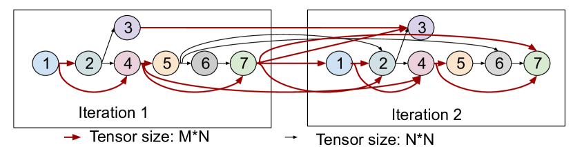
Figure 3: Tensor dependency graph of intermediates in Conjugate Gradient across first two iterations of the CG loop where a node’s number corresponds to the line in Alg. 1.

2.2.2 Other Applications with similar patterns

The pattern of variable reuse distance is commonly observed in Machine Learning models like Resnet [15] with skip connections, although ResNet has a high arithmetic intensity per Einsum. Its also observed in other solver methods like GMRES [32] and BiCGStab [34]. The problem of low arithmetic intensity individual skewed GEMMs is common in workloads like Graph Neural Networks [22].

For example, a layer of GCN (Graph Convolution Network) has the following Einsums (Only A is sparse).

Variables: $A_{m,m},~{}~{}X0_{m,n},~{}~{}Z_{m,n},~{}~{}W_{n,o},~{}~{}X1_{m,o}$

$Z_{m,n}=\sum_{k}A_{m,k}*X0_{k,n}$ and $X1_{m,o}=\sum_{j}Z_{m,j}*W_{j,o}$

2.3 Related Work

Conjugate Gradient Acceleration: Cerebras [31] proposes mapping BiCGStab on the wafer-scale engine specifically for stencil application where the matrix $A$ is structured. Plasticine [29] has inherent support for Vector Parallelism and Pipelined Parallelism. ALRESCHA [5] proposes an accelerator for Preconditioned Conjugate Gradient (PCG) and optimizes the locality of the SpMM and the SymGS kernels, however, even at maximum reuse, single kernels have low arithmetic intensity. None of these works have identified and exploited inter-operation reuse.

Dataflows and Mappers: MAESTRO [23], Timeloop [28], Interstellar [36], GAMMA (Genetic Algorithm Mapper) [20], CoSA [18] propose a mapping optimization search space, cost model or a mapping search algorithm for a single tensor operation at a time. Prior works like FLAT [21] and TANGRAM [11] have proposed a new dataflow for pipelining between exactly two adjacent Einsums. Garg et al. [12] formulate the design-space for pipelined mappings for exactly two Einsums and propose a cost model OMEGA to evaluate those mappings. We identify reuse opportunities beyond pipelining between tensors and propose a systematic methodology to determine the dataflow of the whole dependency graph of tensor operations (including Einsums and tensor additions).

3 Opportunity Analysis

In this section, we quantitatively analyze the best case arithmetic intensity ($AI_{best}$), assuming full reuse as the number of floating point multiplications divided by the number of memory accesses in terms of number of elements. We show that the arithmetic intensity within a single tensor operation is limited in the HPC applications which implies limited reuse inside a skewed GEMMs from an application side. We then demonstrate that the arithmetic intensity of chained Einsums with inter-operation reuse is significantly higher. Finally, we then provide an overview of reuse opportunities in CG.

3.1 Dense GEMMs in Isolation

For an Einsum $Z_{m,n}=\sum_{k}A_{m,k}*B_{k,n}$, the ideal case arithmetic intensity (assuming infinite on-chip buffer) is as follows-

$$AI_{best}=\frac{Floating\,point\,multiplications}{Compulsory\,memory\,accesses}$$ (5)

Total number of matrix multiplications is equal to $M\times K\times N$. Assuming perfect reuse, the $A$ and $B$ matrices need to be read once and the $Z$ matrix needs to be written once which makes the number of memory accesses equal to $M\times K+K\times N+M\times N$.

$$AI_{best}=\frac{M\times K\times N}{M\times K+K\times N+M\times N}$$ (6)

For matrices with high $M$, $N$ and $K$–for example, in DNNs–the arithmetic intensity (multiplications/elements) is high due to a higher order numerator:

$$\lim_{M,K,N\to\infty}\frac{M\times K\times N}{M\times K+K\times N+M\times N}=\infty$$ (7)

This is in marked contrast to operations like Matrix-Vector multiply, whose intensity is invariant of tensor shape:

$$\lim_{M,K\to\infty}\frac{M\times K}{M\times K+K+M}=\frac{1}{2}$$ (8)

This low intensity means that the matrix-vector multiply is memory-bound on state-of-the-art accelerators. This is demonstrated by the importance of batch size in deep learning on GPUs and TPUs.

This does not mean that GEMMs are fundamentally high intensity. Notably, in Conjugate Gradient applications, within skewed GEMMs we observe that one dimension is too large and other dimensions are too small which limits the arithmetic intensity. For example, if $M$ is the large dimension and $K=N$:

$$\lim_{M\to\infty}\frac{M\times K\times N}{M\times K+K\times N+M\times N}={{\frac{N}{2}}}$$ (9)

Basically, in the limit a skewed GEMM approaches an intensity bounded by its small dimensions. For workloads where N <= 16 (as in Conjugate Gradient as we demonstrate), this does not give sufficient reuse to reach the compute bound of any reasonable accelerator microarchitecture, and therefore degrades to memory-bound performance in isolation. This motivates the need to exploit inter-operation reuse to increase intensity in scientific applications.

3.2 SpMM in Isolation

For an SpMM operation, where A matrix is sparse and compressed in a format such as CSR, the number of multiplications is equal to $(nz_{M=1}+nz_{M=2}+nz_{M=3})\times N$. This is equal to $nnz\times N$, where $nnz$ is the total number of non-zeros in the MK matrix. The minimum number of accesses assuming complete reuse is $2\times nnz+M$ for MK in CSR format. Here we consider MN as uncompressed, thus accesses for that equals $M\times N$. For KN matrix, in CG application, every index of K has atleast one non zero. Thus the number of accesses for KN matrix are $K\times N$. Thus the arithmetic intensity is:

$$AI_{best}=\frac{nnz\times N}{2\times nnz+M+N\times K+M\times N}$$ (10)

Here, arithemtic intensity is low due to high sparsity ratio which makes $nnz$ of the same order as M and K. Considering M and K to be large and equal as in CG SpMM. Also, the average number of non zeros per row is $nz_{av}$

$$\lim_{M,K\to\infty}\frac{nnz\times N}{2\times nnz+M+2\times M\times N}=\frac{nz_{av}\times N}{2nz_{av}+1+2N}$$ (11)

This depends on $nz_{av}$ and $N$ but is strictly less than $\frac{N}{2}$.

Figure 4: AI_best for example GEMMs used popular DNN applications.

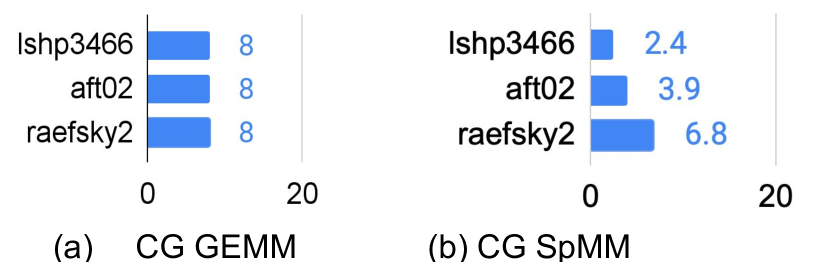
Figure 5: AI_best for (a) Conjugate Gradient skewed Dense GEMM and (b) Conjugate Gradient skewed SpMM operations for CG workloads. N=16, M,K and nnz vary by application.

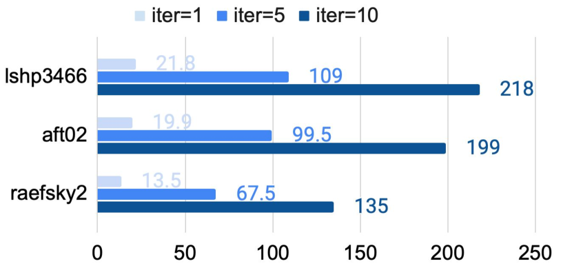
Figure 6: AI_best for full reuse across ’iter’ iterations of the CG loop.

Fig. 4 shows $AI_{best}$ for DNN workloads while  Fig. 5 shows the $AI_{best}$ of skewed SpMMs and Dense skewed GEMMs for CG workloads. The $A$ matrix for these workloads is obtained from suitesparse matrix collection [9]. Again, this data motivates the need to exploit inter-operation reuse to escape the memory bound.

Type	Einsum sequence	AIbest without inter-operation reuse	AIbest with inter-operation reuse
	$Z_{m,n}=\sum_{k}A_{m,k}*B_{k,n}$
	$Y_{o,n}=\sum_{j}C_{o,j}*Z_{j,n}$	$MNK+ONM+PON+QPN+RQN$	$MNK+ONM+PON+QPN+RQN$
NN	$X_{p,n}=\sum_{i}D_{p,i}*Y_{i,n}$	——————————————————————————————	———————————————-
like	$W_{q,n}=\sum_{h}E_{q,h}*X_{h,n}$	$MK+KN+2\times MN+OM+2\times ON+PO+2\times PN+QP+2\times QN+RQ+RN$	$MK+KN+OM+PO+QP+RQ+RN$
	$V_{r,n}=\sum_{g}F_{r,g}*W_{g,n}$
	$Z_{m,n}=\sum_{k}A_{m,k}*B_{k,n}$
	$Y_{o,n}=\sum_{j}C_{o,j}*Z_{j,n}$	$MNK+4\times ONM$	$MNK+4\times ONM$
HPC	$X_{m,n}=\sum_{i}Z_{m,i}*Y_{i,n}$	———————————————————————————–	———————————————-
like	$W_{o,n}=\sum_{h}Y_{o,h}*X_{h,n}$	$MK+KN+5\times MN+4\times OM+4\times ON$	$MK+KN+OM+MN$
	$V_{m,n}=\sum_{g}X_{m,g}*W_{g,n}$

Table 1: Arithmetic intensities of different sequences of Einsums with and without inter-operation reuse.

3.3 Inter-Operation Reuse

In a multi-Einsum scenario, we can increase intensity if we can avoid writing back the output of the first operation, and similarly avoid reading it in for the second. To show how much impact this can have, in  Table 1 we demonstrate the ideal inter-operation reuse potential for two chains of Einsums. The first is like a GNN and DNN where a new tensor is injected in every operation by the application (i.e., the layer’s weights). The second is like a solver where there are only three inputs and one output introduced by the application and intermediate tensors are reused locally between the Einsums.

Without inter-operation reuse and with execution at the operation granularity, the denominator which is the number of words, always consists of three tensors for every operation. Thus in the above example, with 5 Einsums, the denominator has 15 terms without inter-operation reuse. With inter-operation reuse, we only count each input once and the final output of the Einsum sequence. In NN-like case where a new weight is injected in every operation, there are six inputs $A,B,C,D,E,F$ and one final output $V$, thus 7 terms in the denominator. For an iterative HPC-like example, there are only 3 inputs from the application side $A,B,C$ and there is one final output $V$ leading to four terms in the denominator thus less traffic is injected by HPC application the application compared to NN. Thus, for a sequence of Einsums, the arithmetic intensity increases substantially if all the intermediate outputs are reused on-chip. For similar sized tensors, the arithmetic intensity improves by 2.14x and 3.75x respectively.

For low intensity individual operations with one large rank, if we assume that $N$ is the only large rank for all the sequence, $N\rightarrow\infty$, and consider all other ranks are equal, the arithmetic intensity without inter-operation reuse is $\frac{M}{2}$ for each case. With inter-operation reuse, the arithmetic intensity would be $\frac{5M}{2}$, increasing the intensity by 5x. Thus we observe through these examples, that an application with low intensity individual operation sequences can significantly benefit from inter-operation reuse.

As a practical example of CG, the $AI_{best}$ plots in  Fig. 6 uses loop unrolling to demonstrate that the complete Conjugate Gradient kernel can achieve a high AI_best, even though the, AI_best for each individual GEMM is limited. Unrolling of the loop (iter>1) and reusing the data amongst the unrolled iterations in Alg. 1 improves the intensity by huge amounts. However, loop unrolling is not a practical solution as it requires buffering extremely large amounts of data on-chip. Instead, we propose a mapping strategy that achieves substantial benefits even with realistic buffer sizes.

4 Exploiting Inter-Operation Reuse

This section discusses the inter-operation reuse opportunities in the the dependency graph of tensor operations using a systematic methodology. It formulates a generalized set of inter-operation reuse patterns in an arbitrary dependency graph of tensor operations. For the purpose of this paper, the graph is directed and acyclic.

4.1 Generalizing Inter-op reuse patterns

We identify five major inter-operation patterns in an arbitrary tensor DAG.

Sequential - The execution just takes place in an op-by-op function, although it maybe possible to reuse the data on-chip with Sequential pattern depending on the space in the buffer. There are generally no constraints on this type of pattern and this is the pattern used when none of the other patterns are possible. Also, this pattern does not give any benefit, and the output of the operation is both written and re-read from on-chip or off-chip depending on the capacity.

Pipelineable - A Pipelineable reuse pattern can exist at the edge connecting two consecutive nodes of the tensor dependency graph. This is shown as a blue arrow in Fig. 7. This implies that it would be possible and efficient to reduce the memory traffic using pipelining. This is the traditional pipelining used between the two operations in prior works [21, 12, 11, 35]. More than two operations could also be pipelined if the more than two consecutive nodes are connected by edges with pipelineable pattern. There are conditions to the pipelineable pattern. For an example pair of Einsums ${Z_{m,n}=\sum_{k}A_{m,k}*B_{k,n}}$ and ${W_{o,n}=\sum_{j}C_{o,j}*Z_{j,n}}$, if the contracted rank in the producer ie. $K$ and the unshared rank in the consumer ie. $O$ are dominant ranks, then pipelining is not beneficial and can lead to severe under-utilization since with $K$ being dominant, the consumer waits for a meaningful data and with $O$ being dominant, the producer waits for the consumer to consume the data. We discuss ’dominance’ further in Sec. 4.2. However, the pipelineable pattern does not guarantee pipelining unless additional conditions related to intra-operation dataflow are satisfied which we discuss in Sec. 5. If the intermediate tensor is no longer required, then pipelining gives the full benefit of having to avoid reading and writing the intermediate tensor into the memory. However, if the tensor $Z$ in the above example is required in the future, there is an additional need to perform pipeline_with_writeback or pipeline_with_hold.

Pipeline_with_writeback - Traditional operation pipelining completely consumes the intermediate tensor, and replaces it by the stage tensor, if the data is no longer needed. However, the intermediate tensor can be used in a future computation, a pattern that has not been observed in previously popular applications like Attention, Graph Neural Networks etc. This is represented by the transitive edge (discussed in Sec. 4.2) on the graph. Therefore this tensor needs to be stored in an on-chip SRAM buffer or DRAM depending on the capacity. This way, we need to write the tensor back to the SRAM/backing store but we still avoid having to read the tensor into the consecutive operation so it still provides half the benefit of  pipelineable pattern over the sequential pattern. Pipeline_with_writeback pattern can be seen in Conjugate Gradient as Fig. 7 shows in brick red color.

Pipeline_with_hold - As discussed above, we may need a pipelined tensor in the future. But there is a possibility that the complete chain until the future reuse of this tensor is pipelineable. In that case, we can bypass the requirement to write the complete tensor back into the backing store or the on-chip SRAM and we could just hold the tensor until the operation where we need to use the tensor reaches the particular stage. This essentially depends on the reuse distance between the operand nodes. This pattern provides the full benefit of pipelining but requires additional occupancy in the register file or on the on-chip SRAM depending on the granularity of pipelining. This pattern can be used in ResNet [15] residual block with skip connections as Fig. 7 shows in cyan color.

Parallel Multicast - It is also possible to reuse the a tensor into multiple parallel tensor operations, which we call Parallel_multicast. These parallel operations are non-transitive edges from the multicasting nodes to the directly connected nodes. This can be seen in Conjugate Gradient as Fig. 7 shows in green color.

4.2 Node and Edge Attributes of Dependency Graph

In this section, we discuss the various attributes of the nodes and the edges of the dependency graph that help determine the inter-operation reuse opportunities.

node.intra_dataflow: Dataflow within the operation that is represented by the node. It consists of loop order, parallelism and tiling strategies.

edge.inter_datflow: This represents one of the inter-operation patterns described in Sec. 4.1 except Parallel_multicast which is an attribute of the multicasting node and the non-transitive edges are marked automatically if the node is multicasting.

node.dominance: This is important in determining pipelining opportunities between the two operations since the source node is checked for contraction dominance and the destination node is checked for dominance of unshared rank. We define dominance in both relative terms and absolute terms since relative terms affect the pipelining stages and length of the stage while absolute terms affect the occupancy of the intermediate data. If a rank is greater than 1000 AND the ratio of the rank to the other ranks is more skewed than 100:1, the rank is considered as dominant. This attribute can take four values ’U’ (uncontracted rank is dominant), ’C’ (contracted rank is dominant), ’bal’ (All ranks are not too small and none of them is dominant, minimum value of the rank is 50) and ’small’ (all ranks are non-dominant and one of them is less than 50).

Critical Path/Longest path: It is the longest path between first and the last node. Intuitively, its the path that moves forward rather than branching out. $longestpath(edge)$ represents the portion of the critical path between source and destination node of that edge.

edge.isTransitive: This checks whether the edge is transitive or not. A transitive edge is an edge which is not on the critical path but the nodes it connects are on the critical path. For example, in the conjugate gradient iteration shown in Fig. 7, both the red edges are transitive edges, since they connect nodes on critical path but are not themselves on it. A transitive edge indicates an output of an operation that will be used later. For a pipelineable pattern, transitive edge represents the additional writeback or hold pattern.

node.numcast: The number of non-transitive edges originating from the node.

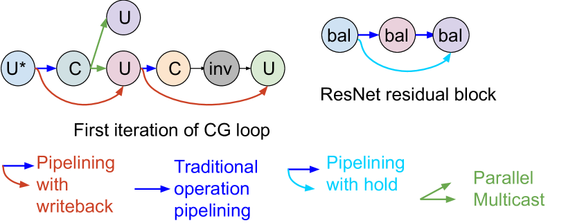
Figure 7: Output of Alg. 2 using colored edges. Letters in the node denote dominance, ’U’ means uncontracted, ’C’ means contracted and ’bal’ means all ranks are moderately big. Note that first tensor is uncontracted dominant since we compress the K rank (CSR format).

node.parallel_multicast: Represents that the node has parallel multicast opportunities for its output. All non-transitive edges from the node depict multicasting of the output to multiple operations and are colored green in Fig. 7.

edge.src and edge.dest: Represent the source and the destination nodes of the edge.

edge.tensor: The tensor represented by the edge.

node.op: The operation of the node. Tensor_mac denotes tensor multiplication or tensor addition/subtraction.

edge.tensor.ranks: Ranks of the edge.tensor

edge.tensor.swizzled: A tensor is swizzled when its read in the opposite order as it was previously written. For example, a tensor $P$ in row-major order but read in the N-major order is considered swizzled. A tensor is also said to be swizzled when the transpose is read in the same order as the tensor. For example, if the tensor $P$ with ranks M,N is written in an M-major order and $P^{T}$ is also read in the M-major order. Swizzling is determined from the relative order of the ranks in the loop order of the source and the destination of the edge. Swizzling of the shared ranks is unacceptable if the inter_dataflow of the edge is pipelineable or pipeline_with_hold. It incurs a penalty incase of pipeline_with_writeback which reduces the favorability of that dataflow due to reduction in locality. This is further discussed in Sec. 5.

4.3 Inter-operation Reuse Determination Algorithm

for node $\in$ NODES do

     node.numcast=0

     for edge $\in$ edges(node) do

         flag=0

         if edge.isTransitive == false then

             node.numcast++

             if node.numcast > 1 then

                 node.parallel_multicast=true

            

        if node.dominance$\neq$contracted$\And$edge.isTransitive==false then

             edge.inter_dataflow=pipelineable

        if node.dominance==contracted | node.op$\neq$tensor_mac then

             edge.inter_dataflow=sequential

        if edge.dest.dominance $\notin$ edge.tensor.ranks then

             edge.inter_dataflow=sequential

        if node.dominance$\neq$contracted$\And$edge.isTransitive==true then

             for pathnode $\in$ longestpath(edge) do

                 if pathnode.dominance==contracted then

                    edge.inter_dataflow=pipeline_with_writeback

                     flag=1

                     break

                

            if flag==0 then

                edge.inter_dataflow=pipeline_with_hold

            

        

    

Algorithm 2 Determination Inter-operation reuse opportunities for every edge in the DAG of tensor operations

Alg. 2 shows the methodology to mark the tensor dependency graph we reuse patterns. A node which has more than one non-transitive edges can multicast its output into more than one parallel operations and thus all the non-transitive edges from that node have the parllel_multicast pattern. A non-transitive edge where the source node is uncontracted dominant and the destination is unshared dominant, that edge has a pipelineable pattern. Note that pipelineable inter-operation pattern does not guarantee pipelining since it also depends on the order of the individual operations as we discuss in Sec. 5. Any edge where the source node is contracted dominant or the destination is unshared dominant, has a sequential inter-operation pattern. A transitive edge with uncontracted dominant source node could have Pipeline_with_hold pattern, if all the edges on the corresponding critical path are pipelienable, otherwise it has the Pipeline_with_writeback pattern.

Next, we focus on Gogeta mapping strategies for an arbitrary DAG of tensors.

5 Gogeta Mapping

In this section, we determine the dataflows and tile sizes of individual operations given that the dependency is marked with inter-operation reuse patterns. Through this we determine the entire mapping which we call Gogeta .

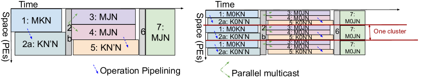
Figure 8: Example space-time representation of an iteration of Conjugate Gradient with loop orders. This is the set of loop orders with zero swizzle penalty. In the left chart, the overall compute is divided into multiple parts each executing one tensor. In the right chart, the tensors are split across the node by the dominant rank and the sub-tensors are pipelined within a cluster. Please refer to Alg. 1 for rank names. $M$ represents the large rank, $N$ ($\equiv N^{\prime}$) represents the small ranks. $K$ represents contractions of size $M$ and $J$ represents contractions of size $N$.

5.1 Loop order and Layouts

swizzle_penalty=0

for node $\in$ NODES do

     If the current node doesn’t have a dataflow, assign one

     If operation is not a tensor mul/add, skip to next node.

     for edge $\in$ edges(node) do

         if edge.dest.intra_dataflow==NOT ASSIGNED then

             if edge.inter_dataflow==pipelineable or

             edge.inter_dataflow==pipeline_with_hold then

                 dat=edge.src.intra_dataflow.loop_order

                 if dat[0] is contracted then

                     print("Loop order doesn’t adhere to pipelining")

                     Retry //Loop order is not pipelinable even if the edge is

                edge.dest.inter_dataflow.loop_order[0]=dat[0]

                 Pick the remaining ranks

                 Try a new order if swizzle penalty is high

            if node.parallel_multicast==true then

                 Assign same loop order to all non-transitive edges

                 First see if a node is already assigned

            if edge.inter_dataflow==pipeline_with_writeback or edge.inter_dataflow==sequential then

                 Pick an order that does not swizzle

            

        if edge.inter_dataflow==pipelineable or

        edge.inter_dataflow== pipeline_with_hold then

             if edge.src.intra_dataflow.loop_order[0] is contracted or edge.dest.intra_dataflow.loop_order[0] is unshared  then

                 print("Loop order doesn’t adhere to pipelining")

                 Retry //Loop order is not pipelinable even if the edge is

            if edge.tensor.swizzled then

                 print("Loop order doesn’t adhere to pipelining")

                 Retry //Loop order is not pipelinable even if the edge is

            

        

        if edge.inter_dataflow==pipeline_with_writeback or

        edge.inter_dataflow== sequential then

             if edge.tensor.swizzled then

                 swizzle_penalty++

            

        

    

if swizzle_penalty > $\epsilon$ then

    Retry

Algorithm 3 Determining the loop orders of the tensor operations to exploit reuse

In this section, we systematically determine the loop order of the individual tensors through Alg. 3 after the inter-operation reuse patterns have been marked as a result of Alg. 2. In Alg. 3, we determine the loop orders to make sure that we are able to pipeline where ever the inter-operation reuse pattern is pipelineable, which is important for low arithmetic intensity individual operations, and we retry with a new set of loop orders if a pipelineable edge cannot be pipelined due to the loop order pair of the source and the destination nodes.

For an example pair of Einsums $Z_{m,n}=\sum_{k}A_{m,k}*B_{k,n}$ and ${W_{o,n}=\sum_{j}C_{o,j}*Z_{j,n}}$. The conditions for pipelining a loop order pair are as follows-

• The edge connecting the nodes has a pipelineable inter-operation pattern.

• The source node has an uncontracted rank as the outermost loop. Having contraction ($K$) as the outermost loop implies that the complete sum that is usable by the next operation is generated at the very end.

• The destination node has a shared rank as the outermost loop. Having unshared rank ($O$) as the outermost loop implies that the shared tensor $Z$ is needed all over again when $o$ changes. But the idea of pipelining is to slice the intermediate tensor and consume it so that its not needed.

• The shared tensor $Z$ has the same order of ranks since the same portion of data that is produced, would be consumed. Thus no swizzling at that edge is allowed.

The algorithm ensures that each of the edges with pipelineable and pipeline_with_hold patterns have pipeline compatible loop orders. For parallel multicasting, the loop orders of all the nodes connecting the source node should be the same. The algorithm assigns the dataflow to the node with no assignment yet, based on pipelining and multicasting conditions. It also checks whether those conditions are met incase the dataflow was already assigned by some other incoming edge. It returns a retry if a pipelineable edge cannot be pipelined due to a certain loop order pair. In the Pipeline_with_writeback and Sequential case, it increases the penalty in case a tensor is swizzled, ie. read in an order different from which it was written in. If the swizzle penalty exceeds a threshold $\epsilon$, then the algorithm returns a retry. This threshold, could start from zero and gradually increase if we don’t find a set of loop orders.

This methodology guides the choice of loop orders which are pipeline compatible and have minimum possible swizzle penalty. For conjugate gradient, we determine a set of loop orders shown in Fig. 8. These orders have zero swizzle penalty with pipeline conditions satisfied and parallel_multicasted operations having same order wrt the multicasted tensor $\Lambda$ which is $MKN$ ie $P-$stationary and $S$-stationary respectively.

5.2 Tiling Strategy

Individual GEMMs: There are limited options for tiling individual low intensity skewed GEMMs because the non-dominant dimensions can become extremely low. Infact such GEMMs are often able to achieve the best possible data reuse with memory accesses $MK+KN+MN$ since the tensor made of the non-dominant ranks (for example, $\Lambda$ in line 3 and 4 of Alg. 1 and $\Gamma$ in line 5) can practically fit inside a portion of the Register File or parallelized across few PEs which means that the smaller tensor can just be streamed continuously from the RF while the large tensor is stationary. However, as discussed in Sec. 3, even the best intensity is extremely low for the skewed GEMMs .

Considering multiple GEMMs: With pipelining and parallel_multicast, there are different ways in which data can be communicated spatially. Assuming multiple clusters of sub-accelerators, one could pipeline by having the whole tensor be local and occupy the two halves of compute entirely. Prior works like [33, 11] have divided the substrate into large chunks for each tensor just like Fig. 8 left shows. The major disadvantage of that would be a significant sized tensor being communicated through the inter-cluster NoC which usually has lower bandwidth than the intra-cluster NoC. On the other hand, for skewed GEMMs, which do not have significant intra-operation reuse anyway, we propose to slice the dominant rank on multiple clusters instead and have the tensors be pipelined within a cluster as Fig. 8 right shows. When the dominant rank is split ($M$ for example in line 4 of Alg. 1) the chunks would share the small tensor formed by non-dominating ranks($\Lambda$) and $\Gamma$. Broadcasting $\Lambda$ and reducing $\Gamma$ on the inter-cluster NoC has orders of magnitude less communication on the inter-cluster NoC compared to communicating $R$ between clusters.

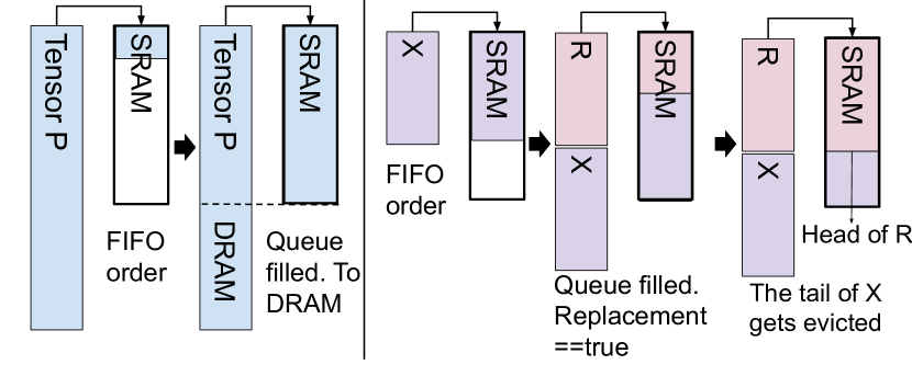
Figure 9: Data organization in the SRAM. Left shows SRAM filling up without replacement. The part that could not fit is sent to DRAM. Right part shows that after queue is filled, the tail of $X$ is evicted and next element of $R$ is enqueued at the head to fill the space.

5.3 Data organization in SRAM

There are various scenarios regarding the amount of tensors the SRAM can hold ranging from a fraction to multiple tensors depending on the workload size and the architecture. In Gogeta , we choose the loop orders to minimize the swizzling of ranks in a tensor. Due to this, we write the tensor in FIFO order and if the SRAM is full, we send the remaining portion of that tensor to DRAM as Fig. 9 shows. This makes sure that we access the portion of the tensor in the SRAM first rather than replacing it by the later part of the tensor and again reading the earlier part. If the tensor fits, we can repeat this for multiple operations. We read the tensor at the head.

While this makes sure that we minimize the off-chip traffic for that particular tensor, there is still a chance that a particular tensor which is not reused until later (for example, $X$ in line 3 of Alg. 1 which is used in line 3 of the next iteration) is written to SRAM at the expense of a future tensor that is used before the reuse of the previous tensor (for example $R$ in line 4 which is reused in lines 5 and 7 of the same iteration). In that case, based on the reuse distance, we prioritize $R$ and evict out a portion of $X$ to make room for $R$ by evicting the later elements of $X$ first. Then $R$ is read at its head. This is the first work to the best of our knowledge that considers reuse distance and frequency of a tensor in the dependency graph and proposed data organization strategies at a tensor granularity.

If 3 and 4 were executed in parallel as Fig. 8 shows, $R$ and $X$ would occupy equal halves in the second step and the later part of $R$ will eventually replace the tail of earlier part of $X$ and the later part of $X$ would be sent straight to DRAM, resulting in the same proportions of $R$ and $X$.

6 Evaluations

6.1 Experimental Methodology

We describe our experimental methodology for demonstrating the efficiency of Gogeta across baseline dataflows. We focus on the inter-cluster communication and the DRAM accesses which is same regardless of microarchitectural parameters.

6.1.1 Analytical Framework

We build an analytical model to capture the memory accesses and communication across clusters for the baselines and Gogeta to compare the achieved arithmetic intensity of the dataflows independent of the accelerator implementation. We validate the data movement statistics for a single layer by using STONNE [26], which is a cycle accurate simulator that models one DNN layer at a time and models flexible interconnects [24] with ability to support multiple intra-operation dataflows. STONNE has been validated against MAERI [24] and SIGMA [30] RTLs. We validated the data movement for a pair of two pipelined tensor operations using OMEGA [12, 2] which is a wrapper around STONNE to model pipelining between two operations.

6.1.2 Workloads and Datasets

Table 2: Workloads and Datasets evaluated. Protein is a graph classification dataset and we classify a batch of 64 graphs similar to OMEGA. ’nnz’ stands for number of non zeros in $M\times M$ matrix. The ranks M,N,O are the ones described in the Einsums in Sec. 2.2. For Conjugate Gradients, we sweep N as a parameter as discussed in Sec. 6.1.4.

Workload	Dataset	Shapes and Sparsity
	aft02	M=8184, nnz=127762
Conjugate	ecology1	M=1000000, nnz=4996000
Gradient	Barth5	M=15606, nnz=61484
	Nasa4704	M=4704, nnz=104756
GCN	cora	M=2708, nnz=9464, N=1433, O=7
Layer	protein*	M=3786, nnz=14456, N=29, O=2

We evaluate our methodology and the Gogeta mapping strategy for Conjugate Gradient and GNN (GNN results in Sec. 6.2.2). We obtain the sparse matrices of the Conjugate Gradient Datasets from Suitesparse [9] for scientific problems like structural problems, stencils, acoustics etc. We obtain GNN graphs from OMEGA [2].

6.1.3 Dataflow Configurations

Table 3: Dataflow Configurations

Config	Description
SEQ-Flex	Op-by-op with best possible mapping per layer.
	Operands begin and end in DRAM.
SEQ-Overflow	SEQ-Flex but only the portion of the operands
	overflowing get written to the DRAM.
GOGETA-df	GOGETA dataflow with inter-op pattern Alg. 2
GOGETA-map	GOGETA-df with tiling strategy in Sec. 5.2
Ideal	Infinite SRAM and prefect inter-operation reuse

We compare multiple dataflow configurations described in Table 3. SEQ-Flex dataflow has the lowest possible DRAM accesses for individual layers but it considers the output tensor of each operation ending up in the DRAM and the input coming from the DRAM. SEQ-Overflow dataflow considers that the data is written in the SRAM and the portion that does not fit is sent to the DRAM. To make the baseline strong and fair, we writeback the tensor in FIFO order (but do not consider reuse distance based replacement) in SEQ-Overflow. GOGETA-df uses inter-op patterns to reduce pressure on memory and finds the individual loop order with pipelining and also avoids swizzle_penalty. GOGETA-map also uses the scalable tiling strategy that reduces inter-cluster communication overhead in addition to GOGETA-df. GOGETA-df and GOGETA-map also include the tensor allocation strategy of FIFO order write and reuse distance based replacement in Sec. 5.3. Ideal, represents the DRAM accesses with perfect reuse.

6.1.4 Workload and Architecture Parameters

Table 4: Configurations for workloads and architecture

Parameter	Value
Bytes per word/element	4B (32 bits)
Iterations of CG loop	10
N rank in CG	Sweep: 1, 8, 16
Number of PEs per cluster	1024
Number of clusters	16
Total SRAM capacity	Sweep: 1MB, 4MB, 16MB
Register file capacity	0.5KB per PE

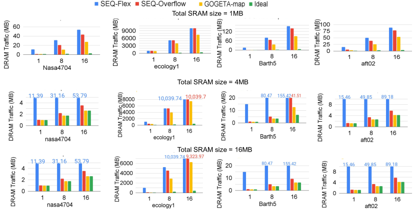
Figure 10: DRAM data movement in Megabytes for N (x-axis) = 1, 8, 16 and SRAM sizes, 1MB, 4MB and 16MB. We cut the Y-axis at a lesser value for certain plots due to large disparity between SEQ-Flex and GOGETA-map.

Table 4 describes the architecture configuration we use for the evaluation and the parameters we sweep. We run workloads of different sizes and nnz’s and we also sweep the $N$ rank that corresponds to number of simultaneous initial guesses and the SRAM size to capture different scenarios with varying ratios of tensor and SRAM sizes. We consider a clustered architecture, each cluster of 1024 PEs backed by its own SRAM slice.

6.2 Results

6.2.1 DRAM accesses in Conjugate Gradient

We evaluate the DRAM accesses for Conjugate Gradient for the workloads and datasets in Sec. 6.1.2 as  Fig. 10 shows. We achieve a geomean of 6.7x reduction in DRAM traffic over the Seq-Flex baseline, ranging from 1.18x to 23.7x.

For a dataset with tensors smaller than the SRAM size for example, aft02 and nasa4704 at 4/16 MB SRAM, Gogeta hits the ideal (perfect reuse) DRAM accesses. For such cases SEQ-Overflow which uses a FIFO order write policy as demonstrated in Sec. 5.3, also achieves a close performance but Gogeta performs better due to the ability to use the same tensor for transpose as well.

For extremely large datasets like ecology1, for small memory size, SEQ-Flex and SEQ-Overflow incur similar DRAM accesses and Gogeta performs 18 to 30% better than Sequential baselines due to pipelining_with_writeback which avoids reading the operand from the DRAM for the consecutive operation. In such large workloads, pipelining plays a major role in reducing the off-chip traffic.

For all the intermediate datapoints, where some but not all tensors fit the SRAM, there is a clear downward trend between SEQ-Flex, SEQ-Overflow and Gogeta in terms of DRAM accesses. This is due to a combination of multiple reasons, including pipelining_with_writeback, ability to organize data in the SRAM based on reuse distance of downstream tensor operations and the ability to achieve zero swizzle penalty.

Thus Gogeta achieves better performance than the Sequential baselines due to pipelining, swizzle aware loop ordering and due to data organization strategy. We also evaluate DRAM accesses for Graph Neural Networks in Sec. 6.2.2 to demonstrate the generality of Gogeta .

6.2.2 DRAM accesses in GNNs

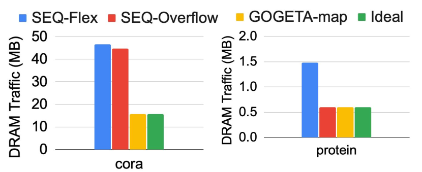
Figure 11: Data movement for Graph Neural Networks.

To demonstrate the generality across applications, we also show the DRAM accesses for a GCN layer for graphs with chemistry applications. GCN layer consists of two operations with a pipelienable reuse pattern between them. We evaluate them for SRAM size of 1MB as Fig. 11 shows.

Cora has a large feature matrix $M\times N$ but still has low arithmetic intensity due to low number of non zeros per row. There is a marginal improvement in SEQ with overflow but considerable improvement with pipelining and hits the ideal. Protein dataset is relatively small and the tensors fit in the SRAM, thus both SEQ-Overflow and GOGETA-map hit the ideal. Graph Neural Network layers do not have downstream tensors using the same data thus pipelining makes it easier to achieve the ideal DRAM accesses.

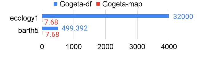
Figure 12: Inter-cluster NoC link traversals in KBs for N=8. We cap the x-axis due to high range.

6.2.3 Communication analysis of Tiling

:

If we consider operations 4 and 5 in CG (Alg. 1), the total traversals on the inter-cluster NoC for GOGETA-df is $sizeof(R)$ which is $M\times N$ even if these operations are allocated such that they are 1 hop apart which leads to considerable delay and energy since inter-cluster bandwidth ($\equiv$ inter-chiplet) is low compared to in-cluster bandwidth. Instead, if we use GOGETA-map where pipelining happens inside the cluster and $M$ rank is sliced across the clusters, maximum inter-cluster link traversals are $sizeof(\Lambda)\times Broadcast~{}traversals$ + $sizeof(\Gamma)\times Reduce~{}traversals$ which is $2\times N\times N\times 15$ ($N\times N$ data moved through at most 15 links for broadcast and reduction) for 16 clusters. Fig. 12 shows inter-cluster link traversal for GOGETA-df and GOGETA-map in KB’s. Workload can scale up considerably and the dimension that will scale is $M$. By changing these to intra-cluster traversals, GOGETA-map makes better use of high bandwidth NoC.

7 Discussion and Future Work

HPC/scientific applications are interesting because of the extreme demands they put on our hardware systems. Ideally, those applications would be made up of kernels that can be independently analyzed and optimized, then composed together into dependency graphs. In this paper we demonstrate that this individual operation view is too limited in scope: there is major opportunity to improve optimization by using an inter-operation viewpoint to increase arithmetic intensity.

We have demonstrated that Gogeta can apply in scenarios where traditional loop fusion and unrolling are not sufficient. We demonstrate a geomean 6.7x reduction in memory accesses across a range of data sets and buffer sizes. Today, existing mapping tools such as Timeloop [28] focus on single Einsum optimization. We hope that integrating the Gogeta algorithm directly into their toolflow will allow a broad audience to exploit inter-operation reuse.

References

- [1] HPCG Benchmark 2021. https://www.hpcg-benchmark.org/custom/index.html?lid=155&slid=311.
- [2] OMEGA. https://github.com/stonne-simulator/omega.
- [3] NVDLA deep learning accelerator. http://nvdla.org, 2017.
- [4] Taco: The tensor algebra compiler. http://tensor-compiler.org/, 2021.
- [5] Bahar Asgari, Ramyad Hadidi, Tushar Krishna, Hyesoon Kim, and Sudhakar Yalamanchili. Alrescha: A lightweight reconfigurable sparse-computation accelerator. In 2020 IEEE International Symposium on High Performance Computer Architecture (HPCA), pages 249–260. IEEE, 2020.
- [6] Yu-Hsin Chen, Joel Emer, and Vivienne Sze. Eyeriss: A spatial architecture for energy-efficient dataflow for convolutional neural networks. In Proceedings of the 43rd International Symposium on Computer Architecture, ISCA ’16, page 367–379. IEEE Press, 2016.
- [7] Yu-Hsin Chen, Tien-Ju Yang, Joel Emer, and Vivienne Sze. Eyeriss v2: A flexible accelerator for emerging deep neural networks on mobile devices. IEEE Journal on Emerging and Selected Topics in Circuits and Systems, 9(2):292–308, 2019.
- [8] Siegfried Cools and Wim Vanroose. The communication-hiding pipelined bicgstab method for the parallel solution of large unsymmetric linear systems. Parallel Computing, 65:1–20, 2017.
- [9] Timothy A. Davis and Yifan Hu. The university of florida sparse matrix collection. ACM Trans. Math. Softw., 38(1), dec 2011.
- [10] Jack Dongarra, Michael A Heroux, and Piotr Luszczek. Hpcg benchmark: a new metric for ranking high performance computing systems. Knoxville, Tennessee, page 42, 2015.
- [11] Mingyu Gao, Xuan Yang, Jing Pu, Mark Horowitz, and Christos Kozyrakis. Tangram: Optimized coarse-grained dataflow for scalable nn accelerators. In Proceedings of the Twenty-Fourth International Conference on Architectural Support for Programming Languages and Operating Systems, ASPLOS ’19, page 807–820, New York, NY, USA, 2019. Association for Computing Machinery.
- [12] Raveesh Garg, Eric Qin, Francisco Muñoz-Martínez, Robert Guirado, Akshay Jain, Sergi Abadal, José L Abellán, Manuel E Acacio, Eduard Alarcón, Sivasankaran Rajamanickam, and Tushar Krishna. Understanding the design-space of sparse/dense multiphase gnn dataflows on spatial accelerators. In 2022 IEEE International Parallel and Distributed Processing Symposium (IPDPS), 2022.
- [13] Will Hamilton, Zhitao Ying, and Jure Leskovec. Inductive representation learning on large graphs. In Advances in neural information processing systems, pages 1024–1034, 2017.
- [14] Song Han, Xingyu Liu, Huizi Mao, Jing Pu, Ardavan Pedram, Mark A. Horowitz, and William J. Dally. Eie: Efficient inference engine on compressed deep neural network. In Proceedings of the 43rd International Symposium on Computer Architecture, ISCA ’16, page 243–254. IEEE Press, 2016.
- [15] K. He et al. Deep Residual Learning for Image Recognition. In CVPR, 2016.
- [16] Kartik Hegde, Hadi Asghari-Moghaddam, Michael Pellauer, Neal Crago, Aamer Jaleel, Edgar Solomonik, Joel Emer, and Christopher W. Fletcher. Extensor: An accelerator for sparse tensor algebra. In Proceedings of the 52nd Annual IEEE/ACM International Symposium on Microarchitecture, MICRO ’52, page 319–333, New York, NY, USA, 2019. Association for Computing Machinery.
- [17] Magnus Rudolph Hestenes, Eduard Stiefel, et al. Methods of conjugate gradients for solving linear systems. NBS Washington, DC, 1952.
- [18] Qijing Huang, Minwoo Kang, Grace Dinh, Thomas Norell, Aravind Kalaiah, James Demmel, John Wawrzynek, and Yakun Sophia Shao. Cosa: Scheduling by <u>c</u>onstrained <u>o</u>ptimization for <u>s</u>patial <u>a</u>ccelerators. In Proceedings of the 48th Annual International Symposium on Computer Architecture, ISCA ’21, page 554–566. IEEE Press, 2021.
- [19] Norman P. Jouppi, , Cliff Young, Nishant Patil, David Patterson, Gaurav Agrawal, Raminder Bajwa, Sarah Bates, Suresh Bhatia, Nan Boden, Al Borchers, Rick Boyle, Pierre luc Cantin, Clifford Chao, Chris Clark, Jeremy Coriell, Mike Daley, Matt Dau, Jeffrey Dean, Ben Gelb, Tara Vazir Ghaemmaghami, Rajendra Gottipati, William Gulland, Robert Hagmann, C. Richard Ho, Doug Hogberg, John Hu, Robert Hundt, Dan Hurt, Julian Ibarz, Aaron Jaffey, Alek Jaworski, Alexander Kaplan, Harshit Khaitan, Daniel Killebrew, Andy Koch, Naveen Kumar, Steve Lacy, James Laudon, James Law, Diemthu Le, Chris Leary, Zhuyuan Liu, Kyle Lucke, Alan Lundin, Gordon MacKean, Adriana Maggiore, Maire Mahony, Kieran Miller, Rahul Nagarajan, Ravi Narayanaswami, Ray Ni, Kathy Nix, Thomas Norrie, Mark Omernick, Narayana Penukonda, Andy Phelps, Jonathan Ross, Matt Ross, Amir Salek, Emad Samadiani, Chris Severn, Gregory Sizikov, Matthew Snelham, Jed Souter, Dan Steinberg, Andy Swing, Mercedes Tan, Gregory Thorson, Bo Tian, Horia Toma, Erick Tuttle, Vijay Vasudevan, Richard Walter, Walter Wang, Eric Wilcox, and Doe Hyun Yoon. In-datacenter performance analysis of a tensor processing unit. In Proceedings of the 44th Annual International Symposium on Computer Architecture (ISCA), 2017.
- [20] Sheng-Chun Kao and Tushar Krishna. Gamma: automating the hw mapping of dnn models on accelerators via genetic algorithm. In 2020 IEEE/ACM International Conference On Computer Aided Design (ICCAD), pages 1–9. IEEE, 2020.
- [21] Sheng-Chun Kao, Suvinay Subramanian, Gaurav Agrawal, and Tushar Krishna. An optimized dataflow for mitigating attention performance bottlenecks. arXiv preprint arXiv:2107.06419, 2021.
- [22] Thomas N. Kipf and Max Welling. Semi-supervised classification with graph convolutional networks. ICLR, 2017.
- [23] Hyoukjun Kwon, Prasanth Chatarasi, Michael Pellauer, Angshuman Parashar, Vivek Sarkar, and Tushar Krishna. Understanding reuse, performance, and hardware cost of dnn dataflow: A data-centric approach. In Proceedings of the 52nd Annual IEEE/ACM International Symposium on Microarchitecture, pages 754–768. ACM, 2019.
- [24] Hyoukjun Kwon, Ananda Samajdar, and Tushar Krishna. MAERI: enabling flexible dataflow mapping over dnn accelerators via programmable interconnects. In Proceedings of the Twenty-Third International Conference on Architectural Support for Programming Languages and Operating Systems, page 461–475. ACM, 2018.
- [25] Shengwen Liang, Ying Wang, Cheng Liu, Lei He, LI Huawei, Dawen Xu, and Xiaowei Li. Engn: A high-throughput and energy-efficient accelerator for large graph neural networks. IEEE Transactions on Computers, 2020.
- [26] Francisco Muñoz-Matrínez, José L. Abellán, Manuel E. Acacio, and Tushar Krishna. Stonne: Enabling cycle-level microarchitectural simulation for dnn inference accelerators. In 2021 IEEE International Symposium on Workload Characterization (IISWC), 2021.
- [27] Wei Niu, Jiexiong Guan, Yanzhi Wang, Gagan Agrawal, and Bin Ren. DNNFusion: Accelerating Deep Neural Networks Execution with Advanced Operator Fusion. In PLDI, 2021.
- [28] Angshuman Parashar, Priyanka Raina, Yakun Sophia Shao, Yu-Hsin Chen, Victor A. Ying, Anurag Mukkara, Rangharajan Venkatesan, Brucek Khailany, Stephen W. Keckler, and Joel Emer. Timeloop: A systematic approach to dnn accelerator evaluation. In 2019 IEEE International Symposium on Performance Analysis of Systems and Software (ISPASS), pages 304–315, 2019.
- [29] Raghu Prabhakar, Yaqi Zhang, David Koeplinger, Matt Feldman, Tian Zhao, Stefan Hadjis, Ardavan Pedram, Christos Kozyrakis, and Kunle Olukotun. Plasticine: A reconfigurable architecture for parallel paterns. In Proceedings of the 44th Annual International Symposium on Computer Architecture, ISCA ’17, page 389–402, New York, NY, USA, 2017. Association for Computing Machinery.
- [30] Eric Qin, Ananda Samajdar, Hyoukjun Kwon, Vineet Nadella, Sudarshan Srinivasan, Dipankar Das, Bharat Kaul, and Tushar Krishna. Sigma: A sparse and irregular gemm accelerator with flexible interconnects for dnn training. In 2020 IEEE International Symposium on High Performance Computer Architecture (HPCA), pages 58–70, 2020.
- [31] Kamil Rocki, Dirk Van Essendelft, Ilya Sharapov, Robert Schreiber, Michael Morrison, Vladimir Kibardin, Andrey Portnoy, Jean Francois Dietiker, Madhava Syamlal, and Michael James. Fast stencil-code computation on a wafer-scale processor. In SC20: International Conference for High Performance Computing, Networking, Storage and Analysis, pages 1–14. IEEE, 2020.
- [32] Youcef Saad and Martin H. Schultz. Gmres: A generalized minimal residual algorithm for solving nonsymmetric linear systems. SIAM Journal on Scientific and Statistical Computing, 7(3):856–869, 1986.
- [33] Yakun Sophia Shao, Jason Clemons, Rangharajan Venkatesan, Brian Zimmer, Matthew Fojtik, Nan Jiang, Ben Keller, Alicia Klinefelter, Nathaniel Pinckney, Priyanka Raina, Stephen G. Tell, Yanqing Zhang, William J. Dally, Joel Emer, C. Thomas Gray, Brucek Khailany, and Stephen W. Keckler. Simba: Scaling deep-learning inference with multi-chip-module-based architecture. In Proceedings of the 52nd Annual IEEE/ACM International Symposium on Microarchitecture, MICRO ’52, page 14–27, New York, NY, USA, 2019. Association for Computing Machinery.
- [34] Henk A Van der Vorst. Bi-cgstab: A fast and smoothly converging variant of bi-cg for the solution of nonsymmetric linear systems. SIAM Journal on scientific and Statistical Computing, 13(2):631–644, 1992.
- [35] Mingyu Yan, Lei Deng, Xing Hu, Ling Liang, Yujing Feng, Xiaochun Ye, Zhimin Zhang, Dongrui Fan, and Yuan Xie. Hygcn: A gcn accelerator with hybrid architecture. In 2020 IEEE International Symposium on High Performance Computer Architecture (HPCA), pages 15–29, 2020.
- [36] Xuan Yang, Mingyu Gao, Qiaoyi Liu, Jeff Setter, Jing Pu, Ankita Nayak, Steven Bell, Kaidi Cao, Heonjae Ha, Priyanka Raina, Christos Kozyrakis, and Mark Horowitz. Interstellar: Using halide’s scheduling language to analyze dnn accelerators. In Proceedings of the Twenty-Fifth International Conference on Architectural Support for Programming Languages and Operating Systems, ASPLOS ’20, page 369–383, New York, NY, USA, 2020. Association for Computing Machinery.
- [37] T. Young, D. Hazarika, S. Poria, and E. Cambria. Recent trends in deep learning based natural language processing [review article]. IEEE Computational Intelligence Magazine, 13(3):55–75, 2018.