Data-Driven Exact Pole Placement for Linear Systems

Abstract

The exact pole placement problem concerns computing a feedback gain that will assign the poles of a system, controlled via static state feedback, at a set of pre-specified locations. This is a classic problem in feedback control and numerous methodologies have been proposed in the literature for cases where a model of the system to control is available. In this paper, we study the problem of computing feedback gains for pole placement (and, more generally, eigenstructure assignment) directly from experimental data. Interestingly, we show that the closed-loop poles can be placed exactly at arbitrary locations without relying on any model description but by using only finite-length trajectories generated by the open-loop system. In turn, these findings imply that classical control objectives, such as feedback stabilization or meeting transient performance specifications, can be achieved without first identifying a system model. Numerical experiments demonstrate the benefits of the data-driven pole-placement approach as compared to its model-based counterpart.

I Introduction

Data-driven control methods enable the synthesis of feedback controllers directly from historical data generated by a physical systems, and thus elude the need to construct or identify a model for the underlying system to control. Data-driven approaches are especially useful in scenarios where first-principle models are difficult to derive or the identification task may lead to numerically-unreliable model parametrizations [1, 2]. In these cases, data-driven methods set out a huge potential since controllers can be synthesized directly from data, and thus possible uncertainties in the identified model parameters shall not propagate when these parameters are used for control design.

Data-driven control synthesis is, by now, a well-investigated area of research (see, e.g., the representative works [3, 4, 5]). Despite the availability of several techniques to synthesize various types of controllers from data, to the best of our knowledge, the problem of data-driven pole placement and the (more general) problem of data-driven eigenstructure assignment via static feedback have not been studied until now. The classical problem of pole placement consists in finding a static feedback gain matrix such that the poles of the closed-loop system are in a set of pre-specified locations; analogously, the problem of eigenstructure assignment is that of finding a static feedback gain such that the closed-loop system has a pre-specified set of eigenvalues and eigenvectors (hereafter named eigenstructure). Motivated by this background, in this paper we study the data-driven pole placement problem and the data-driven eigenstructure assignment problem. Our results show that it is possible to place the closed-loop eigenvalues exactly at arbitrary locations (in this context, “exactly” means that the closed-loop poles can be placed at exact locations, in contrast with cases where they can placed within certain regions) by using formulas that can be applied directly on data. Moreover, our results show that the data-driven eigenstructure assignment problem is feasible under the same conditions required for its model-based counterpart.

Paper contributions. This paper features two main contributions. First, we show that static feedback gains that place the poles at an arbitrary set of locations can be computed directly from data collected from finite-length open-loop control experiments. We remark that our formulas apply also to cases where the open-loop system is not stable. We provide an explicit formula to compute the feedback gain and we show that the problem is always feasible when the underlying system is controllable. Second, we study the eigenstructure assignment problem and we provide a necessary and sufficient condition to check when such a problem is feasible. Moreover, we provide an explicit formula to compute feedback gains that assign a pre-specified eigenstructure. Finally, as a minor contribution, we evaluate via numerical simulations the benefits of the proposed data-driven method as compared to model-based approaches.

Related work. Several techniques have been proposed to synthesize controllers from data while avoiding the need to identify the system model. Solutions for static feedback control are studied in [6, 7], the linear quadratic regulator (LQR) in [3], model predictive control (MPC) in [5, 8], minimum-energy control laws in [4], trajectory tracking problems in [9], distributed control problems in [11], and feedback-optimization controllers are proposed in [10]. Some extensions to the case of nonlinear systems are presented in [12, 13]. Most of these methods exploit the ability to express future trajectories of a linear system in terms of a sufficiently-rich past trajectory, as shown by the Fundamental Lemma [14]. With respect to this body of literature, in this work, we focus on the exact pole-placement problem.

The model-based exact pole placement problem has a long history; a non-exhaustive list of references includes [15, 16, 17, 18]. However, all these classical methods construct on a model-based description of the system to control; in contrast with these methods, our focus here is to derive formulas for pole placement that can be applied directly on data. In line with this work is the recent contribution [19], where the authors study the problem of placing the closed-loop poles in linear matrix inequality (LMI) regions; in contrast, in this work, we focus on placing the poles at exact locations and, moreover, we address the eigenstructure assignment problem.

II Preliminaries

In this section, we recall some useful facts on behavioral system theory from [14]. Given a signal (time-series) $z:\mathbb{Z}\rightarrow{}^{\sigma}$, and scalars $T\in\mathbb{Z}_{\geq 0}\cup\{+\infty\}$, $i\in\mathbb{Z}_{\geq 0},i\leq T$, we denote the restriction of $z$ to the interval $[i,i+T-1]$ by $z_{[i,i+T-1]}:=\{z(i),\dots,z({i+T-1})\}$ (notice that $z_{[i,i+T-1]}$ is a $T$-long signal). With a slight abuse of notation, we will also denote by $z_{[i,i+T-1]}:=(z(i),\dots,z({i+T}))\in{}^{\sigma T}$ the vectorization of the signal $z_{[i,i+T-1]}$, where the distinction will be clear from the context. Given the $T-$long signal $z_{[i,i+T-1]}$, we denote the associated Hankel matrix with $L$ (block) rows by: $\displaystyle\mathcal{H}_{L}(z_{[i,i+T-1]})=\begin{bmatrix}z(i)&z(i+1)&\ldots&z(i+T-L)\\ z(i+1)&z(i+2)&\ldots&z(i+T-L+1)\\ \vdots&\vdots&\ddots&\vdots\\ z(i+L\scalebox{0.75}[0.9]{$-$}1)&z(i+L)&\ldots&z(i+T-1)\end{bmatrix},$ Notice that $\mathcal{H}_{L}(z_{[i,i+T]})\in{}^{L\sigma\times(T-L+1)}$. The following definition is instrumental for our analysis.

Definition II.1

(Persistently Exciting Signal [14]) The signal $z_{[i,i+T-1]}\in{}^{\sigma}$ is persistently exciting of order $L$ if the matrix $\mathcal{H}_{L}(z_{[i,i+T-1]})$ has full row rank $\sigma L$. $\square$

We note that persistence of excitation implicitly requires that the number of columns of $\mathcal{H}_{L}(z_{[i,i+T-1]})$ is non-smaller than the number of rows, or $T-L+1\geq L\sigma$.

We recall the following properties of linear dynamical systems subject to a persistently exciting input.

Lemma II.2

(Fundamental Lemma [14, Thm 1]) Assume that the linear system $x(t+1)=Ax(t)+Bu(t)$ is controllable and let $(u_{[0,T-1]},x_{[0,T-1]})$ be an input-state trajectory generated by this system. If $u_{[0,T-1]}$ is persistently exciting of order $n+d$, then:

$$\operatorname{rank}\begin{bmatrix}\mathcal{H}_{1}(x_{[0,T-1]})\\ \mathcal{H}_{d}(u_{[0,T-1]})\end{bmatrix}=n+dm.$$

$\Box$

This condition will play a fundamental role in the sequel.

III Problem setting

In this section, we formulate the problem of interest and discuss existing (model-based) techniques for its solution.

III-A Problem formulation

Consider the discrete-time linear time-invariant system:

$$x(t+1)=Ax(t)+Bu(t),$$ (1)

where $A\in{}^{n\times n}$ and $B\in{}^{n\times m}$ denote, respectively, the system and input matrices, and $x:\mathbb{Z}_{\geq 0}\rightarrow{}^{n}$ and $u:\mathbb{Z}_{\geq 0}\rightarrow{}^{m}$ denote, respectively, the state and input signals. We assume that $B$ has full column rank. The behavior of (1) is governed by the poles of the system, that is, by the eigenvalues of $A$. It is often desirable to modify the poles of the system to obtain certain properties, such as system stability or a desired transient performance. This can be achieved by using a state-feedback control law of the form $u(t)=-Kx(t)+v(t),$ where $v:\mathbb{Z}_{\geq 0}\rightarrow{}^{m}$ is a new free input and $K\in{}^{m\times n}$ is called feedback gain, which should be chosen so that the controlled system

$$x(t+1)=(A-BK)x(t)+v(t),$$ (2)

has the desired poles. In line with [15, 16, 17, 18], we make the following assumption.

Assumption 1 (Desired set of pole locations)

The set of desired pole locations contains $n$ complex numbers $\mathcal{L}=\{\lambda_{1},\dots,\lambda_{n}\}$ and is closed under complex conjugation. $\square$

The data-driven state-feedback pole placement problem is then formulated precisely as follows.

Problem 1 (Pole placement)

Given a set of complex numbers $\mathcal{L}$ satisfying Assumption 1 and historical data $\mathcal{D}=(u_{[0,T-1]},x_{[0,T-1]})$ generated by (1), find, when possible, a matrix $K\in{}^{m\times n}$ such that the eigenvalues of $A-BK$ are the elements of the set $\mathcal{L}$. $\square$

Conditions for the existence of solutions to the pole placement problem are well known [20]: a solution exists if and only if $\mathcal{L}$ contains all uncontrollable modes [20] of $(A,B).$ Thus, we will make the following assumption.

Assumption 2 (Controllability)

All modes of $(A,B)$ are controllable. $\square$

In the single-input case ($m=1$), the solution to Problem 1, when it exists, is unique [20]. In the multi-input case $1<m<n$, the feedback gain $K$ that solves the pole placement problem is in general non-unique. One common way to select a particular $K$ within the ambiguity set is to choose the one that assigns the closed-loop eigenstructure:

$$(A-BK)X=X\Lambda,$$ (3)

where $\Lambda$ is an $n\times n$ diagonal matrix with spectrum given by $\mathcal{L}$ and $X$ is a non-singular matrix of associated closed-loop eigenvectors, chosen according to some notion of optimality. For instance, the authors in[16, Sec. 2.5] show that choosing a matrix of eigenvectors $X$ that is well-conditioned leads to pole locations that are robust against perturbations of the entries of $A$. Motivated by this, in this paper we consider the data-driven state-feedback eigenstructure assignment problem, formulated precisely as follows.

Problem 2 (Eigenstructure assignment)

Given a set of complex numbers $\mathcal{L}$ satisfying Assumption 1, a matrix of linearly independent eigenvectors $X,$ and historical data $\mathcal{D}=(u_{[0,T-1]},x_{[0,T-1]})$ generated by (1), find, when possible, a matrix $K\in{}^{m\times n}$ such that (3) holds. $\square$

III-B Existing model-based pole-placement methods

Several formulas have been proposed in the literature to solve the pole placement and eigenstructure assignment problems. Next, we will summarize some of the most celebrated. In what follows, we denote by $M^{\dagger}$ the Moore-Penrose inverse of matrix $M.$

1. Approach in [16, Thm 3]. Let $B=\begin{bmatrix}U_{0},&U_{1}\end{bmatrix}\begin{bmatrix}Z\\ 0\end{bmatrix}$ with $[U_{0},~{}U_{1}]$ orthogonal and $Z$ nonsingular. Then, the following choice satisfies (3):

   $$K=Z^{\scalebox{0.75}[0.9]{$-$}1}U_{0}^{\mathsf{T}}(X\Lambda X^{\scalebox{0.75}[0.9]{$-$}1}-A).$$ (4)

2. Approach in [17, Main Theorem]. Assume that $\lambda(A)\cap\lambda(\Lambda)=\emptyset$ and let $G$ and $X$ satisfy $AX-X\Lambda+BG=0$. Then, the following choice satisfies (3):

   $$K=GX^{\scalebox{0.75}[0.9]{$-$}1}.$$ (5)

3. Approach in [18, Thm 1]. Let $X$ be an invertible matrix that satisfies $(I-BB^{\dagger})(X\Sigma-AX)=0.$ Then, the following choice satisfies (3):

   $$K=B+(X\Sigma X^{\scalebox{0.75}[0.9]{$-$}1}-A).$$ (6)

It is evident from (4)-(6) (see also Remark III.1) that to obtain a numerically-reliable $K$ using these formulas, matrices $(A,B)$ must be known with high precision.

Remark III.1

It is possible to quantify the sensitivity of the eigenvalues of $A-BK$ against perturbations of the entries of $A$ or $B$ as follows. Let $\lambda$ denote a simple eigenvalue of $M:=A-BK$ with left and right eigenvectors $x$ and $y$, respectively. Wilkinson [21] showed that if a perturbation $\Delta M$ is made to the entries of $M$, then there exists a simple eigenvalue $\hat{\lambda}$ of $M+\Delta M$ such that

$$|\hat{\lambda}-\lambda|\leq\operatorname{cond}(\lambda,M)\|\Delta M\|+O(\|\Delta M\|^{2}),$$

where $\operatorname{cond}(\lambda,M)=\frac{\|x\|\|y\|}{|y^{*}x|}$ denotes the condition number of $\lambda$. Notice that $\operatorname{cond}(\lambda,M)\geq 1$ and $\operatorname{cond}(\lambda,M)=1$ if and only if $M$ is a normal matrix, that is $M^{\mathsf{T}}M=MM^{\mathsf{T}}$. Thus, in a first-order sense, perturbations in the entries of $A$ or $B$ lead to shifts in the eigenvalues of $A-BK$ as amplified by the condition number of the matrix of eigenvectors $X$. $\square$

Since matrices $(A,B),$ in practice, must be first identified from (possibly noisy) historical data before the formulas (4)-(6) can be applied, a promising way to reduce the sensitivity of the closed-loop pole locations is to bypass the system identification process and to develop methods for determining $K$ directly from the collected data. Motivated by this, the focus of this paper is on deriving direct formulas for pole placement from data that do not require the identification of matrices $A$ and $B$.

IV Data-Driven pole placement

In this section, we will focus on Problem 1. We will assume the availability of historical data $\mathcal{D}=(u_{[0,T-1]},x_{[0,T-1]})$ collected over $T$ time intervals generated by (1). In what follows, we will denote by $\mathscr{R}\{M\}$ the range space generated by the columns of $M$ and by $\mathscr{N}\{M\}$ the null space of the columns of $M$. It will be useful to consider the following representation of the data:

$$U_{0} :=\begin{bmatrix}u(0)&u(2)&\dots&u(T-2)\end{bmatrix}\in{}^{m\times T-1},$$

$$X_{0} :=\begin{bmatrix}x(0)&x(1)&\dots&x(T-2)\end{bmatrix}\in{}^{n\times T-1},$$

$$X_{1} :=\begin{bmatrix}x(1)&x(2)&\dots&x(T-1)\end{bmatrix}\in{}^{n\times T-1}.$$

Theorem IV.1 (Data-driven pole placement)

Let Assumptions 1–2 be satisfied, $\mathcal{L}=\{\lambda_{1},\dots,\lambda_{n}\}$, and $u_{[0,T-1]}$ be persistently exciting of order $n+1$. Then, there exists a matrix $M=[m_{1},\dots,m_{n}]\in{}^{T-1\times n}$, with $\operatorname{rank}(M)=n,$ that satisfies:

$$0 =(X_{1}-\lambda_{i}X_{0})m_{i}, \forall i\in\{1,\dots,n\}.$$ (7)

Moreover, for any $M$ that satisfies (7), the matrix

$$K =-U_{0}M(X_{0}M)^{\dagger},$$ (8)

satisfies $\det(A-BK-\lambda I)=0$ for all $\lambda\in\mathcal{L}.$ $\square$

Proof:

To prove existence of $M$, notice that

$$(X_{1}-\lambda_{i}X_{0})m_{i}=\begin{bmatrix}A-\lambda_{i}I,&B\end{bmatrix}\begin{bmatrix}X_{0}\\ U_{0}\end{bmatrix}m_{i}.$$ (9)

Since $(A,B)$ is controllable, $\operatorname{rank}[A-\lambda_{i}I,~{}B]=n$ and thus $[A-\lambda_{i}I,~{}B]$ has a nontrivial ($m$-dimensional) right null space. Thus, it is sufficient to choose the columns of $M$ so that:

$$\begin{bmatrix}X_{0}\\ U_{0}\end{bmatrix}m_{i}\in\mathscr{N}\{\begin{bmatrix}A-\lambda_{i}I,&B\end{bmatrix}\}.$$ (10)

Since $u_{[0,T-1]}$ is persistently exciting of order $n+1,$ Lemma II.2 guarantees $\operatorname{rank}[X_{0}^{\mathsf{T}},U_{0}^{\mathsf{T}}]^{\mathsf{T}}=n+m$, and thus $m_{i}$ can always be chosen so that (10) holds, thus proving existence of $M$. To show that $\operatorname{rank}(M)=n,$ notice that

$$\dim\mathscr{N}\{\begin{bmatrix}X_{0}\\ U_{0}\end{bmatrix}\}\geq mn,$$ (11)

and thus there always exist $n$ linearly independent vectors $m_{i}$ that satisfy (10).

To prove the second part of the claim, notice that

$$0 =(X_{1}-\lambda_{i}X_{0})m_{i}$$

$$=(AX_{0}+BU_{0}-\lambda_{i}X_{0})m_{i}$$

$$=(A-\lambda_{i}I)X_{0}m_{i}+BU_{0}m_{i},$$ (12)

where the last identity follows from $X_{1}=AX_{0}+BU_{0},$ which holds because $X_{0},X_{1},U_{0}$ are generated by (1). Next, by using (8) we have $-U_{0}m_{i}=KX_{0}m_{i}$. In fact, since $\operatorname{rank}(M)=n,$ $\operatorname{rank}(X_{0}M)=n$ and thus $(X_{0}M)^{\dagger}$ is a right inverse of $X_{0}M.$ By substituting this identity into (IV) we obtain:

$$(A-BK-\lambda_{i}I)X_{0}m_{i}=0,$$

which proves the claim. ∎

The formula (8) provides an direct way to determine feedback gains by performing algebraic operations on the data and without first identifying $(A,B)$. The condition (7) specifies a set of linear equations in the unknown $M,$ and thus $M$ can be determined by using standard linear equation solvers. Finally, we refer to Section VI for a discussion on the numerical benefits of utilizing (8) as compared to the standard model-based pole placement formulas.

V Data-driven eigenstructure assignment

In this section, we will tackle the eigenstructure assignment problem. It is natural to begin by asking ask under what conditions a given nonsingular matrix $X$ can be assigned as eigenvectors. The following result addresses this question.

Theorem V.1 (Feasibility of eigenstructure assignment)

Let Assumptions 1–2 hold, $X\in{}^{n\times n}$ be a nonsingular matrix, and assume that the input $u_{[0,T-1]}$ is persistently exciting of order $n+1$. There exists a solution $K$ to (3) if and only if

$$\Delta A:=A-X\Lambda X^{\scalebox{0.75}[0.9]{$-$}1}\in\mathscr{R}\{X_{1}\begin{bmatrix}X_{0}\\ U_{0}\end{bmatrix}^{\dagger}\begin{bmatrix}0\\ I_{m}\end{bmatrix}\}.$$ (13)

$\square$

Proof:

Notice that (3) holds if and only if

$$-BK=X\Lambda X^{\scalebox{0.75}[0.9]{$-$}1}-A.$$

Since $K$ is a free matrix, this holds if and only if the columns of $X\Lambda X^{\scalebox{0.75}[0.9]{$-$}1}-A\in\mathscr{R}\{B\}.$ To characterize $\mathscr{R}\{B\},$ let $z\in{}^{m}$ be arbitrary, and notice that $Bz$ can be expressed as:

$$Bz=\begin{bmatrix}A&B\end{bmatrix}\begin{bmatrix}0\\ z\end{bmatrix}=\begin{bmatrix}A&B\end{bmatrix}\begin{bmatrix}X_{0}\\ U_{0}\end{bmatrix}g,$$ (14)

for some $g\in{}^{T-1}.$ Here, the last identity follows by noting that, because $u_{[0,T-1]}$ is persistently exciting of order $n+1$, Lemma II.2 guarantees $\operatorname{rank}\begin{bmatrix}X_{0}\\ U_{0}\end{bmatrix}=n+m,$ and thus there always exists $g$ such that (14) holds. Since $g$ is guaranteed to exist, any $g$ that satisfies (14) can be expressed as:

$$g=\begin{bmatrix}X_{0}\\ U_{0}\end{bmatrix}^{\dagger}\begin{bmatrix}0\\ z\end{bmatrix}+w,$$ (15)

where $w$ satisfies $X_{0}w=U_{0}w=0.$ Next, notice that (14) can be re-expressed as:

$$Bz=\begin{bmatrix}A&B\end{bmatrix}\begin{bmatrix}X_{0}\\ U_{0}\end{bmatrix}g=X_{1}g.$$ (16)

By combining (15) with (16), we obtain:

$$Bz=X_{1}g =X_{1}\begin{bmatrix}X_{0}\\ U_{0}\end{bmatrix}^{\dagger}\begin{bmatrix}0\\ z\end{bmatrix}+X_{1}w$$

$$=X_{1}\begin{bmatrix}X_{0}\\ U_{0}\end{bmatrix}^{\dagger}\begin{bmatrix}0\\ z\end{bmatrix}+\begin{bmatrix}A&B\end{bmatrix}\begin{bmatrix}X_{0}\\ U_{0}\end{bmatrix}w$$

$$=X_{1}\begin{bmatrix}X_{0}\\ U_{0}\end{bmatrix}^{\dagger}\begin{bmatrix}0\\ z\end{bmatrix},$$

where the last inequality follows from the properties of $w$. Hence, we conclude

$$\mathscr{R}\{B\}=\mathscr{R}\{X_{1}\begin{bmatrix}X_{0}\\ U_{0}\end{bmatrix}^{\dagger}\begin{bmatrix}0\\ I_{m}\end{bmatrix}\},$$

which proves the claim. ∎

The theorem provides a characterization of all perturbations $\Delta A$ of the open-loop system matrix $A$ that can be obtained via static feedback: these are all and only the matrices that belong to the following space:

$$\mathscr{R}\{X_{1}\begin{bmatrix}X_{0}\\ U_{0}\end{bmatrix}^{\dagger}\begin{bmatrix}0\\ I_{m}\end{bmatrix}\}.$$

When the open-loop system matrix $A$ is known, the theorem also provides a condition to determine whether the eigenstructure assignment problem admits a solution: the problem is feasible if and only if $A-X\Lambda X^{\scalebox{0.75}[0.9]{$-$}1}$ belongs to the range space of the matrix characterized in (13).

Before stating our result, we present the following technical lemma, which is a direct consequence of [16, Cor 1].

Lemma V.2

Let Assumptions 1–2 hold, and $X\in{}^{n\times n}$ be a nonsingular matrix. Moreover, let $x_{j}$ denote the $j$-th column of $X$, corresponding to the assigned eigenvalue $\lambda_{j}\in\mathcal{L}.$ Then, $x_{j}\in\mathcal{S}_{j}$, where

$$\mathcal{S}_{j}=\mathscr{N}\{U^{\mathsf{T}}(A-\lambda_{j}I)\},$$

where the columns of $U$ form a basis for $\mathscr{N}\{B\}.$ Moreover, the dimension of $\mathcal{S}_{j}$ is:

$$\dim(\mathcal{S}_{j})=m.$$

$\square$

We remark that this lemma is of model-based nature, and thus the provided characterization is of no use when $A$ and $U$ are unknown. Despite its nature, in what follows we will next use this lemma for technical purposes (to derive necessary conditions for the eigenstructure assignment problem to be feasible and in the proof of the subsequent result). Since the maximum number of independent eigenvectors that can be chosen for each assigned eigenvalue is equal to $\dim(\mathcal{S}_{j})=m,$ it follows that the algebraic multiplicity of the eigenvalue $\lambda_{j}\in\mathcal{L}$ to be assigned must be less than or equal to $m$. The lemma thus motivates the following assumption.

Assumption 3 (Set of pole locations)

The desired pole locations $\mathcal{L}=\{\lambda_{1},\dots,\lambda_{n}\}$ and eigenvectors $X$ satisfy:

1. $\mathcal{L}$ is closed under complex conjugation,

2. $\mathcal{L}$ contains $\nu$ complex numbers with associated algebraic multiplicities $\{m_{1},\dots,m_{\nu}\}$ satisfying $m_{1}+\dots+m_{\nu}=n,$ $m_{i}\leq m$ for all $i\in\{1,\dots,\nu\},$

3. pairs of complex conjugate poles with $\lambda_{i}=\lambda_{j}^{*}$ satisfy $m_{i}=m_{j}$,

4. $X$ is such that the desired $(A-BK)$ is non-defective (i.e., it admits $n$ linearly independent eigenvectors). $\square$

With this technical assumption, we now provide the following formula for eigenstructure assignment.

Theorem V.3 (Data-driven eigenstructure assignment)

Let Assumptions 1–3 be satisfied, $\mathcal{L}=\{\lambda_{1},\dots,\lambda_{n}\}$, and $u_{[0,T-1]}$ be persistently exciting of order $n+1$. Then, there exists a matrix $M=[m_{1},\dots,m_{n}]\in{}^{T-1\times n}$, with $\operatorname{rank}(M)=n,$ that satisfies:

$$0 =(X_{1}-\lambda_{i}X_{0})m_{i}, \forall i\in\{1,\dots,n\},$$

$$X =X_{0}M,$$ (17)

Moreover, for any $M$ that satisfies (7), the matrix

$$K =-U_{0}M(X_{0}M)^{\dagger}$$ (18)

satisfies (3). $\square$

Proof:

We begin by proving the existence of $M$. By iterating the steps in (9)–(10) for the first condition in (V.3), we conclude that that a matrix $M$ that satisfies (V.3) exists if and only if the following two conditions hold simultaneously:

$$\begin{bmatrix}X_{0}\\ U_{0}\end{bmatrix}m_{i}\in\mathscr{N}(\begin{bmatrix}A-\lambda_{i}I,&B\end{bmatrix}), x_{i}=X_{0}m_{i},$$

where $x_{i}$ denotes the $i$-th row of $X$. Since Lemma V.2 guarantees that $x_{i}\in\mathscr{N}\{B\}$ and (11) holds, we conclude that there exists at least $n$ linearly independent vectors that satisfy (V.3). To prove the second part of the claim, notice:

$$0 =(X_{1}-\lambda_{i}X_{0})m_{i}=(AX_{0}+BU_{0}-\lambda_{i}X_{0})m_{i}$$

$$=(A-\lambda_{i}I)X_{0}m_{i}+BU_{0}m_{i},$$

where the last identity follows from $X_{1}=AX_{0}+BU_{0},$ which holds because $X_{0},X_{1},U_{0}$ are generated by (1). Next, by using (8) we have $-U_{0}m_{i}=KX_{0}m_{i}$. In fact, since $\operatorname{rank}(M)=n,$ $\operatorname{rank}(X_{0}M)=n$ and thus $(X_{0}M)^{\dagger}$ is a right inverse of $X_{0}M.$ By substituting this identity into (IV):

$$(A-BK-\lambda_{i}I)X_{0}m_{i}=0,$$

from which $\lambda_{i}$ is an eigenvalue of $A-BK$ with eigenvector $X_{0}m_{i}$. The conclusion follows using $X=X_{0}M.$ ∎

The formula (18) provides an explicit way to determine feedback gains that assign the desired eigenstructure by performing algebraic computations on the data. Notice that, with respect the conditions required for pole placement (7), assigning the eigenstructure imposes $n^{2}$ additional constraints on matrix $M,$ described by $X=X_{0}M$. We remark that, similarly to (7), condition (V.3) specifies a set of linear equations in the unknown $M,$ and thus $M$ can be determined by using standard linear equation solvers.

VI Numerical analysis

In this section, we illustrate the methods via numerical simulations on two test problems. First, we apply the formulas to stabilize the dynamics of a chemical reactor and, second, we compare the accuracy of the data-driven formulas with respect to a model-based approach.

Consider the following linear model describing a chemical reactor and obtained by discretizing [16, Example 1] with unitary sample time:

$$A =\begin{bmatrix}6.9771&2.0379&5.0672&-2.2212\\ -0.6941&-0.0434&-0.4738&0.3425\\ 0.2048&0.9081&0.3159&0.6172\\ -0.5082&0.7106&-0.2000&0.8531\end{bmatrix},$$

$$B^{\mathsf{T}} =\begin{bmatrix}4.8874&1.4777&5.0448&4.6020\\ -6.5545&0.5230&-1.1389&-0.1133\end{bmatrix}.$$ (19)

This system is unstable and the open-loop eigenvalues are:

$$\operatorname{eig}(A)=\{7.0162,1.0798,0.0002,0.0065\},$$

and thus state feedback is required to stabilize the system. Therefore, we move two of the unstable modes into the unitary circle, keeping the original stable modes. We thus assign the set: $\mathcal{L}=\{0.5,0.3,0.0002,0.0065\}.$ Historical data $(u_{[0,T-1]},x_{[0,T-1]})$ is generated by simulating the open-loop system for $T=10$ time steps by applying i.i.id. Gaussian noise as the input signal and starting from zero initial conditions. The feedback gain obtained as in (8) using the built-in fsolve routine in Matlab R2022a to solve (7) is:

$$K =\begin{bmatrix}-0.1758&-1.3970&2.8668&-2.4679\\ -0.4441&0.2711&4.9848&-4.9424\end{bmatrix},$$ (20)

leading to the closed-loop eigenvalues:

$$\operatorname{eig}(A-BK)=\{0.4999,0.3001,0.0002,0.0066\}.$$

We interpret the error between the desired pole locations in $\mathcal{L}$ and the spectrum of $A-BK$ as a numerical error due to the poor conditioning of the regression problem (7) resulting from the use of data generated by an unstable system (whose state diverges over time). For example, after $t=10$ time steps, we observed $\|x(10)\|=1.254\times 10^{5}$, which makes the regression matrix in (7) numerically unreliable. To further illustrate this fact, Fig. 1 compares the accuracy of the closed-loop eigenvalues when (8) is applied to data generated by an unstable system (orange lines) and when, instead, it is applied to data generated by a stable system (green lines). The latter is obtained by first stabilizing (VI) with $u(t)=-Kx(t)+v(t)$ using $K$ given as in (20) and, subsequently, by using the input $v(t)=-K_{2}x(t)$ (see (2)) with $K_{2}$ obtained by applying (8) to data generated by $A-BK$. As illustrated by the figure, the accuracy of the resulting pole locations deteriorates for increasing values of $T$ (i.e., by using increasingly-long trajectories) when (8) is applied to data generated by an unstable system and, on the other hand, the poles accuracy remains high when (8) is applied to data generated by a stable system.

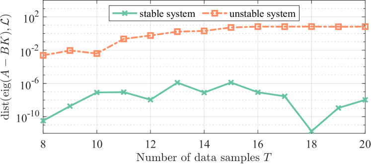
Figure 1: Simulations comparing the accuracy of the closed-loop pole locations when (8) is applied to open-loop data generated by a stable system (green line) and an unstable system (orange dashed line), for different values of the signal length $T$. Data for the unstable system has been generated by simulating the chemical reactor (VI), while the data for the stable system has been generated by a pre-stabilized reactor model. The simulation illustrates that (8) is more accurate by several orders of magnitude when applied to data generated by a stable system.

Next, we compare the accuracy of the closed-loop pole locations obtained using the data-based formula (8) with those obtained using a model-based pole placement formula, applied to an identified model. In both cases, the methods are applied to noisy data, and we conducted Montecarlo simulations by averaging over $100$ experiments. To this aim, we generated noisy data by simulating:

$$x(t+1)=A_{0}x(t)+B_{0}u(t)+e(t),$$

with $x(0)\sim\mathcal{N}(0,I_{n})$, $u(t)\sim\mathcal{N}(0,I_{m})$, $e(t)\sim\mathcal{N}(0,\sigma_{e}^{2}I_{n})$, and the matrices $A_{0}$ and $B_{0}$ have been chosen randomly and such that the modulus of all the eigenvalues of $A_{0}$ is inside the unit circle and $(A_{0},B_{0})$ is controllable, with $m=\lfloor n/2\rfloor$. We identified $(A_{0},B_{0})$ from noisy data by solving the least-squares problem:

$$\begin{bmatrix}A&B\end{bmatrix}\in\arg\min_{[A,B]}\|X_{1}-\begin{bmatrix}A&B\end{bmatrix}\begin{bmatrix}X_{0}\\ U_{0}\end{bmatrix}\|_{\text{F}}.$$

The set $\mathcal{L}$ has been chosen so that its entries are uniformly distributed in the real interval $[-n,n]$ and, for the model-based pole placement, we determined the feedback gain $K$ using the built-in place routine in Matlab R2022a. Fig. 2 compares the accuracy of the closed-loop pole locations obtained by using a model-based placement formula and the data-based formula (8) for increasing values of the state space size $n$. As illustrated by the figure, the pole locations obtained using the data-based formula (8) are more accurate by about one order of magnitude for all considered values of $n$. Moreover, by comparing the results for three different choices of the noise variance: $\sigma_{e}^{2}=1$ (top), $\sigma_{e}^{2}=10$ (middle), and $\sigma_{e}^{2}=100$ (bottom), the numerics suggest the higher the noise variance, the more the data-driven approach becomes preferable over the model-based one.

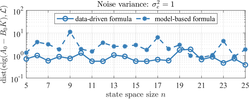
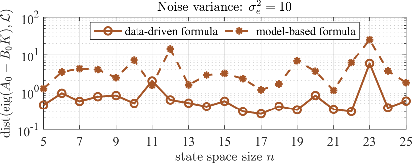
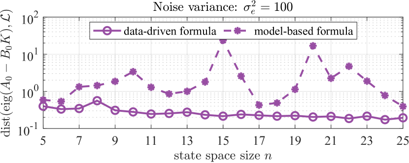
Figure 2: Montecarlo simulation comparing the accuracy of (8) when applied to noisy data with Gaussian distribution and three different levels of variance: $\sigma_{e}^{2}=1$ (top), $\sigma_{e}^{2}=10$ (middle), and $\sigma_{e}^{2}=100$ (bottom). The results suggest that the higher the noise variance, the more the data-driven formula becomes preferable over a model-based pole placement approach.

VII Conclusions

In this paper, we derived data-driven formulas to compute static feedback gains matrices that assign arbitrarily the eigenstructure of a linear dynamical system. By leveraging the linearity of the dynamics and a persistence of excitation condition, we showed for the first time that the closed-loop eigenstructure can be assigned exactly. Further, we illustrated the benefits of the data-driven methods, as compared to the model-based counterpart, through a set of numerical simulations, which showcase the numerical robustness of the approach, especially in the presence of noise in the measured data. This paper also opens several directions for future research, including an analytical investigation of the sensitivity of the closed-loop pole locations in the presence of noise in the data, and the extension to cases where the open-loop system contains uncontrollable modes.

References

- [1] V. Krishnan and F. Pasqualetti, “On direct vs indirect data-driven predictive control,” in IEEE Conf. on Decision and Control, Austin, TX, Dec. 2021, pp. 736–741.
- [2] F. Dörfler, J. Coulson, and I. Markovsky, “Bridging direct & indirect data-driven control formulations via regularizations and relaxations,” IEEE Transactions on Automatic Control, 2022, (Early access).
- [3] C. De Persis and P. Tesi, “Formulas for data-driven control: Stabilization, optimality, and robustness,” IEEE Transactions on Automatic Control, vol. 65, no. 3, pp. 909–924, 2019.
- [4] G. Baggio, V. Katewa, and F. Pasqualetti, “Data-driven minimum-energy controls for linear systems,” IEEE Control Systems Letters, vol. 3, no. 3, pp. 589–594, 2019.
- [5] J. Coulson, J. Lygeros, and F. Dörfler, “Data-enabled predictive control: In the shallows of the DeePC,” in European Control Conference, 2019, pp. 307–312.
- [6] T. M. Maupong and P. Rapisarda, “Data-driven control: A behavioral approach,” Systems & Control Letters, vol. 101, pp. 37–43, 2017.
- [7] S. Talebi, S. Alemzadeh, N. Rahimi, and M. Mesbahi, “Online regulation of unstable LTI systems from a single trajectory,” arXiv preprint, 2020, arXiv:2006.00125.
- [8] J. Berberich, J. Koehler, M. A. Müller, and F. Allgöwer, “Data-driven model predictive control with stability and robustness guarantees,” IEEE Transactions on Automatic Control, 2020, to appear.
- [9] L. Xu, M. Turan Sahin, B. Guo, and G. Ferrari-Trecate, “A data-driven convex programming approach to worst-case robust tracking controller design,” arXiv preprint, 2021, arXiv:2102.11918.
- [10] G. Bianchin, M. Vaquero, J. Cortés, and E. Dall’Anese, “Online stochastic optimization for unknown linear systems: Data-driven synthesis and controller analysis,” arXiv preprint, Aug. 2021, arXiv:2108.13040.
- [11] A. Allibhoy and J. Cortés, “Data-based receding horizon control of linear network systems,” IEEE Control Systems Letters, vol. 5, no. 4, pp. 1207–1212, 2020.
- [12] J. Berberich and F. Allgöwer, “A trajectory-based framework for data-driven system analysis and control,” in European Control Conference, 2020, pp. 1365–1370.
- [13] M. Guo, C. De Persis, and P. Tesi, “Data-driven stabilization of nonlinear polynomial systems with noisy data,” IEEE Transactions on Automatic Control, 2022, (early access) arXiv:2011.07833.
- [14] J. C. Willems, P. Rapisarda, I. Markovsky, and B. D. Moor, “A note on persistency of excitation,” Systems & Control Letters, vol. 54, no. 4, pp. 325–329, 2005.
- [15] A. Pandey, R. Schmid, and T. Nguyen, “Performance survey of minimum gain exact pole placement methods,” in European Control Conference, 2015, pp. 1808–1812.
- [16] J. Kautsky, N. K. Nichols, and P. Van Dooren, “Robust pole assignment in linear state feedback,” International Journal of control, vol. 41, no. 5, pp. 1129–1155, 1985.
- [17] S. P. Bhattacharyya and E. De Souza, “Pole assignment via Sylvester’s equation,” Systems & Control Letters, vol. 1, no. 4, pp. 261–263, 1982.
- [18] M. A. Rami, S. El Faiz, A. Benzaouia, and F. Tadeo, “Robust exact pole placement via an LMI-based algorithm,” IEEE Transactions on Automatic Control, vol. 54, no. 2, pp. 394–398, 2009.
- [19] S. Mukherjee and R. R. Hossain, “Data-driven pole placement in LMI regions with robustness guarantees,” in IEEE Conf. on Decision and Control, 2022, pp. 4010–4015.
- [20] C.-T. Chen, Linear System: Theory and Design. Holt, Rinehart, and Winston, 1984.
- [21] J. H. Wilkinson, The algebraic eigenvalue problem. London: Oxford University Press, 1988.