Unitarity of the SoV Transform for $\mathrm{SL}(2,\mathbb{C})$ Spin Chains

Unitarity of the SoV Transform
for $\boldsymbol{\mathrm{SL}(2,\mathbb{C})}$ Spin Chains

Alexander N. MANASHOV

A.N. Manashov

Max-Planck-Institut für Physik, Werner-Heisenberg-Institut, 80805 München, Germany alexander.manashov@desy.de

Received March 30, 2023, in final form October 20, 2023; Published online November 04, 2023

We prove the unitarity of the separation of variables transform for $\mathrm{SL}(2,\mathbb{C})$ spin chains by a method based on the use of Gustafson integrals.

spin chains; separation of variables; Gustafson’s integrals

33C70; 81R12

1 Introduction

Theory of quantum integrable models is an important part of modern theoretical physics. The solution of such models relies on the Quantum inverse scattering method (QISM) which includes such techniques as the algebraic Bethe ansatz (ABA) [50] and separation of variables (SoV) [48, 49]. The ABA allows one to effectively calculate energies and eigenstates of integrable models and to address more complicated problems such as calculating norms [32], scalar products [51] and correlation functions [28, 31]. Models with infinite-dimensional Hilbert spaces without a pseudo-vacuum state, the Toda chain [27] being the most famous example, are, however, beyond ABA’s grasp. The solution of such models relies on the SoV method proposed by Sklyanin [48, 49]. The method consists in constructing a map between the original Hilbert space, ${\mathbb{H}}_{\rm org}$, in which the model is formulated, and an auxiliary Hilbert space, ${\mathbb{H}}_{\rm SoV}$. This map is constructed in such a way that a multidimensional spectral problem associated with the original Hamiltonian is reduced to a one-dimensional problem on an auxiliary Hilbert space which usually takes the form of the Baxter $T$-$Q$ relation. Technically constructing the SoV representation is equivalent to finding the eigenfunctions of an element of the monodromy matrix associated with the model. For the Toda chain it was done by Kharchev and Lebedev [29, 30]. Later, a regular method for obtaining eigenfunctions for models with an $R$-matrix of the rank one was developed in [9], and at present the SoV representation is known for a number of models [2, 10, 11, 14, 47].

In order to be sure that the spectral problems in the original and auxiliary Hilbert spaces are equivalent, it is necessary to show that the corresponding map, ${\mathbb{H}}_{\rm SoV}\mapsto{\mathbb{H}}_{\rm org}$, is unitary (or that the eigenfunctions form a complete set in ${\mathbb{H}}_{\rm org}$). If $\dim{\mathbb{H}}_{\rm org}<\infty$ the problem can be solved, at least in principle, by counting the dimensions of the Hilbert spaces. For the models with infinite-dimensional Hilbert space, such as the Toda chain, the noncompact $\mathrm{SL}(2,\mathbb{C})$ spin chain, etc., the task becomes more difficult. For the Toda chain, unitarity was first established by using harmonic analysis of Lie groups techniques [46, 54]. However, this method is quite sophisticated and can hardly be generalized to more complicated cases. The rigorous proof of the unitarity of the SoV transform for the Toda chain based on the use of natural objects for the QISM was given by Kozlowski [33]. This technique was later applied to the modular $XXZ$ magnet [12]. Later it was realized [15] that there exists a close relation between $\mathrm{SL}(2,\mathbb{R})$ symmetric spin chains and the multidimensional Mellin–Barnes integrals studied by Gustafson [25, 26] that allowed to greatly simplify the proof of the unitarity of the SoV transform for $\mathrm{SL}(2,\mathbb{R})$ symmetric spin chains [13].

In the present paper, we apply this technique to the analysis of the noncompact spin chains with the $\mathrm{SL}(2,\mathbb{C})$ symmetry group. Such models appear in the studies of the Regge limit of scattering amplitudes in gauge theories, in QCD in particular [1, 19, 35, 36, 37], see also [4, 5, 6, 7] for recent developments. The SoV representation for the $\mathrm{SL}(2,\mathbb{C})$ spin chains was constructed in [9] while the generalization of Gustafson integrals relevant for the $\mathrm{SL}(2,\mathbb{C})$ spin chains was obtained recently in [16, 45]. Based on these results, we present below a proof of unitarity of the SoV transform for a generic $\mathrm{SL}(2,\mathbb{C})$ spin chain.

The paper is organized as follows. In Section 2, we recall elements of the QISM relevant for further analysis. The eigenfunctions of the elements of the monodromy matrix are constructed in Section 3. In Section 4, we calculate several scalar products of the eigenfunctions and discuss their properties. Section 5 contains the proof of unitarity of the SoV transform. Section 6 is reserved for a summary and several appendices contain a discussion of technical details.

2 $\boldsymbol{\mathrm{SL}(2,\mathbb{C})}$ spin chains

Spin chains are quantum mechanical systems whose dynamical variables are spin generators. We consider models with spin generators belonging to the unitary continuous principal series representation, $\mathrm{T}^{(s_{k},\bar{s}_{k})}$, of the unimodular group of complex two by two matrices. Namely, each site of the chain is equipped with two sets of generators, holomorphic ($S^{\alpha}$) and anti-holomorphic ones $\big{(}\bar{S}^{\alpha}\big{)}$,

$$S^{-}_{k}=-\partial_{z_{k}},\qquad S^{0}_{k}=z_{k}\partial_{z_{k}}+s_{k},\qquad S^{+}_{k}=z_{k}^{2}\partial_{z_{k}}+2s_{k}z_{k},$$

$$\bar{S}^{-}_{k}=-\partial_{\bar{z}_{k}},\qquad \bar{S}^{0}_{k}=\bar{z}_{k}\partial_{\bar{z}_{k}}+\bar{s}_{k},\qquad \bar{S}^{+}_{k}=\bar{z}_{k}^{2}\partial_{\bar{z}_{k}}+2\bar{s}_{k}\bar{z}_{k}.$$

The generators $S^{\alpha}_{k}\big{(}\bar{S}^{\alpha}_{k}\big{)}$ satisfy the standard $\mathfrak{sl}(2)$ commutation relations, while the generators at different sites and holomorphic and anti-holomorphic generators commute, $\big{[}S^{\alpha}_{k},\bar{S}^{\alpha^{\prime}}_{k}\big{]}=0$. The parameters $s_{k}$, $\bar{s}_{k}$ specifying the representation take the form [21]

$$s_{k}=\frac{1+n_{k}}{2}+{\rm i}\rho_{k},\qquad\bar{s}_{k}=\frac{1-n_{k}}{2}+{\rm i}\rho_{k},$$

where $n_{k}$ is an integer or half-integer number and $\rho_{k}$ is real, so that

$$s_{k}+\bar{s}_{k}^{*}=1\qquad\text{and}\qquad s_{k}-\bar{s}_{k}=n_{k}\in\mathbb{Z}/2.$$

The later condition comes from the requirement for the finite group transformations to be well defined while the former one guarantees the unitary character of transformations and anti-hermiticity of the generators, $\big{(}S_{k}^{\alpha}\big{)}^{\dagger}=-\bar{S}_{k}^{\alpha}$.

The Hilbert space of the model is given by the direct product of the Hilbert spaces at each node. For a chain of length $N$, ${\mathbb{H}}_{N}=\bigotimes_{k=1}^{N}\mathcal{H}_{k}$, where $\mathcal{H}_{k}=L_{2}(\mathbb{C})$.

In the QISM [34, 49, 50, 52], the dynamics of the model is determined by a family of mutually commuting operators. Namely, one defines the so-called $L$-operators,

$$L_{k}(u)=u+{\rm i}\begin{pmatrix}S_{k}^{0}&S_{k}^{-}\vspace{1mm}\\ S_{k}^{+}&-S_{0}^{-}\end{pmatrix},\qquad\bar{L}_{k}(\bar{u})=\bar{u}+{\rm i}\begin{pmatrix}\bar{S}_{k}^{0}&\bar{S}_{k}^{-}\vspace{1mm}\\ \bar{S}_{k}^{+}&-\bar{S}_{0}^{-}\end{pmatrix},$$

which are the basic building blocks in the QISM. The complex variables $u$, $\bar{u}$ are called spectral parameters. The next important object – a monodromy matrix – is given by the product of $L$ operators

$$T_{N}(u)=L_{1}(u+\xi_{1})L_{2}(u+\xi_{2})\cdots L_{N}(u+\xi_{N}),$$

$$\bar{T}_{N}(\bar{u})=\bar{L}_{1}\big{(}\bar{u}+\bar{\xi}_{1}\big{)}\bar{L}_{2}\big{(}\bar{u}+\bar{\xi}_{2}\big{)}\cdots\bar{L}_{N}\big{(}\bar{u}+\bar{\xi}_{N}\big{)},$$ (2.1)

where $\xi_{k}$, $\bar{\xi}_{k}$ are the so-called impurity parameters. The entries of the monodromy matrix,

$$T_{N}(u)=\begin{pmatrix}A_{N}(u)&B_{N}(u)\\ C_{N}(u)&D_{N}(u)\end{pmatrix},$$

are polynomials in $u$ with the operator valued coefficients, e.g.,

$$A_{N}(u)=u^{N}+u^{N-1}\big{(}{\rm i}S^{0}+\Xi\big{)}+\sum_{k=2}^{N}u^{N-k}a_{k},$$

$$B_{N}(u)=u^{N-1}{\rm i}S^{-}+\sum_{k=2}^{N}u^{N-k}b_{k},$$ (2.2)

where $\Xi=\sum_{k=1}^{N}\xi_{k}$ and $S^{0}$, $S^{-}$ are the total generators,

$$S^{\alpha}=S^{\alpha}_{1}+\cdots+S^{\alpha}_{N}.$$

The entries of the monodromy matrix form commuting operator families [18, 50]

$$[A_{N}(u),A_{N}(v)]=[B_{N}(u),B_{N}(v)]=[C_{N}(u),C_{N}(v)]=[D_{N}(u),D_{N}(v)]=0.$$

In particular, each entry commutes with the corresponding total generator, $S^{\alpha}$,

$$\big{[}S^{0},A_{N}(u)\big{]}=\big{[}S^{0},D_{N}(u)\big{]}=0\qquad\text{and}\qquad[S^{-},B_{N}(u)]=\big{[}S^{+},C_{N}(u)\big{]}=0.$$

The same equations hold for the anti-holomorphic operators $\bar{A}_{N}$, $\bar{B}_{N}$, $\bar{C}_{N}$, $\bar{D}_{N}$ and, of course, the holomorphic and anti-holomorphic operators commute. Moreover it can be checked that if the impurity parameters satisfy the constraint $\bar{\xi}_{k}=\xi_{k}^{*}$ for all $k$, the following relations between holomorphic and anti-holomorphic operators hold:

$$(A_{N}(u))^{\dagger}=\bar{A}_{N}(u^{*}),\qquad(B_{N}(u))^{\dagger}=\bar{B}_{N}(u^{*}),$$

etc. This ensures that the operators $a_{k}$ and $\bar{a}_{k}$ in the expansion of $A_{N}(u)$, (2.2), and $\bar{A}_{N}(u)$, are adjoint to each other $a_{k}^{\dagger}=\bar{a}_{k}$ ($b_{k}^{\dagger}=\bar{b}_{k}$ etc.).

The commutativity of the operators $A_{N}(u)$, $B_{N}(u)$, $C_{N}(u)$, $D_{N}(u)$ implies that the following families of self-adjoint operators:

$$\mathfrak{A}_{N}=\big{\{}{\rm i}S^{0},{\rm i}\bar{S}^{0},a_{k}+\bar{a}_{k},{\rm i}(a_{k}-\bar{a}_{k}),k=2,\dots,N\big{\}},$$

$$\mathfrak{B}_{N}=\big{\{}{\rm i}S^{-},{\rm i}\bar{S}^{-},b_{k}+\bar{b}_{k},{\rm i}(b_{k}-\bar{b}_{k}),k=2,\dots,N\big{\}},$$

(and similarly for others) are commutative and can be diagonalized simultaneously. The corresponding eigenfunctions provide a convenient basis – Sklyanin’s representation of Separated Variables (SoV) – for the analysis of spin chain models [49].

The operators $B_{N}$ and $C_{N}$, ($A_{N}$ and $D_{N}$) are related to each other by the inversion transformation, see [14] for detail, so it is sufficient to construct eigenfunctions for the operators $B_{N}$ and $A_{N}$. The eigenfunctions of $B_{N}$ for the homogeneous chain were constructed in [9] and later on for the operator $A_{N}$ [14]. Extending this approach to the inhomogeneous case is rather straightforward.

3 Eigenfunctions

In this section, we present explicit expressions for the eigenfunctions of the operators $B_{N}$ and $A_{N}$ for a generic inhomogeneous spin chain with impurities. We start with the operator $B_{N}$ where the construction follows the lines of [9] with minimal modifications.

3.1 $\boldsymbol{B_{N}}$ operator

Let $\Lambda_{n}$ be an integral (layer) operator which maps functions of $n-1$ variables into functions of $n$ variables and depends on the spectral parameters $x$, $\bar{x}$ and the complex vectors $\gamma$, $\bar{\gamma}$ of dimension $2n-2$

$$[\Lambda_{n}(x|\gamma)f](z_{1},\dots,z_{n})$$

$$\qquad{}=\idotsint\Lambda_{n}(x|\gamma)(z_{1},\dots,z_{n}|w_{1},\dots,w_{n-1})f(w_{1},\dots,w_{n-1})\prod_{k=1}^{n-1}{\rm d}^{2}w_{k}.$$ (3.1)

The kernel is given by the following expression:

$$\Lambda_{n}(x|\gamma)(z_{1},\dots,z_{n}|w_{1},\dots,w_{n-1})=\prod_{k=1}^{n-1}D_{\gamma_{2k-1}-{\rm i}x}(z_{k}-w_{k})D_{\gamma_{2k}+{\rm i}x}(z_{k+1}-w_{k}),$$

where the function $D_{\alpha}(z)$ (propagator) is defined as follows:

$$D_{\alpha}(z)\equiv D_{\alpha,\bar{\alpha}}(z,\bar{z})={z^{-\alpha}\bar{z}^{-\bar{\alpha}}}.$$ (3.2)

We will assume that the indices $\alpha$, $\bar{\alpha}$ satisfy the condition $[\alpha]\equiv\alpha-\bar{\alpha}\in\mathbb{Z}$ so that the propagator is a single-valued function on the complex plane. It implies that the parameters $\gamma_{k}$ and $x$ have the form

$$\gamma_{k}=\frac{1}{2}+\frac{r_{k}}{2}+{\rm i}\sigma_{k},\qquad\bar{\gamma}_{k}=\frac{1}{2}-\frac{r_{k}}{2}+{\rm i}\sigma_{k},\qquad x=\frac{{\rm i}m}{2}+\nu,\qquad\bar{x}=-\frac{{\rm i}m}{2}+\nu.$$ (3.3)

The numbers $\{m,r_{1},\dots,r_{2N-2}\}$ are either integer or half-integer and depending on this we call the corresponding variables integer (half-integer). The continuous parameters $\sigma_{k}$ and $\nu$ are subject to the constraints

$$\operatorname{Im}(\sigma_{2k+1}-\nu)>-\nicefrac{{1}}{{2}}\qquad\text{and}\qquad\operatorname{Im}(\sigma_{2k}+\nu)>-\nicefrac{{1}}{{2}},$$

which guarantee the convergence of the integral (3.1) for a smooth function $f$ with finite support. In the case we are most interested in, $\gamma_{k}+\bar{\gamma}_{k}=1$, the parameters $\sigma_{k}\in\mathbb{R}$, and the variable $\nu$ lies in the strip $-\nicefrac{{1}}{{2}}<\operatorname{Im}\nu<\nicefrac{{1}}{{2}}$.

The operators $\Lambda_{n}$ possess two important properties:

1. Let $\rho$ be a map which takes $M$-dimensional vectors

   $$\gamma=(\gamma_{1},\dots,\gamma_{M}),\qquad\bar{\gamma}=(\bar{\gamma}_{1},\dots,\bar{\gamma}_{M})$$

   to vectors of dimension $M-2$ as follows:

   $$\rho\gamma=(\gamma^{\prime}_{2},\gamma^{\prime}_{3},\dots,\gamma^{\prime}_{M-1}),\qquad\rho\bar{\gamma}=(\bar{\gamma}^{\prime}_{2},\bar{\gamma}^{\prime}_{3},\dots,\bar{\gamma}^{\prime}_{M-1}),$$

   where $a^{\prime}\equiv 1-a$. It can be shown that the operators $\Lambda_{n}$ and $\Lambda_{n-1}$ obey the following exchange relation:

   $$\Lambda_{n}(u|\gamma)\Lambda_{n-1}(v|\rho\gamma) =\omega_{n}(\gamma,u,v)\Lambda_{n}(v|\gamma)\Lambda_{n-1}(u|\rho\gamma).$$ (3.4)

   Here $\gamma(\bar{\gamma})$ is $(2n-2)$-dimensional vector and the factor $\omega_{n}$ is given by the following expression:

   $$\omega_{n}(\gamma,u,v) =\prod_{m=1}^{n-1}\boldsymbol{\Gamma}\left[\frac{\gamma_{2m-1}-{\rm i}v,\bar{\gamma}_{2m}+{\rm i}\bar{v}}{\gamma_{2m-1}-{\rm i}u,\bar{\gamma}_{2m}+{\rm i}\bar{u}}\right]=\prod_{m=1}^{n-1}\boldsymbol{\Gamma}\left[\frac{\bar{\gamma}_{2m-1}-{\rm i}\bar{v},\gamma_{2m}+{\rm i}v}{\bar{\gamma}_{2m-1}-{\rm i}\bar{u},\gamma_{2m}+{\rm i}u}\right],$$ (3.5)

   where

   $$\boldsymbol{\Gamma}\left[\frac{a_{1},a_{2},\dots,a_{n}}{b_{1},b_{2},\dots,b_{m}}\right]\equiv\frac{\prod_{k=1}^{n}\boldsymbol{\Gamma}[a_{k}]}{\boldsymbol{\prod}_{k=1}^{m}\boldsymbol{\Gamma}[b_{k}]}$$

   and $\boldsymbol{\Gamma}$ is the Gamma function of the complex field $\mathbb{C}$ [20]

   $$\boldsymbol{\Gamma}[u]\equiv\boldsymbol{\Gamma}[u,\bar{u}]={\Gamma(u)}/{\Gamma(1-\bar{u})}.$$

   The relation (3.4) is a direct consequence of the exchange relation for the propagators, see (A.1). Its proof is exactly the same as for the homogeneous spin chain. For more details, see [9, 14].

2. Let us choose the vector $\gamma$ as follows

   $$\gamma=(s_{1}-{\rm i}\xi_{1},s_{2}+{\rm i}\xi_{2},s_{2}-{\rm i}\xi_{2},\dots,s_{N-1}+{\rm i}\xi_{N-1},s_{N-1}-{\rm i}\xi_{N-1},s_{N}+{\rm i}\xi_{N}),$$

   $$\bar{\gamma}=(\bar{s}_{1}-{\rm i}\bar{\xi}_{1},\bar{s}_{2}+{\rm i}\bar{\xi}_{2},\bar{s}_{2}-{\rm i}\bar{\xi}_{2},\dots,\bar{s}_{N-1}+{\rm i}\bar{\xi}_{N-1},\bar{s}_{N-1}-{\rm i}\bar{\xi}_{N-1},\bar{s}_{N}+{\rm i}\bar{\xi}_{N}),$$ (3.6)

   where $s_{k}$ and $\xi_{k}$ are the spins and impurity parameters of the spin chain, respectively. For such a choice of the vector $\gamma$, the operator $B_{N}(x)$ annihilates $\Lambda_{N}(x|\gamma)$ [8, 9]

   $$B_{N}(x)\Lambda_{N}(x|\gamma)=0.$$ (3.7)

Let us define a function

$$\Psi^{(N)}_{p,x}(z) \equiv\Psi^{(N)}_{p,x_{1},\dots,x_{N-1}}(z_{1},\dots,z_{N})$$

$$=\pi^{-N^{2}/2}|p|^{N-1}\int{\rm d}^{2}zU_{x_{1},\dots,x_{N-1}}(z_{1},\dots,z_{N}|z){\rm e}^{{\rm i}(pz+\bar{p}\bar{z})},$$

where the kernel $U_{x_{1},\dots,x_{N-1}}$ is given by the product of the layer operators,

$$U_{x_{1},\dots,x_{N-1}}=\varpi(x|\gamma)\Lambda_{N}(x_{1}|\gamma)\Lambda_{N-1}(x_{2}|\rho\gamma)\Lambda_{N-2}\big{(}x_{3}|\rho^{2}\gamma\big{)}\cdots\Lambda_{2}\big{(}x_{N-1}|\rho^{N-2}\gamma\big{)},$$

and $\gamma$ is given by (3.6). Equation (3.4) guarantees that $U_{x_{1},\dots,x_{N-1}}\sim U_{x_{i_{1}},\dots,x_{i_{N-1}}}$ for any permutation of $x_{1},\dots,x_{N-1}$. The kernel $U_{x}$ becomes totally symmetric for the following choice of the prefactor $\varpi(x|\gamma)$:

$$\varpi({x}|\gamma) =\varpi(x_{1},\dots,x_{N-1}|\gamma)=\prod_{m=1}^{N-1}\prod_{k=1}^{m}\varpi_{1}\big{(}x_{k}|\rho^{m-1}\gamma\big{)},$$ (3.8)

where

$$\varpi_{1}(x|\gamma)=\varpi_{1}(x|\gamma_{1},\dots,\gamma_{2n})=\prod_{m=1}^{n}\boldsymbol{\Gamma}[\gamma_{2m-1}-{\rm i}x,\bar{\gamma}_{2m}+{\rm i}\bar{x}].$$

Thus the function $\Psi^{(N)}_{p,x_{1},\dots,x_{N-1}}$ is a symmetric function of the variables $x_{1},\dots,x_{N-1}$. Together with (3.7) it implies that

$$B_{N}(x_{k})\Psi^{(N)}_{p,x_{1},\dots,x_{N-1}}=0\qquad\text{for}\quad k=1,\dots,N-1.$$

Invariance of the kernel $U_{x_{1}m\dots,x_{N-1}}(z_{1},\dots,z_{N}|z)$ under shifts

$$U_{x_{1}\dots,x_{N-1}}(z_{1}+w,\dots,z_{N}+w|z+w)=U_{x_{1}\dots,x_{N-1}}(z_{1},\dots,z_{N}|z)$$

results in

$${\rm i}S^{-}\Psi^{(N)}_{p,x_{1},\dots,x_{N-1}}=p\Psi^{(N)}_{p,x_{1},\dots,x_{N-1}},\qquad{\rm i}\bar{S}^{-}\Psi^{(N)}_{p,x_{1},\dots,x_{N-1}}=\bar{p}\Psi^{(N)}_{p,x_{1},\dots,x_{N-1}}.$$ (3.9)

It follows then from equations (2.2), (3.7) and (3.9) that

$$B_{N}(u)\Psi^{(N)}_{p,x}(z)=p\prod_{k=1}^{N-1}(u-x_{k})\Psi^{(N)}_{p,x}(z),\qquad\bar{B}_{N}(\bar{u})\Psi^{(N)}_{p,x}(z)=\bar{p}\prod_{k=1}^{N-1}(\bar{u}-\bar{x}_{k})\Psi^{(N)}_{p,x}(z).$$

For $N=1$, the functions $\Psi_{p}^{(1)}(z,\bar{z})=\pi^{-1/2}{\rm e}^{{\rm i}(pz+\bar{p}\bar{z})}$ form the complete orthonormal system in ${\mathbb{H}}_{1}=L_{2}(\mathbb{C})$. The aim of this paper is to extend this statement to $N>1$. Namely, we will show in Section 5 that if the spins and impurities parameters of the spin chain obey the “unitarity” condition,

$$\gamma_{k}+\bar{\gamma}_{k}^{*}=1,$$ (3.10)

for all $k$ ($\gamma_{k}$ has the form (3.3) with $\sigma_{k}\in\mathbb{R}$ ) then the set of functions $\big{\{}\Psi^{(N)}_{p,x},x_{k}=\bar{x}_{k}^{*}(\nu_{k}\in\mathbb{R}),\allowbreak k=1,\dots,N-1\big{\}}$ is complete in ${\mathbb{H}}_{N}=(\bigotimes L_{2}(\mathbb{C}))^{N}$.

Note that the functions $\Psi_{p,x}^{(N)}$ are well defined for the complex parameters $\nu_{k}$ in the vicinity of the real line. For further analysis, it will be useful to consider regularized functions, $\Psi_{p,x}^{(N),\epsilon}$, by relaxing the last of the conditions (3.10) to $\gamma_{2N-2}+\bar{\gamma}_{2N-2}^{*}=1+2\epsilon$. This can be achieved by shifting the impurity parameter $\xi_{N}\to\xi_{N}-{\rm i}\epsilon$, i.e.,

$$\Psi_{p,x}^{(N),\epsilon}(z)\overset{\text{def}}{=}\Psi_{p,x}^{(N)}(z)\Big{|}_{\xi_{N}\to\xi_{N}-{\rm i}\epsilon}.$$ (3.11)

3.2 $\boldsymbol{A_{N}}$ operator

Construction of the eigenfunctions of the operator $A_{N}$ follows the scheme described in the previous subsection. We define a layer operator $\Lambda^{\prime}_{n}$ which maps functions of $n-1$ variables into functions of $n$ variables

$$[\Lambda^{\prime}_{n}(x|\gamma)f](z_{1},\dots,z_{n})$$

$$\qquad=\idotsint\Lambda^{\prime}_{n}(x|\gamma)(z_{1},\dots,z_{n}|w_{1},\dots,w_{n-1})f(w_{1},\dots,w_{n-1})\prod_{k=1}^{n-1}{\rm d}^{2}w_{k},$$

where the kernel is given by the following expression:

$$\Lambda^{\prime}_{n}(x|\gamma)(z_{1},\dots,z_{n}|w_{1},\dots,w_{n-1})$$

$$\qquad{}=D_{\gamma_{2n-1}-{\rm i}x}(z_{n})\prod_{k=1}^{n-1}D_{\gamma_{2k-1}-{\rm i}x}(z_{k}-w_{k})D_{\gamma_{2k}+{\rm i}x}(z_{k+1}-w_{k}).$$

The layer operator $\Lambda^{\prime}_{n}$ depends on the spectral parameters $x(\bar{x})$ and the vector $\gamma(\bar{\gamma})$ of dimension $2n-1$ which have the form (3.3). These operators satisfy the exchange relation

$$\Lambda^{\prime}_{n}(u|\gamma)\Lambda^{\prime}_{n-1}(v|\rho\gamma) =\omega_{n}(\gamma,u,v)\Lambda^{\prime}_{n}(v|\gamma)\Lambda^{\prime}_{n-1}(u|\rho\gamma),$$

and the factor $\omega_{n}$ is defined in (3.5).

Let $\Phi^{(N)}_{x}(z)$ be the following function:

$$\Phi^{(N)}_{x}(z)\equiv\Phi^{(N)}_{x_{1},\dots,x_{N}}(z_{1},\dots,z_{N})$$

$$\phantom{\Phi^{(N)}_{x}(z)}{}=\pi^{-N^{2}/2}\varpi(x|\gamma)\big{[}\Lambda^{\prime}_{N}(x_{1}|\gamma)\Lambda^{\prime}_{N-1}(x_{2}|\rho\gamma)\dots\Lambda^{\prime}_{1}\big{(}x_{N}|\rho^{N-1}\gamma\big{)}\big{]}(z_{1},\dots,z_{N}),$$

where $\gamma$ is $(2N-1)$-dimensional vector and the prefactor $\varpi$ is given by equation (3.8). For such a choice of $\varpi$ the function $\Phi^{(N)}_{x}$ is a symmetric function of the variables $x_{1},\dots,x_{N}$.

It can be shown that the operator $A_{N}(x)$ annihilates the layer operator $\Lambda^{\prime}_{N}(x|\gamma)$,

$$A_{N}(x)\Lambda^{\prime}_{N}(x|\gamma)=0,$$

for the following choice of the vector $\gamma$:

$$\gamma=(s_{1}-{\rm i}\xi_{1},s_{2}+{\rm i}\xi_{2},s_{2}-{\rm i}\xi_{2},\dots,s_{N}+{\rm i}\xi_{N},s_{N}-{\rm i}\xi_{N}),$$

$$\bar{\gamma}=(\bar{s}_{1}-{\rm i}\bar{\xi}_{1},\bar{s}_{2}+{\rm i}\bar{\xi}_{2},\bar{s}_{2}-{\rm i}\bar{\xi}_{2},\dots,\bar{s}_{N}+{\rm i}\bar{\xi}_{N},\bar{s}_{N}-{\rm i}\bar{\xi}_{N}).$$

Taking into account polynomiality of $A_{N}(u)$, see equation (2.2), one obtains

$$A_{N}(u)\Phi^{(N)}_{x}(z)=\prod_{k=1}^{N}(u-x_{k})\Phi^{(N)}_{x}(z),\qquad\bar{A}_{N}(\bar{u})\Phi^{(N)}_{x}(z)=\prod_{k=1}^{N}(\bar{u}-\bar{x}_{k})\Phi^{(N)}_{x}(z).$$

Again, the variables $x_{k}$, $\bar{x}_{k}$ are integers (half-integers) for all $k$. We will show that these functions, $\{\Phi^{(N)}_{x}(z),\,x_{k}=\bar{x}_{k}^{*},\,k=1,\dots,N\}$, form a complete set in the Hilbert space ${\mathbb{H}}_{N}$.

4 Scalar products, momentum representation, etc.

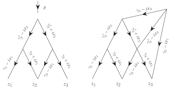
Figure 1: The diagrammatic representation for the function $\Psi$ (left) and $\Phi$ (right) for $N=3$. The arrow from $z$ to $w$ with an index $\alpha$ stands for the propagator $D_{\alpha}(z-w)$, equation (3.2).

The functions constructed in the previous section are given by multidimensional integrals. In this section, we show that these integrals converge for the parameters $\nu_{k}$ in the vicinity of real axis. To this end, it will be quite helpful, as was advocated in [9], to visualize the integrals as Feynman diagrams. The examples for $N=3$ are shown in Figure 1. It will be convenient to convert diagrams (functions) to momentum space

$$\Psi(z_{1},\dots,z_{N})={\pi^{-N}}\idotsint\widetilde{\Psi}(p_{1},\dots,p_{N}){\rm e}^{{\rm i}\sum_{k=1}^{N}(p_{k}z_{k}+\bar{p}_{k}\bar{z}_{k})}{\rm d}^{2}p_{1}\cdots{\rm d}^{2}p_{N}.$$

In momentum space the function $\Psi^{(N),\epsilon}_{p,x}$, equation (3.11), takes the form

$$\widetilde{\Psi}^{(N),\epsilon}_{p,x}(p_{1},\dots,p_{N})=\delta^{(2)}\left(p-\sum_{k=1}^{N}p_{k}\right)\Psi^{(N),\epsilon}_{x}(p_{1},\dots,p_{N}).$$

Let us remark here that the “$\epsilon$” regularization is reduced to a multiplication by the factor $(p_{N}\bar{p}_{N})^{\epsilon}$

$$\Psi^{(N),\epsilon}_{x}(p_{1},\dots,p_{N}) =(p_{N}\bar{p}_{N})^{\epsilon}\Psi^{(N)}_{x}(p_{1},\dots,p_{N}).$$ (4.1)

The function $\Psi^{(N),\epsilon}_{x}$ can be read from the Feynman diagram in Figure 1 as follows:

$$\Psi^{(N),\epsilon}_{x}(p_{1},\dots,p_{N})=\idotsint\mathcal{J}_{x}^{\epsilon}(\{p_{k}\},\{\ell_{ij}\})\prod_{1\leq j\leq i\leq N-2}{\rm d}^{2}\ell_{ij},$$ (4.2)

with the integrand $\mathcal{J}_{x}^{\epsilon}(\{p_{k}\},\{\ell_{ij}\})$ given by the product of the propagators, $D_{\alpha}(k)$. Up to a momentum independent factor

$$\mathcal{J}_{x}^{\epsilon}(\{p_{k}\},\{\ell_{ij}\})\simeq\prod_{k=1}^{N-1}\prod_{j=1}^{k}D_{\alpha_{kj}}(\ell_{k,j}-\ell_{k-1,j-1})D_{\beta_{kj}}(\ell_{k-1,j}-\ell_{k,j}),$$

where $\ell_{k0}\equiv 0$, $\ell_{k-1,k}\equiv p$ and $\ell_{N-1,j}=(p_{1}+\dots+p_{j})$. The indices $\alpha_{kj}$, $\beta_{kj}$ take the following values:

$$\alpha_{kj}=\gamma_{2j-1}^{(N-k)}+{\rm i}x_{N-k},\qquad\beta_{kj}=\gamma_{2j}^{(N-k)}-{\rm i}x_{N-k},$$

where we introduced the notations:

$$a^{(1)}=a^{\prime}=1-a\qquad\text{ and }\qquad a^{(k+1)}=1-a^{(k)}.$$

In many cases, Feynman diagrams can be evaluated diagrammatically. In particular, the computation of diagrams for the scalar product of $\Psi$ ($\Phi$) functions is based on the successive application of the exchange relation (A.1) to the diagram.

Let us consider the scalar product of two functions $\Psi^{(N),\epsilon}_{p,x}$ and $\Psi^{(N),\epsilon^{\prime}}_{q,y}$

$$\Big{(}\Psi^{(N),\epsilon^{\prime}}_{q,y},\Psi^{(N),\epsilon}_{p,x}\Big{)} =\pi\delta^{2}(p-q)(p\bar{p})^{\epsilon+\epsilon^{\prime}}I^{\epsilon,\epsilon^{\prime}}(x,y),$$ (4.3)

where

$$I^{\epsilon,\epsilon^{\prime}}(x,y) =\frac{1}{\pi}(p\bar{p})^{-\epsilon-\epsilon^{\prime}}\idotsint\delta^{(2)}\bigg{(}p-\sum_{k}p_{k}\bigg{)}\Psi^{(N),\epsilon}_{x}(\vec{p})\left(\Psi^{(N),\epsilon^{\prime}}_{y}(\vec{p})\right)^{\dagger}\prod_{j=1}^{N}{\rm d}^{2}p_{j}.$$ (4.4)

The function $I^{\epsilon,\epsilon^{\prime}}_{p}(x,y)$ is given by the Feynman diagram shown in Figure 2 in Appendix A (left panel), which is a multidimensional integral

$$I^{\epsilon,\epsilon^{\prime}}_{p}(x,y)=\idotsint\mathcal{I}^{\epsilon\epsilon^{\prime}}_{x,y}(p,\{\ell_{pr}\}|\gamma)\prod_{p,r=1}^{N-1}{\rm d}^{2}\ell_{pr}$$ (4.5)

with the integrand given by the product of the propagators. The diagram can be evaluated in a closed form by successively applying the exchange relation (A.1), that is equivalent to calculating the loop integrals in a certain order. The answer takes the form

$$I^{\epsilon,\epsilon^{\prime}}(x,y) =\mathscr{C}_{N}(\gamma)\boldsymbol{\Gamma}\left[\frac{\epsilon+\epsilon^{\prime}+{\rm i}X-{\rm i}\bar{Y}^{*}}{\epsilon+\epsilon^{\prime}}\right]\frac{\prod_{k,j=1}^{N-1}\boldsymbol{\Gamma}[{\rm i}(y_{k}^{*}-\bar{x}_{j})]}{\prod_{k=1}^{N-1}\bar{\phi}_{N}(\bar{x}_{k})(\phi_{N}(y_{k}))^{*}}$$

$$=\mathscr{C}_{N}(\gamma)\boldsymbol{\Gamma}\left[\frac{\epsilon+\epsilon^{\prime}+{\rm i}\bar{X}-{\rm i}Y^{*}}{\epsilon+\epsilon^{\prime}}\right]\frac{\prod_{k,j=1}^{N-1}\boldsymbol{\Gamma}[{\rm i}(\bar{y}_{k}^{*}-x_{j})]}{\prod_{k=1}^{N-1}\phi_{N}(x_{k})(\bar{\phi}_{N}(\bar{y}_{k}))^{*}},$$ (4.6)

where $X=\sum_{k=1}^{N-1}x_{k}$, $Y=\sum_{k=1}^{N-1}Y_{k}$ and

$$\phi_{N}(x)=\boldsymbol{\Gamma}\bigl{[}\gamma_{2N-3}-{\rm i}x,\gamma^{(1)}_{2N-4}-{\rm i}x,\gamma_{2N-5}-{\rm i}x,\dots,\gamma_{N}^{(N-3)}-{\rm i}x\bigr{]},$$

$$\bar{\phi}_{N}(\bar{x})=\boldsymbol{\Gamma}\bigl{[}\bar{\gamma}_{2N-3}-{\rm i}\bar{x},\bar{\gamma}^{(1)}_{2N-4}-{\rm i}\bar{x},\bar{\gamma}_{2N-5}-{\rm i}\bar{x},\dots,\bar{\gamma}_{N}^{(N-3)}-{\rm i}\bar{x}\bigr{]}.$$

For the sign factor $\mathscr{C}_{N}(\gamma)$, we get

$$\mathscr{C}_{N}(\gamma_{1},\gamma_{2},\dots,\gamma_{2N-2})=\begin{cases}1,&\text{odd }N,\\ (-1)^{\sum_{k=1}^{N-3}\bigl{[}\gamma_{2N-2-k}^{(k-1)}-\gamma_{N}^{(N-3)}\bigr{]}},&\text{even }N.\end{cases}$$ (4.7)

Here $[a]\equiv a-\bar{a}$. Details of the calculation can be found in Appendix B.

Let us show now that integrations in (4.5) can be done in an arbitrary order. The integrand in (4.5), $\mathcal{I}^{\epsilon\epsilon^{\prime}}_{x,y}(p,\{\ell_{pr}\}|\gamma)$, is given by the product of the propagators $D_{\alpha}(k)$, with each index being of the form $\alpha=\frac{1}{2}+\frac{n}{2}+{\rm i}\sigma$, momentum $k$ being a linear combination of loop momenta, $\ell_{ij}$, and the external momentum $p$. Since

$$\big{|}D_{\alpha}(k)\big{|}=\big{|}k^{-\alpha}\bar{k}^{-\bar{\alpha}}\big{|}=|k|^{-1+2\operatorname{Im}\sigma}=D_{\nicefrac{{1}}{{2}}-\operatorname{Im}\sigma}(k)$$

then for the parameters $\gamma$ satisfying the unitarity condition (3.10), and $x_{k}$, $y_{k}$ having the form

$$x_{k}={{\rm i}n_{k}}/{2}+\nu_{k},\qquad y_{k}={{\rm i}m_{k}}/{2}+\mu_{k},$$ (4.8)

one obtains for the modulus of the integrand

$$\big{|}\mathcal{I}^{\epsilon\epsilon^{\prime}}_{x,y}(p,\{\ell_{pr}\}|\gamma)\big{|}=\mathcal{I}^{\epsilon\epsilon^{\prime}}_{\underline{x},\underline{y}}(p,\{\ell_{pr}\}|\underline{\gamma})>0,$$

where the underlined variables are: $\underline{\gamma}=(\nicefrac{{1}}{{2}},\dots,\nicefrac{{1}}{{2}})$,

$$(\underline{x})_{k}=\operatorname{Im}(\nu_{k})=\epsilon_{k},\qquad(\underline{y})_{k}=\operatorname{Im}(\mu_{k})=\epsilon^{\prime}_{k}.$$

Thus the integral of $|\mathcal{I}^{\epsilon\epsilon^{\prime}}_{x,y}(p,\{\ell_{pr}\}|\gamma)|$ is a particular case of the integral (4.5) which was calculated by performing loop integrations in a certain order. Since all integrals converge under the conditions

$$\epsilon_{kj}\equiv\epsilon_{k}+\epsilon^{\prime}_{j}>0\qquad\text{for}\quad k,j=1,\dots,N-1\qquad\text{and}\qquad\epsilon+\epsilon^{\prime}>\sum_{k=1}^{N-1}(\epsilon_{k}+\epsilon^{\prime}_{k}),$$

by Fubini theorem, the integral (4.5) exists and the integrations can be done in an arbitrary order.

The following statements can immediately be deduced from this result:

• For any bounded function $\varphi(p,x)$ with a finite support the function

  $$\Psi^{\epsilon}_{\varphi}=\idotsint\varphi(p,x)\Psi^{(N),\epsilon}_{p,x^{\epsilon}}{\rm d}^{2}p\mathcal{D}x_{1}\cdots\mathcal{D}x_{N-1},$$ (4.9)

  where $x^{\epsilon}=(x_{1}+{\rm i}\epsilon_{1},\dots,x_{N-1}+{\rm i}\epsilon_{N-1})$, $x_{k}={\rm i}n_{k}/2+\nu_{k}$, $\epsilon_{k}>0$, $\epsilon>\sum_{k=1}^{N-1}\epsilon_{k}$ and

  $$\int\mathcal{D}x_{k}\equiv\sum_{n_{k}=-\infty}^{\infty}\int_{-\infty}^{\infty}{\rm d}\nu_{k},$$

  belongs to the Hilbert space ${\mathbb{H}}_{N}$, $\|\Psi^{\epsilon}_{\varphi}\|^{2}<\infty$, for sufficiently small $\epsilon$.

• It follows from the finiteness of the integral $I^{\epsilon,\epsilon^{\prime}}_{p}(x,y)$, equation (4.4), that the function $\Psi_{x}^{(N),\epsilon}(\vec{p})$, equation (4.2), exists almost for all $\vec{p}$ for the separated variables $x_{k}$ close to the real axis:

  $$\operatorname{Im}\nu_{k}=\frac{1}{2}\operatorname{Im}(x_{k}+\bar{x}_{k})\sim 0\qquad\text{for all $k$}$$

  and $\Psi_{x}^{(N),\epsilon}(\vec{p})$ is a continuous function of $\nu_{k}$ in this region. Indeed, let us fix $m<N$ and put $u_{m}=\text{Re}\nu_{m}$ and $v_{m}=\operatorname{Im}\nu_{m}$, $|v_{m}|<\delta$. One gets the following estimate for the integrand (4.5):

  $$|\mathcal{J}_{x}^{\epsilon}(\{p_{k}\},\{\ell_{ij}\})|<|\mathcal{J}_{x_{+}}^{\epsilon}(\{p_{k}\},\{\ell_{ij}\})|+|\mathcal{J}_{x_{-}}^{\epsilon}(\{p_{k}\},\{\ell_{ij}\})|,$$ (4.10)

  where $x_{\pm}$ are defined as follows: for $k\neq m$ $(x_{\pm})_{k}=x_{k}$ and for $k=m$ $(x_{\pm})_{m}=u_{m}\pm i\delta$. The integrals of the functions on the right-hand side of (4.10) are finite for sufficiently small $\delta$. It follows then from the Lebesgue theorem that the function $\Psi_{x}^{(N),\epsilon}(\vec{p})$ is continuous in the variable $\nu_{m}$.

The scalar product of the functions $\Psi^{(N)}_{p,y}$ and $\Phi^{(N)}_{x}$ constructed in Section 3.2 can be calculated in a similar way. Note that there is no need to introduce “$\epsilon$” regulator here. The corresponding integral is absolutely convergent when $\operatorname{Im}(\nu_{k}+\mu_{j})>0$ for all $k$, $j$ ($x_{k}$, $y_{j}$ given by (4.8)). The scalar product takes the form

$$\big{(}\Psi^{(N)}_{p,y}|\Phi^{(N)}_{x}\big{)}={} \mathrm{C}^{AB}_{N}(\gamma)|p|^{N-1}(-{\rm i}p)^{-G_{N}-{\rm i}X}({\rm i}\bar{p})^{-\bar{G}_{N}-{\rm i}\bar{X}}$$

$$\times\frac{\prod_{k=1}^{N}\prod_{j=1}^{N-1}\boldsymbol{\Gamma}[{\rm i}(\bar{y}_{j}^{*}-x_{k})]}{\left(\prod_{j=1}^{N}\vartheta_{N}(x_{j})\right)\left(\prod_{j=1}^{N-1}\bar{\vartheta}_{N}(\bar{y}_{j})\right)^{\dagger}},$$ (4.11)

where

$$\vartheta_{N}(x)=\prod_{k=1}^{N}\boldsymbol{\Gamma}\bigl{[}\gamma^{(k-1)}_{2N-k}-{\rm i}x_{j}\bigr{]},\qquad\bar{\vartheta}_{N}(\bar{x})=\prod_{k=1}^{N}\boldsymbol{\Gamma}\bigl{[}\bar{\gamma}^{(k-1)}_{2N-k}-{\rm i}\bar{x}_{j}\bigr{]},$$

$G_{N}=\sum_{k=N}^{2N-1}\gamma_{k}^{(k)}$, $X=\sum_{k=1}^{N}x_{k}$ and

$$\mathrm{C}^{AB}_{N}(\gamma_{1},\dots,\gamma_{2N-1})=\begin{cases}1,&\text{odd }N,\\ (-1)^{\sum_{k=1}^{N}\bigl{[}\gamma_{2N-k}^{(k-1)}-\gamma_{N}^{(N-1)}\bigr{]}},&\text{even }N.\end{cases}$$

Similar to the previous case one can argue that $\Phi^{(N)}_{x}$ is a continuous function of $\nu_{k}$ in the vicinity of the real axis.

Finally, the scalar product of the functions $\Psi^{(N+1)}_{p,x}(z_{1},\dots,z_{N+1})$ and $\Psi^{(N)}_{q_{1},y}(z_{1},\dots,z_{N})\otimes\Psi^{(1)}_{q_{2}}(z_{N+1})$ which we need in the proof of Theorem 5.2, takes the form

$$\big{(}\Psi^{N}_{q_{1},y}\otimes\Psi^{(1)}_{q_{2}},\Psi^{(N+1)}_{p,x}\big{)}=\mathrm{C}_{NN+1}(\gamma)\pi\delta^{(2)}(p-q_{1}-q_{2})|p|^{N}|q_{1}|^{N-1}$$

$$\qquad\times({\rm i}p)^{-\bar{G}_{N+1}^{*}}(-{\rm i}\bar{p})^{-G_{N+1}^{*}}({\rm i}q_{2})^{-\gamma^{\prime}_{2N}}(-{\rm i}\bar{q}_{2})^{-\bar{\gamma}^{\prime}_{2N}}(-{\rm i}q_{1})^{-G_{N}}({\rm i}\bar{q}_{1})^{-\bar{G}_{N}}$$

$$\qquad\times\left(1+\frac{q_{1}}{q_{2}}\right)^{{\rm i}\bar{Y}^{*}}\left(1+\frac{\bar{q}_{1}}{\bar{q}_{2}}\right)^{{\rm i}Y^{*}}\left(-\frac{q_{2}}{q_{1}}\right)^{iX}\left(-\frac{\bar{q}_{2}}{\bar{q}_{1}}\right)^{i\bar{X}}$$

$$\qquad\times\frac{\prod_{k=1}^{N-1}\prod_{j=1}^{N}\boldsymbol{\Gamma}\left[{\rm i}(\bar{y}_{k}^{*}-x_{j})\right]}{\left(\prod_{j=1}^{N}\prod_{k=1}^{N-1}\boldsymbol{\Gamma}\bigl{[}\gamma_{2N-k}^{(k-1)}-{\rm i}x_{j}\bigr{]}\right)\left(\prod_{k=1}^{N}\prod_{j=1}^{N-1}\boldsymbol{\Gamma}\bigl{[}\bar{\gamma}_{2N-k}^{(k-1)}-{\rm i}\bar{y}_{j}\bigr{]}\right)^{\dagger}},$$ (4.12)

where

$$G_{N}=\sum_{m=N}^{2N-1}\gamma_{m}^{(m)},\qquad G_{N+1}=G_{N}-\gamma_{N}^{(N)}=\sum_{m=N+1}^{2N-1}\gamma_{m}^{(m)}$$ (4.13)

and

$$\mathrm{C}_{NN+1}(\gamma_{1},\dots,\gamma_{2N})=\begin{cases}1,&\text{for odd}\ N,\\ (-1)^{\sum_{k=1}^{N-1}\bigl{[}\gamma_{2N-k}^{(k-1)}-\gamma_{N}^{(N-1)}\bigr{]}},&\text{for even}\ N.\end{cases}$$

The calculation is almost the same as in the previous cases so we omit the details.

5 SoV representation

In the previous section, we constructed the functions $\Psi_{p,x}^{(N)}$ and $\Phi^{(N)}_{x}$ associated with the entries $B_{N}$ and $A_{N}$ of the monodromy matrix (2.1). For a given vector $\Psi\in{\mathbb{H}}_{N}$, we define two functions by projecting it on $\Psi_{p,x}^{(N)}$ and $\Phi^{(N)}_{x}$:

$$\varphi(p,x_{1},\dots,x_{N-1})=\big{(}\Psi_{p,x}^{(N)},\Psi\big{)},\qquad\chi(x_{1},\dots,x_{N})=\big{(}\Phi_{x}^{(N)},\Psi\big{)}.$$

These functions are symmetric functions of the variables $x$. It was shown by Sklyanin [49] that the transformation $\Psi\mapsto\varphi(\Psi\mapsto\chi)$ reduces the original multidimensional spectral problem for the transfer matrix to the set of one-dimensional spectral problems that greatly simplifies the analysis. We want to show that the maps $\Psi\mapsto\varphi$ and $\Psi\mapsto\chi$ can be extended to the isomorphism between the Hilbert spaces, ${\mathbb{H}}_{N}\mapsto\mathbb{H}_{{\rm SoV}}$.

Let us define

$$\left(\varphi_{1},\varphi_{2}\right)_{B_{N}}=\int_{\mathbb{R}\times\mathbb{R}}\int_{\mathscr{D}^{\sigma}_{N-1}}(\varphi_{1}(p,x))^{\dagger}\varphi_{2}(p,x)\mu_{N-1}\left(x\right){\rm d}^{2}p{\rm d}\mu^{B}_{N-1}(x),$$

$$\left(\chi_{1},\chi_{2}\right)_{A_{N}}=\int_{\mathscr{D}^{\sigma}_{N}}(\chi_{1}(x))^{\dagger}\chi_{2}(x){\rm d}\mu^{A}_{N}(x).$$ (5.1)

The variables $x_{k}$, $\bar{x}_{k}$ take the form $x_{k}={\rm i}n_{k}/2+\nu_{k}$, $\bar{x}_{k}=-{\rm i}n_{k}/2+\nu_{k}$, where all $n_{k}$ are either integers or half-integers,

$$n_{k}\in\mathbb{Z}^{\sigma}\equiv\mathbb{Z}+\frac{\sigma}{2},\qquad\sigma=0,1,$$

and

$$\mathscr{D}^{\sigma}_{N}\equiv\left(\mathbb{R}\times Z^{\sigma}\right)^{N}.$$

The measures are defined as follows:

$$d\mu^{B(A)}_{N}(x)=\mu^{B(A)}_{N}(x)\prod_{k=1}^{N}\mathcal{D}x_{k},\qquad\mu^{B(A)}_{N}(x)=c_{N}^{B(A)}\mu_{N}(x).$$

The symbol $\mathcal{D}x$ stands for

$$\int\mathcal{D}x\equiv\sum_{n\in\mathbb{Z}^{\sigma}}\int_{-\infty}^{\infty}{\rm d}\nu.$$

The weight function $\mu_{N}(x)$ is given by the following expression:

$$\mu_{N}(x_{1},\dots,x_{N}) =\prod_{1\leq k<j\leq N}x_{kj}\bar{x}_{kj}=\prod_{1\leq k<j\leq N}\left(\nu_{kj}^{2}+\frac{1}{4}n_{kj}^{2}\right),$$

where $x_{kj}=x_{k}-x_{j}$, $\nu_{kj}=\nu_{k}-\nu_{j}$, $n_{kj}=n_{k}-n_{j}$ while the coefficients $c_{N}^{B(A)}$ take the form

$$\left(c_{N}^{B}\right)^{-1}=\frac{1}{2}{(2\pi)^{N+1}N!},\qquad\left(c_{N}^{A}\right)^{-1}={(2\pi)^{N}N!}.$$

Let ${\mathbb{H}}_{N}^{B,\sigma}$, ${\mathbb{H}}_{N}^{A,\sigma}$ be the Hilbert spaces of symmetric functions corresponding to the scalar products (5.1):

$${\mathbb{H}}_{N}^{B,\sigma}=L^{2}(\mathbb{R}\times\mathbb{R})\otimes L^{2}_{\mathrm{sym}}\left(\mathscr{D}^{\sigma}_{N-1},{\rm d}\mu^{B}_{N-1}(x)\right),$$

$${\mathbb{H}}_{N}^{A,\sigma}=L^{2}_{\mathrm{sym}}\left(\mathscr{D}^{\sigma}_{N},{\rm d}\mu^{A}_{N}(x)\right).$$

Given that $\varphi(p,x)$ and $\chi(x)$ are smooth and compactly supported functions on $\mathbb{R}^{2}\times\mathscr{D}^{\sigma}_{N-1}$ and $\mathscr{D}^{\sigma}_{N}$, respectively, we introduce transforms $\mathrm{T}_{N}^{B}\colon\varphi\mapsto\Psi_{\varphi}$ and $\mathrm{T}_{N}^{A}\colon\chi\mapsto\Psi_{\chi}$,

$$\Psi_{\varphi}(z)\equiv\big{[}\mathrm{T}_{N}^{B}\varphi\big{]}(z)=\int_{\mathbb{R}^{2}}\int_{\mathscr{D}^{\sigma}_{N-1}}\varphi(p,x)\Psi_{p,x}^{(N)}(z){\rm d}^{2}p{\rm d}\mu^{B}_{N-1}(x),$$ (5.2a)

$$\Phi_{\chi}(z)\equiv\big{[}\mathrm{T}_{N}^{A}\chi\big{]}(z)=\int_{\mathscr{D}^{\sigma}_{N}}\chi(x)\Phi_{p,x}^{(N)}(z){\rm d}\mu^{A}_{N}(x).$$ (5.2b)

Note that the function $\Psi_{\varphi}$ depends on the vector $\gamma$, equation (3.6), which appears in the definition of the function $\Psi_{p,x}^{(N)}$. That is $\mathrm{T}_{N}^{B}\equiv\mathrm{T}_{N}^{B}(\gamma)$ and the same applies to the operator $\mathrm{T}_{N}^{A}$. In order to not overload the notation, we do not display this dependence explicitly.

5.1 $\boldsymbol{B}$ system

We begin the proof of the unitarity of the transform $\mathrm{T}_{N}^{B}$ with the following lemma.

Lemma 5.1.

For any smooth fast decreasing function $\varphi$ on $\mathbb{R}^{2}\times\mathscr{D}^{\sigma}_{N-1}$, the function $\mathrm{T}_{N}^{B}\varphi$ belongs to the Hilbert space ${\mathbb{H}}_{N}$ and it holds

$$\big{\|}\mathrm{T}_{N}^{B}\varphi\big{\|}_{{\mathbb{H}}_{N}}^{2}=\|{\varphi}\|_{{\mathbb{H}}_{N}^{B,\pm}}^{2}=\int_{\mathfrak{D}_{N}^{\pm}}|\varphi(p,x)|^{2}{\rm d}^{2}p{\rm d}\mu_{N-1}^{B}(x).$$

Proof.

Let $\Psi_{\varphi}^{\epsilon}$ be a function defined by equation (5.2a) with $\Psi_{p,x}^{(N)}$ replaced by $\Psi_{p,x^{\epsilon}}^{(N),\epsilon}$, see equations (4.1) and (4.9). It can be shown that $\Psi_{\varphi}^{\epsilon}(\vec{p})\underset{\epsilon\to 0}{\mapsto}\Psi_{\varphi}(\vec{p})$ almost everywhere. Next, taking into account equation (4.3) one gets

$$(\Psi_{\varphi}^{\epsilon},\Psi_{\varphi^{\prime}}^{\epsilon^{\prime}})_{{\mathbb{H}}_{N}}={} \pi\int{\rm d}^{2}p\int{\rm d}\mu_{N-1}^{B}(x)$$

$$\times\int{\rm d}\mu_{N-1}^{B}(x^{\prime})(p\bar{p})^{\epsilon+\epsilon^{\prime}}\varphi(p,x)(\varphi^{\prime}(p,x^{\prime}))^{\dagger}I^{\epsilon,\epsilon^{\prime}}(x,x^{\prime}),$$ (5.3)

with $I^{\epsilon,\epsilon^{\prime}}(x,x^{\prime})$ given by equation (4.6). Let us assume that the function $\varphi(\varphi^{\prime})$ has the form

$$\varphi(p,x_{1},\dots,x_{N-1})=\kappa(p)\phi(x_{1},\dots,x_{N-1}),$$ (5.4)

where $\phi(x_{1},\dots,x_{N-1})$ is a symmetric function

$$\phi(x_{1},\dots,x_{N-1})=\sum_{S_{N-1}}\phi_{1}(x_{i_{1}})\cdots\phi_{N-1}(x_{i_{N-1}})$$ (5.5)

and the sum goes over all permutations. We also assume that the functions $\phi_{k}(x_{k})=\phi_{k}(n_{k},\nu_{k})$ are local in $n_{k}$, $\phi(n_{k},\nu_{k})=\delta_{n_{k},m_{k}}\phi_{k}(\nu_{k})$ and $\phi_{k}(\nu_{k})$ is an analytic function of $\nu_{k}$ in some strip $|\operatorname{Im}\nu_{k}|<\delta_{k}$ which vanishes sufficiently fast at $\nu_{k}\to\pm\infty$. Such functions form a dense subspace in the Hilbert space ${\mathbb{H}}_{N}^{B,\sigma}$. Since the momentum integral in (5.3) factorizes one has to consider the integrals over $x_{k}=(n_{k},\nu_{k})$, $x^{\prime}_{k}=(n^{\prime}_{k},\nu^{\prime}_{k})$, which have the form

$$\int{\rm d}\mu_{N-1}^{B}(x)\int{\rm d}\mu_{N-1}^{B}(x^{\prime})\cdots$$

$$\qquad{}\equiv\prod_{j=1}^{N-1}\sum_{n_{j}\in\mathbb{Z}+\frac{\sigma}{2}}\sum_{n^{\prime}_{j}\in\mathbb{Z}+\frac{\sigma}{2}}\int_{-\infty}^{\infty}\cdots\int_{-\infty}^{\infty}\mu_{N-1}^{B}(\vec{n},\vec{\nu})\mu_{N-1}^{B}(\vec{n}^{\prime},\vec{\nu}^{\prime})\prod_{k=1}^{N-1}{\rm d}\nu_{k}{\rm d}\nu^{\prime}_{k}\cdots.$$ (5.6)

According to our assumptions, only finite number of terms contribute to the sum in (5.6). Let us study behaviour of a particular term in the sum in the limit $\epsilon,\epsilon^{\prime}\mapsto 0$. The functions $\phi$, $\phi^{\prime}$ are smooth and fast decreasing functions of $\nu$, $\nu^{\prime}$. The function $I^{\epsilon,\epsilon^{\prime}}(x,x^{\prime})$ contains the factor $\boldsymbol{\Gamma}[\epsilon+\epsilon^{\prime}+{\rm i}\bar{X}-{\rm i}(X^{\prime})^{*}]/\boldsymbol{\Gamma}[\epsilon+\epsilon^{\prime}]$ and the product of the $\boldsymbol{\Gamma}$-functions

$$\boldsymbol{\Gamma}\left[{\rm i}((\bar{x}^{\prime}_{k})^{*}-x_{j})\right] =\boldsymbol{\Gamma}\left[\frac{n^{\prime}_{k}}{2}-\frac{n_{j}}{2}+{\rm i}(\nu^{\prime}_{k}-\nu_{j})+\epsilon_{jk}\right]$$

$$=\frac{\Gamma\bigl{(}\frac{n^{\prime}_{k}}{2}-\frac{n_{j}}{2}+{\rm i}(\nu^{\prime}_{k}-\nu_{j})+\epsilon_{jk}\bigr{)}}{\Gamma\bigl{(}1+\frac{n^{\prime}_{k}}{2}-\frac{n_{j}}{2}-{\rm i}(\nu^{\prime}_{k}-\nu_{j})-\epsilon_{jk}\bigr{)}},$$ (5.7)

where $\epsilon_{jk}\equiv\epsilon_{j}+\epsilon^{\prime}_{k}$. In the $\epsilon^{\prime}_{k},\epsilon_{j}\to 0$ this function becomes singular at $\nu^{\prime}_{k}=\nu_{j}$ if $n^{\prime}_{k}=n_{j}$. Let us shift the contours of integrations over $\nu^{\prime}_{k}$ variables to the upper half-plane, $\operatorname{Im}\nu^{\prime}_{k}=\delta>\epsilon_{jk}$, and pick up the residues at the corresponding poles. After this, we can send $\epsilon^{\prime}_{k},\epsilon_{j}\mapsto 0$. Let us consider a generic contribution arising after this rearrangement. It has the form

$$\int_{C_{\delta}}\cdots\int_{C_{\delta}}\prod_{k=1}^{M}{\rm d}\nu^{\prime}_{i_{k}}f\left(x_{1},\dots,x_{N-1},S(x^{\prime}_{1}),\dots,S(x^{\prime}_{N-1})\right),$$

where $S(x^{\prime}_{k})=x^{\prime}_{k}$ if $k\in(i_{1},\dots,i_{M})$ and $S(x^{\prime}_{k})=x_{p_{k}}$ if $k$ does not belong to this set. The integrand $f$ is given by the product of the functions $\phi_{k}$, $\phi^{\prime}_{k}$, $\boldsymbol{\Gamma}$-functions (5.1) and the factor ${A=\boldsymbol{\Gamma}[\epsilon+\epsilon^{\prime}+{\rm i}\bar{X}-{\rm i}(X^{\prime})^{*}]/\boldsymbol{\Gamma}[\epsilon+\epsilon^{\prime}]}$. All these factors are regular on the contours of integration. Moreover, if $M\geq 1$ the last factor, $A$, tends to zero at $\epsilon,\epsilon^{\prime}\mapsto 0$. Thus the only non-vanishing contribution comes from the term with $M=0$, i.e., when all $x^{\prime}_{k}\mapsto x_{i_{k}}$ for $k=1,\dots,N-1$. It takes the form

$$(\Psi_{\varphi}^{\epsilon},\Psi_{\varphi^{\prime}}^{\epsilon^{\prime}})_{{\mathbb{H}}_{N}}=\int{\rm d}^{2}p\int{\rm d}\mu_{N-1}^{B}(x)\varphi(p,x)(\varphi^{\prime}(p,x))^{\dagger}+O(\epsilon+\epsilon^{\prime})$$

that results in the following estimate for the norm of the function $\Psi^{\epsilon}_{\varphi}$:

$$\|\Psi^{\epsilon}_{\varphi}\|^{2}_{{\mathbb{H}}_{N}}=K+O(\epsilon),$$

where

$$K=\|{\varphi}\|_{{\mathbb{H}}_{N}^{B,\sigma}}^{2}\equiv\int_{\mathbb{R}^{2}}\int_{\mathscr{D}^{\sigma}_{N-1}}|\varphi(p,x)|^{2}{\rm d}^{2}p{\rm d}\mu_{N-1}^{B}(x).$$

Since $\Psi_{\varphi}^{\epsilon}(\vec{p})\mapsto\Psi_{\varphi}(\vec{p})$ at $\epsilon\to 0$, it follows from Fatou’s theorem that $\|\Psi_{\varphi}\|^{2}_{{\mathbb{H}}_{N}}<K$. At the same time, the inequality

$$\|\Psi_{\varphi}-\Psi_{\varphi}^{\epsilon}\|^{2}_{{\mathbb{H}}_{N}}\geq 0$$

implies $\|\Psi_{\varphi}\|^{2}_{{\mathbb{H}}_{N}}\geq K$ that results in $\|\Psi_{\varphi}\|^{2}_{{\mathbb{H}}_{N}}=K$.

Since the set of functions (5.4), (5.5) is dense in the Hilbert spaces ${\mathbb{H}}_{N}^{B\pm}$, the transformation $\mathrm{T}_{N}^{B}$ can be extended to the entire Hilbert space ${\mathbb{H}}_{N}^{B,\pm}$ and equation (5.8a) holds for any function $\varphi\in\mathbb{H}_{N}^{B,\pm}$. ∎

Taking this result into account we formulate the following theorem.

Theorem 5.2.

The map $\mathrm{T}_{N}^{B}$ defined in equation (5.2a) can be extended to the linear bijective isometry of the Hilbert spaces, $\mathbb{H}_{N}^{B,\sigma}\mapsto\mathbb{H}_{N}$, i.e.,

$$\big{\|}\mathrm{T}_{N}^{B}\varphi\big{\|}_{{\mathbb{H}}_{N}}^{2} =\|{\varphi}\|_{{\mathbb{H}}_{N}^{B,\sigma}}^{2}$$ (5.8a)

and

$$\mathcal{R}\left(\mathrm{T}_{N}^{B}\right) ={\mathbb{H}}_{N}.$$ (5.8b)

Proof.

Equation (5.8a) is a direct consequence of Lemma 5.1. It implies that $\big{\|}\mathrm{T}_{N}^{B}\big{\|}=1$, hence $\mathcal{R}\big{(}\mathrm{T}_{N}^{B}\big{)}$ is a closed subspace in ${\mathbb{H}}_{N}$ and ${\mathbb{H}}_{N}=\mathcal{R}\big{(}\mathrm{T}_{N}^{B}\big{)}\oplus\mathcal{R}\big{(}\mathrm{T}_{N}^{B}\big{)}^{\perp}$. Since $\mathcal{R}\big{(}\mathrm{T}_{N}^{B}\big{)}^{\perp}=\ker\big{(}\mathrm{T}_{N}^{B}\big{)}^{*}$ in order to prove (5.8b) it is enough to show that $\ker\big{(}\mathrm{T}_{N}^{B}\big{)}^{*}=0$. ∎

We prove this statement using induction on $N$. For $N=1$, the map $\mathrm{T}_{N=1}^{B}$ is a two-dimensional Fourier transform, hence equation (5.8b) is true. Let us now assume that $\mathcal{R}\left(\mathrm{T}_{N}^{B}\right)={\mathbb{H}}_{N}$ and prove that it implies $\mathcal{R}\left(\mathrm{T}_{N+1}^{B}\right)={\mathbb{H}}_{N+1}$. As was stated above, it is sufficient to prove that $\ker\left(\mathrm{T}_{N+1}^{B}\right)^{*}=0$. To this end, let us consider the map

$$\mathrm{S}_{N}=\left(\mathrm{T}_{N+1}^{B}\right)^{*}\left(\mathrm{T}_{N}^{B}\otimes\mathrm{T}_{1}^{B}\right),\qquad{\mathbb{H}}_{N}^{B,\sigma}\otimes L^{2}(\mathbb{R}^{2})\overset{\mathrm{T}_{N}^{B}\otimes\mathrm{T}_{1}^{B}}{\longmapsto}{\mathbb{H}}_{N+1}\overset{(\mathrm{T}_{N+1}^{B})^{*}}{\longmapsto}{\mathbb{H}}_{N+1}^{B,\sigma}.$$

Since by the assumption $\mathrm{T}_{N}^{B}\otimes\mathrm{T}_{1}^{B}$ is a bijective isometry $\ker\mathrm{S}_{N}\!=0$ if and only if ${\ker\left(\mathrm{T}_{N+1}^{B}\right)^{*}\!=0}$.

The adjoint operator $\big{(}\mathrm{T}_{N+1}^{B}\big{)}^{*}$ is a bounded operator which acts on a vector $\Psi\in{\mathbb{H}}_{N+1}$ by projecting it on the eigenfunction $\Psi^{(N+1)}_{p,x}$,

$$\big{(}\mathrm{T}_{N+1}^{B}\big{)}^{*}\Psi=\big{(}\Psi^{(N+1)}_{p,x},\Psi\big{)}_{{\mathbb{H}}_{N+1}}=\big{(}\Psi^{(N+1)}_{p,x},\mathrm{P}_{N+1}\Psi\big{)}_{{\mathbb{H}}_{N+1}}\equiv\varphi(p,x),$$ (5.9)

where $\mathrm{P}_{N+1}$ is the projector on $\mathcal{R}\big{(}\mathrm{T}^{B}_{N+1}\big{)}$. It follows from (5.9) that

$$\|\varphi\|_{{\mathbb{H}}_{N+1}^{B,\sigma}}^{2}=\int_{\mathbb{R}^{2}}\int_{\mathscr{D}^{\sigma}_{N}}|\varphi(p,x)|^{2}{\rm d}^{2}p{\rm d}\mu_{N}^{B}(x)=\|\mathrm{P}_{N+1}\Psi\|^{2}_{{\mathbb{H}}_{N+1}}\leq\|\Psi\|^{2}_{{\mathbb{H}}_{N+1}}.$$ (5.10)

For $\phi\in{\mathbb{H}}_{N}^{B,\sigma}\otimes L^{2}\big{(}\mathbb{R}^{2}\big{)}$, the function $\Psi_{\phi}=\big{(}\mathrm{T}_{N}^{B}\otimes\mathrm{T}_{1}^{B}\big{)}\phi$ reads

$$\Psi_{\phi}(z)=\int_{\mathbb{R}^{2}\otimes\mathbb{R}^{2}}\int_{\mathscr{D}^{\sigma}_{N-1}}\Psi^{(N)}_{q_{1},x}(z_{1},\dots,z_{N})\Psi^{(1)}_{q_{2}}(z_{N+1})\phi(q_{1},q_{2},x){\rm d}^{2}q_{1}{\rm d}^{2}q_{2}{\rm d}\mu_{N-1}^{B}(x).$$ (5.11)

Replacing $\Psi^{(N)}_{q_{1},x}\mapsto\Psi^{(N),\epsilon}_{q_{1},x}$ in (5.11), we define a new function, $\Psi_{\phi}^{\epsilon}$. According to Lemma 5.1, $\Psi_{\phi}^{\epsilon}\underset{\epsilon\to 0^{+}}{\longrightarrow}\Psi_{\phi}$ in ${\mathbb{H}}_{N+1}$ for smooth rapidly decreasing functions, we obtain

$$\varphi(p,x) =[S_{N}\phi](p,x)=\big{(}\Psi^{(N+1)}_{p,x},\Psi_{\phi}\big{)}_{{\mathbb{H}}_{N+1}}$$

$$=\lim_{\epsilon\to 0^{+}}\big{(}\Psi^{(N+1)}_{p,x},\Psi^{\epsilon}_{\phi}\big{)}_{{\mathbb{H}}_{N+1}}\equiv\lim_{\epsilon\to 0^{+}}\varphi_{\epsilon}(p,x),$$ (5.12)

where

$$\varphi_{\epsilon}(p,x)=\int_{\mathbb{R}^{2}\times\mathbb{R}^{2}}\int_{\mathscr{D}^{\sigma}_{N-1}}S^{\epsilon}_{N}(p,x|q_{1},q_{2},x^{\prime})\phi(q_{1},q_{2},x^{\prime}){\rm d}^{2}q_{2}{\rm d}^{2}q_{1}{\rm d}\mu_{N-1}^{B}(x^{\prime}).$$ (5.13)

The kernel $S_{N}^{\epsilon}$ reads

$$S^{\epsilon}_{N}(p,x|q_{1},q_{2},x^{\prime})=\big{(}\Psi^{(N+1)}_{p,x},\Psi^{(N)}_{q_{1},x^{\prime}_{\epsilon}}\otimes\Psi^{(1)}_{q_{2}}\big{)},$$ (5.14)

see equation (4.12), and $x^{\prime}_{\epsilon}=\left(x^{\prime}_{1}+{\rm i}\epsilon_{1},\dots,x^{\prime}_{N-1}+{\rm i}\epsilon_{N-1}\right)$. We assume that function $\phi$ takes the form

$$\phi(q_{1},q_{2},x_{1},\dots,x_{N-1})=\kappa_{1}(q_{1})\kappa_{2}(q_{2})\sum_{S_{N-1}}\phi_{1}(x_{i_{1}})\cdots\phi_{N-1}(x_{i_{N-1}}),$$ (5.15)

where the sum goes over all permutations and that the functions $\phi_{k}$ are local in “$n$” variable, that is $\phi_{k}(x_{k})=\phi_{k}(n_{k},\nu_{k})=\delta_{n_{k}m_{k}}\phi_{n_{k}}(\nu_{k})$ and $\phi_{n_{k}}$ are compactly supported. The function $\varphi(p,y)$ does not decrease sufficiently fast for large $y_{k}$ in order to justify changing the order of integration after substituting $\varphi_{\epsilon}(p,y)$ in the form (5.12), (5.13) into (5.10). To overcome this difficulty, we following the lines of [13], consider the integral

$$I_{Z}(\varphi)=\int_{\mathbb{R}^{2}}\int_{\mathscr{D}^{\sigma}_{N}}|\varphi(p,y)|^{2}\Omega_{Z}(y){\rm d}^{2}p{\rm d}\mu_{N}^{B}(y),$$

where

$$\Omega_{Z}(y)=\prod_{k=1}^{N}\frac{\boldsymbol{\Gamma}\left[Z+{\rm i}y_{k},Z-{\rm i}y_{k}\right]}{\boldsymbol{\Gamma}\left[Z,Z\right]},\qquad Z=\bar{Z}=\frac{1}{2}+{\rm i}M.$$

For $y_{k}^{*}=\bar{y}_{k}$ the factor $\Omega$ is a pure phase, $|\Omega_{Z}(y)|=1$ and $\Omega_{Z}(y)\mapsto 1$ when $M\to\infty$, $y$ is fixed. Since the integral (5.10) is convergent,

$$\|\varphi\|^{2}_{{\mathbb{H}}_{N+1}^{B,\sigma}}=\lim_{M\to\infty}\int_{\mathbb{R}^{2}}\int_{\mathscr{D}^{\sigma}_{N}}|\varphi(p,y)|^{2}\Omega_{Z}(y){\rm d}^{2}p{\rm d}\mu_{N}^{B}(y).$$

It follows from equations (5.13), (5.14) and (4.12) that for compactly supported functions $\phi_{k}$ the function $f(\nu)=|\varphi_{\epsilon}(p,y)|^{2}$ is an analytic function of $\nu_{k}$ in the vicinity of the real axis for sufficiently large $\nu_{k}$. Thus, we can write

$$I_{Z}(\varphi)=\lim_{\omega\to 0}I^{\omega}_{Z}(\varphi)=\lim_{\omega\to 0}\int_{\mathbb{R}^{2}}\int_{\mathscr{D}^{\sigma,\omega}_{N}}|\varphi(p,y)|^{2}\Omega_{Z-\omega}(y){\rm d}^{2}p{\rm d}\mu_{N}^{B}(y),$$ (5.16)

where the integration contours over $\nu_{k}$ are deformed in order to separate the poles due to the Gamma functions, $\boldsymbol{\Gamma}\left[Z-\omega\pm{\rm i}y_{k}\right]$, in the factor $\Omega$. The integral $I^{\omega}_{Z}(\varphi)$ is an analytic function of $\omega$. Substituting $\varphi(p,y)$ in (5.16) in the form (5.13), one can show that for $\text{Re}\omega>1$ the integrals over $y$ decay fast enough to allow the change of the order of integration over $x$, $x^{\prime}$ and $y$. Thus, we obtain

$$I^{\omega}_{Z}(\varphi)={} \lim_{\epsilon,\epsilon^{\prime}\to 0^{+}}\int_{\mathbb{R}^{2}\times\mathbb{R}^{2}}\int_{\mathscr{D}^{\sigma}_{N-1}\times\mathscr{D}^{\sigma}_{N-1}}\delta^{(2)}(q_{1}+q_{2}-q^{\prime}_{1}-q^{\prime}_{2})\phi(q_{1},q_{2},x)\left(\phi(q^{\prime}_{1},q^{\prime}_{2},x^{\prime})\right)^{\dagger}$$

$$\times\left|\frac{q^{\prime}_{1}}{q_{1}}\right|^{N-1}\left|\frac{q_{1}+q_{2}}{q_{1}q^{\prime}_{2}}\right|^{2}\left(1+\frac{q^{\prime}_{1}}{q^{\prime}_{2}}\right)^{{\rm i}X^{\prime}}\left(1+\frac{\bar{q}^{\prime}_{1}}{\bar{q}^{\prime}_{2}}\right)^{{\rm i}\bar{X}^{\prime}}\left(1+\frac{q_{1}}{q_{2}}\right)^{-{\rm i}X}\left(1+\frac{\bar{q}_{1}}{\bar{q}_{2}}\right)^{-{\rm i}\bar{X}}$$

$$\times\left(\frac{q_{1}}{q^{\prime}_{1}}\right)^{G_{N}}\left(\frac{\bar{q}_{1}}{\bar{q}^{\prime}_{1}}\right)^{\bar{G}_{N}}\left(\frac{q^{\prime}_{2}}{q_{2}}\right)^{\gamma_{2N}}\left(\frac{\bar{q}^{\prime}_{2}}{\bar{q}_{2}}\right)^{\bar{\gamma}_{2N}}R(x,x^{\prime})J^{(\epsilon)}_{\omega}(Z,\zeta,x,x^{\prime})$$

$$\times{\rm d}^{2}q_{1}{\rm d}^{2}q_{2}{\rm d}^{2}q^{\prime}_{1}{\rm d}^{2}q^{\prime}_{2}{\rm d}\mu_{N-1}^{B}(x){\rm d}\mu_{N-1}^{B}(x^{\prime}),$$ (5.17)

where $\zeta=\dfrac{q_{1}q^{\prime}_{2}}{q_{2}q^{\prime}_{1}}$, $G_{N}$ is defined in equation (4.13),

$$R(x,x^{\prime})=\prod_{k=1}^{N}\prod_{j=1}^{N-1}{\boldsymbol{\Gamma}\left[\bar{\gamma}^{(k-1)}_{2N-k}-{\rm i}x^{\prime}_{j}\right]}/{\boldsymbol{\Gamma}\left[\bar{\gamma}^{(k-1)}_{2N-k}-{\rm i}x_{j}\right]}$$

and

$$J^{(\epsilon,\epsilon^{\prime})}_{\omega}(Z,\zeta,x,x^{\prime})={} \pi^{2}\int_{\mathscr{D}^{\omega,\sigma}_{N}}\zeta^{{\rm i}Y}\bar{\zeta}^{{\rm i}\bar{Y}}\prod_{j=1}^{N}\frac{\boldsymbol{\Gamma}[Z-\omega\pm{\rm i}y_{j}]}{\boldsymbol{\Gamma}^{2}(Z)}$$

$$\times{\prod_{k=1}^{N-1}\boldsymbol{\Gamma}[{\rm i}(\bar{x}_{k}-\bar{y}_{j})]\boldsymbol{\Gamma}[{\rm i}(y_{j}-x^{\prime}_{k})]}{\rm d}\mu_{N}^{B}(y).$$ (5.18)

We recall that the variables $\nu_{k}$, $\nu^{\prime}_{k}$, ($x_{k}={\rm i}n_{k}/2+\nu_{k}$, $x^{\prime}_{k}={\rm i}n^{\prime}_{k}/2+\nu^{\prime}_{k}$) have small negative (positive) imaginary parts, $\operatorname{Im}\nu_{k}=-\epsilon_{k}$, $\operatorname{Im}\nu^{\prime}_{k}=\epsilon^{\prime}_{k}$, which must be send to zero at the end of the calculation.

The integral (5.18) can be obtained in the closed form with the help of equation (C.2). Indeed,

$$\prod_{1\leq j\neq k\leq N}\frac{1}{\boldsymbol{\Gamma}[{\rm i}(y_{k}-y_{j})]} =\mu_{N}(y)(-1)^{\sum_{k<j}[{\rm i}(y_{k}-y_{j})]}$$

and

$$\prod_{j=1}^{N}\prod_{k=1}^{N-1}\boldsymbol{\Gamma}[{\rm i}(\bar{x}_{k}-\bar{y}_{j})] =\prod_{j=1}^{N}\prod_{k=1}^{N-1}\boldsymbol{\Gamma}[{\rm i}(x_{k}-y_{j})](-1)^{\sum_{j=1}^{N}\sum_{k=1}^{N-1}[{\rm i}(y_{j}-x_{k})]},$$

where $y_{k}={\rm i}m_{k}/2+\nu_{k}$, $\bar{y}_{k}=-{\rm i}m_{k}/2+\nu_{k}$ and we recall that $[{\rm i}y_{k}]={\rm i}(y_{k}-\bar{y}_{k})=-m_{k}$. Taking into account that

$$(-1)^{\sum_{k<j}[{\rm i}(y_{k}-y_{j})]}(-1)^{\sum_{j=1}^{N}\sum_{k=1}^{N-1}[{\rm i}(y_{j}-x_{k})]}=(-1)^{\sum_{1\leq k<j\leq N-1}[{\rm i}(x_{k}-x_{j})]},$$

one finds that the integral (5.18) is nothing else as Gustafson’s integral (C.2) [$u_{k}\to{\rm i}y_{k}$ for all $k$, $\{z_{1},\dots,z_{N}\}\mapsto\{{\rm i}x_{1},\dots,{\rm i}x_{N-1},Z-\omega\}$ and $\{w_{1},\dots,w_{N}\}\mapsto\{-{\rm i}x^{\prime}_{1},\dots,-{\rm i}x^{\prime}_{N-1},Z-\omega\}$]. Thus, we obtain for $J^{(\epsilon,\epsilon^{\prime})}_{\omega}$,

$$J^{(\epsilon,\epsilon^{\prime})}_{\omega}(Z,\zeta,x,x^{\prime})={} \pi(-1)^{\sum_{k<j}[{\rm i}(x_{k}-x_{j})]}\frac{\zeta^{Z-\omega+{\rm i}X}}{(1+\zeta)^{2(Z-\omega)+{\rm i}(X-X^{\prime})}}\frac{\bar{\zeta}^{\bar{Z}-\omega+{\rm i}\bar{X}}}{(1+\bar{\zeta})^{2(\bar{Z}-\omega)+{\rm i}(\bar{X}-\bar{X}^{\prime})}}$$

$$\times\frac{\boldsymbol{\Gamma}[2Z-2\omega]}{\boldsymbol{\Gamma}^{2}[Z]}\prod_{k=1}^{N-1}\frac{\boldsymbol{\Gamma}\left[Z-\omega+{\rm i}x_{k},Z-\omega-{\rm i}x_{k}^{\prime}\right]}{{\boldsymbol{\Gamma}[Z,Z]}}$$

$$\times\prod_{k,j=1}^{N-1}\boldsymbol{\Gamma}[{\rm i}(x_{k}-x^{\prime}_{j})].$$ (5.19)

Let us substitute this expression into (5.17) and calculate the corresponding limits. First of all, since all factors containing $\omega$ are regular at $\omega,\epsilon_{k},\epsilon^{\prime}_{k}\to 0$ one can interchange the limits and first send $\omega\to 0$.

At $M\to\infty$ the integral over $q$, $q^{\prime}$ is dominated by the contribution from the stationary point at $\zeta=1$,

$$\frac{\boldsymbol{\Gamma}[1+2{\rm i}M]}{\boldsymbol{\Gamma}^{2}\big{[}\frac{1}{2}+{\rm i}M\big{]}}\int{\rm d}^{2}\zeta\frac{\big{(}\zeta\bar{\zeta}\big{)}^{{\rm i}M+\frac{1}{2}}}{\big{(}(1+\zeta)\big{(}1+\bar{\zeta}\big{)}\big{)}^{1+2{\rm i}M}}\varphi(\zeta) \underset{M\to\infty}{=}\pi\varphi(1)\left(1+O\left(\frac{1}{M^{1/2}}\right)\right).$$

Taking this into account and expanding the first factor in the second line in (5.19), one gets for equation (5.17)

$$I_{\omega=0}(Z)={} \lim_{\epsilon,\epsilon^{\prime}\to 0^{+}}\int_{\mathscr{D}^{\sigma}_{N-1}\times\mathscr{D}^{\sigma}_{N-1}}\!\phi(q_{1},q_{2},x)\left(\phi(q_{1},q_{2},x^{\prime})\right)^{\dagger}\pi(-1)^{\sum_{k<j}[{\rm i}(x_{k}-x_{j})]}{\rm i}^{N-N^{\prime}}$$

$$\times R(x,x^{\prime})\left(1+\frac{q_{1}}{q_{2}}\right)^{{\rm i}(X^{\prime}-X)}\left(1+\frac{\bar{q}_{1}}{\bar{q}_{2}}\right)^{{\rm i}(\bar{X}^{\prime}-\bar{X})}\left(\frac{M}{2}\right)^{2{\rm i}(\mathcal{V}-\mathcal{V}^{\prime})}$$

$$\times\prod_{k,j=1}^{N-1}\boldsymbol{\Gamma}[{\rm i}(x_{k}-x^{\prime}_{j})+\epsilon_{kj}]{\rm d}^{2}q_{1}{\rm d}^{2}q_{2}{\rm d}\mu_{N-1}^{B}(x){\rm d}\mu_{N-1}^{B}(x^{\prime})+\cdots,$$ (5.20)

where ellipses stand for terms vanishing at $M\to\infty$ and

$$x_{k}=\frac{{\rm i}n_{k}}{2}+\nu_{k},\qquad x^{\prime}_{k}=\frac{{\rm i}n^{\prime}_{k}}{2}+\nu^{\prime}_{k},\qquad\epsilon_{kj}=\epsilon_{k}+\epsilon^{\prime}_{j},$$

$$X=\sum_{k=1}^{N-1}x_{k},\qquad\mathcal{V}=\sum_{k=1}^{N-1}\nu_{k},\qquad N=\sum_{k=1}^{N-1}n_{k},$$

etc. The analysis of this integral is similar to the analysis of the integral (5.3). In the limit $\epsilon,\epsilon^{\prime}\to 0$ the poles of the Gamma functions, $x_{k}=x^{\prime}_{j}$, approach the integration contour, while all other factors remain regular. Let us shift the integration contour in $x_{k}$ to the upper complex half-plane picking up the residues at the poles at $x_{k}=x^{\prime}_{j}$. We recall that the Gamma functions develop poles only when $n_{k}=n^{\prime}_{j}$, otherwise they are regular at $\nu_{k}=\nu^{\prime}_{j}$. Afterwards, we can send $\epsilon,\epsilon^{\prime}\to 0$. The answer is given by the sum of terms

$$\idotsint M^{{\rm i}\sum_{k=1}^{m}(\nu_{i_{k}}-\nu^{\prime}_{j_{k}})}\times f_{m}(x,x^{\prime}){\rm d}\nu_{i_{1}}\cdots{\rm d}\nu_{i_{m}}{\rm d}\nu^{\prime}_{1}\cdots{\rm d}\nu^{\prime}_{N-1},$$

where $f_{m}(x,x^{\prime})$ is a smooth function. Note, the contours of integration over $\nu$ variables lay in the upper half-plane, so that $|M^{{\rm i}\sum_{k=1}^{m}(\nu_{i_{k}}-\nu^{\prime}_{j_{k}})}|<1$ in the integration region. Since the functions $f_{m}(x,x^{\prime})$ are smooth functions all such terms with $m>0$ vanish after integration in the limit $M\to\infty$. Thus the only contribution with $m=0$, i.e., when $x_{k}=x^{\prime}_{k_{j}}$, survives in this limit. Then one obtains after some algebra

$$\|\varphi\|^{2}_{{\mathbb{H}}_{N+1}^{B,\sigma}} =\|S_{N}\phi\|^{2}_{{\mathbb{H}}_{N+1}^{B,\sigma}}=\int_{\mathbb{R}^{2}\times\mathbb{R}^{2}}\int_{\mathscr{D}^{\sigma}_{N-1}}|\phi(q_{1},q_{2},x)|^{2}{\rm d}^{2}q_{1}{\rm d}^{2}q_{2}{\rm d}\mu_{N-1}^{B}(x)$$

$$=\|\phi\|^{2}_{{\mathbb{H}}_{N}^{B,\sigma}\otimes L^{2}(\mathbb{R}^{2})}.$$

Since the space of functions (5.15) dense in ${\mathbb{H}}_{N}^{B,\sigma}\otimes L^{2}\big{(}\mathbb{R}^{2}\big{)}$ this relation can be extended to the whole Hilbert space. Thus one concludes that $\ker S_{N}=0$, and, hence, $\ker\big{(}\mathrm{T}_{N+1}^{B}\big{)}^{*}=0$.

5.2 $\boldsymbol{A}$ system

Using the results of the previous section it becomes quite easy to prove the unitarity of $\mathrm{T}_{N}^{A}$ transform. First, we prove an analogue of the Lemma 5.1.

Lemma 5.3.

For any smooth fast decreasing function $\chi$ on $\mathscr{D}^{\sigma}_{N}$ the function $\mathrm{T}_{N}^{A}\chi$, equation (5.2b), belongs to the Hilbert space ${\mathbb{H}}_{N}$ and it holds

$$\big{\|}\mathrm{T}_{N}^{A}\chi\big{\|}_{{\mathbb{H}}_{N}}^{2}=\|{\chi}\|_{{\mathbb{H}}_{N}^{A,\sigma}}^{2}=\int_{\mathscr{D}^{\sigma}_{N}}|\chi(x)|^{2}{\rm d}\mu_{N}^{A}(x).$$ (5.21)

Proof.

The proof is similar to the proof of the Lemma 5.1. It suffices to prove (5.21) for functions of the form

$$\chi(x_{1},\dots,x_{N})=\sum_{S_{N}}\chi_{1}(x_{i_{1}})\cdots\chi_{N}(x_{i_{N}}),\qquad\chi_{k}(x_{k})=\chi_{k}(n_{k},\nu_{k})=\delta_{n_{k}m_{k}}\chi_{k}(\nu_{k}).$$ (5.22)

We assume that the functions $\chi_{k}(\nu)$ are analytic in some strip near the real axis. Let us calculate the projection

$$\varphi_{\chi}(p,y) =\big{(}\Psi_{p,y}^{(N)},\Phi_{\chi}\big{)}=\lim_{\epsilon\to 0}\int_{\mathscr{D}^{\sigma}_{N}}\big{(}\Psi_{p,y}^{(N)},\Phi_{x+{\rm i}\epsilon}^{(N)}\big{)}\chi(x){\rm d}\mu^{A}_{N}(x).$$ (5.23)

Here we have given the variables $x_{k}\to x_{k}+{\rm i}\epsilon_{k}$, $\epsilon_{k}=\bar{\epsilon}_{k}>0$ small imaginary parts which allows us to change the order of integration. In order to show that $\|\varphi_{\chi}\|_{\mathrm{H}_{N}^{B,\sigma}}=\|\chi\|_{\mathrm{H}_{N}^{A,\sigma}}$ we write

$$\|\varphi_{\chi}\|^{2}_{{\mathbb{H}}_{N}^{B,\sigma}} =\int_{\mathbb{R}^{2}}\int_{\mathscr{D}^{\sigma}_{N-1}}|\varphi(p,y)|^{2}{\rm d}^{2}p{\rm d}\mu_{N-1}^{B}(y)$$

$$=\lim_{\sigma\to 0}\int_{\mathbb{R}^{2}}{\rm e}^{-\sigma|p|^{2}}\bigg{(}\int_{\mathscr{D}^{\sigma}_{N-1}}\!|\varphi(p,y)|^{2}{\rm d}\mu_{N-1}^{B}(y)\bigg{)}{\rm d}^{2}p.$$

Using the representation (5.23) for $\varphi_{\chi}(p,y)$, we first evaluate the $y$-integral. This integral coincides with the so-called $\mathrm{SL}(2,\mathbb{C})$ Gustafson integral and can be evaluated in a closed form (C.1) resulting in

$$\|\varphi_{\chi}\|^{2}_{{\mathbb{H}}_{N}^{B,\sigma}}={} \frac{1}{\pi}\lim_{\sigma\to 0}\lim_{\epsilon,\epsilon^{\prime}\to 0^{+}}\int_{\mathbb{R}^{2}}\int_{\mathscr{D}^{\sigma}_{N}\times\mathscr{D}^{\sigma}_{N}}{\rm e}^{-\sigma|p|^{2}}{\rm i}^{N-N^{\prime}}p^{{\rm i}(X^{\prime}-X)-1+\mathcal{E}+\mathcal{E}^{\prime}}\bar{p}^{{\rm i}(\bar{X}^{\prime}-\bar{X})-1+\mathcal{E}+\mathcal{E}^{\prime}}$$

$$\times\chi(x)(\chi(x^{\prime}))^{\dagger}\frac{(-1)^{\sum_{k<j}[{\rm i}(x^{\prime}_{k}-x^{\prime}_{j})]}}{\prod_{j=1}^{N}\vartheta_{N}(x_{j})(\vartheta_{N}(x^{\prime}_{j}))^{\dagger}}\frac{\prod_{k,j=1}^{N}\boldsymbol{\Gamma}[{\rm i}(x^{\prime}_{k}-x_{j})+\epsilon_{jk}]}{\boldsymbol{\Gamma}[{\rm i}(X^{\prime}-X)+\mathcal{E}+\mathcal{E}^{\prime}]}$$

$$\times{\rm d}\mu^{A}_{N}(x){\rm d}\mu^{A}_{N}(x^{\prime}){\rm d}^{2}p,$$

where $X=\sum_{k=1}^{N}x_{k}$, $N=\sum_{k=1}^{N}n_{k}$, $\mathcal{E}=\sum_{k=1}^{N}\epsilon_{k}$, $\epsilon_{jk}=\epsilon_{j}+\epsilon^{\prime}_{k}$, etc. For the momentum integral, one gets

$$\pi\delta_{NN^{\prime}}\sigma^{{\rm i}(\mathcal{V}-\mathcal{V}^{\prime})-\mathcal{E}-\mathcal{E}^{\prime}}\Gamma({\rm i}(\mathcal{V}^{\prime}-\mathcal{V})+\mathcal{E}+\mathcal{E}^{\prime}),$$

where $\Gamma$ is Euler’s gamma function. Thus

$$\|\varphi_{\chi}\|^{2}_{{\mathbb{H}}_{N}^{B,\sigma}}={} \lim_{\sigma\to 0}\lim_{\epsilon,\epsilon^{\prime}\to 0^{+}}\int_{\mathscr{D}^{\sigma}_{N}\times\mathscr{D}^{\sigma}_{N}}(-1)^{\sum_{k<j}[{\rm i}(x^{\prime}_{k}-x^{\prime}_{j})]}\delta_{NN^{\prime}}\sigma^{{\rm i}(\mathcal{V}-\mathcal{V}^{\prime})}\prod_{k,j=1}^{N}\boldsymbol{\Gamma}[{\rm i}(x^{\prime}_{k}-x_{j})+\epsilon_{jk}]$$

$$\times\Gamma(1+{\rm i}(\mathcal{V}-\mathcal{V}^{\prime}))\frac{\chi(x)}{\Bigl{(}\prod_{j=1}^{N}\vartheta_{N}(x_{j})\Bigr{)}}\!\Bigg{(}\frac{\chi(x^{\prime})}{\left(\prod_{j=1}^{N}\vartheta_{N}(x^{\prime}_{j})\right)}\Bigg{)}^{\dagger}\!{\rm d}\mu^{A}_{N}(x){\rm d}\mu^{A}_{N}(x^{\prime}),$$

where we put $\epsilon_{k},\epsilon^{\prime}_{k}=0$ in all nonsingular factors. The analysis of this integral in the $\sigma,\epsilon,\epsilon^{\prime}\to 0$ limit is exactly the same as in Theorem 5.2, see discussion around equation (5.20), and results in

$$\|\Phi_{\chi}\|^{2}_{{\mathbb{H}}_{N}} =\|\varphi_{\chi}\|^{2}_{{\mathbb{H}}_{N}^{B,\sigma}}=\int_{\mathscr{D}^{\sigma}_{N}}|\varphi(x)|^{2}{\rm d}\mu^{A}_{N}(x).$$ (5.24)

Since the space of the functions (5.22) is dense in ${\mathbb{H}}_{N}^{A,\sigma}$, the relation (5.24) extends to the whole Hilbert space. ∎

Finally, we formulate the analog of Theorem 5.2 for the map $\mathrm{T}_{N}^{A}$.

Theorem 5.4.

The map $\mathrm{T}_{N}^{A}$ defined in equation (5.2b) can be extended to the linear bijective isometry of the Hilbert spaces, $\mathbb{H}_{N}^{A,\sigma}\mapsto\mathbb{H}_{N}$, i.e.,

$$\bigl{\|}\mathrm{T}_{N}^{A}\chi\bigr{\|}_{{\mathbb{H}}_{N}}^{2}=\|{\varphi}\|_{{\mathbb{H}}_{N}^{A,\sigma}}^{2}$$

and

$$\mathcal{R}\bigl{(}\mathrm{T}_{N}^{A}\bigr{)}={\mathbb{H}}_{N}.$$ (5.25)

Proof.

As in the Theorem 5.2, we only need to prove equation (5.25). As was discussed, earlier equation (5.25) is equivalent to the statement that $\ker\big{(}\mathrm{T}_{N}^{A}\big{)}^{*}=0$ or to the assertion $\ker\mathbf{S}_{N}=0$, where $\mathbf{S}_{N}=\big{(}\mathrm{T}_{N}^{A}\big{)}^{*}\mathrm{T}_{N}^{B}$. In order to prove this, it suffices to show that $\|\mathbf{S}_{N}\varphi\|_{{\mathbb{H}}^{A,\sigma}_{N}}=\|\varphi\|_{{\mathbb{H}}^{B,\sigma}_{N}}$. The proof of this statement repeats step by step the proof given in the Theorem 5.2, and on the technical level is reduced to the evaluation of the integral (5.18). ∎

6 Summary

In this work, we consider a generic inhomogeneous $\mathrm{SL}(2,\mathbb{C})$ spin chain with impurities and construct the eigenfunctions of the $B$ and $A$ entries of the monodromy matrix. We prove the unitarity of the SoV transform associated with these systems or, equivalently, the completeness of the corresponding systems in the Hilbert space of the model. Namely, the following identities hold in the sense of distributions:

$$\int_{\mathbb{R}^{2}}\int_{\mathscr{D}^{\sigma}_{N-1}}\Psi^{(N)}_{p,x}(z)\big{(}\Psi^{(N)}_{p,x}(z^{\prime})\big{)}^{\dagger}{\rm d}^{2}p{\rm d}\mu_{N}^{B}(x)=\prod_{k=1}^{N}\delta^{2}(z_{k}-z^{\prime}_{k}),$$

$$\int_{\mathscr{D}^{\sigma}_{N}}\Phi^{(N)}_{x}(z)\big{(}\Phi^{(N)}_{x}(z^{\prime})\big{)}^{\dagger}{\rm d}\mu_{N}^{A}(x)=\prod_{k=1}^{N}\delta^{2}(z_{k}-z^{\prime}_{k}),$$

and

$$\int_{\mathbb{C}^{N}}\Psi^{(N)}_{p,x}(z)\big{(}\Psi^{(N)}_{p^{\prime},x^{\prime}}(z)\big{)}^{\dagger}\prod_{k=1}^{N}{\rm d}^{2}z_{k}=\big{(}\mu^{B}_{N}(x)\big{)}^{-1}\delta^{2}(p-p^{\prime})\delta^{N-1}(x,x^{\prime}),$$

$$\int_{\mathbb{C}^{N}}\Phi^{(N)}_{x}(z)\big{(}\Phi^{(N)}_{x^{\prime}}(z)\big{)}^{\dagger}\prod_{k=1}^{N}{\rm d}^{2}z_{k}=\big{(}\mu^{A}_{N}(x)\big{)}^{-1}\delta^{N}(x,x^{\prime}),$$

where

$$\delta^{N}(x,x^{\prime})=\frac{1}{N!}\sum_{w\in S_{N}}\delta^{N}(x^{\prime}-wx),\qquad wx=(x_{w_{1}},\dots,x_{w_{N}})$$

and

$$\delta^{N}(x^{\prime}-x)=\prod_{k=1}^{N}\delta^{2}(x^{\prime}_{k}-x_{k}),\qquad\delta^{2}(x^{\prime}-x)=\delta_{nn^{\prime}}\delta(\nu-\nu^{\prime}).$$

The method relies heavily on the use of multidimensional Mellin–Barnes integrals which generalize integrals calculated by R.A. Gustafson [26]. The attractive feature of our approach is that it does not depends on the details of the spin chain such as spins and inhomogeneity parameters. We believe that this technique can also be used to prove the unitarity of the SoV transform for the open $\mathrm{SL}(2,\mathbb{C})$ spin chain.

Appendix A The diagram technique

Throughout this paper, we used a diagrammatic representation for the functions under consideration. The calculation of relevant scalar products is, most conveniently, performed diagrammatically with the help of a few simple identities. Below, we give some of these rules (see also [9]).

1. An arrow with the index $\alpha$ directed from $w$ to $z$ stands for a propagator $D_{\alpha}(z-w)=[z-w]^{-\alpha}$:

   

2. The Fourier transform reads

   $$\int{\rm d}^{2}z{\rm e}^{{\rm i}(pz+\bar{p}\bar{z})}D_{\alpha}(z)=\pi{{\rm i}^{\alpha-\bar{\alpha}}}a(\alpha)D_{1-\alpha}(p),$$

   where the function $a(\alpha)\equiv 1/\boldsymbol{\Gamma}[\alpha]=\Gamma(1-\bar{\alpha})/\Gamma(\alpha)$.

3. Chain rule

   $$\int\frac{{\rm d}^{2}w}{[z_{1}-w]^{\alpha}[w-z_{2}]^{\beta}}=\pi\frac{a(\alpha,\beta)}{a(\gamma)}\frac{1}{[z_{1}-z_{2}]^{\gamma}},$$

   where $\gamma=\alpha+\beta-1$. Its diagrammatic form is

   

4. Star-triangle relation

   

5. Exchange relation

   $$\vbox{\hbox{\includegraphics[width=247.16656pt]{Cross}}},$$ (A.1)

   where $\alpha+\beta=\alpha^{\prime}+\beta^{\prime}$.

Appendix B Scalar products

Here, we discuss the calculation of scalar products of $\Psi^{(N),\epsilon}_{p,x}$ and $\Phi_{x}^{(N)}$ functions. The diagrams for the scalar products (4.3), (4.11) are shown in Figure 2. The leftmost vertex on both diagrams has only two propagators attached to it. We call such a vertex – free vertex. On the first step one integrates over the free vertex (on both diagrams) using the chain relation for propagators and move the resulting line to the right with the help of the exchange relation. After that two new free vertices appear and one repeat the same procedure again. In this way one can integrate over all vertices on the left edge of both diagrams (they are shown by black blobs). Keeping trace of all factors arising in the process, one represent the initial diagram $D$ as

$$D_{N}\big{(}\{x_{1},x_{2},\dots\},\{y_{1},y_{2},\dots\},\{\gamma_{1},\gamma_{2},\dots\}\big{)}$$

$$\qquad{}=f(x_{1},y_{1},\gamma)D_{N}^{\prime}\big{(}\{x_{2},\dots\},\{y_{2},\dots\},\{\gamma_{3},\dots\}\big{)}.$$ (B.1)

Taking into account that the function $\Psi_{p,x}^{(N)}$ and $\Phi_{x}^{(N)}$ are symmetric functions of the separated variables it follows from (B.1) that

$$D_{N}\big{(}\{x_{1},x_{2},\dots\},\{y_{1},y_{2},\dots\},\{\gamma_{1},\gamma_{2},\dots\}\big{)}=\mathscr{C}_{N}(\gamma)\prod_{k,j}f(x_{k},y_{j},\gamma).$$ (B.2)

The factor $\mathscr{C}_{N}(\gamma)$ does not depend on $x$, $y$ variables. The easiest way to fix it is to evaluate both sides of (B.2) for special values of $x$, $y$. For example, one can take $x_{k}\to x$ and $y_{k}\to\bar{x}^{*}$. Both sides, in this limits, contain divergent factors, $\boldsymbol{\Gamma}[{\rm i}(\bar{y}^{*}_{j}-x_{k})]$ which cancel out. It is easy check that the result of the integration over any free vertex in this limit (after removing this singular factor) gives one. Therefore, the equation on $\mathscr{C}_{N}(\gamma)$ for the scalar product (4.6) takes the form

$$1=\mathscr{C}_{N}(\gamma)(\chi(x)(\bar{\chi}(\bar{x}^{*}))^{*})^{N-1}=\mathscr{C}_{N}(\gamma)(-1)^{(N-1)\sum_{k=0}^{N-3}\bigl{[}\gamma_{2N-3-k}^{(k)}-{\rm i}x\bigr{]}}.$$

Since $\big{[}\gamma_{m}^{(k)}-{\rm i}x\big{]}$ is an integer number, one gets that $\mathscr{C}_{N}=1$ for odd $N$, while for even $N$

$$\sum_{k=0}^{N-3}\big{[}\gamma_{2N-3-k}^{(k)}-{\rm i}x\big{]} =\sum_{k=0}^{N-3}\big{(}\big{[}\gamma_{2N-3-k}^{(k)}-\gamma_{N}^{(N-3)}\big{]}+\big{[}\gamma_{N}^{(N-3)}-{\rm i}x\big{]}\big{)}$$

$$=\sum_{k=0}^{N-3}\big{[}\gamma_{2N-3-k}^{(k)}-\gamma_{N}^{(N-3)}\big{]}+(N-2)\big{[}\gamma_{N}^{(N-3)}-{\rm i}x\big{]}.$$

Taking into account that the last term in the above equation is an even number, one gets that $\mathscr{C}_{N}(\gamma)$ is given by the expression (4.7). For the second diagram, the analysis follows exactly the same lines.

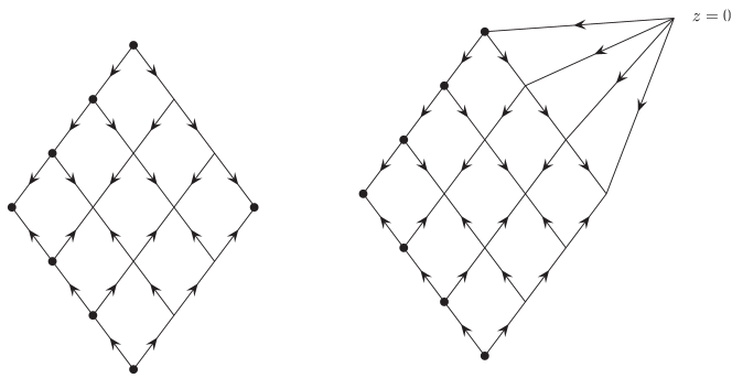
Figure 2: Examples of diagrams for scalar products, equations (4.3), (4.11) for $N=4$.

Appendix C Gustafson’s integral reduction

The extension of the first Gustafson integral [26, Theorem 5.1] to the complex case was obtained in [16]. It takes the form

$$\prod_{j=1}^{N}\sum_{n_{j}\in\mathbb{Z}+\frac{\sigma}{2}}\int_{-{\rm i}\infty}^{{\rm i}\infty}\frac{\prod_{m=1}^{N+1}\prod_{k=1}^{N}\boldsymbol{\Gamma}(z_{m}-u_{k})\boldsymbol{\Gamma}(u_{k}+w_{m})}{\prod_{m<j}\boldsymbol{\Gamma}(u_{m}-u_{j})\boldsymbol{\Gamma}(u_{j}-u_{m})}\prod_{p=1}^{N}\frac{{\rm d}\nu_{p}}{2\pi{\rm i}}$$

$$\qquad=\frac{N!\prod_{k,j=1}^{N+1}\boldsymbol{\Gamma}(z_{k}+w_{j})}{\boldsymbol{\Gamma}\left(\sum_{k=1}^{N+1}(z_{k}+w_{k})\right)},$$ (C.1)

where $\boldsymbol{\Gamma}$ is the Gamma function of the complex field $\mathbb{C}$ [20]

$$\boldsymbol{\Gamma}(u)\equiv\boldsymbol{\Gamma}(u,\bar{u})=\frac{\Gamma(u)}{\Gamma(1-\bar{u})}=\frac{1}{a(u)}.$$

The variables $u_{k}$, $w_{m}$, $z_{m}$ have the form

$$u_{k}=\frac{n_{k}}{2}+\nu_{k},\qquad z_{m}=\frac{n_{m}}{2}+x_{m},\qquad w_{m}=\frac{\ell_{m}}{2}+y_{m},$$

$$\bar{u}_{k}=-\frac{n_{k}}{2}+\nu_{k},\qquad \bar{z}_{m}=-\frac{n_{m}}{2}+x_{m},\qquad \bar{w}_{m}=-\frac{\ell_{m}}{2}+y_{m}.$$

and the integration contours over $\nu_{k}$ separate the series of poles associated with the $\boldsymbol{\Gamma}$-functions: $\boldsymbol{\Gamma}(z_{m}-u_{k})$ and $\boldsymbol{\Gamma}(u_{k}+w_{m})$, see [16] for more detail. The integral converges for

$$\sum_{m=1}^{N+1}\mathrm{Re}(z_{m}+w_{m})<1.$$

Let us put

$$z_{N+1}=M\left(\frac{1}{2}+{\rm i}x\right),\qquad \bar{z}_{N+1}=M\left(-\frac{1}{2}+{\rm i}x\right),$$

$$w_{N+1}=M^{\prime}\left(\frac{1}{2}+{\rm i}x^{\prime}\right),\qquad \bar{w}_{N+1}=M^{\prime}\left(-\frac{1}{2}+{\rm i}x^{\prime}\right)$$

and send $M,M^{\prime}\to\infty$ keeping $M/M^{\prime}=\xi$ fixed, so that $w_{N+1}/z_{N+1}\mapsto\zeta$ and $\bar{w}_{N+1}/\bar{z}_{N+1}\mapsto\bar{\zeta}$.

Dividing both sides of (C.1) by $(\boldsymbol{\Gamma}(z_{N+1})\boldsymbol{\Gamma}(w_{N+1}))^{N}$, we get in this limit

$$\frac{1}{N!}\prod_{j=1}^{N}\sum_{n_{j}\in\mathbb{Z}+\frac{\sigma}{2}}\int_{-{\rm i}\infty}^{{\rm i}\infty}[\zeta]^{U}\frac{\prod_{m,k=1}^{N}\boldsymbol{\Gamma}(z_{m}-u_{k})\boldsymbol{\Gamma}(u_{k}+w_{m})}{\prod_{m<j}\boldsymbol{\Gamma}(u_{m}-u_{j})\boldsymbol{\Gamma}(u_{j}-u_{m})}\prod_{p=1}^{N}\frac{{\rm d}\nu_{p}}{2\pi{\rm i}}$$

$$\qquad=\frac{[\zeta]^{Z}}{[1+\zeta]^{Z+W}}\prod_{k,j=1}^{N}\boldsymbol{\Gamma}(z_{k}+w_{j}),$$ (C.2)

where $|\arg\zeta|<\pi$, $Z=\sum_{k=1}^{N}z_{k}$, $W=\sum_{k=1}^{N}w_{k}$ and we recall that $[\zeta]^{U}\equiv\zeta^{U}\bar{\zeta}^{\bar{U}}$.

Acknowledgements

The author is grateful to S.É. Derkachov for fruitful discussions and T.A. Sinkevich for critical remarks.

References

- [1] Bartels J., Lipatov L.N., Prygarin A., Integrable spin chains and scattering amplitudes, J. Phys. A 44 (2011), 454013, 29 pages, arXiv:1104.0816.
- [2] Bytsko A.G., Teschner J., Quantization of models with non-compact quantum group symmetry: modular magnet and lattice sinh-Gordon model, J. Phys. A 39 (2006), 12927–12981, arXiv:hep-th/0602093.
- [3] Cavaglià A., Gromov N., Levkovich-Maslyuk F., Separation of variables and scalar products at any rank, J. High Energy Phys. 2019 (2019), no. 9, 052, 28 pages, arXiv:1907.03788.
- [4] Derkachov S., Kazakov V., Olivucci E., Basso–Dixon correlators in two-dimensional fishnet CFT, J. High Energy Phys. 2019 (2019), no. 4, 032, 31 pages, arXiv:1811.10623.
- [5] Derkachov S., Olivucci E., Exactly solvable magnet of conformal spins in four dimensions, Phys. Rev. Lett. 125 (2020), 031603, 7 pages, arXiv:1912.07588.
- [6] Derkachov S., Olivucci E., Conformal quantum mechanics & the integrable spinning Fishnet, J. High Energy Phys. 2021 (2021), no. 11, 060, 29 pages, arXiv:2103.01940.
- [7] Derkachov S., Olivucci E., Exactly solvable single-trace four point correlators in , J. High Energy Phys. 2021 (2021), no. 2, 146, 86 pages, arXiv:2007.15049.
- [8] Derkachov S.E., Baxter’s -operator for the homogeneous spin chain, J. Phys. A 32 (1999), 5299–5316, arXiv:solv-int/9902015.
- [9] Derkachov S.E., Korchemsky G.P., Manashov A.N., Noncompact Heisenberg spin magnets from high-energy QCD. I. Baxter -operator and separation of variables, Nuclear Phys. B 617 (2001), 375–440, arXiv:hep-th/0107193.
- [10] Derkachov S.E., Korchemsky G.P., Manashov A.N., Baxter -operator and separation of variables for the open spin chain, J. High Energy Phys. 2003 (2003), no. 10, 053, 31 pages, arXiv:hep-th/0309144.
- [11] Derkachov S.E., Korchemsky G.P., Manashov A.N., Separation of variables for the quantum spin chain, J. High Energy Phys. 2003 (2003), no. 7, 047, 30 pages, arXiv:hep-th/0210216.
- [12] Derkachov S.E., Kozlowski K.K., Manashov A.N., On the separation of variables for the modular magnet and the lattice sinh-Gordon models, Ann. Henri Poincaré 20 (2019), 2623–2670, arXiv:1806.04487.
- [13] Derkachov S.E., Kozlowski K.K., Manashov A.N., Completeness of SoV representation for spin chains, SIGMA 17 (2021), 063, 26 pages, arXiv:2102.13570.
- [14] Derkachov S.E., Manashov A.N., Iterative construction of eigenfunctions of the monodromy matrix for magnet, J. Phys. A 47 (2014), 305204, 25 pages, arXiv:1401.7477.
- [15] Derkachov S.E., Manashov A.N., Spin chains and Gustafson’s integrals, J. Phys. A 50 (2017), 294006, 20 pages, arXiv:1611.09593.
- [16] Derkachov S.E., Manashov A.N., On complex gamma-function integrals, SIGMA 16 (2020), 003, 20 pages, arXiv:1908.01530.
- [17] Derkachov S.E., Valinevich P.A., Separation of variables for the quantum spin magnet: eigenfunctions of Sklyanin -operator, J. Math. Sci. 242 (2019), 658–682, arXiv:1807.00302.
- [18] Faddeev L.D., How algebraic Bethe ansatz works for integrable model, in Symétries Quantiques (Les Houches, 1995), North-Holland, Amsterdam, 1998, 149–219, arXiv:hep-th/9605187.
- [19] Faddeev L.D., Korchemsky G.P., High energy QCD as a completely integrable model, Phys. Lett. B 342 (1195), 311–322, arXiv:hep-th/9404173.
- [20] Gel’fand I.M., Graev M.I., Retakh V.S., Hypergeometric functions over an arbitrary field, Russian Math. Surveys 59 (2004), 831–905.
- [21] Gel’fand I.M., Graev M.I., Vilenkin N.Y., Generalized functions. Vol. 5. Integral geometry and representation theory, Academic Press, New York, 1966.
- [22] Gromov N., Levkovich-Maslyuk F., Ryan P., Determinant form of correlators in high rank integrable spin chains via separation of variables, J. High Energy Phys. 2021 (2021), no. 5, 169, 79 pages, arXiv:2011.08229.
- [23] Gromov N., Levkovich-Maslyuk F., Sizov G., New construction of eigenstates and separation of variables for quantum spin chains, J. High Energy Phys. 2017 (2017), no. 9, 111, 39 pages, arXiv:1610.08032.
- [24] Gromov N., Primi N., Ryan P., Form-factors and complete basis of observables via separation of variables for higher rank spin chains, J. High Energy Phys. 2022 (2022), no. 11, 039, 53 pages, arXiv:2202.01591.
- [25] Gustafson R.A., Some -beta and Mellin–Barnes integrals with many parameters associated to the classical groups, SIAM J. Math. Anal. 23 (1992), 525–551.
- [26] Gustafson R.A., Some -beta and Mellin–Barnes integrals on compact Lie groups and Lie algebras, Trans. Amer. Math. Soc. 341 (1994), 69–119.
- [27] Gutzwiller M.C., The quantum mechanical Toda lattice. II, Ann. Physics 133 (1981), 304–331.
- [28] Izergin A.G., Korepin V.E., The quantum inverse scattering method approach to correlation functions, Comm. Math. Phys. 94 (1984), 67–92, arXiv:cond-mat/9301031.
- [29] Kharchev S., Lebedev D., Integral representation for the eigenfunctions of a quantum periodic Toda chain, Lett. Math. Phys. 50 (1999), 53–77, arXiv:hep-th/9910265.
- [30] Kharchev S., Lebedev D., Integral representations for the eigenfunctions of quantum open and periodic Toda chains from the QISM formalism, J. Phys. A 34 (2001), 2247–2258, arXiv:hep-th/0007040.
- [31] Kitanine N., Maillet J.M., Terras V., Correlation functions of the Heisenberg spin- chain in a magnetic field, Nuclear Phys. B 567 (2000), 554–582, arXiv:math-ph/9907019.
- [32] Korepin V.E., Calculation of norms of Bethe wave functions, Comm. Math. Phys. 86 (1982), 391–418.
- [33] Kozlowski K.K., Unitarity of the SoV transform for the Toda chain, Comm. Math. Phys. 334 (2015), 223–273, arXiv:1306.4967.
- [34] Kulish P.P., Sklyanin E.K., Quantum spectral transform method. Recent developments, in Integrable Quantum Field Theories (Tvärminne, 1981), Lecture Notes in Phys., Vol. 151, Springer, Berlin, 1982, 61–119.
- [35] Lipatov L.N., High-energy scattering in QCD and in quantum gravity and two-dimensional field theories, Nuclear Phys. B 365 (1991), 614–632.
- [36] Lipatov L.N., Asymptotic behavior of multicolor QCD at high energies in connection with exactly solvable spin models, JETP Lett. 59 (1994), 596–599, arXiv:hep-th/9311037.
- [37] Lipatov L.N., Integrability of scattering amplitudes in SUSY, J. Phys. A 42 (2009), 304020, 25 pages, arXiv:0902.1444.
- [38] Maillet J.M., Niccoli G., On quantum separation of variables, J. Math. Phys. 59 (2018), 091417, 47 pages, arXiv:1807.11572.
- [39] Maillet J.M., Niccoli G., Complete spectrum of quantum integrable lattice models associated to by separation of variables, J. Phys. A 52 (2019), 315203, 39 pages, arXiv:1811.08405.
- [40] Maillet J.M., Niccoli G., On quantum separation of variables beyond fundamental representations, SciPost Phys. 10 (2021), 026, 38 pages, arXiv:1903.06618.
- [41] Maillet J.M., Niccoli G., Vignoli L., On scalar products in higher rank quantum separation of variables, SciPost Phys. 9 (2020), 086, 64 pages, arXiv:2003.04281.
- [42] Ryan P., Integrable systems, separation of variables and the Yang–Baxter equation, Ph.D. Thesis, Trinity College Dublin, 2021, arXiv:2201.12057.
- [43] Ryan P., Volin D., Separated variables and wave functions for rational spin chains in the companion twist frame, J. Math. Phys. 60 (2019), 032701, 23 pages, arXiv:1810.10996.
- [44] Ryan P., Volin D., Separation of variables for rational spin chains in any compact representation, via fusion, embedding morphism and Bäcklund flow, Comm. Math. Phys. 383 (2021), 311–343, arXiv:2002.12341.
- [45] Sarkissian G.A., Elliptic and complex hypergeometric integrals in quantum field theory, Phys. Part. Nuclei Lett. 20 (2023), 281–286.
- [46] Semenov-Tian-Shansky M.A., Quantization of open Toda lattices, in Dynamical Systems VII, Encyclopaedia Math. Sci., Springer, Berlin, 1994, 226–259.
- [47] Silantyev A.V., Transition function for the Toda chain, Teoret. and Math. Phys. 150 (2007), 315–331, arXiv:nlin.SI/0603017.
- [48] Sklyanin E.K., The quantum Toda chain, in Nonlinear Equations in Classical and Quantum Field Theory (Meudon/Paris, 1983/1984), Lecture Notes in Phys., Vol. 226, Springer, Berlin, 1985, 196–233.
- [49] Sklyanin E.K., Quantum inverse scattering method. Selected topics, in Quantum Group and Quantum Integrable Systems, Nankai Lectures Math. Phys., World Scientific, River Edge, NJ, 1992, 63–97.
- [50] Sklyanin E.K., Tahtadzhan L.A., Faddeev L.D., Quantum inverse problem method. I, Teoret. and Math. Phys. 40 (1980), 688–706.
- [51] Slavnov N.A., Calculation of scalar products of wave functions and form-factors in the framework of the algebraic Bethe ansatz, Teoret. and Math. Phys. 79 (1989), 232–240.
- [52] Tahtadzhan L.A., Faddeev L.D., The quantum method for the inverse problem and the Heisenberg model, Russian Math. Surveys 34 (1979), no. 5, 11–68.
- [53] Valinevich P.A., Derkachev S.E., Kulish P.P., Uvarov E.M., Construction of eigenfunctions for a system of quantum minors of the monodromy matrix for an -invariant spin chain, Teoret. and Math. Phys. 189 (2016), 1529–1553.
- [54] Wallach N.R., Real reductive groups. II, Pure Appl. Math., Vol. 132, Academic Press, Inc., Boston, MA, 1992.