Team Coordination on Graphs with State-Dependent Edge Cost

Abstract

This paper studies a team coordination problem in a graph environment. Specifically, we incorporate “support” action which an agent can take to reduce the cost for its teammate to traverse some edges that have higher costs otherwise. Due to this added feature, the graph traversal is no longer a standard multi-agent path planning problem. To solve this new problem, we propose a novel formulation that poses it as a planning problem in the joint state space: the joint state graph (JSG). Since the edges of JSG implicitly incorporate the support actions taken by the agents, we are able to now optimize the joint actions by solving a standard single-agent path planning problem in JSG. One main drawback of this approach is the curse of dimensionality in both the number of agents and the size of the graph. To improve scalability in graph size, we further propose a hierarchical decomposition method to perform path planning in two levels. We provide complexity analysis as well as a statistical analysis to demonstrate the efficiency of our algorithm.

I INTRODUCTION

In this work, we are interested in designing coordinated group motion, where the safety or cost for one agent to move from one location to another may depend on the support provided by its teammate. As an example, let’s say there are two robots traversing an environment represented as a graph in Fig. 1. Starting from 1, the robots face a wall, represented by a red edge. The robots could either climb a ladder together and potentially fall and break (move from 1 to 4 together), or one robot could hold the ladder (support from 2) while the other moves up from 1 to 4. The former option is high risk, while the latter is low risk and preferable. Alternatively, if the ladder is bolted to the ground, then climbing together can be low risk and preferable. This paper develops a framework to study when such coordination is beneficial.

The terms cooperation and coordination take various meanings in different contexts. There is research done on the coordination of actions of agents to reach a state of order, such as consensus and formation control [1, 2, 3, 4, 5]. Others study cooperation in terms of simultaneously performing tasks in a spatially extended manner, like in surveillance [1, 6] and sampling [7]. Cooperation is also explored in problems where agents need to react locally to avoid conflict or collision, as can be seen in transportation systems on the road [8], in the air [9], and in general robotic cooperation problems [10, 11, 12]. We see in these situations that there is little coupling between the agents – agents do not rely on each other to make progress, but simply need to not be in each other’s paths. In this work, we are interested in tightly coupled agents that depend on each other for support in order to meet their objective.

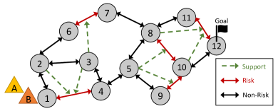
Figure 1: Example of an environment graph with risk edges and supporting nodes.

We study support in the context of mitigating some risks that exist in the environment. Such risk has been formulated and studied in various ways. For instance, probability of achieving certain levels of performance in a stochastic setting has been considered [13, 14, 15, 16]. Others have considered types of risk measures such as coherent risk measures [17], like conditional value-at-risk (CVaR) [18],[19] and entropic value-at-risk (EVAR) [20]. Risk can also be characterized in terms of chance constraints [21]. Game theory is considered to account for the risk associated with the uncertainty in the adversary’s behavior [22]. Yet, risk can purely be described as the “cost” of traversal [13]. In this work, we will only use this cost of traversal approach to simplify the analysis.

Cooperation has been studied both in centralized and distributed settings. Decentralized systems are better at handling scalability and computational efficieny [23, 24]. When it comes to Distributed Continual Planning (DCP) [25], plan generation and execution can happen concurrently. As it relies on communication between agents, it is better suited for online planning. On the other hand, centralized systems are better for offline planning [26]. It is less likely to suffer from communication costs, information loss, and synchronization issues [27]. A centralized approach is better suited for tightly coupled agents that require a high degree of coordination [28]. For that reason, we use a centralized approach in our work.

Since we take a centralized approach, ensuring computational tractability becomes a challenge. Approaches to simplifying a multi-agent planning problem have been widely studied, such as decomposition, graph reformulation, and others [29, 30, 28]. In our work, we develop a hierarchical decomposition method on a reformulated graph to solve a multi-agent path planning problem with high coordination.

The contribution of the paper are: (i) the formulation of a new multi-agent coordination problem with strong coupling between teammembers’ positions and action; (ii) a conversion of the problem into a simple single-agent path-planning problem; and (iii) development of a hierarchical decomposition scheme that alleviates the curse of dimensionality.

II PROBLEM FORMULATION

We consider a scenario where a team of robots must move from their initial locations to some goal locations. More specifically, we are interested in a situation where the cost of traversal is affected by the presence and actions of other team members. In the following, we will introduce the base graph, and then formulate how the edge cost changes based on the “support” provided by the teammate. For conciseness, we will restrict the discussion to a two-agent team, but the idea will generalize to a larger team size.

The environment is modeled as a graph where nodes represent key locations and the edges represent the traversability between them. The base graph is denoted by $\mathbb{G}=(\mathcal{V},\mathcal{E})$, where $\mathcal{V}$ is a set of nodes, and $\mathcal{E}$ is a set of edges, $\mathcal{E}\subset\mathcal{V}\times\mathcal{V}$. We assume $\mathbb{G}$ is strongly connected. The starting positions of the agents are denoted by the node set $\mathcal{V}_{0}\subset\mathcal{V}$. The robots seek to reach a set of goal nodes $\mathcal{V}_{g}\subset\mathcal{V}$ while minimizing the cost of traversal. The nominal cost for traversing the edge $e_{i,j}\in\mathcal{E}$ is a given constant, $c_{i,j}$ for $i,j\in\mathcal{V}$.

Let $I_{ab}$ denote a path (set of edges) from $a\in\mathcal{V}$ to $b\in\mathcal{V}$. We use $\psi_{a,b}$ to denote the minimum cost to move from $a$ to $b$:

$$\psi_{a,b}=\min_{I_{ab}}\sum_{e_{i,j}\in I_{ab}}c_{i,j}.$$ (1)

A standard path planning will simply consider this shortest path for each agent.

We now define the environment graph, which incorporates the notion of risk and support. Each edge $e_{i,j}$ is associated with a set of support nodes, $\mathcal{Z}_{i,j}\subseteq\mathcal{V}$. If this set is non-empty, then an agent at $v\in\mathcal{Z}_{i,j}$ can provide support for the agent traversing $e_{i,j}$. The action set for an agent $n\in\{A,B\}$ at node $i$ is given as $\mathcal{A}^{n}_{i}=\{\{a_{i,j}\}_{j\in\mathcal{N}_{i}},a_{s}\}$. Where $\mathcal{N}_{i}$ is the neighborhood of $i$, and $a_{i,j}$ is the action to move to node $j$ given that it is in the neighborhood of $i$. The action $a_{s}$ is the support. Note, if we were to consider a team size larger than two, we would have to explicitly denote which agent is being supported by $n$.

Let $p^{t}=(p^{t}_{A},p^{t}_{B})$ be the position of agents A and B at time $t$, and let $a^{t}=(a^{t}_{A},a^{t}_{B})$ be the actions agents A and B take at time $t$. The cost of an action for agent A is given as

$$c^{t}_{A}(\cdot)=\begin{cases}c_{i,j},&\text{if }a_{A}=a_{i,j}\text{ and }p_{B}\notin\mathcal{Z}_{i,j}\text{ or }a_{B}\neq a_{s},\\ \tilde{c}_{i,j},&\text{if }a_{A}=a_{i,j}\text{, }p_{B}\in\mathcal{Z}_{i,j}\text{, and }a_{B}=a_{s},\\ \tilde{c},&\text{if }a_{A}=a_{s},\\ 0,&\text{if }a_{A}\neq a_{s}\text{ and }a_{A}\neq a_{i,j},\end{cases}$$ (2)

where $(\cdot)$ represents the arguments $(p^{t},a^{t},\mathcal{Z}_{i,j})$.

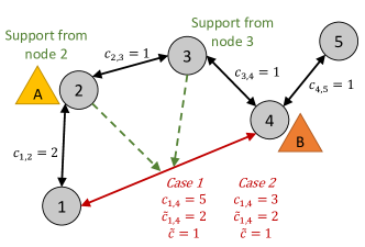
Figure 2: Illustrative example of an environment graph with a risk edge and supporting nodes. Case 1 has a high risk cost. Case 2 has a low risk cost.

For example, in Fig. 2, if at $t=1$ agent A is at node 2 (a supporting node) and provides support to agent B as the latter moves from node 1 to node 4, then the cost for agent A would be $c^{1}_{A}=\tilde{c}$ and the cost for agent B would be $c^{1}_{B}=\tilde{c}_{1,4}$. If both agents A and B move together from node 1 to node 4, the cost for the agents would be $c^{1}_{A}=c^{1}_{B}=c_{1,4}$.

In order to find the total cost at time $t$, we can simply sum the costs for both agents

$$C^{t}=c^{t}_{A}+c^{t}_{B}.$$ (3)

Let $\mathcal{R}^{n}=\{r^{n}_{1},...,r^{n}_{m}\}$ be the set of action sequences agent $n$ can take from start node to goal node. Where each sequence is the ordered set of actions taken from start to goal from $t=1$ to the time it takes for the agents to reach the goal state, $T$, i.e., $r^{n}_{m}=[a^{1}_{n},...a^{T}_{n}]$.

The sum of the costs for a given sequence of actions $r^{A}\in\mathcal{R}^{A}$, $r^{B}\in\mathcal{R}^{B}$ are

$$F(r^{A},r^{B})=\sum_{t=1}^{T}C^{t}.$$ (4)

The goal is to find a pair ($r^{A*},r^{B*}$) that minimizes the total cost, $F$:

$$\min_{r^{A}\in\mathcal{R}^{A},r^{B}\in\mathcal{R}^{B}}F.$$ (5)

An illustrative example in Fig. 2, where agents A and B need to reach goal node 5. To traverse the risk edge, they either use or do not use support depending on how costly, or risky, the edge is. Agents demonstrate supporting behavior in Case 1. If agent B traverses risk edge $e_{1,4}$ without support from A, the cost for B would be $c_{1,4}=5$. With support from A, the reduced cost for B would be $\tilde{c}_{1,4}=2$. The total cost at this time step $t$ is $C^{t}=\tilde{c}_{1,4}+\tilde{c}=2+1=3$. Thus, agents in this case accrue less costs by supporting each other. Case 2 is a scenario where the agents do not show supporting behavior in a low risk situation. Since $c_{1,4}=3$, B can traverse $e_{1,4}$ without support from A. The total cost at this time step $t$ is $C^{t}=c_{1,4}+0=3+0=3$ without A’s support.

One way to solve the minimization problem in (5) is by posing it as an instance of MDP. However, we will introduce a simplification using the concept of Joint State Graph in the next section.

III METHOD

We first introduce the concept of Joint State Graph (JSG) which simplifies the joint action selection problem into a standard path planning problem on graphs. To improve scalability, we propose in III-B a method of decomposing JSG to deal with scalability of the graph. Finally, we conclude the section with a complexity analysis.

III-A Joint State Graph

The problem described in the previous section can be solved using MDP. However, we propose transforming the environment graph into a joint state space graph. The paths on the JSG inherit the actions of the agents, which means we no longer need to consider the action sets. This makes the problem simpler than MDP. Let the JSG be a graph $\mathbb{J}=(\mathcal{S},\mathcal{L})$, where $\mathcal{S}=\{s_{ij}:i,j\in\mathcal{V}\}$ is the set of nodes representing joint states, and $\mathcal{L}$ is the set of edges.

Let $s_{11}$ be the initial state assuming that $\mathcal{V}_{0}=(1,1)$. Let $s_{gg}$ be the goal state. Edges on JSG are denoted as $e_{ij,wk}=(s_{ij},s_{wk})$ if agent A can move from $i$ to $w$ in the base graph, and agent B can move from $j$ to $k$, i.e., $e_{i,w}\in\mathcal{E}$ and $e_{j,k}\in\mathcal{E}$. If agent A does not move, we have $i=w$. Similarly, if B does not move, $j=k$.

Let $\mathcal{C}$ be the set of costs for each edge on the JSG, where an element is denoted as $C_{ij,wk}$. If A remains at $i\in\mathcal{Z}_{j,k}$ while B traverses from $j$ to $k\in\mathcal{N}_{j}$, the cost is defined as $C_{ij,ik}=\min\{c_{j,k},(\tilde{c}_{j,k}+\tilde{c})\}$. This is how the edge in JSG subsumes the action selection in the original problem. However, if $i\notin\mathcal{Z}_{j,k}$, then the cost is simply $C_{ij,ik}=c_{j,k}$. The case when A moves is defined similarly. This explains lines 7-17 of Algorithm 1. If A traverses from $i$ to $w\in\mathcal{N}_{i}$ and B traverses from $j$ to $k\in\mathcal{N}_{j}$, then we add the nominal costs $C_{ij,wk}=c_{i,w}+c_{j,k}$. In the case that both agents are stationary, the cost is $C_{ij,ij}=0$ The details of the JSG construction are in Algorithm 1.

Let $\mathcal{U}=\{u_{1},...,u_{m}\}$ be the set of paths on the JSG, where an element $u=\{e_{11,kw},...,e_{ij,gg}\}$ is the set of edges from the initial state to the goal state. Then, the cost of each path $u$ is given by the sum of the cost of the edges on that path in JSG,

$$Q({u})=\sum_{e_{ij,wk}\in u}C_{ij,wk}.$$ (6)

Using a standard shortest-path algorithm, we can find the optimal path that minimizes $Q({u})$:

$$Q({u}^{\star})=\min_{u\in\mathcal{U}{}}Q({u}).$$ (7)

An example of JSG is shown in Fig. 3,

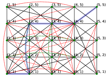
Figure 3: Code-generated Joint State Graph from the 5-node environment graph. Black edges are non-risky edges, red edges are risk with no support, and green edges are risk with support.

which corresponds to the environment graph shown in Fig. 2. The edges highlighted in blue indicates the optimal path $u^{\star}$ for Case 1 in Fig. 2. Importantly, we can easily identify the original actions from the edges selected in this JSG: e.g., the use of edge $e_{21,24}$ indicates that A at node 2 supported B who moved from node 1 to 4.

Although planning on JSG is conceptually simple, it can become computationally expensive with greater graph sizes. The next section addresses this issue.

1 Input $\mathbb{G}=(\mathcal{V},\mathcal{E})$, $\mathcal{Z}_{i,j}$.

2 Let $\mathbb{J}=(\mathcal{S},\mathcal{L})$

3 for $\forall i,j\in\mathcal{V}$ do

4       Add $s_{ij}$ to $\mathcal{S}$

5 end for

6for any two distinct elements $s_{ij},s_{wk}\in\mathcal{S}$ do

7      if $i=w$, $j\neq k$ and $k\in\mathcal{N}_{j}$  then

8            if $i\in$ $\mathcal{Z}_{jk}$  then

9                   Add edge $e_{ij,wk}$ to $\mathcal{L}$. Define its cost as $C_{ij,wk}=\min\{c_{j,k},(\tilde{c}_{j,k}+\tilde{c})\}$

10                  

11             else

12                   Add edge $e_{ij,wk}$ to $\mathcal{L}$. Define its cost as $C_{ij,wk}=c_{j,k}$

13                  

14             end if

15            

16       else if $i\neq w$, $j=k$ and $w\in\mathcal{N}_{i}$ then

17            if $j\in\mathcal{Z}_{iw}$ then

18                   Add edge $e_{ij,wk}$ to $\mathcal{L}$. Define its cost as $C_{ij,wk}=\min\{c_{i,w},(\tilde{c}_{i,w}+\tilde{c})\}$

19                  

20             else

21                   Add edge $e_{ij,wk}$ to $\mathcal{L}$. Define its cost as $C_{ij,wk}=c_{i,w}$

22                  

23             end if

24            

25       else if $k\in\mathcal{N}_{j}$ and $w\in\mathcal{N}_{i}$ then

26             Add edge $e_{ij,wk}$ to $\mathcal{L}$. Define its cost as $C_{ij,wk}=c_{i,w}+c_{j,k}$

27       end if

28      

29 end for

Return $\mathbb{J}=(\mathcal{S},\mathcal{L})$ and the associated costs $C_{ij,wk}$.

Algorithm 1 JSG Construction.

III-B Search Algorithm: Critical Joint State graph

In this section, we introduce a new search algorithm based on constructing a Critical Joint State Graph (CJSG), which has reduced computational complexity compared with the straightforward JSG method in Sec. III-A. Note that the Joint State Graph $\mathbb{J}$ has $|S|=|\mathcal{V}|^{2}$ number of nodes, leading to high complexity if directly used for planning. To address this issue, our key idea is to classify the agents’ movements into coupled and decoupled modes, where only the coupled movements need to be planned on a joint state representation, and the decoupled movements can be independently planned by each agent on base graph $\mathbb{G}$. As visualized in Fig. 4, the environment graph formulated in Sec. II builds on a base graph $\mathbb{G}$, then associates some of its edges with a set ($\mathcal{Z}_{i,j}$) of support nodes. Depending on whether the edges in $\mathbb{G}$ have at least one support node, we define a risk edge set $\mathcal{E}_{R}$ such that $\forall e_{i,j}\in\mathcal{E}_{R}$, $\mathcal{Z}_{i,j}\neq\emptyset$. Note that the support graph in Fig. 4 does not follow the standard ‘graph’ definition in mathematics. It only describes a supporting relationship between nodes and risk edges which we use later to study coupled movements of agents.

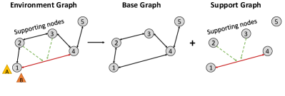
Figure 4: Example for environment graph decomposition. In $\mathbb{G}$, node 2 and node 3 can support the edge between node 1 and node 4.

We start by considering the costs for decoupled movements of the two agents. Recall that $\psi_{a,b}$ denotes the minimum cost for an agent to move from $a$ to $b$ on the base graph $\mathbb{G}$, the following statement holds.

Lemma 1.

(Decoupled planning on base graph): On graph $\mathbb{G}$, consider the first agent moves from node $i$ to $w$; the second agent moves from node $j$ to $k$. Let $R_{ij,wk}$ be the minimum cost for the two agents to complete the movement without performing supporting behaviors. Then

$$R_{ij,wk}=\psi_{i,w}+\psi_{j,k}.$$

Proof.

The proof is trivial. Since the two agents do not perform supporting behaviors, their movements and associated costs can be computed individually on the base graph $\mathbb{G}$, which by definition are $\psi_{i,w}$ and $\psi_{j,k}$. ∎

Now, to characterize the coupled movements of the two agents, we construct a Critical Joint State Graph (CJSG), $\mathbb{T}=(\mathcal{M},\mathcal{H})$, where $\mathcal{M}$ and $\mathcal{H}$ are the node set and edge set of $\mathbb{T}$, respectively. For any $h_{ij,wk}\in\mathcal{H}$, let $W_{ij,wk}$ denote the cost associated with this edge. Details of CJSG construction are summarized in Algorithm 2.

1 Input $\mathcal{E}_{R}$, $s_{11}$, $s_{gg}$, $\mathcal{Z}_{i,j},R_{ij,wk}$.

2 Let $\mathbb{T}=(\mathcal{M},\mathcal{H})$

3 for each $e_{i,j}\in\mathcal{E}_{R}$ do

4      for each $k\in\mathcal{Z}_{i,j}$ do

5             Add $s_{ki}$ and $s_{kj}$ to $\mathcal{M}$.

6             Add $s_{ik}$ and $s_{jk}$ to $\mathcal{M}$.

7            

8       end for

9      Add $s_{11}=(1,1)$ and $s_{gg}=(g,g)$ to $\mathcal{M}$ (if they are not already in $\mathcal{M}$).

10       for any two distinct elements $s_{ij},s_{wk}\in\mathcal{M}$ do

11            if  $e_{j,k}\in\mathcal{E}_{R}$ and $i=w\in\mathcal{Z}_{j,k}$  then

12                  Add edge $h_{ij,wk}$ to $\mathcal{H}$. Define its cost as $W_{ij,wk}=\min\{(\tilde{c}_{j,k}+\tilde{c}),R_{ij,wk}\}$

13                  

14             else if $e_{i,w}\in\mathcal{E}_{R}$ and $j=k\in\mathcal{Z}_{i,w}$ then

15                  Add edge $h_{ij,wk}$ to $\mathcal{H}$. Define its cost as $W_{ij,wk}=\min\{(\tilde{c}_{i,w}+\tilde{c}),R_{ij,wk}\}$.

16             else

17                   Add edge $h_{ij,wk}$ to $\mathcal{H}$. Define the associated cost as $W_{ij,wk}=R_{ij,wk}$.

18             end if

19            

20       end for

21      

22 end for

Return $\mathbb{T}=(\mathcal{M},\mathcal{H})$ and the associated costs $W_{ij,wk}$.

Algorithm 2 CJSG Construction

Remark 1.

(Algorithm 2 explained): In CJSG, we consider the node of the graph as any joint state that the two agents (i) can initiate or complete supporting behaviors (c.f. steps 2 and 2), (ii) at their start or goal position of the planning task (c.f. step 2). We let CJSG be fully connected. The edge costs are associated with two agents moving over the base graph (c.f. step 2) or a possible lower cost when they perform a support behavior (c.f. steps 2 or 2, depending on who supports who).

To provide a toy example, given the environment graph in Fig. 4, we can construct the corresponding CJSG as shown in Fig. 5. Using the support graph, the critical joint states are the highlighted states in the middle part of Fig. 5 as well as the initial and goal states. By computing edge costs according to Lemma 1 and Algorithm 2, the CJSG is constructed as shown on the right side of Fig. 5. Red edges are edges under supporting behaviors such that $\tilde{c}_{j,k}$ and $\tilde{c}_{i,w}$ are available. The blue edges are associated with $R_{ij,wk}$ where two agents are decoupled and individually seek optimal paths on the base graph.

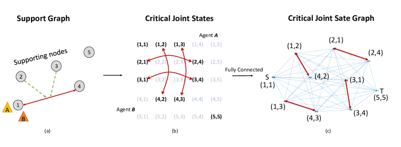
Figure 5: Example for CJSG Construction. Based on support graph in (a), we can observe all critical joint states as depicted in (b). By fully connecting these critical joint states with the initial states and goal states, we obtain the CJSG $\mathbb{T}$ as shown in (c).

After constructing CJSG, we present our search algorithm. We define a path composition operation. Suppose $u_{1}=\{e_{a,b},e_{c,d},\cdots,e_{i,j}\}$, $u_{2}=\{e_{g,h},e_{r,t},\cdots,e_{k,\ell}\}$. Then $u_{1}\oplus u_{2}=\{e_{ag,bh},e_{cr,dt},\cdots,e_{il,j\ell}\}$. When the two paths do not have the same length, we extend the shorter one by repeating its final node (so that in the graph representation, it stays at that node). For example, if $u_{1}$ is two elements shorter than $u_{2}$ then we extend it by $u_{1}=\{e_{a,b},e_{c,d},\cdots,e_{i,j},e_{j,j},e_{j,j}\}$. The length of the composed path equals the length of the $u_{1}$ or $u_{2}$, whichever is longer. Based on CJSG and path composition, our search algorithm is presented in Algorithm 3, where PathPL can be any path planning algorithm, i.e., Dijkstra’s algorithm [31], that can obtain a shortest path between two nodes.

1 Input $\mathbb{T}=(\mathcal{M},\mathcal{H})$, $\mathbb{G}=(\mathcal{V},\mathcal{E})$.

2 $\widehat{u}\leftarrow$ PathPL($\mathbb{T}$, $s_{11}$, $s_{gg}$)

3 for each ${h}_{ij,wk}$ in $\widehat{u}$ do

4       if  $W_{ij,wk}=R_{ij,wk}$  then

5            Add [PathPL$(\mathbb{G},i,w)$$\oplus$PathPL$(\mathbb{G},i,k)$)] to ${u}^{\dagger}$

6       else if  $W_{ij,wk}=\tilde{c}_{i,w}+\tilde{c}$ or $W_{ij,wk}=\tilde{c}_{j,k}+\tilde{c}$  then

7            Add $[e_{ij,wk}]$ to ${u}^{\dagger}$

8       end if

9      

10 end for

Return ${u}^{\dagger}$.

Algorithm 3 Path Planning based on CJSG.

Remark 2.

(Algorithm 3 explained): We first perform path planning on $\mathbb{T}$. Note that some edges ${h}_{ij,wk}$, when $W_{ij,wk}=R_{ij,wk}$, are associated with paths of two agents planned in $\mathbb{G}$ using Lemma 1. We use step 3 to reconstruct these edges back to paths that the agents can traverse on the environment. Furthermore, although step 3 recalls a path planning process, this planning should have already been computed by Lemma 1 when executing Algorithm 2.

Lemma 2.

(Effectiveness of the critical-joint state graph): The following statements hold.
(i) Any path ${u}^{\dagger}$ reconstructed from a path $\widehat{u}$ on CJSG is a feasible path for the two agents on the environment graph, thus, $Q({u}^{\dagger})\geq Q({u}^{\star})$.
(ii) The optimal path planned from the CJSG has the same minimum cost as the optimal path planned directly from the JSG, thus, $Q({u}^{\dagger})\leq Q({u}^{\star})$.

Proof.

We prove the two statements in Lemma 2.
(i) Given any edge $e_{ij,wk}$ in path ${u}^{\dagger}$, there are two situations. One is $W_{ij,wk}=\tilde{c}_{i,w}+\tilde{c}$ or $W_{ij,wk}=\tilde{c}_{j,k}+\tilde{c}$, and another is $W_{ij,wk}=R_{ij,wk}$. For the first case, the path in the environment graph represents one agent staying at the support node where another agent traverses the corresponding supported edge. It is a feasible path for two agents on the environment graph by definition. For the second case, according to Lemma 1, two agents move independently and decoupled. As each agent moves from one node to another on the environment graph, the path obtained from the algorithm is feasible since the planned base graph $\mathbb{G}$ is a subgraph of the environment graph. Therefore, $u^{\dagger}$ is always a feasible path for two agents on the environment graph. Since $u^{\star}$ is the optimal path for the environment graph planned from the JSG, we have $Q({u}^{\dagger})\geq Q({u}^{\star})$.
(ii) We prove this by showing that for any optimal path planned from the JSG, there is a path on CJSG with the same cost. Considering the optimal path planned from JSG, it consists of two agents’ movements with and (possibly) without supporting behaviors. Let the $u^{\star}$ be divided into different segments according to the above attribute. It is obvious that all such segments are connected by a joint state that initiates the supporting behavior and a state that completes the supporting behavior, which are essentially critical-joint states. Therefore, if we consider each segment independently, the optimal path over this segment must always be associated with the edges on the CJSG, either in the form of decoupled paths on the base graph or by performing a supporting behavior. Thus, for any optimal path planned from the JSG, there is a path on CJSG with the same cost. This together with the fact that ${u}^{\dagger}$ is the optimal path on CJSG leads to the conclusion $Q({u}^{\dagger})\leq Q({u}^{\star})$. We complete the proof. ∎

III-C Comparison of Computational Complexity

We quantify the computational complexity of the search algorithm applied to the joint state graph (JSG) and the critical joint state graph (CJSG), to demonstrate the advantage of CJSG over the JSG.

For JSG $\mathbb{J}=(\mathcal{S},\mathcal{L})$ the graph construction complexity is given by the addition of complexities of nodes and edges. The complexity for the nodes is $\mathcal{O}(|\mathcal{S}|)=\mathcal{O}(|\mathcal{V}|^{2})$. Similarly, the complexity of edges is $\mathcal{O}(|\mathcal{L}|)$ which equals $\mathcal{O}(|\mathcal{V}|^{4})$ in worst case senario when edges are fully connected. Thus, the graph construction complexity of JSG equals

$$\mathcal{O}_{\text{Jconst}}=\mathcal{O}(|\mathcal{V}|^{2})+\mathcal{O}(|\mathcal{V}|^{4}).$$ (8)

Since the total number of nodes in JSG is $\mathcal{O}(|\mathcal{V}|^{2})$, the search complexity when edges are fully connected follows

$$\mathcal{O}_{\text{Jplan}}=\mathcal{O}(|\mathcal{V}|^{4}).$$ (9)

Combining equations (8) and (9), complexity of JSG becomes

$$\mathcal{O}_{\text{JSG}}=\mathcal{O}(|\mathcal{V}|^{4}).$$ (10)

Similarly, the construction complexity of CJSG $\mathbb{T}=(\mathcal{M},\mathcal{H})$ can be expressed as the addition of construction complexities for nodes and edges. For nodes, the complexity simply equals $\mathcal{O}(|\mathcal{M}|)$. For edges, the complexity equals $\mathcal{O}(|\mathcal{M}|^{2})+\mathcal{O}(|\mathcal{V}|^{2}\log(|\mathcal{V}|))$, where the first term is the number of edges in $\mathbb{T}$, which is fully connected. The second term comes from Lemma 1, which, in the worst case, needs to compute the shortest path between any pair of nodes in $\mathbb{G}$. The complexity of $\mathcal{O}(|\mathcal{V}|^{2}\log(|\mathcal{V}|))$ assumes the use of Johnson’s algorithm [31]. Thus, the construction complexity of CJSG equals

$$\mathcal{O}_{\text{const}}=\mathcal{O}(|\mathcal{M}|)+\mathcal{O}(|\mathcal{M}|^{2})+\mathcal{O}(|\mathcal{V}|^{2}\log(|\mathcal{V}|)).$$ (11)

The search complexity of CJSG is determined by the number of nodes in $\mathbb{T}$, which follows

$$\mathcal{O}_{\text{plan}}=\mathcal{O}(|\mathcal{M}|^{2})+\mathcal{O}(|\mathcal{M}|).$$ (12)

where for the first term, we assume the use of Dijkstra’s Algorithm [31] on $\mathbb{T}$, to obtain $\widehat{u}$. The second term is associated with reconstructing $u^{\dagger}$ from $\widehat{u}$. Although Algorithm 3 embeds search functions in step 3, all the planning must have been computed by Lemma 1 when executing Algorithm 2. No replanning is needed. By combining (11) and (12), one has

$$\mathcal{O}_{\text{CJSG}}=\mathcal{O}(|\mathcal{M}|^{2})+\mathcal{O}(|\mathcal{V}|^{2}\log(|\mathcal{V}|)).$$ (13)

Remark 3.

(Comparison of complexity): To compare the complexities of $\mathcal{O}_{\text{CJSG}}$ and $\mathcal{O}_{\text{JSG}}$, we only need to compare $\mathcal{O}(|\mathcal{M}|^{2})$ and $\mathcal{O}(|\mathcal{V}|^{4})$. Note that in most scenarios, we assume the number of support edges in $\mathbb{G}$ is small. As a consequence, the number of critical-joint states is far less than that of common joint states, i.e. $|\mathcal{M}|\ll|\mathcal{V}|^{2}$. Then the proposed Algorithm 3 based on CJSG is significantly more efficient than the traditional JSG method. The worst boundary scenario happens when support edges widely exist in $\mathbb{G}$, in this case, one has $|\mathcal{M}|\to|\mathcal{V}|^{2}$, but $|\mathcal{M}|$ is still upper bounded by $|\mathcal{V}|^{2}$ due to the fact that critical joint states are subsets of joint states. Thus, $\mathcal{O}_{\text{CJSG}}$ is always no worse than $\mathcal{O}_{\text{JSG}}$.

IV NUMERICAL RESULTS

In this section, we evaluate JSG and CJSG on the basis of graph construction and path planning under different conditions. Our experimental design allows us to gain insights through comparative analysis of JSG and CJSG in terms of scalability and performance. The experiments are carried out on a MacBook Pro with 2.8 GHz 8 core CPU and 8GB of RAM.

For both graph construction and path planning analyses, a random graph generator is used to generate environment graphs with varying number of nodes and edges. We control the ratio of risk edges to the total edges to be 1/5, 1/3, and 1/2. For different number of nodes and risk edges ratio in an environment graph, we calculate graph construction time and shortest path planning time for JSG and CJSG (Table I). We repeat every experiment trial five times for statistical significance.

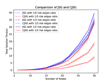
Figure 6: Comparison of time taken by JSG and CJSG to generate total solution with respect to increasing number of nodes and risk edges ratio.

TABLE I: Comparison of JSG and CJSG

		JSG		CJSG
Nodes	Risk Edges Ratio	Graph Construction(s)	Shortest Path(s)	Graph Construction(s)	Shortest Path(s)
10	1/5	0.2119$\pm$0.0410	0.1440$\pm$0.0176	0.0146$\pm$0.0021	0.0198$\pm$0.0152
	1/3	0.1760$\pm$0.0519	0.1510$\pm$0.0040	0.0895$\pm$0.0151	0.1258$\pm$0.0207
	1/2	0.1906$\pm$0.0273	0.1567$\pm$0.0091	0.1810$\pm$0.0143	0.1469$\pm$0.0478
20	1/5	3.1662$\pm$0.0405	2.098$\pm$0.0445	0.6525$\pm$0.0931	0.4348$\pm$0.0651
	1/3	3.3989$\pm$0.0603	2.1988$\pm$0.0660	1.7742$\pm$0.0497	0.7988$\pm$0.0094
	1/2	3.8566$\pm$0.0906	2.3192$\pm$0.0265	3.6439$\pm$0.5942	1.2523$\pm$0.1181
30	1/5	20.9363$\pm$0.8312	11.6431$\pm$0.12776	6.1126$\pm$0.5537	2.7973$\pm$0.1778
	1/3	22.4891$\pm$1.7074	12.3330$\pm$0.4995	13.8171$\pm$0.7259	4.5996$\pm$0.2204
	1/2	25.9774$\pm$0.4323	13.4440$\pm$0.14222	26.8156$\pm$1.49423	6.9094$\pm$0.2677

IV-A Graph Construction Analysis

From Table I, we analyze the graph construction time for JSG and CJSG under different conditions. Given a fixed risk edges ratio, e.g., 1/3 of the total edges, the improvement in graph construction time by CJSG compared to JSG maintains as the number of nodes increases from 10 to 30. Similarly, if we fix the number of nodes, e.g., 10, and increase the risk edges ratio gradually from 1/5, then 1/3, and finally 1/2, CJSG still takes less time compared to JSG. We can also see such a pattern for node 20 and node 30. These results provide empirical evidence that CJSG is more efficient in constructing graphs. Note that when the risk edge ratio reaches 1/2, nearly all joint states are critical joint states, i.e., $|\mathcal{M}|\to|\mathcal{V}|^{2}$, and the graph construction times for the two approaches are close to each other. This observation is in line with Remark 3.

IV-B Path Planning Analysis

From Table I, we also assess the path planning time for JSG and CJSG with varying nodes and risk edges ratio. Given a certain risk edges ratio, e.g., 1/3, we can see that CJSG takes less time than JSG. This is true even if we increase the nodes from 10 to 30. Similarly, if we fix the node size, e.g., 20, and gradually increase the risk edges ratio as 1/5, 1/3, and 1/2 of total edges, CJSG is still more efficient than JSG. We can see the same pattern for nodes 10, 20 and 30. These results indicate that CJSG is more efficient than JSG in terms of shortest path planning when the ratio of risk edges to nodes increases.

Based on the experimental results shown in Table I, we compute the total time taken by both JSG and CJSG to find the final solution. The total time involves time taken for graph construction and shortest path planning. In Fig. 6, we show that as the number of nodes increases, the time to generate total solution for JSG increases more significantly than that of CJSG. Fig. 6 also illustrates that as the risk edges ratio increases, the time to generate solution for JSG increases more significantly compared to CJSG. Thus, CJSG is more efficient than JSG for overall solution generation.

V CONCLUSIONS

We presented a team coordination problem in a graph environment, where high levels of coordination in the form of “support” allows agents to reduce the cost of traversal on some edges. As an alternative to solving this with a version of MDP, we presented a method of planning in the joint state space – the Joint State Graph (JSG). We showed that a multi-agent path planning problem can be reduced to a single-agent planning in JSG, since the actions taken by the agents are built in to the edges of the JSG. We addressed the issue of scalability in the graph size by presenting a hierarchical decomposition method to perform path planning in two levels. We provided complexity and statistical analysis which show that the construction time for both CJSG and JSG do not differ by much, but the CJSG is significantly more efficient with regards to shortest path planning. Our numerical results verify this.

For future work, there are many aspects of the problem we proposed that we are intrigued to build upon. For instance, we would like to integrate more sophisticated notions of risk by using concepts from game theory and incorporating stochasticity in the formulation, such as stochastic costs. We are also interested in addressing the issue of scalability in terms of number of agents.

References

- [1] P. R. Chandler, M. Pachter, and S. Rasmussen, “Uav cooperative control,” in Proceedings of the 2001 American Control Conference.(Cat. No. 01CH37148), vol. 1, pp. 50–55, IEEE, 2001.
- [2] W. Ren and R. W. Beard, “Consensus seeking in multiagent systems under dynamically changing interaction topologies,” IEEE Transactions on Automatic Control, vol. 50, no. 5, pp. 655–661, 2005.
- [3] L. E. Parker, “Designing control laws for cooperative agent teams,” in [1993] Proceedings IEEE International Conference on Robotics and Automation, pp. 582–587, IEEE, 1993.
- [4] E. Lavretsky, “F/a-18 autonomous formation flight control system design,” in AIAA Guidance, Navigation, and Control Conference and Exhibit, p. 4757, 2002.
- [5] R. Olfati-Saber, “Flocking for multi-agent dynamic systems: Algorithms and theory,” IEEE Transactions on Automatic Control, vol. 51, no. 3, pp. 401–420, 2006.
- [6] B. Liu, X. Xiao, and P. Stone, “Team orienteering coverage planning with uncertain reward,” in 2021 IEEE/RSJ International Conference on Intelligent Robots and Systems (IROS), pp. 9728–9733, IEEE, 2021.
- [7] J. Bellingham, “Autonomous ocean sampling network,” Moss Landing, CA: Monterey Bay Aquarium Research Institute, 2006.
- [8] C. PATH, “California partners for advanced transit and highways,” 2006.
- [9] C. Tomlin, G. J. Pappas, and S. Sastry, “Conflict resolution for air traffic management: A study in multiagent hybrid systems,” IEEE Transactions on Automatic Control, vol. 43, no. 4, pp. 509–521, 1998.
- [10] M. Liu, H. Ma, J. Li, and S. Koenig, “Task and path planning for multi-agent pickup and delivery,” in Proceedings of the International Joint Conference on Autonomous Agents and Multiagent Systems (AAMAS), 2019.
- [11] J. Kvarnström, “Planning for loosely coupled agents using partial order forward-chaining,” in Twenty-First International Conference on Automated Planning and Scheduling, 2011.
- [12] J. Hart, R. Mirsky, X. Xiao, S. Tejeda, B. Mahajan, J. Goo, K. Baldauf, S. Owen, and P. Stone, “Using human-inspired signals to disambiguate navigational intentions,” in Social Robotics: 12th International Conference, ICSR 2020, Golden, CO, USA, November 14–18, 2020, Proceedings, pp. 320–331, Springer, 2020.
- [13] D. Bertsekas, “Dynamic programming and optimal control 3rd edition, vol. i, ser,” Athena Scientific Optimization and Computation series. Athena Scientific, vol. 2, no. 1, 2007.
- [14] S. Lim and D. Rus, “Stochastic motion planning with path constraints and application to optimal agent, resource, and route planning,” in 2012 IEEE International Conference on Robotics and Automation, pp. 4814–4821, IEEE, 2012.
- [15] X. Xiao, J. Dufek, and R. Murphy, “Explicit motion risk representation,” in 2019 IEEE International Symposium on Safety, Security, and Rescue Robotics (SSRR), pp. 278–283, IEEE, 2019.
- [16] X. Xiao, J. Dufek, and R. R. Murphy, “Robot risk-awareness by formal risk reasoning and planning,” IEEE Robotics and Automation Letters, vol. 5, no. 2, pp. 2856–2863, 2020.
- [17] P. Artzner, F. Delbaen, J.-M. Eber, and D. Heath, “Coherent measures of risk,” Mathematical Finance, vol. 9, no. 3, pp. 203–228, 1999.
- [18] M. Ahmadi, A. Dixit, J. W. Burdick, and A. D. Ames, “Risk-averse stochastic shortest path planning,” in 2021 60th IEEE Conference on Decision and Control (CDC), pp. 5199–5204, IEEE, 2021.
- [19] M. Ahmadi, M. Ono, M. D. Ingham, R. M. Murray, and A. D. Ames, “Risk-averse planning under uncertainty,” in 2020 American Control Conference (ACC), pp. 3305–3312, IEEE, 2020.
- [20] A. Ahmadi-Javid, “Entropic value-at-risk: A new coherent risk measure,” Journal of Optimization Theory and Applications, vol. 155, pp. 1105–1123, 2012.
- [21] F. Yang and N. Chakraborty, “Chance constrained simultaneous path planning and task assignment for multiple robots with stochastic path costs,” in 2020 IEEE International Conference on Robotics and Automation (ICRA), pp. 6661–6667, IEEE, 2020.
- [22] D. Shishika, D. G. Macharet, B. M. Sadler, and V. Kumar, “Game theoretic formation design for probabilistic barrier coverage,” in 2020 IEEE/RSJ International Conference on Intelligent Robots and Systems (IROS), pp. 11703–11709, IEEE, 2020.
- [23] S. Bhattacharya, M. Likhachev, and V. Kumar, “Multi-agent path planning with multiple tasks and distance constraints,” in 2010 IEEE International Conference on Robotics and Automation, pp. 953–959, IEEE, 2010.
- [24] F. Wu, S. Zilberstein, and X. Chen, “Online planning for multi-agent systems with bounded communication,” Artificial Intelligence, vol. 175, no. 2, pp. 487–511, 2011.
- [25] E. H. Durfee, C. L. Ortiz Jr, M. J. Wolverton, et al., “A survey of research in distributed, continual planning,” Ai magazine, vol. 20, no. 4, pp. 13–13, 1999.
- [26] S. G. Loizou and K. J. Kyriakopoulos, “Closed loop navigation for multiple holonomic vehicles,” in IEEE/RSJ International Conference on Intelligent Robots and Systems, vol. 3, pp. 2861–2866, IEEE, 2002.
- [27] M. Khonji, R. Alyassi, W. Merkt, A. Karapetyan, X. Huang, S. Hong, J. Dias, and B. Williams, “Multi-agent chance-constrained stochastic shortest path with application to risk-aware intelligent intersection,” arXiv preprint arXiv:2210.01766, 2022.
- [28] R. J. Luna and K. E. Bekris, “Push and swap: Fast cooperative path-finding with completeness guarantees,” in Twenty-Second International Joint Conference on Artificial Intelligence, 2011.
- [29] K. Erol, J. Hendler, and D. S. Nau, “Htn planning: Complexity and expressivity,” in AAAI, vol. 94, pp. 1123–1128, Citeseer, 1994.
- [30] J. Yu and S. M. LaValle, “Multi-agent path planning and network flow,” in Algorithmic Foundations of Robotics X: Proceedings of the Tenth Workshop on the Algorithmic Foundations of Robotics, pp. 157–173, Springer, 2013.
- [31] T. H. Cormen, C. E. Leiserson, R. L. Rivest, and C. Stein, Introduction to algorithms. MIT press, 2022.