Inversion by Direct Iteration:
An Alternative to Denoising Diffusion for Image Restoration

Abstract

Inversion by Direct Iteration (InDI) is a new formulation for supervised image restoration that avoids the so-called “regression to the mean” effect and produces more realistic and detailed images than existing regression-based methods. It does this by gradually improving image quality in small steps, similar to generative denoising diffusion models.

Image restoration is an ill-posed problem where multiple high-quality images are plausible reconstructions of a given low-quality input. Therefore, the outcome of a single step regression model is typically an aggregate of all possible explanations, therefore lacking details and realism. The main advantage of InDI is that it does not try to predict the clean target image in a single step but instead gradually improves the image in small steps, resulting in better perceptual quality.

While generative denoising diffusion models also work in small steps, our formulation is distinct in that it does not require knowledge of any analytic form of the degradation process. Instead, we directly learn an iterative restoration process from low-quality and high-quality paired examples. InDI can be applied to virtually any image degradation, given paired training data. In conditional denoising diffusion image restoration the denoising network generates the restored image by repeatedly denoising an initial image of pure noise, conditioned on the degraded input. Contrary to conditional denoising formulations, InDI directly proceeds by iteratively restoring the input low-quality image, producing high-quality results on a variety of image restoration tasks, including motion and out-of-focus deblurring, super-resolution, compression artifact removal, and denoising.

1 Introduction

Recovering a high-quality image from a low-quality observation is a fundamental problem in computer vision and computational imaging. Single image restoration is a highly ill-posed inverse problem where multiple plausible sharp and clean images could lead to the very same degraded observation. The typical supervised approach is to formulate image restoration as a problem of inferring the underlying image given a low-quality version of it, by training a model with paired examples of the relevant degradation  (Ongie et al., 2020). One of the most common approaches is to directly minimize a pixel reconstruction error using the $L_{1}$ or $L_{2}$ loss; an approach that correlates well with the popular PSNR (peak signal-to-noise-ratio) metric. However, it has been observed often in recent literature that measures such as PSNR (and in general point-distortion metrics) do not correlate well to human perception (Blau & Michaeli, 2018; Delbracio et al., 2021b; Freirich et al., 2021). Despite these shortcomings, much of the recent research work has been focused on improving deep architectures and optimizing a variety of point-loss formulations, resulting in general models that give an aggregate improved image in one step of inference.

To see the issues more concretely, let’s assume that we are given image pairs $({\bm{x}},{\bm{y}})\sim p({\bm{x}},{\bm{y}})$ where ${\bm{x}}$ represents a target high-quality image, and ${\bm{y}}$ represents the respective degraded observation. For instance, ${\bm{x}}$ may be pristine images degraded by a combination of blur/compression and noise to yield ${\bm{y}}$. A typical regression approach would predict ${\bm{x}}$ directly from ${\bm{y}}$ using a trained model $\hat{{\bm{x}}}({\bm{y}})=F_{\theta}({\bm{y}})\approx{\bm{x}}$, by minimizing the expected pixel error in some (e.g. $L_{p}$) metric as follows:

$$\min_{\theta}\mathbb{E}_{{\bm{x}},{\bm{y}}}\|F_{\theta}({\bm{y}})-{\bm{x}}\|_{p}\approx\min_{\theta}\sum_{i}\|F_{\theta}({\bm{y}}^{i})-{\bm{x}}^{i}\|_{p}.$$

In the case $p=2$, the minimum mean-squared error (MMSE) optimal solution is the conditional expectation: ${\bm{x}}_{\text{MMSE}}({\bm{y}})=\mathbb{E}[\,{\bm{x}}\!\mid\!{\bm{y}}\,]=\int{\bm{x}}p({\bm{x}}\mid{\bm{y}})d{\bm{x}}.$

This evidently results in an image that is the (weighted) average of all plausible reconstructions. This resulting image will not have a natural appearance as the details have been wiped out due to the effect aggregation (i.e. “regression to the mean”) effect. The problem is compounded for more ill-posed problems. That is, the more ill-posed the inverse problem, the larger the set of plausible reconstructions and therefore the more severe the effect of the aggregation implied by the expectation of the posterior. To mitigate this problem, recent works have introduced additional loss terms  (Gatys et al., 2016; Mechrez et al., 2018b; a; Delbracio et al., 2021b; Kupyn et al., 2018) that seek a balance in the formulation so the final image has improved perceptual quality (more on this in the next section).

In this work, we explicitly address this problem by avoiding single-step prediction of the clean image, and instead iterating a series of inferences, where at each step we solve an ‘easier’ (i.e., less ill-posed) inverse problem than the original. Specifically, we generate a sequence of intermediate restorations where at each step the goal is to reconstruct only a slightly less corrupted image. The core observation underlying this approach is this: a small-step restoration largely avoids the regression-to-the-mean effect because the set of plausible ‘slightly-less-bad’ images is relatively small. The core technical component enabling our approach is still a single deep model, but one that is trained to predict a better image given one with an intermediate level of degradation in the previous step, as summarized by Algorithm 1.

2 Background

Recently, much work on imaging inverse problems has been focused on using generative formulations (Bora et al., 2017; Kawar et al., 2022). Generative adversarial formulations train restoration networks with an adversarial loss that forces the restored image to be on the distribution of high-quality signals  (Kupyn et al., 2018; 2019; Asim et al., 2020). GANs are in general hard to train and also hard to control image hallucinations since the two terms play an antagonic role (Lugmayr et al., 2021).

Image priors, including generative ones, can be used to solve inverse problems in an unsupervised fashion where the degradation operator is only know at inference time (Rudin & Osher, 1994; Venkatakrishnan et al., 2013; Delbracio et al., 2021a; Romano et al., 2017; Ongie et al., 2020). DDPMs have been recently adapted for unsupervised model-based image restoration (Kawar et al., 2021a; 2022; Kadkhodaie & Simoncelli, 2021; Jalal et al., 2021a; Laumont et al., 2022; Chung et al., 2022; Kawar et al., 2022).

How this approach compares to Denoising Diffusion. Denoising Diffusion Probabilistic Models (DDPMs) (Sohl-Dickstein et al., 2015; Ho et al., 2020; Song et al., 2021a) and Score-based models (Song & Ermon, 2019; 2020; Song et al., 2021b) have emerged as two powerful classes of generative models that produce high-quality samples by inverting a known diffusion (degradation) process. The standard Gaussian denoising formulation has been extended to more general corruption process  (Bansal et al., 2022; Hoogeboom & Salimans, 2022; Daras et al., 2023; Deasy et al., 2021; Hoogeboom et al., 2022a; b; Nachmani et al., 2021; Johnson et al., 2021; Lee et al., 2022; Ye et al., 2022). The main common idea is to analytically define a known degradation process that is reversed to generate new samples starting from a fully degraded image (e.g., pure noise). The inference procedure makes use of the known analytical degradation at every step.

By contrast, in our formulation we do not require knowledge of any analytic form of the degradation process, we directly learn an iterative restoration process from low-quality/high-quality paired examples. This implies that we can apply our iterative procedure to virtually any degradation as long as we are given image pairs. Additionally, our formulation is motivated only from the idea of splitting the original inverse problem into multiple smaller ones. We do not require any knowledge of the underlying probability distributions, or the conditional distributions, at any step. Our inference procedure is solely based on the idea of restoring the signal a little bit at each step. This approach, with minimal assumptions, gives a unified formulation for any supervised image restoration problem under the same framework.

The natural extension of DDPMs to image restoration tasks is through the use of a Conditional DDPM models (cDDPM) (Li et al., 2021; Saharia et al., 2021; 2022; Whang et al., 2022). The goal of a cDDPM is to generate plausible reconstructions given the low-quality input (e.g., by generating samples from the posterior distribution). The idea is to train a supervised denoising diffusion model using paired examples that is conditioned on the low-quality input. The denoising network learns to generate a valid restored image (sample) by repeatedly denoising an initial image of pure noise. Our formulation has some similarity to conditional diffusion models, but contrary to the denoising formulation, we directly proceed by iteratively restoring the input image.

Overall, our method is straightforward to implement and train, and produces high-quality results. We evaluate the formulation on four different restoration tasks using different perceptual quality metrics. As shown, our method produces samples of higher quality than the state-of-the-art regression formulations while maintaining high-fidelity with respect to the original sample.

3 Related Work

The goal of image restoration is to generate a high-quality image from its degraded low-quality measurement (e.g., low-resolution, compressed, noisy, blurry). Since the seminal super-resolution work of Dong et al. (2015) many recent image restoration methods adopt an end-to-end supervised formulation where a deep neural network is trained to directly produce a point estimate (Zhao et al., 2016; Lim et al., 2017; Tao et al., 2018; Chen et al., 2018) These methods rely on low-quality high-quality image pairs to train a regression model. Most of the work has been focused on developing better and more powerful network architectures (Zamir et al., 2022; Chen et al., 2022; Tu et al., 2022; Zamir et al., 2021) so we can achieve better pixel-level reconstruction. While this formulation leads to state-of-the-art PSNR, the image generated is at best an average of all plausible solutions (regression to the mean). In the limit case where the low-quality image is completely obfuscated the best prediction in terms of PSNR is the average of the distribution.

Generative adversarial networks (Goodfellow et al., 2014; Arjovsky et al., 2017), and adversarial formulations (Ledig et al., 2017; Isola et al., 2017; Kupyn et al., 2018; 2019) have been introduced to push the generated image towards the manifold of natural images. GANs suffer from unstable training (Arora et al., 2017; Salimans et al., 2016; Arjovsky et al., 2017), while being prone to introduce significant image hallucinations. This is a direct consequence of a non-reference formulation that directly tries to minimize the distance of the range of the generator to the manifold of natural images (Cohen et al., 2018).

Blau & Michaeli (2018) proved that there is a trade-off between image perceptual quality and distortion. It is not possible to minimize both distortion and perceptual quality simultaneously. In fact, minimizing the average point distortion (e.g., PSNR) can be only done in detriment of the perceptual quality (Blau & Michaeli, 2018; Freirich et al., 2021).

A powerful way of avoiding the regression to the mean is to formulate the problem as one of sampling from the posterior distribution (Kawar et al., 2021b; a; 2022; Ohayon et al., 2021; Kadkhodaie & Simoncelli, 2021; Whang et al., 2022). An additional benefit of this formulation is to be able to generate multiple different plausible solutions that can be used for uncertainty quantification (Whang et al., 2021) or improving fairness (Jalal et al., 2021b).

Variational auto-encoders (Prakash et al., 2020), Normalizing flows (Lugmayr et al., 2020; 2021), and Diffusion probabilistic models (DPMs) (Saharia et al., 2021; Li et al., 2021; Whang et al., 2022) have been successfully applied to different image restoration tasks, where a diverse set of candidates can be generated from the learned posterior (Prakash et al., 2020).

Denoising Diffusion Probabilistic Models (DDPMs) (Sohl-Dickstein et al., 2015; Ho et al., 2020; Song et al., 2021a), Score-based models (Song & Ermon, 2019; 2020; Song et al., 2021b) and their recent generalizations (Bansal et al., 2022; Hoogeboom & Salimans, 2022; Daras et al., 2023; Deasy et al., 2021; Hoogeboom et al., 2022a; b; Nachmani et al., 2021; Johnson et al., 2021; Lee et al., 2022; Ye et al., 2022) generate high-quality samples by inverting a known degradation process. The main strategy is to analytically define a known degradation process that is reversed to generate new samples starting from a fully degraded image (e.g., pure noise). Bansal et al. (2022) introduced Cold Diffusion a generative framework to generate images by reverting arbitrary (known) degradations. They show promising results even with non-stochastic degradations such as blur, masking or pixelization. The strategy is to define intermediate analytical degradations (diffusion) and then revert them step by step. Daras et al. (2023) presented Soft Diffusion a generalization of diffusion models to linear degradations. The authors argue that noise is a fundamental component that is needed to provably learn the score.

In this work, we adopt a similar strategy and propose to decompose the image restoration problem into a sequence of intermediate steps each of them being a much easier problem to solve (i.e., less ill-posed). This path of intermediate reconstructions takes us from a low-quality input to a high-quality reconstruction through a series of slightly less corrupted signals. Different than in traditional generative diffusion formulations, the degradation is only implicitly given through a series of pair images (low-quality and high-quality). In our formulation, we define the intermediate steps as a convex combination of the target/input signals. This induces a simple linear propagation from the high-quality sample to the low-quality one.

An alternative formulation of the supervised image restoration problem is to use a conditional denoising diffusion models to generate samples from the posterior distribution (Li et al., 2021; Saharia et al., 2021; 2022; Whang et al., 2022). The overall idea is to train a denoising diffusion model that is conditioned on the low-quality input. The denoising network learns to generate a valid restored image by repeatedly denoising an initial image of pure noise. Our formulation has some similarity to conditional diffusion models, but contrary to the denoising formulation, we directly proceed by iteratively restoring the input image.

The very recent work by Luo et al. (2023a) and Welker et al. (2022), and the concurrent work by Luo et al. (2023b); Song et al. (2023) introduce related image restoration techniques based on ODE/SDE diffusion formulations. A major difference with our work is that InDI is completely motivated and formulated from elementary principles by splitting the restoration tasks into multiple smaller ones. There is also significant amount of recent related work that analyzes the connection of diffusion image generation with Bridge and Flow matching, Optimal Transport, and Schrodinger bridges (Albergo & Vanden-Eijnden, 2023; Albergo et al., 2023; Lipman et al., 2023; Liu et al., 2023a; b; Shi et al., 2023). Finally, the concurrent work of Heitz et al. (2023) adopts a linear diffusion scheme for image generation similar to, but less general than, the one in InDI.

4 InDI: Our Proposed Formulation

Given $({\bm{x}},{\bm{y}})\sim p({\bm{x}},{\bm{y}})$, we define a continuous forward degradation process by

$${\bm{x}}_{t}=(1-t){\bm{x}}+t{\bm{y}},\quad\text{with}\,\,t\in[0,1].$$ (1)

The idea of this forward process is that it starts from a clean sharp image at time $t=0$, and then degrades it to the blurry/noisy observation at time $t=1$. Here, ${\bm{x}}_{t}$ indexed by $t$, represents an intermediate degraded image between the low-quality input ${\bm{y}}$ (i.e., $t=1$) and the high-quality sharp target ${\bm{x}}$ (i.e., $t=0$). Following the common notation in diffusion models, we will refer to the index $t$ as the time-step.

Our recovery method starts with the input degraded image (time $t=1$), and then at a given time-step $t$ generates the best possible reconstruction at time $t-\delta$. This can be done, for example, by the short-time conditional mean $\hat{{\bm{x}}}_{t-\delta}=\mathbb{E}[\,{\bm{x}}_{t-\delta}\!\mid\!\hat{\bm{x}}_{t}\,]$ to the estimate. As we will show, by repeating this process we can thus invert the full degradation little by little. The following proposition provides the cornerstone of our approach. f

Proposition 4.1.

Let ${\bm{x}}_{s},{\bm{x}}_{t}$ be given from equation 1, where $s\leq t$. Then,

$$\mathbb{E}[\,{\bm{x}}_{s}\!\mid\!{\bm{x}}_{t}\,]=\left(1-\frac{s}{t}\right)\mathbb{E}[\,{\bm{x}}_{0}\!\mid\!{\bm{x}}_{t}\,]+\frac{s}{t}{\bm{x}}_{t}.$$

The proof is a direct consequence of change of variables and is given in Appendix A.

According to this proposition, the posterior mean (e.g. MMSE estimate) at time $s<t$ can be deduced from the estimate at time $t$ by first estimating the clean image (${\bm{x}}={\bm{x}}_{0}$), and then doing a convex combination with the estimate $\hat{\bm{x}}_{s}$ at time $s$. We can then apply the following scheme to move from $t$ to $s=t-\delta$,

$$\hat{{\bm{x}}}_{t-\delta} =\mathbb{E}[\,{\bm{x}}_{t-\delta}\!\mid\!\hat{{\bm{x}}}_{t}\,]=\frac{\delta}{t}\mathbb{E}[\,{\bm{x}}_{0}\!\mid\!\hat{{\bm{x}}}_{t}\,]+\left(1-\frac{\delta}{t}\right)\hat{{\bm{x}}}_{t}.$$ (2)

The process starts from $\hat{{\bm{x}}}_{1}={\bm{y}}$, and the step $\delta<1$ controls the “speed” of the reverse process (e.g., at constant “speed”, $\delta=\frac{1}{N}$, where $N$ controls the total number of steps).

Remark 4.2.

For the iteration procedure in equation 2 to be well defined we require that $\mathbb{E}[\,{\bm{x}}_{0}\!\mid\!\hat{{\bm{x}}}_{t}\,]$ is well defined. Thus, we require $p_{{\bm{x}}_{t}}(\hat{{\bm{x}}}_{t})>0$.

An intuitive motivation for the requirement in Remark 4.2 is that we need to move through a path of plausible samples ${\hat{{\bm{x}}}_{t}}$ at every step $t$. One simple way to guarantee this is by adding a small amount of noise to ${\bm{y}}$. Then $p({\bm{y}})$, and therefore $p({\bm{x}}_{t})$ will be non-zero everywhere. More discussion about this is presented at the end of this section, but first, we present a toy example to motivate our approach.

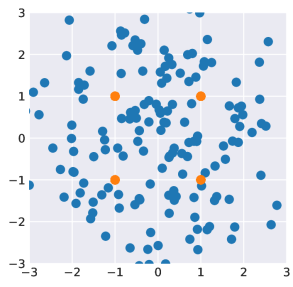
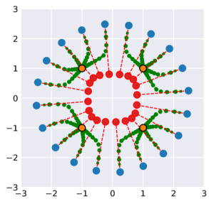
(a)

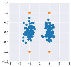
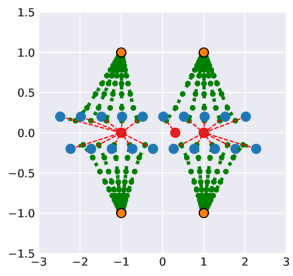
(b)

Figure 1: 2D Toy Example. Estimation of conditional mean and iterated estimation for points from a multimodal (4 modes) distribution under: (a) Denoising strong Gaussian noise (${\bm{H}}={\bm{I}}$); and (b) missing information recovery, i.e., ${\bm{H}}=[1,0;0,0]$, under moderate noise. Blue points represent observed samples, while red ones are the regression prediction. The black (hollow) circles represent the final point in our iterative procedure, always reaching a valid point in the data manifold (orange points). The small green circles indicate the iterative restoration path.

A Toy Example:

Let us assume we observe noisy samples ${\bm{y}}={\bm{H}}{\bm{x}}+{\bm{n}}$, where ${\bm{n}}~{}\sim\mathcal{N}(0,\sigma^{2}Id)$, drawn from a discrete multimodal distribution $p({\bm{x}})=\sum_{i=1}^{d}w_{i}\delta_{{\bm{x}}-{\bm{c}}_{i}}$, where ${\bm{c}}_{i}\in\mathbb{R}^{N}$ and $w_{i}\geq 0$ and $\sum_{i=1}^{d}w_{i}=1$.

Let ${\bm{x}}_{t}$ be the intermediate degraded samples according to equation 1. In this simple example, there is a closed form expression for all posterior distributions and conditional means; namely,

$$p({\bm{x}}_{t}|{\bm{x}})=G\left(\frac{{\bm{x}}_{t}-{\bm{H}}_{t}{\bm{x}}}{\sigma_{t}}\right)\quad\text{and}\quad p({\bm{x}}_{t})=\sum_{i=1}^{d}w_{i}G\left(\frac{{\bm{x}}_{t}-{\bm{H}}_{t}{\bm{c}}_{i}}{\sigma_{t}}\right),$$ (3)

where ${\bm{H}}_{t}=(1-t){\bm{I}}+t{\bm{H}}$ and $G({\bm{x}})$ is a Gaussian kernel with identity covariance and $\sigma_{t}=t\sigma$. Then,

$$\mathbb{E}_{{\bm{x}}\sim p({\bm{x}}|{\bm{x}}_{t})}[{\bm{x}}]=\int\frac{p({\bm{x}}_{t}|{\bm{x}})p({\bm{x}})}{p({\bm{x}}_{t})}{\bm{x}}d{\bm{x}}=\frac{\sum_{i=1}^{d}{\bm{c}}_{i}w_{i}G\left(\frac{{\bm{x}}_{t}-{\bm{H}}_{t}{\bm{c}}_{i}}{\sigma_{t}}\right)}{\sum_{i=1}^{d}w_{i}G\left(\frac{{\bm{x}}_{t}-{\bm{H}}_{t}{\bm{c}}_{i}}{\sigma_{t}}\right)}$$

The iteration from equation 2 becomes:

$$\hat{{\bm{x}}}_{t-\delta}=\frac{\delta}{t}\frac{\sum_{i=1}^{d}{\bm{c}}_{i}w_{i}G\left(\frac{\hat{\bm{x}}_{t}-{\bm{H}}_{t}{\bm{c}}_{i}}{\sigma_{t}}\right)}{\sum_{i=1}^{d}w_{i}G\left(\frac{\hat{\bm{x}}_{t}-{\bm{H}}_{t}{\bm{c}}_{i}}{\sigma_{t}}\right)}+\left(1-\frac{\delta}{t}\right)\hat{{\bm{x}}}_{t}.$$

Figure 1 shows the results of applying the iterative regression scheme given by the above equation in two different examples. The iterative regression converges to one of the four possible modes (shown in orange), while the regression to the mean is always a weighted average of all possible modes (i.e., a blurry reconstruction, shown in red).

Training and Inference: InDI ideal iterative scheme given by equation 2 requires to compute an estimate of the clean image at every step $t$ (i.e., $\mathbb{E}[\,{\bm{x}}_{0}\!\mid\!{\bm{x}}_{t}\,]$). To that extent, we train a family of regressors $F_{\theta}(\cdot;t)$, each of them specialized in reconstructing ${\bm{x}}_{0}$ from ${\bm{x}}_{t}$ at a given $t$. That is,

$$\min_{\theta}\mathbb{E}_{{\bm{x}},{\bm{y}}\sim p({\bm{x}},{\bm{y}})}\mathbb{E}_{t\sim p(t)}\|F_{\theta}({\bm{x}}_{t},t)-{\bm{x}}\|_{p},$$ (4)

where $p(t)$ is a predefined distribution for $t$ (e.g., uniform). The model $F_{\theta}$ allows us to do incremental reconstruction where from time step $t$ we predict the slightly less corrupted signal at time $t-\delta$ as given in equation 2. Thus, the iterative scheme becomes:

$$\hat{\bm{x}}_{t-\delta} =\frac{\delta}{t}F_{\theta}(\hat{\bm{x}}_{t},t)+\left(1-\frac{\delta}{t}\right)\hat{\bm{x}}_{t},$$ (5)

where $0<\delta\leq 1$. Although $\delta$ could be a function of time, in practice we use a constant time step, $\delta=\frac{1}{N}$, where $N$ is the number of steps.

InDI as a Residual Flow ODE:

In the limit, as $\delta\to 0$, equation 5 leads to an ordinary differential equation (ODE); namely

$$\frac{d{\bm{x}}_{t}}{dt}=\lim_{\delta\to 0}\frac{{\bm{x}}_{t}-{\bm{x}}_{t-\delta}}{\delta}=\frac{{\bm{x}}_{t}-F_{\theta}({\bm{x}}_{t},t)}{t},$$ (6)

where in the ideal case $F_{\theta}({\bm{x}}_{t},t)=\mathbb{E}[\,{\bm{x}}_{0}\!\mid\!{\bm{x}}_{t}\,]$. The ODE can be interpreted as a “residual flow” because the right-hand side is the (normalized) residual of the inversion process at time $t$. We are interested in the solution of this equation at $t=0$, starting from the initial condition ${\bm{x}}_{1}={\bm{y}}$ at $t=1$. The residual flow formulation can be used to develop other numerical procedures using standard ODE solvers. Exploring this is left to future work.

Another use of the continuous formulation is to understand the behavior of the proposed iterative procedure in terms of concrete examples. In Appendix B we show how the residual flow can be used to analyze the specific case where the prior is Gaussian and the restoration task is denoising.

Connection to Denoising Score-Matching and Probabilistic ODE:

An interesting connection emerges when the degradation is Gaussian noise (standard deviation $\sigma^{2}$). In this case, InDI’s ODE in equation 6 boils down to the score-matching probabilistic ODE of Song et al. (2021b). More specifically, let ${\bm{x}}_{t}={\bm{x}}+t{\bm{n}}$, so the noise level in ${\bm{x}}_{t}$ is $\sigma^{2}_{t}=t^{2}\sigma^{2}$. The probabilistic flow ODE (Eq(13) in Song et al. (2021b)) is given by

$$\frac{d{\bm{x}}_{t}}{dt}=-\frac{1}{2}\frac{d(\sigma_{t}^{2})}{dt}\nabla_{{\bm{x}}_{t}}\log p_{t}({\bm{x}}_{t})=-t\sigma^{2}\nabla_{{\bm{x}}_{t}}\log p_{t}({\bm{x}}_{t}).$$

According to the denoising score-matching (DSM) approximation (Vincent (2011)),

$$-\nabla_{{\bm{x}}_{t}}\log p_{t}({\bm{x}}_{t})\approx\frac{{\bm{x}}_{t}-F_{\theta}({\bm{x}}_{t},t)}{\sigma^{2}_{t}}=\frac{{\bm{x}}_{t}-F_{\theta}({\bm{x}}_{t},t)}{t^{2}\sigma^{2}},$$

so we end up recovering precisely the same ODE as in InDI. Furthermore, when $F_{\theta}({\bm{x}}_{t},t)=\mathbb{E}[\,{\bm{x}}_{0}\!\mid\!{\bm{x}}_{t}\,]$ (i.e., MMSE estimator) the DSM approximation is exact and the relation is given by Tweedie’s formula (Robbins, 1956; Efron, 2011).

Stochastic Perturbation: To make sure we have the regularity requirements for the iterative procedure from equation 2 to be well defined (Remark 4.2), we add a small amount of white noise to the low-quality input. As shown in Section 5 this leads to a significant improvement in image quality in certain tasks (in particular those that are restorations from deterministic degradations).

Our model with this noise perturbation becomes:

$${\bm{x}}_{t}=(1-t){\bm{x}}+t{\bm{y}}^{\prime}=(1-t){\bm{x}}+t{\bm{y}}+t\epsilon{\bm{n}}\quad\text{with}\,\,t\in[0,1],$$ (7)

where ${\bm{y}}^{\prime}={\bm{y}}+\epsilon{\bm{n}}$, $\epsilon$ is a small constant (e.g., $\epsilon=0.01$, where image values are in $[-1,1]$), and ${\bm{n}}\sim\mathcal{N}(0,Id)$.

A slightly more general formulation incorporates the perturbation as a general Brownian motion, where we can explicitly control the level of noise at each step. That is,

$${\bm{x}}_{t}=(1-t){\bm{x}}+t{\bm{y}}+\sqrt{t}\epsilon_{t}{\bm{\eta}}_{t}\quad\text{with}\,\,t\in[0,1],$$ (8)

where $\epsilon_{t}$ is a non-negative function, and ${\bm{\eta}}_{t}$ is the standard Brownian motion having zero mean and covariance $t{\bm{I}}$ at index $t$.

In this more general setting, the base training objective becomes

$$\min_{\theta}\mathbb{E}_{{\bm{x}},{\bm{y}}\sim p({\bm{x}},{\bm{y}})}\mathbb{E}_{t\sim p(t)}\mathbb{E}_{{\bm{n}}\sim\mathcal{N}(0,Id)}\left\|F_{\theta}\left((1-t){\bm{x}}+t{\bm{y}}+t\epsilon_{t}{\bm{n}};t\right)-{\bm{x}}\right\|_{p}.$$ (9)

And as a result, the general inference procedure in equation 2 becomes:

$$\hat{\bm{x}}_{t-\delta} =\frac{\delta}{t}F_{\theta}(\hat{\bm{x}}_{t},t)+\left(1-\frac{\delta}{t}\right)\hat{\bm{x}}_{t}+(t-\delta)\sqrt{\epsilon_{t-\delta}^{2}-\epsilon_{t}^{2}}{\bm{\zeta}},$$ (10)

where the reconstruction process starts from $t=1$, $\hat{\bm{x}}_{1}={\bm{y}}+\epsilon{\bm{n}}$ and ${\bm{n}}\sim\mathcal{N}(0,Id)$. At each step, a new ${\bm{\zeta}}\sim\mathcal{N}(0,Id)$ is sampled and noise is added to the current state. The added Gaussian noise is such that the noise at time $t$ has variance $t^{2}{\epsilon_{t}}^{2}$ as required by equation 8. To be well defined $\epsilon_{t}$ needs to be a non-negative non-increasing function of $t$. In the limit case where $\epsilon_{t}=\epsilon$ we are in the simplified case given by equation 7, while if $\epsilon_{t}=\frac{\epsilon}{\sqrt{t}}$ the noise perturbation is a pure Brownian motion.

Our full iterative restoration inference scheme is given in Algorithm 1.

Algorithm 1 Iterative Image Restoration (Inference)

${\bm{y}},F_{\theta}(\cdot,t),\delta,\epsilon_{t}$

${\bm{n}}\sim\mathcal{N}({\bm{0}},{\bm{I}})$

$\hat{\bm{x}}_{1}={\bm{y}}+\epsilon_{1}{\bm{n}}$

for $t=1\ \mathrm{\mathbf{to}}\ 0\,\,\mathrm{\mathbf{with\,\,step}}\ \mathrm{-\delta}$ do

     ${\bm{\zeta}}\sim\mathcal{N}({\bm{0}},{\bm{I}})$

     $\hat{\bm{x}}_{t-\delta}\leftarrow\frac{\delta}{t}F_{\theta}(\hat{\bm{x}}_{t},t)+\left(1-\frac{\delta}{t}\right)\hat{\bm{x}}_{t}+(t-\delta)\sqrt{\epsilon_{t-\delta}^{2}-\epsilon_{t}^{2}}{\bm{\zeta}}$ $\triangleright$ Update rule from equation 10.

end for

return $\hat{\bm{x}}_{0}$

5 Experiments

We train and evaluate our framework on four widely popular image restoration tasks: motion deblurring, defocus deblurring, compression artifacts removal and single image super-resolution. Our formulation is generative-based, and we show that can be used for image generation even if this is not the main focus of the present work. To evaluate the quality of the proposed method we compute several distortion based and perceptual metrics: PSNR, LPIPS (Zhang et al., 2018), FID (Fréchet Inception Distance) (Heusel et al., 2017), and KID (Kernel Inception Distance) (Bińkowski et al., 2018).

Perception–Distortion tradeoff (Blau & Michaeli, 2018): To illustrate the potential of the method, we present results when using different number of steps for the reconstruction. This has a direct impact on the perception–distortion tradeoff. In general, a single step reconstruction with our model, will lead to an estimate that minimizes the average point distortion (e.g., PSNR) but this can be only done to the detriment of the perceptual quality.

Model Architecture and Training: We adopt a U-Net-like architecture similar to the ones in diffusion strategies (Saharia et al., 2021; Whang et al., 2022). Following Whang et al. (2022) we removed attention layers and group normalization to have a fully-convolutional architecture. The size of the model varies for each evaluated task (in general we chose a model size proportional to the size of the dataset to avoid significant overfitting). The model is trained on image crops using ADAM optimizer. Learning rates and other hyper-parameters are given in Appendix C. For each experiment, we train a single model $F_{\theta}(\cdot;t)$ that is conditioned on the parameter $t$. The model is trained using the loss function of equation 9 with $p=1$. We found that the distribution of $t$, $p(t)$ plays an important role. In Section 6.3 we present an empirical analysis of its impact.

5.1 Motion Deblurring

Motion deblurring is a very challenging restoration task. Motion is intrinsically random in the sense that a priori we don’t have a known degradation model. The current best end-to-end deep learning solution is to train regression models using paired data sharp, blurry frames. One of the most adopted training datasets is the GoPro motion deblurring dataset (Nah et al., 2017) containing 3214 pairs of clean and blurry $1280\times 720$ images ($1111$ are reserved for evaluation). The blurry frames are generated by recording high-frame rate video clips and then averaging consecutive frames to simulate blurs caused due to longer exposure. We follow the standard setup (Nah et al., 2017; Kupyn et al., 2019; Chen et al., 2021a; Cho et al., 2021; Suin et al., 2020; Zhang et al., 2019) and perform training data augmentation with random horizontal/vertical flips and 90/180/270 rotations. We did not introduce additional noise to the blurry inputs ($\epsilon=0$ in equation 7).

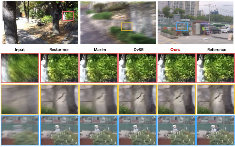
Figure 2: Examples of deblurred images from GoPro dataset. Our iterative reconstruction leads achieves better reconstruction of detailed textures than regression based models (Restormer, Maxim) and similar quality than conditional DPMs (DvSR). More results are provided in Appendix.

Table 1: Image motion deblurring on the GoPro (Nah et al., 2017) dataset. Best values and second-best values for each metric are color-coded. KID values are scaled by a factor of 1000 for readability.

	Perceptual				Distortion
	LPIPS$\downarrow$	NIQE$\downarrow$	FID$\downarrow$	KID$\downarrow$	PSNR$\uparrow$	SSIM$\uparrow$
Ground Truth	0.0	3.21	0.0	0.0	$\infty$	1.000
HINet (Chen et al., 2021a)	0.088	4.01	17.91	8.15	32.77	0.960
MPRNet (Zamir et al., 2021)	0.089	4.09	20.18	9.10	32.66	0.959
MIMO-UNet+ (Cho et al., 2021)	0.091	4.03	18.05	8.17	32.45	0.957
SAPHNet (Suin et al., 2020)	0.101	3.99	19.06	8.48	31.89	0.953
DeblurGANv2 (Kupyn et al., 2019)	0.117	3.68	13.40	4.41	29.08	0.918
DvSR (Whang et al., 2022)	0.059	3.39	4.04	0.98	31.66	0.948
DvSR-SA (Whang et al., 2022)	0.078	4.07	17.46	8.03	33.23	0.963
Restormer (Zamir et al., 2022)	0.084	4.11	19.33	8.78	32.92	0.961
MAXIM (Tu et al., 2022)	0.087	3.94	22.76	10.06	32.86	0.962
NAFNet (Chen et al., 2022)	0.078	4.07	17.87	8.27	33.71	0.967
Ours (10 steps)	0.058	3.32	3.55	0.56	31.49	0.946

Figure 2 shows a visual comparison of our iterative image restoration and current state-of-the-art deblurring models. The iterative scheme produces images with much more details than regression based solutions (Restormer (Zamir et al., 2022), MAXIM (Tu et al., 2022)). Our results are similar to the ones generated by current conditional diffusion models (DvSR (Whang et al., 2022)). Quantitative results on the GoPro dataset are presented in Table 1. The proposed iterative reconstruction procedure achieves a new state-of-the-art performance across perceptual metrics while maintaining competitive PSNR to existing methods.

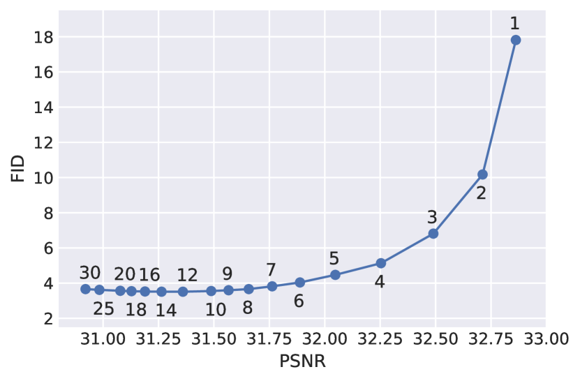
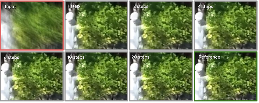
Figure 3: Number of steps. The total number of steps in the iterative regression has a direct impact on the quality. The number of steps seems to control the Perception-distortion tradeoff. One step leads to the best possible MSE reconstruction (minimum distortion) but large perceptual discrepancy.

Number of steps. Figure 3 shows the impact of the number of inference steps on the Perception–Distortion trade-off (Blau & Michaeli, 2018). While doing a reconstruction on a single step (e.g., direct regression) produces the best PSNR, the perceptual metrics are significantly improved when the number of steps is larger than one. Both metrics can’t be optimized simultaneously (Blau & Michaeli, 2018).

5.2 Single-Image Super-resolution

We evaluated the iterative restoration methodology on single-image $4\times$ super-resolution on the div2k dataset (Agustsson & Timofte, 2017). This dataset contains 1000 2K-resolution images (800 for training, 100 images for validation, 100 testing). We compare to other state-of-the art models that span from regression models having powerful architectures (Wang et al., 2018; Chen et al., 2021b; Liang et al., 2022) and/or generative formulations: GAN based, i.e., LDL (Liang et al., 2022), ESRGAN (Wang et al., 2018), BSRGAN (Zhang et al., 2021); and also based on Normalizing Flows, SRFLOW (Lugmayr et al., 2020).

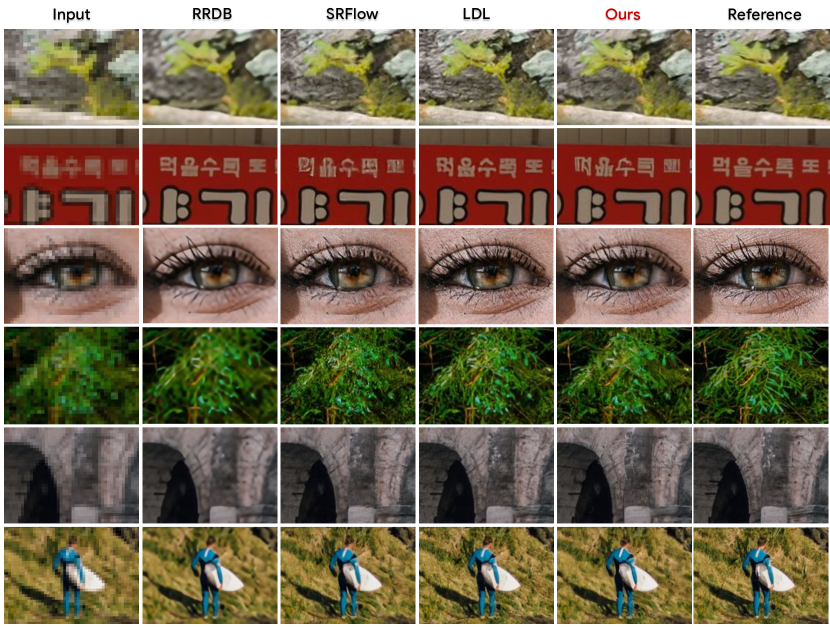
Figure 4: Examples image $4\times$ upscaling. Our iterative reconstruction leads achieves better reconstruction of detailed textures than RRDB regression model (Wang et al., 2018), less high-frequency artifacts than SRFlow (Lugmayr et al., 2020) generative normalizing flow, and comparable visual quality than LDL (Liang et al., 2022) a state-of-the-art customized generative adversarial model. More results are given in Appendix.

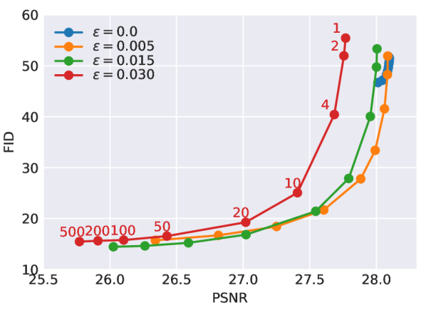
(a)

	Type	PSNR$\uparrow$	LPIPS$\downarrow$	FID$\downarrow$	KID$\downarrow$
LDL(SwinIR) (Liang et al., 2022)	GAN	26.64	0.102	10.80	0.400
LDL(RRDB) (Liang et al., 2022)	GAN	26.43	0.109	11.36	0.582
ESRGAN (Wang et al., 2018)	GAN	25.54	0.125	12.77	0.732
SRFLOW (Lugmayr et al., 2020)	NF	26.10	0.127	20.21	4.444
BSRGAN (Zhang et al., 2021)	GAN	24.35	0.241	31.43	5.229
RRDB (Wang et al., 2018)	REG	28.37	0.264	50.98	19.000
LIIF (Chen et al., 2021b)	REG	28.15	0.269	53.16	19.958
BSRNET (Zhang et al., 2021)	REG	25.90	0.348	84.11	36.901
Ours (100 steps, $\epsilon=0.015$)		26.45	0.136	15.39	1.761

(b)

Figure 5: $4\times$ Super-resolution on div2k dataset (Agustsson & Timofte, 2017). Best values and second-best values for each metric are color-coded

Figure 5(b) summarizes the quantitative results on $4\times$ SR div2k validation dataset. Figure 4 shows a selection of results. Our proposed framework leads to upscaled images with more defined structure than regression based formulations producing larger PSNR, e.g., RRDB (Wang et al., 2018). The recently introduced adversarial formulation LDL (Liang et al., 2022) produces slightly better fine grain details. This could indicate that in the situation where there is limited training data, careful adversarial formulation may be more data efficient.

The importance of adding noise in deterministic super-resolution. In our formulation of super-resolution, the degradation is a deterministic linear (blurring plus subsampling) operator. Figure 5(a) shows the importance of adding a small amount of noise to the input image. Directly applying the original iterative procedure (without adding noise to the input) leads to a blurry reconstruction (high PSNR but low FID score, $\epsilon=0.0$ in Figure 5 (a)). Adding a small amount of noise ($\epsilon>0$ in Figure 5(a)) leads to significant better results in terms of perceptual quality (e.g., FID score).

5.3 Defocus deblurring

Defocus deblurring is the task of reducing the blur due to limited depth-of-field or misfocus. For such purposes we used the Canon dual-pixel (DP) defocus dataset (DDPD) provided by Abuolaim & Brown (2020), and train a defocus deblurring model only using single image input (i.e., we don’t use the dual-pixel images given in the dataset). The DDPD dataset contains 1000 pairs of sharp and blurry $6720\times 4480$ images, of which 30% are reserved for validation and testing. The blurry/sharp frames are generated by capturing two consecutive snapshots by changing the camera parameters (lens aperture). high-frame rate video clips and then averaging consecutive frames to simulate blurs caused due to longer exposure.

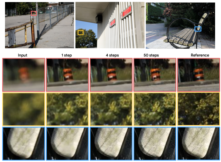
Figure 6: Examples of restored images from defocus DDPD dataset. The iterative reconstruction leads to images with more texture compared to the direct regression (1 step). More results are provided in Appendix.

Figure 6 shows a visual comparison of our iterative image restoration when a different number of inference steps is used. Increasing the number of steps has a direct impact on the quality of the result. Quantitative results on the DDPD dataset are summarized in Table 3 in Appendix. As in the other experiments the best PSNR is obtained with a single step (direct regression), while the best perceptual metrics are obtained when the restoration is done in multiple steps. We did not introduce additional noise to the blurry inputs ($\epsilon=0$ in equation 7).

5.4 Compression artifact removal

JPEG compression introduces blocking artifacts and lack of high-frequency details. We evaluated the proposed method on the task of removing strong JPEG compression artifacts (quality factor 15). To generate the training data we use the 1000 div2k high-quality images (Agustsson & Timofte, 2017). We evaluated the model on div2k validation set.

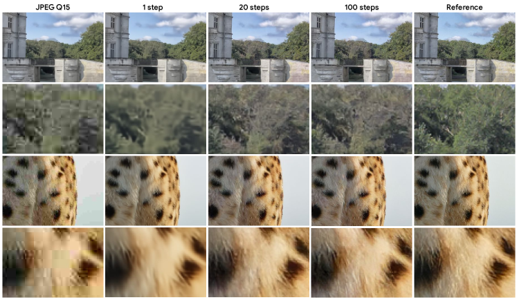
Figure 7: JPEG Compression artifacts removal (quality factor 15). As more inference steps are used more details are generated.

Figure 7 show some visual results of restored images with the model applying a different number of steps. As more inference steps are used the restored images have more details. More results on JPEG compression removal are discussed in the next section.

6 Discussion

6.1 A generative framework

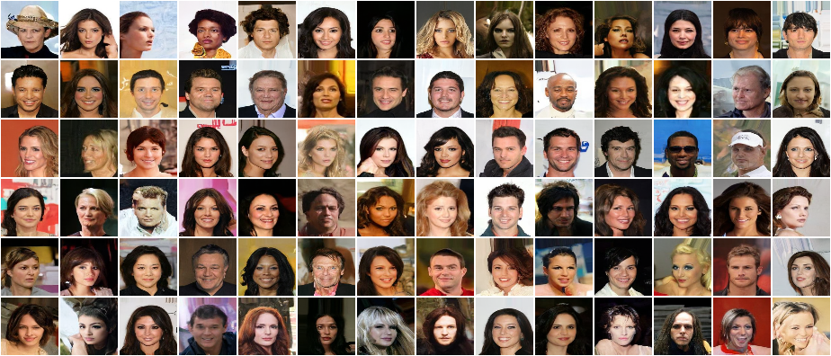
Figure 8: Examples of CelebA $64\times 64$ generated samples (FID=$9.19$, 150 steps). Our iterative reconstruction can be potentially used to generated samples from a fully-degraded image (noise).

A natural question to ask is whether the proposed approach is also generative in the spirit of diffusion formulations. Namely, if we take our formulation to the limit where the low-quality image is fully degraded, then could we potentially generate new samples from scratch?

To test the idea we trained a restoration model that starts from pure Gaussian noise paired to a $64\times 64$ celebA image and then proceed as described above. Figure 8 shows some generated samples with this formulation. The generated samples have a FID=9.19, which is not state-of-the-art but illustrate the point. In this specific case, our proposed methodology leads to a similar denoising training loss as the one in DDPM (Ho et al., 2020). Despite this similarity, the two methods come from different motivations/formulations and therefore have different inference strategies. We didn’t fine-tune architecture or hyper-parameters to boost the performance since our goal was to present the idea and show that the formulation, at its core, can be generative as well.

6.2 Comparison of Inference Algorithms

In what follows we discuss different alternatives for recovering the clean sample with the trained models.

Naive Procedure and Relevance to Cold Diffusion: Given equation 1, one may be tempted to directly replace the clean image by the current estimate. This would lead to $\hat{{\bm{x}}}_{t}=(1-t)F_{\theta}(\hat{\bm{x}}_{s},t)+t{\bm{y}}$, and the inference iterative rule would become

$$\hat{\bm{x}}_{t-\delta} =(1-t+\delta)F_{\theta}(\hat{\bm{x}}_{t},t)+(t-\delta){\bm{y}}.$$ (11)

Cold Diffusion (Bansal et al., 2022) proposes to generate images by inverting an arbitrary known degradation $D({\bm{x}},s)$, where $s$ controls the strength. Our formulation is more general in the sense that we don’t require an explicit knowledge of $D$. To apply Cold Diffusion sampling in our context, we define $D({\bm{x}},s)=(1-s){\bm{x}}+s{\bm{y}}$ (given by equation 1). This leads to Cold Diffusion’s naive sampling (Algorithm 1 in Bansal et al. (2022)),

$$\hat{\bm{x}}_{t-\delta} =D(F_{\theta}(\hat{\bm{x}}_{t},t),t-\delta)=(1-t+\delta)F_{\theta}(\hat{\bm{x}}_{t},t)+(t-\delta){\bm{y}}.$$ (12)

Note that this sampling scheme is the same as the one in Eq. 11. Cold diffusion improved sampling (Algorithm 2 in Bansal et al. (2022)) is given by,

$$\hat{\bm{x}}_{t-\delta} =\hat{\bm{x}}_{t}-D(F_{\theta}(\hat{\bm{x}}_{t},t),t)+D(F_{\theta}(\hat{\bm{x}}_{t},t),t-\delta)$$ (13)

$$=\hat{\bm{x}}_{t}-(1-t)F_{\theta}(\hat{\bm{x}}_{t},t)-t{\bm{y}}+(1-t+\delta)F_{\theta}(\hat{\bm{x}}_{t},t)+(t-\delta){\bm{y}}$$ (14)

$$=\hat{\bm{x}}_{t}+\delta(F_{\theta}(\hat{\bm{x}}_{t},t)-{\bm{y}}).$$ (15)

In Figure 9 we compare our inference algorithm (equation 5), the naive inference algorithm (equation 11), and our adaptation of the Cold Diffusion sampler to our formulation (equation 15). In general, the naive sampler produces good results with very few steps (N=2,3) but then diverges. Our adaptation of Cold Diffusion sampler produces competitive results, while leading to slightly worse FID scores for the same distortion level than our proposed algorithm. In the limit, as the number of steps becomes very large, Cold Diffusion sampler seems to converge to a stable point, while ours after a certain large number of steps, deteriorates.

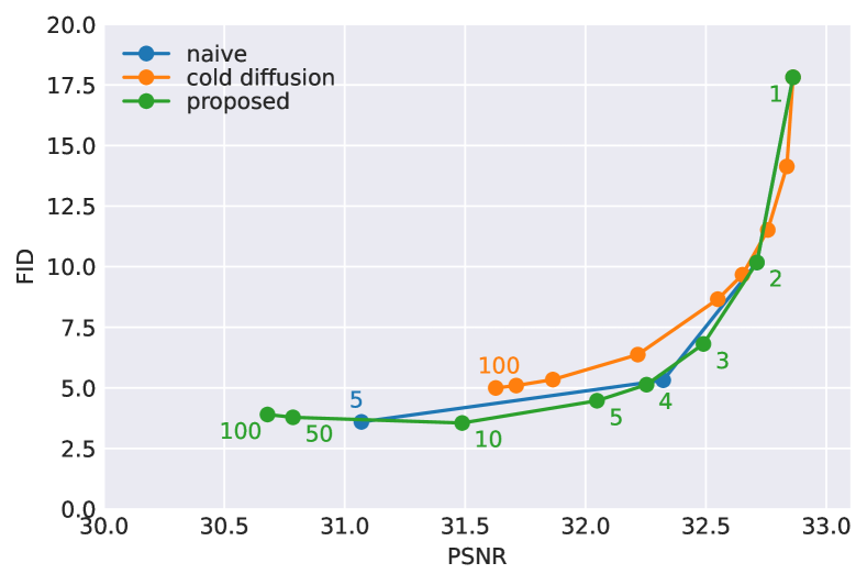
(a) Motion Deblurring (GoPro dataset)

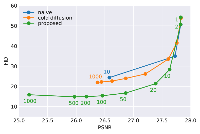
(b) Upscaling $4\times$ (div2k dataset)

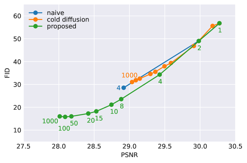
(c) De-Jpeg Q15 (div2k dataset)

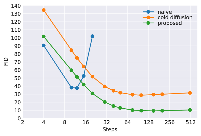
(d) Generative imaging CelebA $64\times 64$

Figure 9: Impact of the Inference Algorithm for some of the different tested tasks. The naive inference algorithm (equation 11) produces a good baseline when used with very few steps (i.e. 2–5) but then diverges. The proposed updated rule (equation 5) produces better results than the one adapted from Cold Diffusion (Bansal et al., 2022) given in (equation 15). At very large number of steps, Cold Diffusion seems to be the most stable of the three tested samplers. Each of the points in each shown curve represents the results with a different number of steps (similar to what is shown in Figure  3. Points that leads to values that are out-of-the shown region are left out for improving visualization.

Figure 9. shows the FID score of CelebA 64x64 generated images when using the three different variants of the inference algorithm (sampler).

6.3 Impact of distribution p(t)

key	$p(t)$	description
‘linear_0’	$t\sim\mathcal{U}[0,1]$	Uniform distribution
‘linear_a’	$t\sim\frac{1}{1+a}\mathcal{U}[0,1]+\frac{a}{1+a}\delta_{1}$, where $a\geq 0$	Uniform distribution w/bias to $t=1$
‘bias_t1’	$t=g(s)$, $s\sim\mathcal{U}[0,1]$ and $g(s)=\sin\left(s\pi/2)\right)$	Sine based distribution (bias to $t=1$)
‘bias_t0’	$t=g(s)$, $s\sim\mathcal{U}[0,1]$ and $g(s)=\sin\left((s-1)\pi/2)\right)+1$	Sine based distribution (bias to $t=0$)
‘bias_t0_t1’	$t=g(s)$, with $s\sim\mathcal{U}[0,1]$ and $g(s)=\sin\left(s\pi/2)\right)^{2}$	Sine based distribution (bias to $t=1$)

(a) Different evaluated $p(t)$ training distributions.

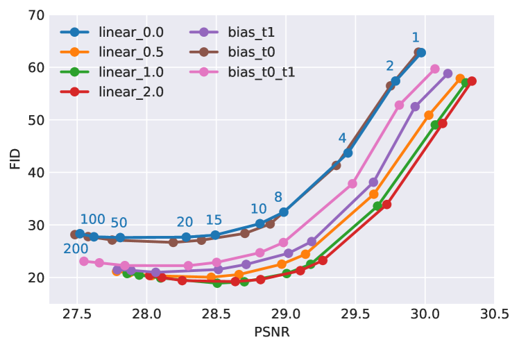
(b) PSNR vs FID plot for different $p(t)$.

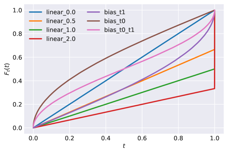
(c) Visualization of $p(t)$ cumulative distributions.

Figure 10: Impact of the distribution of $p(t)$ during training. Results for JPEG Compression removal (Q=15). The best results are obtained when the distribution of $t$ is biased towards $t=1$.

The impact of the distribution of $t$ used during training has a clear impact on performance. We evaluated several different options that are summarized in Figure 10 (a). Figure 10 (b) shows the results when different distributions are adopted. The best results are obtained when the model is trained with a bias towards $t=1$ (more degradation). Intuitively, this could imply that the iterative procedure needs to be more certain of the direction to move at the very early steps of the procedure. Nonetheless, the best distribution can depend on a combination of model capacity and restoration task so we are not drawing general conclusions.

6.4 Impact of adding noise on inverting deterministic degradations

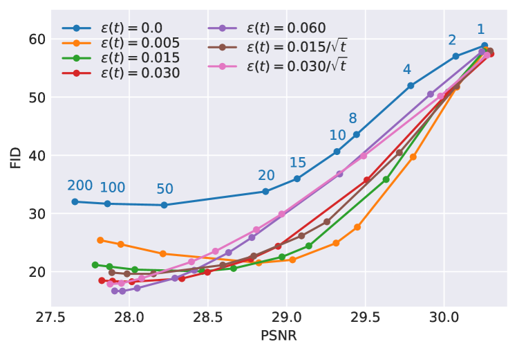
(a)

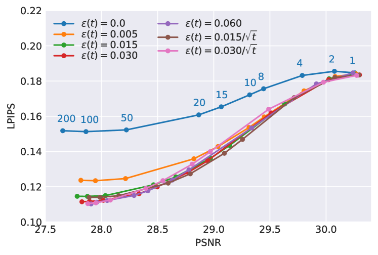
(b)

Figure 11: Impact of adding noise to the low-quality input in JPEG compression removal.

JPEG compression is a non-linear, but deterministic, degradation. We empirically verified that adding a small amount of noise helps to improve the results as shown in Figure 11. We tested the variant of the inference algorithm that adds noise at each step (so the noise becomes a Brownian motion, e.g., $\epsilon_{t}=\epsilon/\sqrt{t}$), and adding a constant noise level at the initial step ($\epsilon_{t}=\epsilon$). We did not observe any practical difference in the two approaches.

6.5 Comparison to a Conditional Denoising Diffusion Model

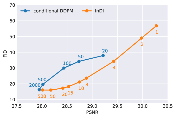
(b) PSNR vs FID.

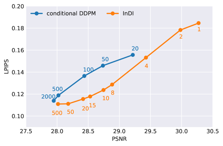
(c) PSNR vs LPIPS.

Figure 12: Comparison of InDI to a conditional Denoising Diffusion Probabilistic Model (DDPM). The DDPM requires a noise schedule for inference. The plot showed herein was built by fusioning six different noise schedules taking the best PSNR vs FID score at a given number of steps. Our proposed InDI algorithm produces comparable results in much less number of steps.

We compare InDI to a vanilla conditional DDPM (Ho et al., 2020). We trained a vanilla conditional DDPM, using the (continuous) noise level as an additional input, similarly as done in Saharia et al. (2021); Whang et al. (2022). The model architecture is the same as in InDI but the auxiliary noise image (needed in any DDPM) is concatenated with the low-quality input at each step. Figure 12 shows a comparison between InDI and the conditional DDPM. To generate the DDPM plot we merged several possible noise schedules using different number of steps that span the perception-distortion tradeoff. InDI produces comparable results using significant less number of steps than the vanilla DDPM.

7 Conclusions and Limitations

We presented a novel formulation of image restoration that circumvents the regression-to-the mean problem. This allows us to get restored images with superior realism and perceptual quality, while still having a low distortion error. Our method is motivated by the observation that restoration from a small distortion is a better-conditioned problem. We therefore break a restoration task into many small ones – each of them easier (and less ill-posed) than the larger problem we solve overall. This enables our iterative approach to transforming the degraded image into a high-quality image, in spirit similar to current generative diffusion models.

Limitations. The present formulation is a supervised one, requiring paired training data. As such, for each type of degradation we need to train a specialized model, in contrast to unsupervised formulations such as RED (Romano et al., 2017), PnP (Venkatakrishnan et al., 2013; Kamilov et al., 2022), or DDRM (Kawar et al., 2022). Additionally, given the dependence to paired training data, its performance for out-of-distribution samples is not guaranteed. This question requires more in-depth analysis. Finally, while the proposed iterative inference algorithm produces high-quality restorations, in some tasks performance degrades after a certain number of steps. This is likely due to the accumulation of errors, and will likely require a more robust inference scheme.

For future work, we would like to better characterize the limiting points of the proposed inference procedure. Other possible research avenues are developing robust formulations that can successfully handle out-of-domain input.

Acknowledgments

The authors would like to thank our colleagues Jon Barron, Tim Salimans, Jascha Sohl-dickstein, Ben Poole, José Lezama, Sergey Ioffe, and Jason Baldridge for helpful discussions.

Appendix A Proof of Proposition 4.1

Proof.

We have ${\bm{x}}_{s}=(1-s){\bm{x}}+s{\bm{y}}$, and ${\bm{x}}_{t}=(1-t){\bm{x}}+t{\bm{y}}$, so by substituting ${\bm{y}}$ from one to the other we get,

$${\bm{x}}_{s} =(1-s){\bm{x}}+s\left(\frac{{\bm{x}}_{t}-(1-t){\bm{x}}}{t}\right)$$ (16)

$$={\bm{x}}-s{\bm{x}}+\frac{s}{t}{\bm{x}}_{t}-\frac{s}{t}{\bm{x}}+s{\bm{x}}$$ (17)

$$=\left(1-\frac{s}{t}\right){\bm{x}}+\frac{s}{t}{\bm{x}}_{t}.$$ (18)

Then,

$$\mathbb{E}[\,{\bm{x}}_{s}\!\mid\!{\bm{x}}_{t}\,] =\int{\bm{x}}_{s}p_{{\bm{x}}_{s}|{\bm{x}}_{t}}({\bm{x}}_{s}|{\bm{x}}_{t})d{\bm{x}}_{s}$$ (19)

$$=\int{\bm{x}}_{s}p_{{\bm{x}}|{\bm{x}}_{t}}\left(\frac{t{\bm{x}}_{s}-s{\bm{x}}_{t}}{t-s}\Big{|}{\bm{x}}_{t}\right)\frac{t}{t-s}d{\bm{x}}_{s}$$ (20)

$$=\int\frac{(t-s){\bm{x}}+s{\bm{x}}_{t}}{t}p_{{\bm{x}}|{\bm{x}}_{t}}({\bm{x}}|{\bm{x}}_{t})d{\bm{x}}$$ (21)

$$=\left(1-\frac{s}{t}\right)\int{\bm{x}}p_{{\bm{x}}|{\bm{x}}_{t}}({\bm{x}}|{\bm{x}}_{t})d{\bm{x}}+\frac{s}{t}{\bm{x}}_{t}$$ (22)

$$=\left(1-\frac{s}{t}\right)\mathbb{E}[\,{\bm{x}}\!\mid\!{\bm{x}}_{t}\,]+\frac{s}{t}{\bm{x}}_{t}.$$ (23)

where we have applied the fact that $p_{{\bm{x}}_{s}|{\bm{x}}_{t}}({\bm{x}}_{s}|{\bm{x}}_{t})=p_{{\bm{x}}|{\bm{x}}_{t}}({\bm{x}}|{\bm{x}}_{t})\frac{t}{t-s}$ and ${\bm{x}}=\frac{t{\bm{x}}_{s}-s{\bm{x}}_{t}}{t-s}$. ∎

Appendix B Denoising with a Gaussian Prior

Let’s analyze InDI’s behavior in the particular case where $p(\textbf{x})=N(\textbf{c},\sigma^{2}_{c}\textbf{I})$, and the restoration task is denoising $\textbf{y}=\textbf{x}+\textbf{n}$, where n is white Gaussian of fixed standard deviation $\sigma_{N}$. Then, $p(\textbf{y}|\textbf{x})=N(\textbf{x},\sigma^{2}_{N}\textbf{I})$ and $\mathbb{E}[\textbf{x}|\textbf{x}_{t}]=\frac{\sigma^{2}_{c}\textbf{x}_{t}+t^{2}\sigma^{2}_{N}\textbf{c}}{\sigma^{2}_{c}+t^{2}\sigma^{2}_{N}}$, where we have used the fact that $\textbf{x}_{t}=(1-t)\textbf{x}+t\textbf{y}=\textbf{x}+t\textbf{n}$.

InDI’s ideal ODE is given by $\frac{d\textbf{x}_{t}}{dt}=\frac{\textbf{x}_{t}-\mathbb{E}[\textbf{x}|\textbf{x}_{t}]}{t},$ which in this case becomes:

$$\frac{d\textbf{x}_{t}}{dt}=\frac{t\sigma^{2}_{N}(\textbf{x}_{t}-\textbf{c})}{\sigma^{2}_{N}t^{2}+\sigma^{2}_{c}}.$$

We are interested in solving this equation at $t=0$, with boundary condition $\textbf{x}_{1}=\textbf{y}$ at $t=1$. This is a separable ODE having general solution: $\textbf{x}_{t}=\textbf{c}+(\textbf{y}-\textbf{c})\sqrt{\frac{t^{2}+\alpha^{2}}{1+\alpha^{2}}}$, where $\alpha=\frac{\sigma_{c}}{\sigma_{N}}$. The solution at $t=0$, is

$$\textbf{x}_{\text{InDI}}=\textbf{c}+(\textbf{y}-\textbf{c})\sqrt{\frac{\sigma^{2}_{c}}{\sigma^{2}_{c}+\sigma^{2}_{N}}}.$$

Note that $\mathbb{E}[\textbf{x}_{\text{InDI}}]=\textbf{c}=\mathbb{E}[\textbf{x}]$, and the covariance $\text{cov}(\textbf{x}_{\text{InDI}})=\text{cov}(\textbf{y})\frac{\sigma^{2}_{c}}{\sigma^{2}_{c}+\sigma^{2}_{N}}=\text{cov}(\textbf{x})$, since $\text{cov}(\textbf{y})=(\sigma^{2}_{c}+\sigma^{2}_{N})\textbf{I}.$ Given $p(\textbf{x})$ and $p(\textbf{x}_{\text{InDI}})$ are Gaussian distributions with same mean and covariance, we have $p(\textbf{x}_{\text{InDI}})=p(\textbf{x})$. That is, in the limit, InDI generates samples from the prior distribution $p(\textbf{x})$.

It is worth noting that in this case the MMSE and MAP estimates coincide,

$$\textbf{x}_{\text{MMSE}}=\textbf{x}_{\text{MAP}}=\frac{\sigma^{2}_{c}\textbf{y}+\sigma^{2}_{N}\textbf{c}}{\sigma^{2}_{c}+\sigma^{2}_{N}},$$

and are in fact different from InDI’s estimate.

Appendix C Model and Training Details

In all our restoration experiments we use a U-Net-like architecture (Ronneberger et al., 2015) similar to the one in SR3 (Saharia et al., 2021) and DvSR (Whang et al., 2022). We followed the same adaptations as the ones introduced in Whang et al. (2022) to make it fully-convolutional (removed self-attention layers and group normalization). Our U-Net has an adaptive number of resolutions each of them having an arbitrary number of channels (given by a multiplication factor from a base set of channels).

Table 2 summarizes the model definition for each of the tested applications.

Table 2: Model and training parameters for each restoration task.

	channels	multipliers	noise	$p(t)$	batch size	learning rate	crop size	# params.
motion deblurring	64	[1,2,3,4]	$\epsilon=0$	bias_t1	256	$10^{-4}$	$128\times 128$	27.68M
defocus deblurring	64	[1,2,4,4]	$\epsilon=0$	linear_0.5	1024	$10^{-4}$	$128\times 128$	33.57M
JPEG restoration	64	[1,2,4,4]	$\epsilon=0.060$	linear_1.0	1024	$10^{-4}$	$128\times 128$	33.57M
$4\times$ super-resolution	96	[1,2,3,4]	$\epsilon=0.015$	bias_t1	256	$10^{-4}$	$256\times 256$	62.25M

All models are trained for 500K steps using 32 TPUv3 cores. We used the Adam optimizer with a fixed learning rate, and EMA decay rate of 0.9999. Models were trained using the respective indicated distribution for $p(t)$. For the super-resolution model, low-resolution crops of size $64\times 64$ are upscaled using bilinear interpolation to $256\times 256$ before feeding them into the model.

Appendix D Additional Results

\begin{overpic}[width=433.62pt]{assets/appendix/gopro/input_GOPR0868_11_00-000071_crop1.png} \put(2.0,2.0){\color[rgb]{1,1,1}Input} \end{overpic}

\begin{overpic}[width=433.62pt]{assets/appendix/gopro/ref_GOPR0868_11_00-000071_crop1.png} \put(2.0,2.0){\color[rgb]{1,1,1}Reference} \end{overpic}

\begin{overpic}[width=433.62pt]{assets/appendix/gopro/s1_GOPR0868_11_00-000071_crop1.png} \put(2.0,2.0){\color[rgb]{1,1,1}1 step} \end{overpic}

\begin{overpic}[width=433.62pt]{assets/appendix/gopro/s4_GOPR0868_11_00-000071_crop1.png} \put(2.0,2.0){\color[rgb]{1,1,1}4 steps} \end{overpic}

\begin{overpic}[width=433.62pt]{assets/appendix/gopro/s10_GOPR0868_11_00-000071_crop1.png} \put(2.0,2.0){\color[rgb]{1,1,1}10 steps} \end{overpic}

\begin{overpic}[width=433.62pt]{assets/appendix/gopro/s20_GOPR0868_11_00-000071_crop1.png} \put(2.0,2.0){\color[rgb]{1,1,1}20 steps} \end{overpic}

Figure 13: Additional GoPro deblurring results. The proposed method (InDI) applied with different number of reconstruction steps. Best viewed electronically.

\begin{overpic}[width=433.62pt]{assets/appendix/gopro/input_GOPR0869_11_00-000087_crop3.png} \put(2.0,2.0){\color[rgb]{1,1,1}Input} \end{overpic}

\begin{overpic}[width=433.62pt]{assets/appendix/gopro/ref_GOPR0869_11_00-000087_crop3.png} \put(2.0,2.0){\color[rgb]{1,1,1}Reference} \end{overpic}

\begin{overpic}[width=433.62pt]{assets/appendix/gopro/s1_GOPR0869_11_00-000087_crop3.png} \put(2.0,2.0){\color[rgb]{1,1,1}1 step} \end{overpic}

\begin{overpic}[width=433.62pt]{assets/appendix/gopro/s4_GOPR0869_11_00-000087_crop3.png} \put(2.0,2.0){\color[rgb]{1,1,1}4 steps} \end{overpic}

\begin{overpic}[width=433.62pt]{assets/appendix/gopro/s10_GOPR0869_11_00-000087_crop3.png} \put(2.0,2.0){\color[rgb]{1,1,1}10 steps} \end{overpic}

\begin{overpic}[width=433.62pt]{assets/appendix/gopro/s20_GOPR0869_11_00-000087_crop3.png} \put(2.0,2.0){\color[rgb]{1,1,1}20 steps} \end{overpic}

Figure 14: Additional GoPro deblurring results. The proposed method (InDI) applied with different number of reconstruction steps. Best viewed electronically.

\begin{overpic}[width=433.62pt]{assets/appendix/gopro/input_GOPR0410_11_00-000142_crop2.png} \put(2.0,2.0){\color[rgb]{1,1,1}Input} \end{overpic}

\begin{overpic}[width=433.62pt]{assets/appendix/gopro/ref_GOPR0410_11_00-000142_crop2.png} \put(2.0,2.0){\color[rgb]{1,1,1}Reference} \end{overpic}

\begin{overpic}[width=433.62pt]{assets/appendix/gopro/s1_GOPR0410_11_00-000142_crop2.png} \put(2.0,2.0){\color[rgb]{1,1,1}1 step} \end{overpic}

\begin{overpic}[width=433.62pt]{assets/appendix/gopro/s4_GOPR0410_11_00-000142_crop2.png} \put(2.0,2.0){\color[rgb]{1,1,1}4 steps} \end{overpic}

\begin{overpic}[width=433.62pt]{assets/appendix/gopro/s10_GOPR0410_11_00-000142_crop2.png} \put(2.0,2.0){\color[rgb]{1,1,1}10 steps} \end{overpic}

\begin{overpic}[width=433.62pt]{assets/appendix/gopro/s20_GOPR0410_11_00-000142_crop2.png} \put(2.0,2.0){\color[rgb]{1,1,1}20 steps} \end{overpic}

Figure 15: Additional GoPro deblurring results. The proposed method (InDI) applied with different number of reconstruction steps. Best viewed electronically.

\begin{overpic}[width=214.63977pt]{assets/appendix/sisr_4x/input_0004_crop1_NN.png} \put(2.0,2.0){\color[rgb]{1,1,1}Input} \end{overpic}\begin{overpic}[width=214.63977pt]{assets/appendix/sisr_4x/ref_0004_crop1.jpg} \put(2.0,2.0){\color[rgb]{1,1,1}Reference} \end{overpic}

\begin{overpic}[width=214.63977pt]{assets/appendix/sisr_4x/s1_0004_crop1.jpg} \put(2.0,2.0){\color[rgb]{1,1,1}1 step} \end{overpic}\begin{overpic}[width=214.63977pt]{assets/appendix/sisr_4x/s4_0004_crop1.jpg} \put(2.0,2.0){\color[rgb]{1,1,1}4 steps} \end{overpic}

\begin{overpic}[width=214.63977pt]{assets/appendix/sisr_4x/s20_0004_crop1.jpg} \put(2.0,2.0){\color[rgb]{1,1,1}20 steps} \end{overpic}\begin{overpic}[width=214.63977pt]{assets/appendix/sisr_4x/s100_0004_crop1.jpg} \put(2.0,2.0){\color[rgb]{1,1,1}100 steps} \end{overpic}

Figure 16: $4\times$ super-resolution results (div2k dataset). The proposed method (InDI) applied with different number of reconstruction steps. Best viewed electronically.

\begin{overpic}[width=214.63977pt]{assets/appendix/sisr_4x/input_0044_crop2_NN.png} \put(2.0,2.0){\color[rgb]{1,1,1}Input} \end{overpic}\begin{overpic}[width=214.63977pt]{assets/appendix/sisr_4x/ref_0044_crop2.jpg} \put(2.0,2.0){\color[rgb]{1,1,1}Reference} \end{overpic}

\begin{overpic}[width=214.63977pt]{assets/appendix/sisr_4x/s1_0044_crop2.jpg} \put(2.0,2.0){\color[rgb]{1,1,1}1 step} \end{overpic}\begin{overpic}[width=214.63977pt]{assets/appendix/sisr_4x/s4_0044_crop2.jpg} \put(2.0,2.0){\color[rgb]{1,1,1}4 steps} \end{overpic}

\begin{overpic}[width=214.63977pt]{assets/appendix/sisr_4x/s20_0044_crop2.jpg} \put(2.0,2.0){\color[rgb]{1,1,1}20 steps} \end{overpic}\begin{overpic}[width=214.63977pt]{assets/appendix/sisr_4x/s100_0044_crop2.jpg} \put(2.0,2.0){\color[rgb]{1,1,1}100 steps} \end{overpic}

Figure 17: $4\times$ super-resolution results (div2k dataset). The proposed method (InDI) applied with different number of reconstruction steps. Best viewed electronically.

\begin{overpic}[width=433.62pt]{assets/appendix/sisr_4x/input_0084_crop3_NN.png} \put(2.0,2.0){\color[rgb]{1,1,1}Input} \end{overpic}

\begin{overpic}[width=433.62pt]{assets/appendix/sisr_4x/ref_0084_crop3.jpg} \put(2.0,2.0){\color[rgb]{1,1,1}Reference} \end{overpic}

\begin{overpic}[width=433.62pt]{assets/appendix/sisr_4x/s1_0084_crop3.jpg} \put(2.0,2.0){\color[rgb]{1,1,1}1 step} \end{overpic}

\begin{overpic}[width=433.62pt]{assets/appendix/sisr_4x/s4_0084_crop3.jpg} \put(2.0,2.0){\color[rgb]{1,1,1}4 steps} \end{overpic}

\begin{overpic}[width=433.62pt]{assets/appendix/sisr_4x/s20_0084_crop3.jpg} \put(2.0,2.0){\color[rgb]{1,1,1}20 steps} \end{overpic}

\begin{overpic}[width=433.62pt]{assets/appendix/sisr_4x/s100_0084_crop3.jpg} \put(2.0,2.0){\color[rgb]{1,1,1}100 steps} \end{overpic}

Figure 18: $4\times$ super-resolution results (div2k dataset). The proposed method (InDI) applied with different number of reconstruction steps. Best viewed electronically.

\begin{overpic}[width=433.62pt]{assets/appendix/sisr_4x/input_0061_crop4_NN.png} \put(2.0,2.0){\color[rgb]{1,1,1}Input} \end{overpic}

\begin{overpic}[width=433.62pt]{assets/appendix/sisr_4x/ref_0061_crop4.jpg} \put(2.0,2.0){\color[rgb]{1,1,1}Reference} \end{overpic}

\begin{overpic}[width=433.62pt]{assets/appendix/sisr_4x/s1_0061_crop4.jpg} \put(2.0,2.0){\color[rgb]{1,1,1}1 step} \end{overpic}

\begin{overpic}[width=433.62pt]{assets/appendix/sisr_4x/s4_0061_crop4.jpg} \put(2.0,2.0){\color[rgb]{1,1,1}4 steps} \end{overpic}

\begin{overpic}[width=433.62pt]{assets/appendix/sisr_4x/s20_0061_crop4.jpg} \put(2.0,2.0){\color[rgb]{1,1,1}20 steps} \end{overpic}

\begin{overpic}[width=433.62pt]{assets/appendix/sisr_4x/s100_0061_crop4.jpg} \put(2.0,2.0){\color[rgb]{1,1,1}100 steps} \end{overpic}

Figure 19: $4\times$ super-resolution results (div2k dataset). The proposed method (InDI) applied with different number of reconstruction steps. Best viewed electronically.

\begin{overpic}[width=214.63977pt]{assets/appendix/dejpeg-q15/input_0000_crop1.png} \put(2.0,2.0){\color[rgb]{1,1,1}Input} \end{overpic}\begin{overpic}[width=214.63977pt]{assets/appendix/dejpeg-q15/ref_0000_crop1.png} \put(2.0,2.0){\color[rgb]{1,1,1}Reference} \end{overpic}

\begin{overpic}[width=214.63977pt]{assets/appendix/dejpeg-q15/s1_0000_crop1.png} \put(2.0,2.0){\color[rgb]{1,1,1}1 step} \end{overpic}\begin{overpic}[width=214.63977pt]{assets/appendix/dejpeg-q15/s4_0000_crop1.png} \put(2.0,2.0){\color[rgb]{1,1,1}4 steps} \end{overpic}

\begin{overpic}[width=214.63977pt]{assets/appendix/dejpeg-q15/s20_0000_crop1.png} \put(2.0,2.0){\color[rgb]{1,1,1}20 steps} \end{overpic}\begin{overpic}[width=214.63977pt]{assets/appendix/dejpeg-q15/s100_0000_crop1.png} \put(2.0,2.0){\color[rgb]{1,1,1}100 steps} \end{overpic}

Figure 20: JPEG compression artifact removal results (quality factor 15, div2k test dataset). The proposed method (InDI) applied with different number of reconstruction steps. Best viewed electronically.

\begin{overpic}[width=214.63977pt]{assets/appendix/dejpeg-q15/input_0071_crop2.png} \put(2.0,2.0){\color[rgb]{1,1,1}Input} \end{overpic}\begin{overpic}[width=214.63977pt]{assets/appendix/dejpeg-q15/ref_0071_crop2.png} \put(2.0,2.0){\color[rgb]{1,1,1}Reference} \end{overpic}

\begin{overpic}[width=214.63977pt]{assets/appendix/dejpeg-q15/s1_0071_crop2.png} \put(2.0,2.0){\color[rgb]{1,1,1}1 step} \end{overpic}\begin{overpic}[width=214.63977pt]{assets/appendix/dejpeg-q15/s4_0071_crop2.png} \put(2.0,2.0){\color[rgb]{1,1,1}4 steps} \end{overpic}

\begin{overpic}[width=214.63977pt]{assets/appendix/dejpeg-q15/s20_0071_crop2.png} \put(2.0,2.0){\color[rgb]{1,1,1}20 steps} \end{overpic}\begin{overpic}[width=214.63977pt]{assets/appendix/dejpeg-q15/s100_0071_crop2.png} \put(2.0,2.0){\color[rgb]{1,1,1}100 steps} \end{overpic}

Figure 21: JPEG compression artifact removal results (quality factor 15, div2k test dataset). The proposed method (InDI) applied with different number of reconstruction steps. Best viewed electronically.

\begin{overpic}[width=214.63977pt]{assets/appendix/dejpeg-q15/input_0072_crop3.png} \put(2.0,2.0){\color[rgb]{1,1,1}Input} \end{overpic}\begin{overpic}[width=214.63977pt]{assets/appendix/dejpeg-q15/ref_0072_crop3.png} \put(2.0,2.0){\color[rgb]{1,1,1}Reference} \end{overpic}

\begin{overpic}[width=214.63977pt]{assets/appendix/dejpeg-q15/s1_0072_crop3.png} \put(2.0,2.0){\color[rgb]{1,1,1}1 step} \end{overpic}\begin{overpic}[width=214.63977pt]{assets/appendix/dejpeg-q15/s4_0072_crop3.png} \put(2.0,2.0){\color[rgb]{1,1,1}4 steps} \end{overpic}

\begin{overpic}[width=214.63977pt]{assets/appendix/dejpeg-q15/s20_0072_crop3.png} \put(2.0,2.0){\color[rgb]{1,1,1}20 steps} \end{overpic}\begin{overpic}[width=214.63977pt]{assets/appendix/dejpeg-q15/s100_0072_crop3.png} \put(2.0,2.0){\color[rgb]{1,1,1}100 steps} \end{overpic}

Figure 22: JPEG compression artifact removal results (quality factor 15, div2k test dataset). The proposed method (InDI) applied with different number of reconstruction steps. Best viewed electronically.

\begin{overpic}[width=214.63977pt]{assets/appendix/dejpeg-q15/input_0095_crop4.png} \put(2.0,74.0){\color[rgb]{0,0,0}Input} \put(2.2,74.2){\color[rgb]{1,1,1}Input} \end{overpic}\begin{overpic}[width=214.63977pt]{assets/appendix/dejpeg-q15/ref_0095_crop4.png} \put(2.0,74.0){\color[rgb]{0,0,0}Reference} \put(2.2,74.2){\color[rgb]{1,1,1}Reference} \end{overpic}

\begin{overpic}[width=214.63977pt]{assets/appendix/dejpeg-q15/s1_0095_crop4.png} \put(2.0,74.0){\color[rgb]{0,0,0}1 step} \put(2.2,74.2){\color[rgb]{1,1,1}1 step} \end{overpic}\begin{overpic}[width=214.63977pt]{assets/appendix/dejpeg-q15/s4_0095_crop4.png} \put(2.0,74.0){\color[rgb]{0,0,0}4 steps} \put(2.2,74.2){\color[rgb]{1,1,1}4 steps} \end{overpic}

\begin{overpic}[width=214.63977pt]{assets/appendix/dejpeg-q15/s20_0095_crop4.png} \put(2.0,74.0){\color[rgb]{0,0,0}20 steps} \put(2.2,74.2){\color[rgb]{1,1,1}20 steps} \end{overpic}\begin{overpic}[width=214.63977pt]{assets/appendix/dejpeg-q15/s100_0095_crop4.png} \put(2.0,74.0){\color[rgb]{0,0,0}100 steps} \put(2.2,74.2){\color[rgb]{1,1,1}100 steps} \end{overpic}

Figure 23: JPEG compression artifact removal results (quality factor 15, div2k test dataset). The proposed method (InDI) applied with different number of reconstruction steps. Best viewed electronically.

Table 3: Defocus Deblurring on the DDPD dataset (Abuolaim & Brown, 2020).Best values and second-best values for each metric are color-coded. KID values are scaled by a factor of 1000 for readability

Steps	PSNR	LPIPS	FID	KID
1	24.75	0.206	40.80	$16.72$
2	24.74	0.201	23.29	$6.18$
4	24.55	0.195	17.92	$3.52$
10	24.24	0.188	15.68	$2.19$
50	23.89	0.186	16.12	$2.48$
100	23.82	0.187	16.34	$2.63$
500	23.77	0.189	16.53	$2.49$

References

- Abuolaim & Brown (2020) Abdullah Abuolaim and Michael S Brown. Defocus deblurring using dual-pixel data. In Computer Vision–ECCV 2020: 16th European Conference, Glasgow, UK, August 23–28, 2020, Proceedings, Part X 16, pp. 111–126. Springer, 2020.
- Agustsson & Timofte (2017) Eirikur Agustsson and Radu Timofte. Ntire 2017 challenge on single image super-resolution: Dataset and study. In The IEEE Conference on Computer Vision and Pattern Recognition (CVPR) Workshops, July 2017.
- Albergo et al. (2023) Michael S Albergo, Nicholas M Boffi, and Eric Vanden-Eijnden. Stochastic interpolants: A unifying framework for flows and diffusions. arXiv preprint arXiv:2303.08797, 2023.
- Albergo & Vanden-Eijnden (2023) Michael Samuel Albergo and Eric Vanden-Eijnden. Building normalizing flows with stochastic interpolants. In The Eleventh International Conference on Learning Representations, 2023. URL https://openreview.net/forum?id=li7qeBbCR1t.
- Arjovsky et al. (2017) Martin Arjovsky, Soumith Chintala, and Léon Bottou. Wasserstein generative adversarial networks. In International conference on machine learning, pp. 214–223. PMLR, 2017.
- Arora et al. (2017) Sanjeev Arora, Rong Ge, Yingyu Liang, Tengyu Ma, and Yi Zhang. Generalization and equilibrium in generative adversarial nets (GANs). In International Conference on Machine Learning, pp. 224–232. PMLR, 2017.
- Asim et al. (2020) Muhammad Asim, Fahad Shamshad, and Ali Ahmed. Blind image deconvolution using deep generative priors. IEEE Transactions on Computational Imaging, 6:1493–1506, 2020.
- Bansal et al. (2022) Arpit Bansal, Eitan Borgnia, Hong-Min Chu, Jie S Li, Hamid Kazemi, Furong Huang, Micah Goldblum, Jonas Geiping, and Tom Goldstein. Cold Diffusion: Inverting arbitrary image transforms without noise. arXiv preprint arXiv:2208.09392, 2022.
- Bińkowski et al. (2018) Mikołaj Bińkowski, Danica J Sutherland, Michael Arbel, and Arthur Gretton. Demystifying MMD GANs. In International Conference on Learning Representations, 2018.
- Blau & Michaeli (2018) Yochai Blau and Tomer Michaeli. The Perception-Distortion Tradeoff. In Proceedings of the IEEE Conference on Computer Vision and Pattern Recognition, pp. 6228–6237, 2018.
- Bora et al. (2017) Ashish Bora, Ajil Jalal, Eric Price, and Alexandros G Dimakis. Compressed sensing using generative models. In International Conference on Machine Learning (ICML), pp. 537–546. PMLR, 2017.
- Chen et al. (2018) Chen Chen, Qifeng Chen, Jia Xu, and Vladlen Koltun. Learning to see in the dark. In IEEE Conference on Computer Vision and Pattern Recognition, pp. 3291–3300, 2018.
- Chen et al. (2021a) Liangyu Chen, Xin Lu, Jie Zhang, Xiaojie Chu, and Chengpeng Chen. Hinet: Half instance normalization network for image restoration. In Proceedings of the IEEE/CVF Conference on Computer Vision and Pattern Recognition (CVPR) Workshops, pp. 182–192, June 2021a.
- Chen et al. (2022) Liangyu Chen, Xiaojie Chu, Xiangyu Zhang, and Jian Sun. Simple baselines for image restoration. In Computer Vision–ECCV 2022: 17th European Conference, Tel Aviv, Israel, October 23–27, 2022, Proceedings, Part VII, pp. 17–33. Springer, 2022.
- Chen et al. (2021b) Yinbo Chen, Sifei Liu, and Xiaolong Wang. Learning continuous image representation with local implicit image function. In Proceedings of the IEEE/CVF conference on computer vision and pattern recognition, pp. 8628–8638, 2021b.
- Cho et al. (2021) Sung-Jin Cho, Seo-Won Ji, Jun-Pyo Hong, Seung-Won Jung, and Sung-Jea Ko. Rethinking coarse-to-fine approach in single image deblurring. In Proceedings of the IEEE/CVF International Conference on Computer Vision (ICCV), pp. 4641–4650, October 2021.
- Chung et al. (2022) Hyungjin Chung, Byeongsu Sim, Dohoon Ryu, and Jong Chul Ye. Improving diffusion models for inverse problems using manifold constraints. In Alice H. Oh, Alekh Agarwal, Danielle Belgrave, and Kyunghyun Cho (eds.), Advances in Neural Information Processing Systems, 2022.
- Cohen et al. (2018) Joseph Paul Cohen, Margaux Luck, and Sina Honari. Distribution matching losses can hallucinate features in medical image translation. In International conference on medical image computing and computer-assisted intervention, pp. 529–536. Springer, 2018.
- Daras et al. (2023) Giannis Daras, Mauricio Delbracio, Hossein Talebi, Alex Dimakis, and Peyman Milanfar. Soft diffusion: Score matching with general corruptions. Transactions on Machine Learning Research, 2023. ISSN 2835-8856.
- Deasy et al. (2021) Jacob Deasy, Nikola Simidjievski, and Pietro Liò. Heavy-tailed denoising score matching. arXiv preprint arXiv:2112.09788, 2021.
- Delbracio et al. (2021a) Mauricio Delbracio, Ignacio Garcia-Dorado, Sungjoon Choi, Damien Kelly, and Peyman Milanfar. Polyblur: Removing mild blur by polynomial reblurring. IEEE Transactions on Computational Imaging, 7:837–848, 2021a.
- Delbracio et al. (2021b) Mauricio Delbracio, Hossein Talebei, and Peyman Milanfar. Projected distribution loss for image enhancement. In 2021 IEEE International Conference on Computational Photography (ICCP), pp. 1–12. IEEE Computer Society, 2021b.
- Dong et al. (2015) Chao Dong, Chen Change Loy, Kaiming He, and Xiaoou Tang. Image super-resolution using deep convolutional networks. IEEE transactions on pattern analysis and machine intelligence, 38(2):295–307, 2015.
- Efron (2011) Bradley Efron. Tweedie’s formula and selection bias. Journal of the American Statistical Association, 106(496):1602–1614, 2011.
- Freirich et al. (2021) Dror Freirich, Tomer Michaeli, and Ron Meir. A theory of the Distortion-Perception tradeoff in Wasserstein space. Advances in Neural Information Processing Systems, 34:25661–25672, 2021.
- Gatys et al. (2016) Leon A Gatys, Alexander S Ecker, and Matthias Bethge. Image style transfer using convolutional neural networks. In Proceedings of the IEEE conference on computer vision and pattern recognition, pp. 2414–2423, 2016.
- Goodfellow et al. (2014) Ian Goodfellow, Jean Pouget-Abadie, Mehdi Mirza, Bing Xu, David Warde-Farley, Sherjil Ozair, Aaron Courville, and Yoshua Bengio. Generative adversarial nets. Advances in neural information processing systems, 27, 2014.
- Heitz et al. (2023) Eric Heitz, Laurent Belcour, and Thomas Chambon. Iterative -(de) blending: a minimalist deterministic diffusion model. arXiv preprint arXiv:2305.03486, 2023.
- Heusel et al. (2017) Martin Heusel, Hubert Ramsauer, Thomas Unterthiner, Bernhard Nessler, and Sepp Hochreiter. GANs trained by a two time-scale update rule converge to a local nash equilibrium. In I. Guyon, U. V. Luxburg, S. Bengio, H. Wallach, R. Fergus, S. Vishwanathan, and R. Garnett (eds.), Advances in Neural Information Processing Systems, volume 30. Curran Associates, Inc., 2017.
- Ho et al. (2020) Jonathan Ho, Ajay Jain, and Pieter Abbeel. Denoising diffusion probabilistic models. In H. Larochelle, M. Ranzato, R. Hadsell, M. F. Balcan, and H. Lin (eds.), Advances in Neural Information Processing Systems, volume 33, pp. 6840–6851, 2020.
- Hoogeboom & Salimans (2022) Emiel Hoogeboom and Tim Salimans. Blurring diffusion models. arXiv preprint arXiv:2209.05557, 2022.
- Hoogeboom et al. (2022a) Emiel Hoogeboom, Alexey A. Gritsenko, Jasmijn Bastings, Ben Poole, Rianne van den Berg, and Tim Salimans. Autoregressive diffusion models. In International Conference on Learning Representations, 2022a.
- Hoogeboom et al. (2022b) Emiel Hoogeboom, Vıctor Garcia Satorras, Clément Vignac, and Max Welling. Equivariant diffusion for molecule generation in 3d. In International Conference on Machine Learning, pp. 8867–8887. PMLR, 2022b.
- Isola et al. (2017) Phillip Isola, Jun-Yan Zhu, Tinghui Zhou, and Alexei A Efros. Image-to-image translation with conditional adversarial networks. In IEEE conference on computer vision and pattern recognition, pp. 1125–1134, 2017.
- Jalal et al. (2021a) Ajil Jalal, Marius Arvinte, Giannis Daras, Eric Price, Alexandros G Dimakis, and Jon Tamir. Robust compressed sensing mri with deep generative priors. Advances in Neural Information Processing Systems, 34:14938–14954, 2021a.
- Jalal et al. (2021b) Ajil Jalal, Sushrut Karmalkar, Jessica Hoffmann, Alex Dimakis, and Eric Price. Fairness for image generation with uncertain sensitive attributes. In International Conference on Machine Learning, pp. 4721–4732. PMLR, 2021b.
- Johnson et al. (2021) Daniel D Johnson, Jacob Austin, Rianne van den Berg, and Daniel Tarlow. Beyond in-place corruption: Insertion and deletion in denoising probabilistic models. arXiv preprint arXiv:2107.07675, 2021.
- Kadkhodaie & Simoncelli (2021) Zahra Kadkhodaie and Eero P Simoncelli. Stochastic solutions for linear inverse problems using the prior implicit in a denoiser. In Thirty-Fifth Conference on Neural Information Processing Systems, 2021.
- Kamilov et al. (2022) Ulugbek S Kamilov, Charles A Bouman, Gregery T Buzzard, and Brendt Wohlberg. Plug-and-play methods for integrating physical and learned models in computational imaging. arXiv preprint arXiv:2203.17061, 2022.
- Kawar et al. (2021a) Bahjat Kawar, Gregory Vaksman, and Michael Elad. SNIPS: Solving noisy inverse problems stochastically. In Thirty-Fifth Conference on Neural Information Processing Systems, 2021a.
- Kawar et al. (2021b) Bahjat Kawar, Gregory Vaksman, and Michael Elad. Stochastic image denoising by sampling from the posterior distribution. In Proceedings of the International Conference on Computer Vision (ICCV) Workshops, 2021b.
- Kawar et al. (2022) Bahjat Kawar, Michael Elad, Stefano Ermon, and Jiaming Song. Denoising diffusion restoration models. In Advances in Neural Information Processing Systems, 2022.
- Kupyn et al. (2018) Orest Kupyn, Volodymyr Budzan, Mykola Mykhailych, Dmytro Mishkin, and Jiří Matas. Deblurgan: Blind motion deblurring using conditional adversarial networks. In Proceedings of the IEEE conference on computer vision and pattern recognition, pp. 8183–8192, 2018.
- Kupyn et al. (2019) Orest Kupyn, Tetiana Martyniuk, Junru Wu, and Zhangyang Wang. Deblurgan-v2: Deblurring (orders-of-magnitude) faster and better. In The IEEE International Conference on Computer Vision (ICCV), Oct 2019.
- Laumont et al. (2022) Rémi Laumont, Valentin De Bortoli, Andrés Almansa, Julie Delon, Alain Durmus, and Marcelo Pereyra. Bayesian imaging using plug & play priors: when langevin meets tweedie. SIAM Journal on Imaging Sciences, 15(2):701–737, 2022.
- Ledig et al. (2017) Christian Ledig, Lucas Theis, Ferenc Huszár, Jose Caballero, Andrew Cunningham, Alejandro Acosta, Andrew Aitken, Alykhan Tejani, Johannes Totz, Zehan Wang, et al. Photo-realistic single image super-resolution using a generative adversarial network. In IEEE conference on computer vision and pattern recognition, pp. 4681–4690, 2017.
- Lee et al. (2022) Sangyun Lee, Hyungjin Chung, Jaehyeon Kim, and Jong Chul Ye. Progressive deblurring of diffusion models for coarse-to-fine image synthesis. arXiv preprint arXiv:2207.11192, 2022.
- Li et al. (2021) Haoying Li, Yifan Yang, Meng Chang, Huajun Feng, Zhihai Xu, Qi Li, and Yueting Chen. Srdiff: Single image super-resolution with diffusion probabilistic models. arXiv preprint arXiv:2104.14951, 2021.
- Liang et al. (2022) Jie Liang, Hui Zeng, and Lei Zhang. Details or artifacts: A locally discriminative learning approach to realistic image super-resolution. In Proceedings of the IEEE/CVF Conference on Computer Vision and Pattern Recognition, pp. 5657–5666, 2022.
- Lim et al. (2017) Bee Lim, Sanghyun Son, Heewon Kim, Seungjun Nah, and Kyoung Mu Lee. Enhanced deep residual networks for single image super-resolution. In Proceedings of the IEEE conference on computer vision and pattern recognition workshops, pp. 136–144, 2017.
- Lipman et al. (2023) Yaron Lipman, Ricky T. Q. Chen, Heli Ben-Hamu, Maximilian Nickel, and Matthew Le. Flow matching for generative modeling. In The Eleventh International Conference on Learning Representations, 2023. URL https://openreview.net/forum?id=PqvMRDCJT9t.
- Liu et al. (2023a) Guan-Horng Liu, Arash Vahdat, De-An Huang, Evangelos A Theodorou, Weili Nie, and Anima Anandkumar. I2sb: Image-to-image schrödinger bridge. arXiv preprint arXiv:2302.05872, 2023a.
- Liu et al. (2023b) Xingchao Liu, Chengyue Gong, and qiang liu. Flow straight and fast: Learning to generate and transfer data with rectified flow. In The Eleventh International Conference on Learning Representations, 2023b. URL https://openreview.net/forum?id=XVjTT1nw5z.
- Lugmayr et al. (2020) Andreas Lugmayr, Martin Danelljan, Luc Van Gool, and Radu Timofte. Srflow: Learning the super-resolution space with normalizing flow. In European Conference on Computer Vision, pp. 715–732. Springer, 2020.
- Lugmayr et al. (2021) Andreas Lugmayr, Martin Danelljan, and Radu Timofte. Ntire 2021 learning the super-resolution space challenge. In Proceedings of the IEEE/CVF Conference on Computer Vision and Pattern Recognition, pp. 596–612, 2021.
- Luo et al. (2023a) Ziwei Luo, Fredrik K Gustafsson, Zheng Zhao, Jens Sjölund, and Thomas B Schön. Image restoration with mean-reverting stochastic differential equations. arXiv preprint arXiv:2301.11699, 2023a.
- Luo et al. (2023b) Ziwei Luo, Fredrik K Gustafsson, Zheng Zhao, Jens Sjölund, and Thomas B Schön. Refusion: Enabling large-size realistic image restoration with latent-space diffusion models. In Proceedings of the IEEE/CVF Conference on Computer Vision and Pattern Recognition, pp. 1680–1691, 2023b.
- Mechrez et al. (2018a) Roey Mechrez, Itamar Talmi, Firas Shama, and Lihi Zelnik-Manor. Maintaining natural image statistics with the contextual loss. In Asian Conference on Computer Vision, pp. 427–443. Springer, 2018a.
- Mechrez et al. (2018b) Roey Mechrez, Itamar Talmi, and Lihi Zelnik-Manor. The contextual loss for image transformation with non-aligned data. In European Conference on Computer Vision (ECCV), pp. 768–783, 2018b.
- Nachmani et al. (2021) Eliya Nachmani, Robin San Roman, and Lior Wolf. Denoising diffusion gamma models. arXiv preprint arXiv:2110.05948, 2021.
- Nah et al. (2017) Seungjun Nah, Tae Hyun Kim, and Kyoung Mu Lee. Deep multi-scale convolutional neural network for dynamic scene deblurring. In The IEEE Conference on Computer Vision and Pattern Recognition (CVPR), July 2017.
- Ohayon et al. (2021) Guy Ohayon, Theo Adrai, Gregory Vaksman, Michael Elad, and Peyman Milanfar. High perceptual quality image denoising with a posterior sampling cgan. In Proceedings of the International Conference on Computer Vision (ICCV) Workshops, 2021.
- Ongie et al. (2020) Gregory Ongie, Ajil Jalal, Christopher A Metzler, Richard G Baraniuk, Alexandros G Dimakis, and Rebecca Willett. Deep learning techniques for inverse problems in imaging. IEEE Journal on Selected Areas in Information Theory, 1(1):39–56, 2020.
- Prakash et al. (2020) Mangal Prakash, Alexander Krull, and Florian Jug. Fully unsupervised diversity denoising with convolutional variational autoencoders. In International Conference on Learning Representations, 2020.
- Robbins (1956) Herbert Robbins. An empirical bayes approach to statistics. In Proc. 3rd Berkeley Symp. Math. Statist. Probab., 1956, volume 1, pp. 157–163, 1956.
- Romano et al. (2017) Yaniv Romano, Michael Elad, and Peyman Milanfar. The little engine that could: Regularization by denoising (RED). SIAM Journal on Imaging Sciences, 10(4):1804–1844, 2017.
- Ronneberger et al. (2015) Olaf Ronneberger, Philipp Fischer, and Thomas Brox. U-net: Convolutional networks for biomedical image segmentation. In International Conference on Medical image computing and computer-assisted intervention, pp. 234–241. Springer, 2015.
- Rudin & Osher (1994) Leonid I Rudin and Stanley Osher. Total variation based image restoration with free local constraints. In Proceedings of 1st international conference on image processing, volume 1, pp. 31–35. IEEE, 1994.
- Saharia et al. (2021) Chitwan Saharia, Jonathan Ho, William Chan, Tim Salimans, David J Fleet, and Mohammad Norouzi. Image super-resolution via iterative refinement. arXiv preprint arXiv:2104.07636, 2021.
- Saharia et al. (2022) Chitwan Saharia, William Chan, Huiwen Chang, Chris Lee, Jonathan Ho, Tim Salimans, David Fleet, and Mohammad Norouzi. Palette: Image-to-image diffusion models. In ACM SIGGRAPH 2022 Conference Proceedings, pp. 1–10, 2022.
- Salimans et al. (2016) Tim Salimans, Ian Goodfellow, Wojciech Zaremba, Vicki Cheung, Alec Radford, and Xi Chen. Improved techniques for training GANs. Advances in neural information processing systems, 29, 2016.
- Shi et al. (2023) Yuyang Shi, Valentin De Bortoli, Andrew Campbell, and Arnaud Doucet. Diffusion schr" odinger bridge matching. arXiv preprint arXiv:2303.16852, 2023.
- Sohl-Dickstein et al. (2015) Jascha Sohl-Dickstein, Eric Weiss, Niru Maheswaranathan, and Surya Ganguli. Deep unsupervised learning using nonequilibrium thermodynamics. In International Conference on Machine Learning, pp. 2256–2265. PMLR, 2015.
- Song et al. (2021a) Jiaming Song, Chenlin Meng, and Stefano Ermon. Denoising diffusion implicit models. In International Conference on Learning Representations, 2021a.
- Song & Ermon (2019) Yang Song and Stefano Ermon. Generative modeling by estimating gradients of the data distribution. Advances in Neural Information Processing Systems, 32, 2019.
- Song & Ermon (2020) Yang Song and Stefano Ermon. Improved techniques for training score-based generative models. Advances in neural information processing systems, 33:12438–12448, 2020.
- Song et al. (2021b) Yang Song, Jascha Sohl-Dickstein, Diederik P Kingma, Abhishek Kumar, Stefano Ermon, and Ben Poole. Score-based generative modeling through stochastic differential equations. In International Conference on Learning Representations, 2021b.
- Song et al. (2023) Yang Song, Prafulla Dhariwal, Mark Chen, and Ilya Sutskever. Consistency models. arXiv preprint arXiv:2303.01469, 2023.
- Suin et al. (2020) Maitreya Suin, Kuldeep Purohit, and A. N. Rajagopalan. Spatially-attentive patch-hierarchical network for adaptive motion deblurring. In Proceedings of the IEEE/CVF Conference on Computer Vision and Pattern Recognition (CVPR), June 2020.
- Tao et al. (2018) Xin Tao, Hongyun Gao, Xiaoyong Shen, Jue Wang, and Jiaya Jia. Scale-recurrent network for deep image deblurring. In Proceedings of the IEEE Conference on Computer Vision and Pattern Recognition (CVPR), June 2018.
- Tu et al. (2022) Zhengzhong Tu, Hossein Talebi, Han Zhang, Feng Yang, Peyman Milanfar, Alan Bovik, and Yinxiao Li. Maxim: Multi-axis mlp for image processing. In Proceedings of the IEEE/CVF Conference on Computer Vision and Pattern Recognition, pp. 5769–5780, 2022.
- Venkatakrishnan et al. (2013) Singanallur V Venkatakrishnan, Charles A Bouman, and Brendt Wohlberg. Plug-and-play priors for model based reconstruction. In 2013 IEEE Global Conference on Signal and Information Processing, pp. 945–948. IEEE, 2013.
- Vincent (2011) Pascal Vincent. A connection between score matching and denoising autoencoders. Neural computation, 23(7):1661–1674, 2011.
- Wang et al. (2018) Xintao Wang, Ke Yu, Shixiang Wu, Jinjin Gu, Yihao Liu, Chao Dong, Yu Qiao, and Chen Change Loy. ESRGAN: enhanced super-resolution generative adversarial networks. In Proceedings of the European conference on computer vision (ECCV) workshops, pp. 0–0, 2018.
- Welker et al. (2022) Simon Welker, Henry N. Chapman, and Timo Gerkmann. Blind drifting: Diffusion models with a linear SDE drift term for blind image restoration tasks. In The Symbiosis of Deep Learning and Differential Equations II, 2022. URL https://openreview.net/forum?id=VCLnhfPVEB.
- Whang et al. (2021) Jay Whang, Erik Lindgren, and Alex Dimakis. Composing normalizing flows for inverse problems. In International Conference on Machine Learning, pp. 11158–11169. PMLR, 2021.
- Whang et al. (2022) Jay Whang, Mauricio Delbracio, Hossein Talebi, Chitwan Saharia, Alexandros G Dimakis, and Peyman Milanfar. Deblurring via stochastic refinement. In Proceedings of the IEEE/CVF Conference on Computer Vision and Pattern Recognition, pp. 16293–16303, 2022.
- Ye et al. (2022) Mao Ye, Lemeng Wu, and Qiang Liu. First hitting diffusion models. arXiv preprint arXiv:2209.01170, 2022.
- Zamir et al. (2021) Syed Waqas Zamir, Aditya Arora, Salman Khan, Munawar Hayat, Fahad Shahbaz Khan, Ming-Hsuan Yang, and Ling Shao. Multi-stage progressive image restoration. In Proceedings of the IEEE/CVF conference on computer vision and pattern recognition, pp. 14821–14831, 2021.
- Zamir et al. (2022) Syed Waqas Zamir, Aditya Arora, Salman Khan, Munawar Hayat, Fahad Shahbaz Khan, and Ming-Hsuan Yang. Restormer: Efficient transformer for high-resolution image restoration. In Proceedings of the IEEE/CVF Conference on Computer Vision and Pattern Recognition, pp. 5728–5739, 2022.
- Zhang et al. (2019) Hongguang Zhang, Yuchao Dai, Hongdong Li, and Piotr Koniusz. Deep stacked hierarchical multi-patch network for image deblurring. In Proceedings of the IEEE/CVF Conference on Computer Vision and Pattern Recognition (CVPR), June 2019.
- Zhang et al. (2021) Kai Zhang, Jingyun Liang, Luc Van Gool, and Radu Timofte. Designing a practical degradation model for deep blind image super-resolution. In Proceedings of the IEEE/CVF International Conference on Computer Vision, pp. 4791–4800, 2021.
- Zhang et al. (2018) Richard Zhang, Phillip Isola, Alexei A. Efros, Eli Shechtman, and Oliver Wang. The unreasonable effectiveness of deep features as a perceptual metric. In Proceedings of the IEEE Conference on Computer Vision and Pattern Recognition (CVPR), June 2018.
- Zhao et al. (2016) Hang Zhao, Orazio Gallo, Iuri Frosio, and Jan Kautz. Loss functions for image restoration with neural networks. IEEE Transactions on computational imaging, 3(1):47–57, 2016.