Supercomputing tensor networks for $U(1)$ symmetric quantum many-body systems

Simulation of many-body systems is extremely computationally intensive, and tensor network schemes have long been used to make these tasks more tractable via approximation. Recently, tensor network algorithms that can exploit the inherent symmetries of the underlying quantum systems have been proposed to further reduce computational complexity. One class of systems, namely those exhibiting a global $U(1)$ symmetry, is especially interesting. We provide a state-of-the-art, graphical processing unit-accelerated, and highly parallel supercomputer implementation of the tensor network algorithm that takes advantage of $U(1)$ symmetry, opening up the possibility of a wide range of quantum systems for future numerical investigations.

I Introduction

The size of the Hilbert space of a quantum many-body system is exponentially large in the system size, rendering exact state vector or density matrix simulation intractable. As a result, approximate techniques that exploit the structure of the Hilbert space are used widely where many-body simulation is needed. Tensor networks provide an efficient way of simulating large quantum systems White (1992); Vidal et al. (2003); Verstraete and Cirac (2004), and have found applications in ground state estimation Klümper et al. (1993), simulation of open systems Orús and Vidal (2008), Hamiltonian simulation Vidal (2004), boson sampling simulation Oh et al. (2021); Huang et al. (2019); Liu et al. (2023), and quantum circuit simulation in quantum machine learning Liu et al. (2022a, b), variational quantum algorithms Lykov et al. (2021); Wurtz and Lykov (2021); Lykov et al. (2022), and ansatze characterization Liu et al. (2022c).

An important class of quantum systems have global $U(1)$ symmetry, which arises when the system has some kind of conserved charge Singh et al. (2011). Examples of such systems include the hardcore Bose Hubbard model Aizenman et al. (2004), the spin-$1/2$ XXZ quantum spin chain Alcaraz et al. (1989), boson sampling Aaronson and Arkhipov (2011), quantum walk Kitagawa et al. (2010); Childs (2010); Childs et al. (2013); Cai et al. (2021); Schreiber et al. (2012), and monitored quantum circuits Agrawal et al. (2022). A model is said to be $U(1)$ symmetric if the Hamiltonian commutes with the total charge operator Singh et al. (2011)

$$[\hat{H},\hat{N}]=0.$$ (1)

As a result, evolution under such Hamiltonian must preserve the charge number operator. More generally, systems can preserve a global $U(1)$ symmetry if the applied unitaries preserve the global charge.

As an example, the hardcore Bose Hubbard model is $U(1)$ symmetric, whose Hamiltonian is given by

$$\hat{H}_{\text{HCBH}}=\sum_{k=1}^{M}(\hat{a}^{\dagger}_{k}\hat{a}_{k+1}+\hat{a}_{k}\hat{a}^{\dagger}_{k+1}+\gamma\hat{n}_{k}\hat{n}_{k+1}-\mu\hat{n}_{k}),$$ (2)

where $\hat{a}^{\dagger},\hat{a}$ are hardcore bosonic creation and annihilation operators, and $\hat{n}=\hat{a}^{\dagger}\hat{a}$. Since all terms have an equal number of creation and annihilation operators, the total number of particles in the system is preserved. Moreover, the hardcore Bose Hubbard model can be mapped to the spin-$1/2$ XXZ quantum spin chain by defining

$$\hat{n}=\frac{\mathbb{I}-\hat{\sigma}_{z}}{2},\hat{a}=\frac{\hat{\sigma}_{x}+i\hat{\sigma}_{y}}{2},$$ (3)

which yields the Hamiltonian that preserves the total up spins:

$$\hat{H}_{XXZ}=\sum_{k=1}^{M}(\hat{\sigma}_{x}^{(k)}\hat{\sigma}_{x}^{(k+1)}+\hat{\sigma}_{y}^{(k)}\hat{\sigma}_{y}^{(k+1)}+\Delta\hat{\sigma}_{z}^{(k)}\hat{\sigma}_{z}^{(k+1)}).$$ (4)

Another example of systems with $U(1)$ symmetry is quantum walk (QW), where particle number is naturally preserved. QW is most commonly discussed in the single-particle discrete time setting, where the system has position and spin degrees of freedom. At each time step, a unitary evolution $U(\theta)=TR(\theta)$ is applied to the system, where

$$T=\sum_{x}(|x+1\rangle\langle x|\otimes|\uparrow\rangle\langle\uparrow|+|x-1\rangle\langle x|\otimes|\downarrow\rangle\langle\downarrow|)$$ (5)

$$R(\theta)=\cos{\theta}(|\uparrow\rangle\langle\uparrow|+|\downarrow\rangle\langle\downarrow|)$$

$$+\sin{\theta}(|\downarrow\rangle\langle\uparrow|-|\uparrow\rangle\langle\downarrow|).$$ (6)

Notably, the system is shown to be universal for quantum computation Childs et al. (2013). Further, the discrete-time evolution can be viewed as a stroboscopic view of continuous evolution under an effective Hamiltonian such that $U(\theta)=e^{-iH(\theta)\delta t}$ Kitagawa et al. (2010). The system can be modified and generalized to realize numerous classes of topological phases in one and two dimensions. In the multiparticle and continuous time setting, QW has been proposed as a method for quantum sensing Cai et al. (2021). Further, multiparticle quantum walk can be used to explore interacting bosonic and fermionic systems.

Another important particle number conserving experiment is boson sampling Aaronson and Arkhipov (2011); Spring et al. (2013); Zhong et al. (2021); Madsen et al. (2022), where photons are sent into an interferometer and the number of photons exiting each mode of the interferometer is counted. More precisely, the input quantum state of $N$ independent and identical modes can be written as

$$|\psi_{\text{in}}\rangle=\otimes^{N}_{j=1}\left(\sum_{n=0}^{\infty}c_{n}\frac{\hat{a}_{j}^{{\dagger}n}}{\sqrt{n!}}\right)|0\rangle,$$ (7)

where $\hat{a}_{j}^{{\dagger}}$ is the input creation operator. The action of the $M$-mode interferometer is to transform the input creation operators $\hat{a}^{\dagger}$ into output creation operators $\hat{b}^{\dagger}$ according to

$$\hat{a}_{j}^{\dagger}\rightarrow\hat{b}_{j}^{\dagger}=\sum_{k}^{M}U_{j,k}\hat{a}_{k}^{\dagger},$$ (8)

where $U$ is determined by the transmissions and phases of the beam splitters and is global Haar random when the array depth is at least $M$. Under suitable conditions and reasonable complexity-theoretic conjectures, classical simulation of boson sampling is exponentially hard Aaronson and Arkhipov (2011), which resulted in numerous quantum supremacy demonstrations using this scheme Zhong et al. (2021); Madsen et al. (2022). However, recent progress has shown that under high photon loss, classical approximate simulation is possible Liu et al. (2023); Oh et al. (2021).

The aforementioned many-body systems have exponentially large Hilbert spaces, but can be simulated by tensor networks in principle if the entanglement in the system doesn’t grow too quickly. As a result, we discuss an important class of tensor network, the matrix product state (MPS). Consider the following wavefunction of an $M$-body quantum system, where a single particle can take on $d$ (dimension of the local Hilbert space) orthogonal physical states:

$$|\psi\rangle=\sum_{i_{1},\dots,i_{M}=0}^{d-1}c_{i_{1},\dots,i_{M}}|i_{1},\dots,i_{M}\rangle.$$ (9)

State $|i_{1},\dots,i_{M}\rangle$ represents a basis state where the $j$th particle is in the state labeled by $i_{j}$. The rank $M$ tensor $c_{i_{1},\dots,i_{M}}$ with memory complexity $O(d^{M})$ contains all information of the pure state.

It turns out that the quantum states for one-dimensional systems can be efficiently represented using tensor networks, especially the well-known MPS. For example, the ground states of many local Hamiltonians obey the area law of entanglement Wolf et al. (2008), where the entanglement grows with the size of the boundary of the system instead of the volume. For 1-d systems, this implies that the entanglement is constant and does not grow with the system size. Such low entanglement states are therefore a very special corner of the entire Hilbert space, and efficient simulation techniques must exploit this property.

Using the canonicalized MPS formalism, the $c_{i_{1},\dots,i_{M}}$ probability amplitude tensor can be represented efficiently as

$$c_{i_{1},\dots,i_{M}}=\sum_{\alpha_{0},\dots,\alpha_{M}=0}^{\chi-1} \Gamma_{\alpha_{0}\alpha_{1}}^{[1]i_{1}}\lambda_{\alpha_{1}}^{[1]}\Gamma_{\alpha_{1}\alpha_{2}}^{[2]i_{2}}\lambda_{\alpha_{2}}^{[2]}$$

$$\dots\lambda_{\alpha_{M-1}}^{[M-1]}\Gamma_{\alpha_{M-1}\alpha_{M}}^{[M]i_{M}},$$ (10)

where $\alpha_{k}$ is the bond index for mode $k$ and $\chi$ is the bond dimension. The memory complexity of this representation is dominated by $\Gamma$’s with $O(\chi^{2})$ cost, and the total cost is linear in $M$ rather than exponential. The accuracy of the MPS representation can be controlled by tuning $\chi$. Further, it can be shown that if $\chi$ is allowed to grow exponentially with $M$, the MPS representation can be made exact.

As equation I shows, each $\Gamma$ tensor is associated with the physical degree of freedom of one particle, as made evident by their associated $i$ indices, and entanglement with neighboring particles is captured by the dummy $\alpha$ indices. The $\lambda$ tensors correspond to the Schmidt coefficients if a Schmidt decomposition is performed on the wavefunction, and therefore capture entanglement. To apply a local unitary update on particle $k$ and $k+1$, the unitary matrix needs to be contracted with the wavefunction at the physical indices, leading to the resulting tensor

$$\Theta_{\alpha_{k-1}\alpha_{k+1}}^{j_{k},j_{k+1}}=\sum_{i_{k},i_{k+1}=0}^{d-1}\sum_{\alpha_{k}=0}^{\chi-1} U^{j_{k},j_{k+1}}_{i_{k},i_{k+1}}\lambda_{\alpha_{k-1}}^{[k-1]}\Gamma_{\alpha_{k-1}\alpha_{k}}^{[k]i_{k}}$$

$$\lambda_{\alpha_{k}}^{[k]}\Gamma_{\alpha_{k}\alpha_{k+1}}^{[k+1]i_{k+1}}\lambda_{\alpha_{k+1}}^{[k+1]}.$$ (11)

The result of this computation is a single tensor of size $d^{2}\chi^{2}$, which should be used in the new representation of the wavefunction to replace $\lambda^{[k-1]},\Gamma^{[k]i_{k}},\lambda^{[k]},\Gamma^{[k+1]i_{k+1}},\lambda^{[k+1]}$. However, this is no longer in the form of an MPS. To restore the MPS form, singular value decomposition (SVD) is performed on $\Theta$ to produce

$$\Theta_{\alpha_{k-1}\alpha_{k+1}}^{j_{k},j_{k+1}}=\sum_{\beta_{k}=0}^{d\chi-1}V_{(j_{k},\alpha_{k-1}),\beta_{k}}\tilde{\lambda}^{[k]}_{\beta_{k}}W_{\beta_{k},(j_{k+1},\alpha_{k+1})}.$$ (12)

By retaining only the $\chi$ largest singular values, we can identity new $\Gamma$ tensors as

$$\tilde{\Gamma}_{\alpha_{k-1}\alpha_{k}}^{[k]i_{k}} =V_{(j_{k},\alpha_{k-1}),\beta_{k}}/\lambda_{\alpha_{k-1}}^{[k-1]}$$ (13)

$$\tilde{\Gamma}_{\alpha_{k}\alpha_{k+1}}^{[k+1]i_{k+1}} =W_{\beta_{k},(j_{k+1},\alpha_{k+1})}/\lambda_{\alpha_{k+1}}^{[k+1]},$$ (14)

which restores the MPS form.

Although MPS can efficiently represent 1-d many-body systems with controlled entanglement, it does not utilize any symmetry to further reduce the computational cost. To efficiently simulate $U(1)$ symmetric systems, we need to modify the MPS formalism Huang et al. (2019); Guo and Poletti (2019); Oh et al. (2021).

We denote the total number of particles to the right of position $k$ corresponding to bond $\alpha_{k}$ as $c_{\alpha_{k}}^{[k]}$, then the probability amplitude tensor can be expressed as

$$c_{i_{1},\dots,i_{M}}=\sum_{\alpha_{0},\dots,\alpha_{M}=0}^{\chi-1} \Gamma_{\alpha_{0}\alpha_{1}}^{[1]}\lambda_{\alpha_{1}}^{[1]}\Gamma_{\alpha_{1}\alpha_{2}}^{[2]}\dots\lambda_{\alpha_{M-1}}^{[M-1]}\Gamma_{\alpha_{M-1}\alpha_{M}}^{[M]}$$

$$\prod_{k=1}^{M} \delta\left(c_{\alpha_{k-1}}^{[k-1]}-c_{\alpha_{k}}^{[k]}-i_{k}\right).$$ (15)

The $\delta$ function essentially determines the correct local particle number based on the charge value difference. Updating the wavefunction according to the unitary can be done with the following procedure. We first realize that a local two-site update does not change the charges at $k-1$ or $k+1$, and we can therefore compute the results for different resulting values of $c^{[k]}$. For each chosen value of $c^{[k]}$, $c^{[k-1]}\geq c^{[k]}$ and $c^{[k+1]}\leq c^{[k]}$. We can select a subset of bonds $\alpha_{k-1}\in\mathcal{A}_{k-1},\alpha_{k}\in\mathcal{A}_{k},\alpha_{k+1}\in\mathcal{A}_{k+1}$ that satisfy the conditions on the three charges. We can then obtain the $\Theta$ tensor similar to the normal MPS algorithm:

$$\Theta_{\alpha_{k-1}\alpha_{k+1}}(c^{[k]})=$$

$$\sum_{\begin{subarray}{c}i_{k},i_{k+1}=0\\ j_{k},j_{k+1}=0\end{subarray}}^{d-1}\sum_{\alpha_{k}\in\mathcal{A}_{k}}U_{j_{k},j_{k+1}}^{i_{k},i_{k+1}}\lambda_{\alpha_{k-1}}^{[k-1]}\Gamma_{\alpha_{k-1}\alpha_{k}}^{[k]}\lambda_{\alpha_{k}}^{[k]}\Gamma_{\alpha_{k}\alpha_{k+1}}^{[k+1]}\lambda_{\alpha_{k+1}}^{[k+1]}$$

$$\times\delta\left(c_{\alpha_{k-1}}^{[k-1]}-c_{\alpha_{k}}^{[k]}-j_{k}\right)\delta\left(c_{\alpha_{k}}^{[k]}-c_{\alpha_{k+1}}^{[k+1]}-j_{k+1}\right)$$

$$\times\delta\left(c_{\alpha_{k-1}}^{[k-1]}-c^{[k]}-i_{k}\right)\delta\left(c^{[k]}-c_{\alpha_{k+1}}^{[k+1]}-i_{k+1}\right),$$ (16)

where $0\leq c^{[k]}\leq N$. Once again, the $\delta$ function determines the correct local particle number from charge differences and tells us which entry of the unitary matrix to look up. Singular value decompositions are then performed on each $\Theta(c^{[k]})$, and the largest $\chi$ singular values out of all the singular values for all $\Theta(c^{[k]})$’s and their corresponding bonds are retained.

This approach considerably reduces computational complexity. First, examining the $U(1)$ symmetric MPS tells us that the $\Gamma$ tensors lost their $i$ indices corresponding to the physical degree of freedom (local particle number), reducing the memory complexity by a factor of $d$. This is instead captured by the size $\chi$ 1-d charge tensors $c$. Second, the size of the $\Theta$ matrices that we decompose with SVD is also reduced to at most $\chi\times\chi$ instead of $\chi d\times\chi d$. The fact that SVD is performed on individual $\theta$ matrices for different $c^{[k]}$ instead of a single big $\theta$ matrix also reduces the computational cost.

II Results

State-of-the-art simulations using tensor networks typically employ hardware acceleration, including the use of novel hardware platforms such as graphical processing units (GPUs) Nguyen et al. (2022); Lyakh et al. (2022); Lykov et al. (2021, 2022). Due to the specialized nature and the complex data movement patterns of symmetry-preserving tensor network algorithms Huang et al. (2019); Singh et al. (2011); Guo and Poletti (2019), no highly optimized hardware acceleration is readily available. We provide an efficient GPU implementation of the $U(1)$ symmetric tensor network algorithm, achieving significant computational speed-up over the CPU-based implementation. Further, our algorithm is highly parallel and fully capable of utilizing parallel resources of supercomputing clusters.

It is hard to improve SVD as it is a well-researched and optimized routine. The naive implementation of computing $\Theta$ also requires looping over all possible values of $c^{[k-1]}$ and $c^{[k+1]}$, which introduces an additional $O(d^{2})$ complexity compared to SVD. Therefore, we focus our discussion on the $\Theta$ computation subroutine and how we optimize it.

II.1 CPU implementation

For a given center charge $c^{[k]}$, the CPU-based implementation loops through all possible left and right charge values $c^{[k-1]}$ and $c^{[k+1]}$ and selects a subset of left and right bonds $\alpha_{k-1}$ and $\alpha_{k+1}$ that satisfy the charge requirement. Since $c^{[k]}$ is fixed for each $\Theta(c^{[k]})$ submatrix, the only term that the delta function affects given the charges is $U$ through $j_{k},j_{k+1},i_{k},i_{k+1}$. Each iteration of the loop can then simply choose the correct entry of $U$, which takes care of the sum over the $i,j$ indices, and the rest of the sum is only over $\alpha_{k}$. After summing over $\alpha_{k}$, the matrix $\Theta(c^{[k]})$ is partially filled at bonds $\alpha_{k-1},\alpha_{k+1}$. Iterating over all possible left and right charges fills the entire matrix.

This nested loop implementation is very inefficient for large total particle number $d$. However, without the $U$ and $\lambda$ value lookup, this is exactly the same as matrix multiplication, which is dramatically sped up by GPUs. GPUs calculate entries of all $\alpha_{k-1}$ and $\alpha_{k+1}$ indices simultaneously in matrix multiplication, and we can use the same principle with modifications to take into account $U$ and $\lambda$ value lookup. The differences between the CPU and GPU implementations are illustrated in Fig. 1.

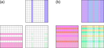
Figure 1: Algorithms for computing $\Theta$ matrices. (a) CPU-based implementation. A subset of bonds are selected from $\Gamma^{[k]},\Gamma^{[k+1]}$ that have the correct selected charge values $c^{[k-1]},c^{[k+1]}$. A subset of $\Theta$ is computed. (b) GPU-based implementation. All bonds are used and the entire $\Theta$ matrix is computed at once.

II.2 Hierarchical GPU implementation

If each thread computes one entry of $\Theta$, there is still much more data movement than computation per thread. In fact, memory bandwidth is a significant limiting factor in this case, and the computation gets starved by a lack of data. This issue is well addressed in optimized matrix multiplication kernels and tensor core operations, and we follow a similar approach to address this issue. For a pedagogical introduction to the hierarchical approach in the context of matrix multiplication, see the work by Kerr et. al. Kerr et al. (2017)

Consider an $M\times K$ matrix $A$ multiplying a $K\times N$ matrix $B$, both are stored in the global memory, the memory every thread can access. If each GPU thread computes one entry, the naive way is to make thread $i,j$ add $A_{i,k}B_{k,j}$ $K$ times through all $k$. In this algorithm, each thread requires $2K$ global reads, and the whole algorithm requires $2MNK$ global reads. However, the bandwidth for global memory access is low, limiting the performance.

Shared memory is the memory that threads in a thread block can access, and it is much faster than global memory. A block is a collection of (at most 2048) threads, and threads in a block can cooperate by sharing data through the shared memory. If a whole row/column of $A/B$ is saved in the shared memory by $M+N$ global reads, all the threads can accumulate $A_{i,k}B_{k,j}$ once by $2MN$ shared memory reads. If this is repeated $K$ times through all $k$, we would only need $K(M+N)$ global reads and $2MNK$ shared memory reads. In short, we can replace element-wise inner products with the accumulation of outer products to reduce the memory read requirement, and Fig. 2 illustrates the differences between the two approaches. In reality, since a thread block has a limited number of threads and shared memory, we cannot fit everything in a single block and must compute the entire output matrix by sub-blocks.

Figure 2: Matrix multiplication with (a) inner products and (b) outer products.

A similar approach of shifting the need for high shared memory reads to faster memory access can be achieved. We can break each block into a warp tile, and a warp into a thread tile. Each thread is responsible for multiple indices, a fragment of the matrix, instead of just one element. This allows data to be stored in registers, which are private to each thread and much faster than shared memory.

We adopt all aforementioned techniques in our GPU kernel for obtaining $\Theta(c^{k})$, with the added complexity of complex number support and $U$ matrix value look-up based on charges. Software pipelining in standard matrix multiplication kernels is also implemented to hide data movement latency.

II.3 Memory alignment in GPU implementation

The charge data-dependent access of $U$ poses difficulties in efficient GPU parallelization. Normally, parallel threads over which computational load is distributed read and write data to memory locations in an aligned manner. Alignment means consecutive threads read and write to consecutive memory addresses, which allows data to be sent in chunks rather than one address at a time. If we distribute the computation of each bond index of $\Theta$ over each thread, it will be completely unpredictable which address of $U$ the thread has to read since it depends on the charge of the bond, and aligned memory access is impossible.

To address this issue, we propose to sort the bonds according to their charges before GPU computation. This leads to aligned memory access as illustrated in Fig. 3 and significantly improves performance. Additionally, since thread-level tiling requires each thread to compute for multiple indices/bonds, each thread can potentially encounter multiple charge values even after sorting the bonds by charge. This rapidly increases the number of registers needed per thread, which is a limited resource. Therefore, we insert empty bonds to ensure that the charges only change in multiples of the fragment dimension, ensuring that only one value of the unitary matrix corresponding to a single charge $c$ and physical state $i$ value is stored per thread. This scheme is illustrated in Fig. 4.

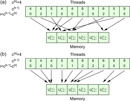
Figure 3: Memory access pattern (a) without sorting and (b) with sorting.

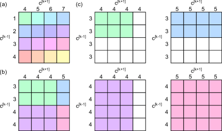
Figure 4: Illustration of insertion of empty bonds. (a) Worst case scenario of charge value changes within a single fragment without empty bond insertion. The thread has to store 16 values of the unitary. (b) Generic case of a fragment at a charge change boundary. Less than 16 values need to be stored, but this is not known a-priori and 16 values of the unitary still needs to be stored. (c) With empty bond insertion, each thread only needs one unitary value.

Additionally, bond indices are sorted such that $c_{\alpha_{k}}^{[k]}$ only increases as the bond index increases. For small $d$, this means that $c_{\alpha_{k}}^{[k]}$ is the same for many consecutive indices. This eliminates the need for threads to look up new $U$ elements, except at boundaries where $c_{\alpha_{k}}^{[k]}$ changes. This further reduces the need for memory access and reduces latency.

II.4 High-level parallelization

Besides the numerical parallelization of individual SVD and $\Theta$ matrix computations through the use of GPUs, additional parallelization is explicitly implemented on the algorithmic level. Further, for systems with large bond dimensions, storing the entire tensor network on a single-GPU or even a single node may become prohibitive. We distribute the storage of individual $\Gamma$ tensors to different nodes.

First, we parallelize independent two-site unitary updates. A host node identifies all parallel local unitary updates and keeps track of a list of available and busy nodes. Local unitary updates are allocated as soon as a node is available. During allocation, the compute process of the computational node requests the needed $\Gamma,\lambda,c$ tensors from the storage processes of the corresponding storage nodes. Similar communication takes place after the computation to update the stored tensors.

Second, for a single beam splitter MPO update, the overall $\Theta$ matrix is broken up into $\Theta(c^{[k]})$’s. We can compute different $\Theta(c^{[k]})$’s and perform SVD on them in parallel, then consolidate the results at the end. After the computation node receives the data needed, the data needed for each $\Theta(c^{[k]})$ is distributed to individual GPUs.

With the high-level parallelization discussed above and illustrated in Fig. 5, the algorithm can be easily scaled to supercomputers with multiple nodes and GPUs, especially when the system size is large. However, there are smaller systems that do not require multi-node parallelization, and we provide implementations with intermediary parallelism as well to avoid the communication overhead of the fully parallel algorithm. On the lowest level, only one GPU is considered, and no distributed memory or computation is used. On the second level, all memory is managed by a single node, and unitary updates are distributed to individual GPUs instead of nodes.

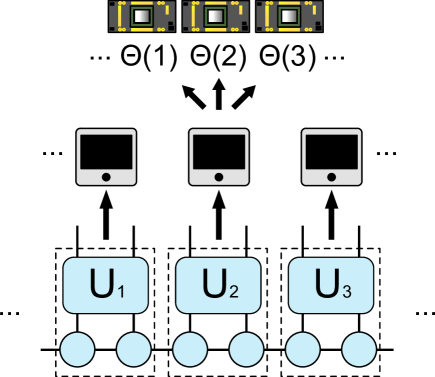
Figure 5: High-level parallelization. Independent unitary gate updates are distributed to different nodes. Within each unitary update, $\Theta(c^{[k]})$’s are computed and decomposed with SVD independently on different GPUs.

II.5 Run time reduction

We evaluate the performance of our GPU supercomputing algorithm against the CPU-only implementation at the Argonne Leadership Computing Facility (ALCF). All CPU simulations are performed with a single node of the Bebop system with a 2.10 GHz Intel Xeon E5-2695v4 32-core CPU, and GPU simulations are performed on the Polaris system. A single node of the Polaris system has 4 Nvidia A100 GPUs. Table I shows the simulation time in seconds of different implementations for a lossy boson sampling experiment with 12 modes, 10 input squeezed modes, bond dimension 1024 and 8192, photon loss rate 0.55, and local Hilbert space dimension 15. Increasing the bond dimension $\chi$ increases the simulation accuracy and time. Moreover, lossy boson sampling requires the density matrix instead of the state vector, and the generalized algorithm is described in detail in by Oh et. al. Oh et al. (2021) The consequence of the density matrix generalization is that each charge can take on $15^{2}=225$ values instead of only $15$, which means that the CPU-based algorithm needs to perform $225^{2}=50625$ iterations to fill the $\Theta$ matrix. On the other hand, our GPU algorithm computes all entries of $\Theta$ in parallel.

For the small $\chi$ experiment, we ar able to simulate using only CPUs in a reasonable amount of time for comparison. Encouragingly, the single-GPU algorithm achieves a dramatic 63-time speedup even with a single-GPU. We further test the unitary-level parallel algorithm on one node and observe a further two-fold speedup. Lastly, we use the fully parallel algorithm on 6 nodes, observing an additional 43% increase in the computational speed. We observe that the gain in computational speed by switching from less parallelized to highly parallelized implementation is less than the increase in computational resources. Higher-level parallelism incurs significant overhead, which indicates that there is still significant room for optimization.

Fortunately, this payoff in higher parallelism is more pronounced in the setting of larger system sizes. The CPU implementation failed to complete the simulation within the maximum allowed wall time of $72$ hours. This means that our single-GPU implementation achieves at least a 125-fold speed up. The computational time is further reduced two-fold when going from the single-GPU implementation to the unitary-level parallel algorithm on one node, similar to the small bond dimension case. However, changing to the fully parallelized algorithm with 6 nodes further reduces the time more than three-fold compared to a fractional reduction in the small bond dimension case. Overall, the fully parallel implementation on six nodes is on the order of a 1000 times faster than the 32-core CPU implementation.

	CPU	single-GPU	One node	Six nodes
$\chi=1024$	7966	126	60	42
$\chi=8192$	>259000	2066	1045	322

Table 1: Simulation time in seconds.

III Discussion

We have shown that our GPU supercomputer algorithm dramatically speeds up $U(1)$ symmetric tensor network calculations through GPU-level and software-level parallelism. Specifically, we demonstrated greater than 125-fold speed up compared to the 32-core CPU implementation with a single-GPU, and a total speed up on the order of 1000 times when more resources are used. We believe that this tool will be especially valuable to the quantum many-body physics community due to its computational efficiency. Further, the formalism of tensor networks beyond MPS with other types of symmetry has already been developed Singh et al. (2010), and adaptation of our approach to accelerating these computational tools might be possible with additional theoretical and engineering research. Lastly, with the advent of exascale supercomputing such as the Aurora supercomputer, and hardware platform independent programming models such as SYCL and oneAPI, a new era of accelerated supercomputing tensor network algorithms for quantum physics holds a tremendous amount of promise. Overall, our algorithm opens up the possibility of simulating large many-body quantum systems that are $U(1)$ symmetric, which include a wide range of interesting systems including the Bose Hubbard model, spin systems, boson sampling, and quantum walk.

Data availability

There is not data generated from this work.

Code availability

The code described in this work is available in the GitHub repository https://github.com/sss441803/BosonSampling.

References

- White (1992) Steven R. White, “Density matrix formulation for quantum renormalization groups,” Phys. Rev. Lett. 69, 2863–2866 (1992).
- Vidal et al. (2003) G. Vidal, J. I. Latorre, E. Rico, and A. Kitaev, “Entanglement in quantum critical phenomena,” Phys. Rev. Lett. 90, 227902 (2003).
- Verstraete and Cirac (2004) Frank Verstraete and J Ignacio Cirac, “Renormalization algorithms for quantum-many body systems in two and higher dimensions,” arXiv preprint cond-mat/0407066 (2004).
- Klümper et al. (1993) A. Klümper, A. Schadschneider, and J. Zittartz, “Matrix product ground states for one-dimensional spin-1 quantum antiferromagnets,” Europhysics Letters 24, 293 (1993).
- Orús and Vidal (2008) R. Orús and G. Vidal, “Infinite time-evolving block decimation algorithm beyond unitary evolution,” Phys. Rev. B 78, 155117 (2008).
- Vidal (2004) Guifré Vidal, “Efficient simulation of one-dimensional quantum many-body systems,” Phys. Rev. Lett. 93, 040502 (2004).
- Oh et al. (2021) Changhun Oh, Kyungjoo Noh, Bill Fefferman, and Liang Jiang, “Classical simulation of lossy boson sampling using matrix product operators,” Phys. Rev. A 104, 022407 (2021).
- Huang et al. (2019) H.-L. Huang, W.-S. Bao, and C. Guo, “Simulating the dynamics of single photons in boson sampling devices with matrix product states,” Phys. Rev. A 100, 032305 (2019).
- Liu et al. (2023) Minzhao Liu, Changhun Oh, Junyu Liu, Liang Jiang, and Yuri Alexeev, “Complexity of gaussian boson sampling with tensor networks,” arXiv preprint arXiv:2301.12814 (2023).
- Liu et al. (2022a) Minzhao Liu, Junyu Liu, Rui Liu, Henry Makhanov, Danylo Lykov, Anuj Apte, and Yuri Alexeev, “Embedding learning in hybrid quantum-classical neural networks,” in 2022 IEEE International Conference on Quantum Computing and Engineering (QCE) (2022) pp. 79–86.
- Liu et al. (2022b) Minzhao Liu, Ge Dong, Kyle Gerard Felker, Matthew Otten, Prasanna Balaprakash, William Tang, and Yuri Alexeev, “Exploration of quantum machine learning and ai accelerators for fusion science,” (2022b), 10.2172/1840522.
- Lykov et al. (2021) Danylo Lykov, Angela Chen, Huaxuan Chen, Kristopher Keipert, Zheng Zhang, Tom Gibbs, and Yuri Alexeev, “Performance evaluation and acceleration of the qtensor quantum circuit simulator on gpus,” in 2021 IEEE/ACM Second International Workshop on Quantum Computing Software (QCS) (2021) pp. 27–34.
- Wurtz and Lykov (2021) Jonathan Wurtz and Danylo Lykov, “Fixed-angle conjectures for the quantum approximate optimization algorithm on regular maxcut graphs,” Phys. Rev. A 104, 052419 (2021).
- Lykov et al. (2022) Danylo Lykov, Roman Schutski, Alexey Galda, Valeri Vinokur, and Yuri Alexeev, “Tensor network quantum simulator with step-dependent parallelization,” in 2022 IEEE International Conference on Quantum Computing and Engineering (QCE) (2022) pp. 582–593.
- Liu et al. (2022c) Minzhao Liu, Junyu Liu, Yuri Alexeev, and Liang Jiang, “Estimating the randomness of quantum circuit ensembles up to 50 qubits,” npj Quantum Inf 8 (2022c), 10.1038/s41534-022-00648-7.
- Singh et al. (2011) Sukhwinder Singh, Robert N. C. Pfeifer, and Guifre Vidal, “Tensor network states and algorithms in the presence of a global u(1) symmetry,” Phys. Rev. B 83, 115125 (2011).
- Aizenman et al. (2004) Michael Aizenman, Elliott H. Lieb, Robert Seiringer, Jan Philip Solovej, and Jakob Yngvason, “Bose-einstein quantum phase transition in an optical lattice model,” Phys. Rev. A 70, 023612 (2004).
- Alcaraz et al. (1989) F.C. Alcaraz, U. Grimm, and V. Rittenberg, “The xxz heisenberg chain, conformal invariance and the operator content of c < 1 systems,” Nuclear Physics B 316, 735–768 (1989).
- Aaronson and Arkhipov (2011) S. Aaronson and A. Arkhipov, “The computational complexity of linear optics,” in Proceedings of the forty-third annual ACM symposium on Theory of computing (2011) pp. 333–342.
- Kitagawa et al. (2010) Takuya Kitagawa, Mark S. Rudner, Erez Berg, and Eugene Demler, “Exploring topological phases with quantum walks,” Phys. Rev. A 82, 033429 (2010).
- Childs (2010) A.M. Childs, “On the relationship between continuous- and discrete-time quantum walk,” Commun. Math. Phys. 294, 581–603 (2010).
- Childs et al. (2013) Andrew M. Childs, David Gosset, and Zak Webb, “Universal computation by multiparticle quantum walk,” Science 339, 791–794 (2013).
- Cai et al. (2021) Xiaoming Cai, Hongting Yang, Hai-Long Shi, Chaohong Lee, Natan Andrei, and Xi-Wen Guan, “Multiparticle quantum walks and fisher information in one-dimensional lattices,” Phys. Rev. Lett. 127, 100406 (2021).
- Schreiber et al. (2012) Andreas Schreiber, Aurél Gábris, Peter P. Rohde, Kaisa Laiho, Martin Štefaňák, Václav Potoček, Craig Hamilton, Igor Jex, and Christine Silberhorn, “A 2d quantum walk simulation of two-particle dynamics,” Science 336, 55–58 (2012).
- Agrawal et al. (2022) Utkarsh Agrawal, Aidan Zabalo, Kun Chen, Justin H. Wilson, Andrew C. Potter, J. H. Pixley, Sarang Gopalakrishnan, and Romain Vasseur, “Entanglement and charge-sharpening transitions in u(1) symmetric monitored quantum circuits,” Phys. Rev. X 12, 041002 (2022).
- Spring et al. (2013) J. B. Spring, B. J. Metcalf, P. C. Humphreys, W. S. Kolthammer, X.-M. Jin, M. Barbieri, A. Datta, N. Thomas-Peter, N. K. Langford, D. Kundys, et al., “Boson sampling on a photonic chip,” Science 339, 798–801 (2013).
- Zhong et al. (2021) Han-Sen Zhong, Yu-Hao Deng, Jian Qin, Hui Wang, Ming-Cheng Chen, Li-Chao Peng, Yi-Han Luo, Dian Wu, Si-Qiu Gong, Hao Su, et al., “Phase-programmable gaussian boson sampling using stimulated squeezed light,” Phys. Rev. Lett. 127, 180502 (2021).
- Madsen et al. (2022) L. S. Madsen, F. Laudenbach, M. F. Askarani, F. Rortais, T. Vincent, J. F. F. Bulmer, F. M. Miatto, L. Neuhaus, L. G. Helt, M. J. Collins, et al., “Quantum computational advantage with a programmable photonic processor,” Nature 606, 75–81 (2022).
- Wolf et al. (2008) Michael M. Wolf, Frank Verstraete, Matthew B. Hastings, and J. Ignacio Cirac, “Area laws in quantum systems: Mutual information and correlations,” Phys. Rev. Lett. 100, 070502 (2008).
- Guo and Poletti (2019) C. Guo and D. Poletti, “Matrix product states with adaptive global symmetries,” Phys. Rev. B 100, 134304 (2019).
- Nguyen et al. (2022) Thien Nguyen, Dmitry Lyakh, Eugene Dumitrescu, David Clark, Jeff Larkin, and Alexander McCaskey, “Tensor network quantum virtual machine for simulating quantum circuits at exascale,” ACM Transactions on Quantum Computing 4 (2022), 10.1145/3547334.
- Lyakh et al. (2022) Dmitry I. Lyakh, Thien Nguyen, Daniel Claudino, Eugene Dumitrescu, and Alexander J. McCaskey, “Exatn: Scalable gpu-accelerated high-performance processing of general tensor networks at exascale,” Appl. Math. Stat. 8 (2022).
- Kerr et al. (2017) Andrew Kerr, Duane Merrill, Julien Demouth, and John Tran, “Cutlass: Fast linear algebra in cuda c++,” (2017).
- Singh et al. (2010) Sukhwinder Singh, Robert N. C. Pfeifer, and Guifré Vidal, “Tensor network decompositions in the presence of a global symmetry,” Phys. Rev. A 82, 050301 (2010).