Distributed Resilient Interval Observers for Bounded-Error LTI Systems Subject to False Data Injection Attacks

Abstract

This paper proposes a novel distributed interval-valued simultaneous state and input observer for linear time-invariant (LTI) systems that are subject to attacks or unknown inputs, injected both on their sensors and actuators. Each agent in the network leverages a singular value decomposition (SVD) based transformation to decompose its observations into two components, one of them unaffected by the attack signal, which helps to obtain local interval estimates of the state and unknown input and then uses intersection to compute the best interval estimate among neighboring nodes. We show that the computed intervals are guaranteed to contain the true state and input trajectories, and we provide conditions under which the observer is stable. Furthermore, we provide a method for designing stabilizing gains that minimize an upper bound on the worst-case steady-state observer error. We demonstrate our algorithm on an IEEE 14-bus power system.

I Introduction

The control of Cyber-Physical Systems (CPS) relies on the tight integration of various computational, communication, and sensor components that interact with each other and with the physical world in a complex way. Applications of CPS are broad and include, to name a few, industrial infrastructures [1], power grids [2], and intelligent transportation systems [3]. In such safety-critical systems, serious detriment can occur in case of malfunction or if jeopardized by malicious attackers [4]. One of the most serious types of attacks consists of false-data injection, by which counterfeit data signals are injected into the actuator signals and sensor measurements by strategic and/or malicious agents. Such attacks are not well-modeled by zero-mean, Gaussian white noises nor by signals with known bounds, given their strategic nature. On the other hand, most of the centralized approaches to state estimation are computationally expensive, especially for realistic high-dimensional CPS. Consequently, reliable distributed state and unknown input estimation algorithms are indispensable for the sake of resilient control, attack identification, and mitigation.

Motivated by this, several estimation algorithms have been proposed, in which a central entity seeks to estimate both the system state and the unknown disturbance (input). In the context where the noise signals are Gaussian and white, a large body of work proposed different designs for joint input and state estimation via e.g., minimum variance unbiased estimation [5], modified double-model adaptive estimation [6], or robust regularized least square approaches [7]. However, these approaches are not applicable in the context of attack-resilient bounded error worst-case estimation against false data injection attacks, where no information about the distribution of uncertainties is available. In such a setting, numerous approaches were proposed for deterministic systems [8], stochastic systems [9], and bounded-error systems [10, 11, 12]. These approaches typically yield point estimates, i.e, the most likely or best single estimate, as opposed to set-valued estimates.

Set-valued estimates have the advantage of providing hard accuracy bounds, which are important to guarantee safety [13, 14, 15, 16]. In addition, the use of fixed-order set-valued methods can help decrease the complexity of optimal observers [17], which grows with time. Hence, fixed-order centralized set-valued observers were presented for different classes of systems [13, 18, 19, 20, 21, 22, 23], that simultaneously find bounded sets of compatible states and unknown inputs. However, these algorithms do not scale well in a networked setting as the size of the network increases. This motivates the design of distributed input and state filters, which have typically focused on systems with stochastic disturbances [24, 25]. While these methods are more scalable and robust to communication failures than their centralized counterparts, they generally have comparatively worse estimation error. Moreover, they are not applicable in bounded-error settings where no information about the stochastic characteristics of noise/disturbance is available. With that in mind, in our previous work [26] we provided a distributed algorithm to synthesize interval observers for bounded-error LTI systems, without considering unknown input signals (attacks). In this work we aim to extend our design in [26] to address resiliency against false data injection attacks, i.e., to synthesize distributed interval observers in the bounded-error settings that are stable and correct in the presence of unknown input/attack signals.

Contributions. This work aims to bridge the gap between distributed resilient estimation algorithms and interval observer design approaches in bounded-error settings and subject to completely unknown and/or distribution-free inputs (attacks). In other words, leveraging the notion of “collective positive detectability over neighborhoods” (CPDN), we provide a distributed algorithm that simultaneously synthesizes tractable and computationally efficient interval-valued estimates for states and unknown inputs of bounded error LTI systems, whose sensors and actuators are subject to false data injection attacks. We provide conditions for the stability of our proposed observer, which is shown to minimize a computed upper bound for the observer error interval widths.

II Preliminaries

This section introduces basic notation, preliminary concepts, and graph-theoretic notions used throughout the paper.

Notation. Let ${\mathbb{N}}$, $\mathbb{Z}_{\geq 0}$, $\mathbb{R}_{\geq 0}$, denote the sets of natural, nonnegative integer and real numbers, respectively. Similarly, ⁿ and ^n×p denote the $n$-dimensional Euclidean space, and the set of $n\times p$ matrices, respectively. Given $A^{1},\dots,A^{N}\in^{n\times n}$, $\operatorname{diag}(A^{1},\dots,A^{N})\in^{nN\times nN}$ is the block-diagonal matrix with block-diagonal elements $A^{i},i\in\{1,\dots,N\}$. For $M\in^{n\times p}$, $M_{i}$ and $M_{ij}$ denote the $i^{\textup{th}}$ row and the $(i,j)^{\textup{th}}$ entry of $M$, respectively. Furthermore, we define $M^{+}\in^{n\times p}$, such that $M^{+}_{ij}\triangleq\max\{M_{ij},0\}$, $M^{-}\triangleq M^{+}-M$, and $|M|\triangleq M^{+}+M^{-}$. All inequalities $\leq$, $\geq$, as well as $\max$ and $\min$, are considered element-wise. Given $M\in^{n\times n}$, $\rho(M)$ is used to denote the spectral radius of $M$. A multi-dimensional interval is denoted as $\mathcal{I}\triangleq[\underline{s},\overline{s}]\subset^{n}$, and is the set of vectors $x\in^{n}$ such that $\underline{s}\leq x\leq\overline{s}$.

Proposition 1.

[27, Lemma 1] Let $A\in^{p\times n}$ and $\underline{x}\leq x\leq\overline{x}\in^{n}$. Then, $A^{+}\underline{x}-A^{-}\overline{x}\leq Ax\leq A^{+}\overline{x}-A^{-}\underline{x}$. As a corollary, if $A$ is non-negative, $A\underline{x}\leq Ax\leq A\overline{x}$.

Graph-theoretic Notions. A directed graph $\mathcal{G}=(\mathcal{V},\mathcal{E})$ is a set of nodes $\mathcal{V}\triangleq\{1,\dots,N\}$ and edges $\mathcal{E}\subseteq\mathcal{V}\times\mathcal{V}$. The neighbors of node $i$, denoted $\mathcal{N}_{i}$, is the set of all nodes $j$ for which $(j,i)\in\mathcal{E}$. We will assume that $i\in\mathcal{N}_{i}$.

III Problem Formulation

System Assumptions. Consider a multi-agent system (MAS) consisting of $N$ agents, which interact over a time-invariant communication graph $\mathcal{G}$ . The agents are able to obtain individual measurements of a target system as described by the following LTI dynamics:

$$\begin{array}[]{ll}\mathcal{P}:\begin{cases}x_{k+1}=Ax_{k}+Bw_{k}+Gd_{k},&\\ y^{i}_{k}=C^{i}x_{k}+D^{i}v^{i}_{k}+H^{i}d_{k},&i\in\mathcal{V},k\in\mathbb{Z}_{\geq 0},\end{cases}\end{array}$$ (2)

where $x_{k}\in^{n}$ is the continuous state of the target system, $d_{k}\in\mathbb{R}^{n_{p}}$ is a malicious disturbance and $w_{k}\in\mathcal{I}_{w}\triangleq[\underline{w},\overline{w}]\subset^{n_{w}}$ is bounded process noise. At time step $k$, every agent $i\in\mathcal{V}$ takes a measurement $y^{i}_{k}\in^{{m^{i}}}$, known only to itself, which is perturbed by $v^{i}_{k}\in\mathcal{I}_{v}^{i}\triangleq[\underline{v}^{i},\overline{v}^{i}]\subset^{n_{v}^{i}}$, a bounded sensor (measurement) noise signal. Finally, $A\in^{n\times n}$, $B\in^{n\times n_{w}}$, $G\in^{n\times n_{p}}$, $C^{i}\in^{m^{i}\times n}$, $D^{i}\in^{m^{i}\times n^{i}_{v}}$, and $H^{i}\in^{m^{i}\times n_{p}}$ are system matrices known to all agents, where $\operatorname{rank}(H^{i})=r^{i}$. Note that no restriction is made on $H^{i}$ to be either the zero matrix (no direct feedthrough), or to have full column rank when there is direct feedthrough. The agents’ goal is to simultaneously estimate the trajectories of (2) as well as the unknown input $d_{k}$ in a distributed manner, when states are initialized in an interval $\mathcal{I}_{x}\triangleq[\underline{x}_{0},\overline{x}_{0}]\subset^{n}$, with $\underline{x}_{0},\overline{x}_{0}$ known to all agents.

Unknown Input Signal Assumptions. We make no assumption about the unknown signal $d_{k}$, i.e., we require no prior knowledge such as its distribution, dynamics, or bounds.

Remark 1.

System (2) can be easily extended to cover the case where different attack signals $d^{s}_{k}\in\mathbb{R}^{n_{s}}$ and $d^{o}_{k}\in\mathbb{R}^{n_{o}}$ with the corresponding matrices $\hat{G}\in\mathbb{R}^{n\times n_{s}}$ and $\hat{H}^{i}\in\mathbb{R}^{{m^{i}}\times n_{o}}$ are injected into the actuators and sensors, respectively. In this case, courtesy of the fact that the unknown input signals can be completely arbitrary, by lumping them into a newly defined unknown input signal $d_{k}\triangleq[(d^{s}_{k})^{\top}(d^{o}_{k})^{\top}]^{\top}\in\mathbb{R}^{n_{p}},n_{p}\triangleq n_{o}+n_{s}$, as well as defining ${G}\triangleq\begin{bmatrix}\hat{G}&0_{n\times n_{o}}\end{bmatrix}$, ${H}^{i}\triangleq\begin{bmatrix}0_{{m^{i}}\times n_{s}}&\hat{H}^{i}\end{bmatrix}$, we can equivalently transform the considered system to a new representation, precisely in the form of (2).

Definition 1 (State and Input Framers).

For an agent $i\in\mathcal{V}$, the sequences $\{\overline{x}^{i}_{k},\underline{x}^{i}_{k}\}_{k\geq 0}\subseteq^{n}$ are called upper and lower local state framers for $\mathcal{P}$ if $\underline{x}^{i}_{k}\leq x_{k}\leq\overline{x}^{i}_{k}$ for all $k\geq 0$. Moreover, we define the local state framer errors as

$$\begin{array}[]{rl}\underline{e}^{i}_{k}&\triangleq x_{k}-\underline{x}^{i}_{k},\ \overline{e}^{i}_{k}\triangleq\overline{x}^{i}_{k}-x_{k},\ \forall k\geq 0.\end{array}$$ (4)

Finally, the collective state framer error is defined as

$$\begin{array}[]{rl}e_{k}&\triangleq\begin{bmatrix}(\underline{e}^{1}_{k})^{\top}&(\overline{e}^{1}_{k})^{\top}&\cdots&(\underline{e}^{N}_{k})^{\top}&(\overline{e}^{N}_{k})^{\top}\end{bmatrix}^{\top}\in^{2Nn}.\\ \end{array}$$ (6)

The local input framers $\{\underline{d}^{i}_{k},\overline{d}^{i}_{k}\}$, the local input framer errors $\{\underline{\delta}^{i}_{k},\overline{\delta}^{i}_{k}\}$, and the collective input framer error $\delta_{k}$ are defined similarly with respect to the unknown input $d_{k}$.

The problem of designing a distributed resilient state and input interval observer addressed here is cast as follows:

Problem 1.

Given a multi-agent system, design a distributed resilient interval observer for $\mathcal{P}$, i.e., an algorithm that computes uniformly bounded state and input framers for $\mathcal{P}$.

IV Proposed Distributed Interval Observer

In this section, we describe our novel resilient distributed interval observer design, its stability, and a tractable distributed procedure for computing stabilizing observer gains.

IV-A Distributed Input and State Framer and its Correctness

Before describing our proposed observer, we first transform the system into an equivalent representation which decouples the problem of estimating the state and the adversarial input. Inspired by the work in [13], we carry out a singular value decomposition (SVD) on the feedthrough matrix $H^{i}$, which decomposes the unknown input signal into two components $d^{i}_{1,k}$ and $d^{i}_{2,k}$. Consequently, we obtain two constituents for the measurement signal: $z^{i}_{1,k}$, which is affected by the unknown input through an invertible feedthrough matrix $S^{i}\in\mathbb{R}^{r^{i}\times r^{i}}$, and $z^{i}_{2,k}$, which is not compromised by the unknown input signal. Then, (2) can be represented as

$$x_{k+1} =Ax_{k}+Bw_{k}+G^{i}_{1}d^{i}_{1,k}+G^{i}_{2}d^{i}_{2,k},$$ (7a)

$$z^{i}_{1,k} =C_{1}^{i}x_{k}+D_{1}^{i}v^{i}_{k}+S^{i}d^{i}_{1,k},$$ (7b)

$$z^{i}_{2,k} =C_{2}^{i}x_{k}+D_{2}^{i}v^{i}_{k},$$ (7c)

$$d^{i}_{k} =V^{i}_{1}d_{1,k}+V^{i}_{2}d_{2,k}.$$ (7d)

To increase readability, the details of the transformation and how to compute $V^{i}_{1}$, $V^{i}_{2}$, $G^{i}_{1}$, $G^{i}_{2}$, $C^{i}_{1}$, $C^{i}_{2}$, $D^{i}_{1}$, and $D^{i}_{2}$ are provided in Appendix A. We further define $M^{i}_{1}\triangleq(S^{i})^{-1}$ and the concatenated noise vector $\eta^{i}_{k}\triangleq[v^{i\top}_{k-1}\ w^{\top}_{k-1}\ v^{i\top}_{k}]^{\top}$ with upper and lower bounds:

$$\underline{\eta}^{i}\triangleq[\underline{v}^{i\top}\ \underline{w}^{\top}\ \underline{v}^{i\top}]^{\top}\ \text{and}\ \overline{\eta}^{i}\triangleq[\overline{v}^{i\top}\ \overline{w}^{\top}\ \overline{v}^{i\top}]^{\top}.$$

To obtain input and state estimates, we require that each agent has access to adequate measurements which are not compromised by the unknown input. The following assumption ensures this. We refer the reader to [13, Lemma 1] for a discussion on the necessity of this type of requirement in centralized estimation algorithms subject to adversaries. In a nutshell, unless this type of observability conditions hold, an adversary can arbitrarily drive system components around in a fully stealthy manner.

Assumption 1.

$C^{i}_{2}G^{i}_{2}$ is full column rank for every $i\in\mathcal{V}$. Hence, there exists $M^{i}_{2}=(C^{i}_{2}G^{i}_{2})^{\dagger}$ such that $M^{i}_{2}C^{i}_{2}G^{i}_{2}=I$.

It is worth noting that $C^{i}_{2}$ and $G_{2}^{i}$ are both affine transformations of $C$ and $G$, respectively. Moreover, adequacy of measurements plays an important role when applying a singular value decomposition on the direct feedthrough matrix in the output equation (cf. Appendix A for more details). We are ready to propose our recursive distributed simultaneous state and unknown input observer.

IV-B Distributed Input and State Framer and its Correctness

To address Problem 1, we propose a four-step procedure, summarized as the Distributed Simultaneous Input & State Interval Observer (DSISO) in Algorithm 1. i) State Propagation and Measurement Update: Given $\underline{x}^{i}_{k}$, $\overline{x}^{i}_{k}$, $z^{i}_{1,k}$, $z^{i}_{2,k}$, and $z^{i}_{2,k+1}$, each agent $i\in\mathcal{V}$ performs a state propagation and a local measurement update step using to-be-designed observer gains $L^{i}$ and $\Gamma^{i}\in^{n\times{m^{i}}}$:

$$\begin{split}\underline{x}^{i,0}_{k+1}&=\mathtt{A}^{i+}\,\underline{x}_{k}^{i}-\mathtt{A}^{i-}\overline{x}_{k}^{i}+\mathtt{L}^{i+}\underline{\eta}^{i}-\mathtt{L}^{i-}\overline{\eta}^{i}+\Psi^{i}\xi^{i}_{k+1},\\ \overline{x}^{i0}_{k+1}&=\mathtt{A}^{i+}\overline{x}_{k}^{i}-\mathtt{A}^{i-}\underline{x}_{k}^{i}+\mathtt{L}^{i+}\overline{\eta}^{i}-\mathtt{L}^{i-}\underline{\eta}^{i}+\Psi^{i}\xi^{i}_{k+1},\end{split}$$ (8)

where $\mathtt{A}^{i}$, $\mathtt{L}^{i}$, and $\Psi^{i}$, which define the observer dynamics, depend linearly on $L^{i}$ and $\Gamma^{i}$ and are described in Appendix B, and $\xi^{i}_{k+1}\triangleq\begin{bmatrix}(z^{i}_{1,k})^{\top}&(z^{i}_{2,k})^{\top}&(z^{i}_{2,k+1})^{\top}\end{bmatrix}^{\top}.$ We also note that $\mathtt{A}^{i}$ has the form $\mathtt{A}^{i}\triangleq T^{i}\hat{A}^{i}-L^{i}C_{2}^{i}$, where $T_{i}=I-\Gamma^{i}C_{2}^{i}$, and $\hat{A}^{i}$ depends only on parameters of $\mathcal{P}.$

ii) State Framer Network Update: Each agent $i$ shares its local state framers with its neighbors in the network, updating them by taking the tightest interval from all neighbors via intersection,

$$\underline{x}^{i}_{k}=\max_{j\in\mathcal{N}_{i}}\underline{x}^{j,0}_{k},\quad\overline{x}^{i}_{k}=\min_{j\in\mathcal{N}_{i}}\overline{x}^{j,0}_{k}.$$ (9)

We consider only one iteration of this operation for simplicity; the extension to multiple iterations is straightforward.

iii) Input Estimation: Given the state framers (9), agent $i\in\mathcal{V}$ leverages the state dynamics and its measurement of the system to compute local input framers as follows:

$$\begin{array}[]{rl}\underline{d}^{i,0}_{k}&=\mathtt{A}^{i+}_{d}\,\underline{x}^{i}_{k}-\mathtt{A}_{d}^{i-}\overline{x}^{i}_{k}+\mathtt{F}^{i+}\underline{\eta}^{i}-\mathtt{F}^{i-}\overline{\eta}^{i}+\Phi^{i}\xi^{i}_{k+1},\\ \overline{d}^{i,0}_{k}&=\mathtt{A}_{d}^{i+}\overline{x}^{i}_{k}-\mathtt{A}_{d}^{i-}\underline{x}^{i}_{k}+\mathtt{F}^{i+}\overline{\eta}^{i}-\mathtt{F}^{i-}\underline{\eta}^{i}+\Phi^{i}\xi^{i}_{k+1}.\end{array}$$ (12)

where $\mathtt{A}_{d}^{i}$, $\mathtt{F}^{i}$, and $\Phi^{i}$ are described in Appendix B.

iv) Input Framer Network Update: Finally, each agent $i$ shares its local input framers with its neighbors in the network, again taking the intersection,

$$\begin{split}\underline{d}^{i}_{k}=\max_{j\in\mathcal{N}_{i}}\underline{d}^{j,0}_{k},\quad\overline{d}^{i}_{k}=\min_{j\in\mathcal{N}_{i}}\overline{d}^{j,0}_{k},\end{split}$$ (13)

Remark 2.

There are many existing centralized interval observer designs in the literature that could potentially be used for step i). However, most of these methods rely on similarity transformations [28] which depend on the observation matrices $C^{i}$. In a multi-agent setting, use of these methods necessitates transforming to and from the original coordinates whenever estimates are shared over the network. Each repeated transformation incurs the so-called “wrapping effect” as a result of Proposition 1, which worsens the estimation error and negates the benefit of exchanging information over the network. We avoid this with the choice of (8), which is computed directly in the original coordinates.

Algorithm 1 DSISO  at node $i$.

1:$\underline{x}^{i}_{0}$, $\overline{x}^{i}_{0}$,; Output: $\{\underline{x}^{i}_{k},\overline{x}^{i}_{k},\underline{d}^{i}_{k},\overline{d}^{i}_{k}\}_{k\geq 0}$;

2:Compute $L^{i}$ $\Gamma^{i}$, and $T^{i}$ by solving (18);

3:$k\leftarrow 1$

4:loop

5: $\triangleright$ State propagation and measurement update

6:     Compute $\underline{x}^{i,0}_{k}$ and $\overline{x}^{i,0}_{k}$ using (8);

7: $\triangleright$ State framer network update

8:     Send $\underline{x}^{i,0}_{k}$ and $\overline{x}^{i,0}_{k}$ to $\{j\ :\ i\in\mathcal{N}_{j}\}$;

9:     Receive $\underline{x}^{j,0}_{k}$ and $\overline{x}^{j,0}_{k}$ from $j\in\mathcal{N}_{i}$;

10:     $\displaystyle\underline{x}^{i}_{k}\leftarrow\,\max_{j\in\mathcal{N}_{i}}\underline{x}^{j,0}_{k};\quad\overline{x}^{i}_{k}\leftarrow\,\min_{j\in\mathcal{N}_{i}}\overline{x}^{j,0}_{k};$

11: $\triangleright$ Input framer estimation

12:     Compute $\underline{d}^{i,0}_{k}$ and $\overline{d}^{i,0}_{k}$ using (12);

13: $\triangleright$ Input framer network update

14:     Send $\underline{d}^{i,0}_{k}$ and $\overline{d}^{i,0}_{k}$ to $\{j\ :\ i\in\mathcal{N}_{j}\}$;

15:     Receive $\underline{d}^{j,0}_{k}$ and $\overline{d}^{j,0}_{k}$ from $j\in\mathcal{N}_{i}$;

16:     $\displaystyle\underline{d}^{i}_{k}\leftarrow\,\max_{j\in\mathcal{N}_{i}}\underline{d}^{j,0}_{k};\quad\overline{d}^{i}_{k}\leftarrow\,\min_{j\in\mathcal{N}_{i}}\overline{d}^{j,0}_{k};$

17:     $k\leftarrow k+1$;

18:end loop

19:return $\{\underline{x}^{i}_{k},\overline{x}^{i}_{k},\underline{d}^{i}_{k},\overline{d}^{i}_{k}\}_{k\geq 0}$

Lemma 1 (Distributed Framer Construction).

The DSISO algorithm outputs interval state and input framers for $\mathcal{P}$.

Proof.

See Appendix B. ∎

IV-C Distributed Stabilizing and Error Minimization

In this subsection, we investigate conditions on the observer gains $L^{i}$ and $\Gamma^{i}$, as well as the communication graph $\mathcal{G}$, that lead to an input-to-state stable (ISS) distributed observer, which equivalently results in a uniformly bounded observer error sequence given in (4)–(6), in the presence of bounded noise. To guarantee stability, we use the following assumption on the agents’ observation matrices and the structure of the network graph.

Assumption 2 (Collective Positive Detectability over Neighborhoods (CPDN) [26]).

For every state dimension $s\in\{1,\dots,n\}$ and every agent $i\in\mathcal{V}$, there is an agent $\ell(i,s)\in\mathcal{N}_{i}$ such that there exist gains $L^{\ell(i,s)}$, and $\Gamma^{\ell(i,s)}$ satisfying

$$\|(T^{\ell(i,s)}\hat{A}^{\ell(i,s)}-L^{\ell(i,s)}C_{2}^{\ell(i,s)})_{s}\|_{1}<1.$$

Intuitively, this assumption narrows the problem of stability to subgraphs. Within these subgraphs, we require that for each state dimension $s$, there is a node that, given estimates of all other state dimensions $\{1,\dots,s-1,s+1,\dots,n\}$, can compute an accurate estimate of dimension $s$. With this assumption in mind, we propose a two-step process to design the observer gains $L^{i}$ and $\Gamma^{i}$. First, each node executes a procedure (Algorithm 2) which verifies Assumption 2, returning false if it is not satisfied, or else computes some feasible stabilizing gains and the set of state dimensions which a node can contribute to estimating, i.e.,

$$\mathbb{J}^{i}\triangleq\{s\ :\ \exists T^{i},L^{i},\Gamma^{i}\text{ s.t. }\|(T^{i}\mathtt{A}^{i}-L^{i}C_{2}^{i})_{s}\|_{1}<1\}.$$

Then, given this information, each node solves the LP in (18), which simultaneously guarantees stability and minimizes an upper bound on the observer error. This design process improves on the one proposed in [26] in the absence of attacks, by first identifying “stabilizing” agents for each state dimension, then minimizing an upper bound on the error while enforcing the stability condition. In this way, the design includes a sense of noise/error attenuation. The following theorem formalizes our main results on how to tractably synthesize stabilizing and error minimizing observer gains in a distributed manner.

Theorem 1 (Distributed Input and State Interval Observer Design).

Suppose Assumptions 1 and 2 hold and $L^{i}_{*}$, $T^{i}_{*}$, and $\Gamma^{i}_{*}$ are solutions to the following convex program:

$$\begin{array}[]{rl}\min\limits_{Z^{i},L^{i},T^{i},\Gamma^{i}}&\quad\||\mathtt{L}^{i}|(\overline{\eta}^{i}-\underline{\eta}^{i})\|_{\infty}\\ \mathrm{s.t.}&\quad T^{i}=I-\Gamma^{i}C_{2}^{i},\\ &\quad\sum_{t=1}^{n}Z^{i}_{jt}<1,\ \forall j\in\mathbb{J}^{i},\\ &\quad-Z^{i}\leq T^{i}\hat{A}^{i}-L^{i}C_{2}^{i}\leq Z^{i},\\ \end{array}$$ (18)

where $\mathtt{L}^{i}$ is defined in (8) and $\mathbb{J}^{i}$ is calculated using Algorithm 2. Then, the DSISO algorithm, i.e., (8)–(13), with the corresponding observer gains $L^{i}_{*},T^{i}_{*},\Gamma^{i}_{*}$ constructs an ISS distributed input and state interval observer. Moreover, the steady state observer errors are guaranteed to be bounded:

$$\begin{array}[]{rl}\|e^{x}_{k}\|_{\infty}&\leq\frac{1}{1-\rho_{*}}\max_{i}\||\mathtt{L}^{i}|\Delta_{\eta}^{i}\|_{\infty},\\ \|\delta_{k}\|_{\infty}&\leq\frac{\rho(\mathcal{A}_{d})}{1-\rho_{*}}\max_{i}\||\mathtt{L}^{i}|\Delta_{\eta}^{i}\|_{\infty}+\max_{i}\||\mathtt{F}^{i}|\Delta_{\eta}^{i}\|_{\infty},\end{array}$$ (21)

where $\rho_{*}$, $\mathcal{A}_{d}$, and $\Delta_{\eta}^{i}$ are given in Lemma 2.

In order to prove our main results in Theorem 1, we need to first take two intermediate steps on i) providing closed form expressions for the observer errors and their upper bounds, and ii) ensuring the existence of stabilizing gains, stated via Lemmas 2 and 3, respectively. To begin, we note that equations (8)-(13) result in a switched linear system, with the following set of possible switching signals:

$$\mathcal{M}\triangleq\left\{M\in\{0,1\}^{2Nn\times 2Nn}\ :\begin{array}[]{c}M_{ij}=0,\forall j\notin\mathcal{N}_{i}\\ \sum_{k=1}^{2Nn}M_{ik}=1\end{array}\right\},$$

which encodes all possible permutations of the operation (9).

Lemma 2 (Error Bounds).

For all $\mathcal{B}\in\mathcal{M}$, the errors of the DSISO observer (8)–(13) are upper bounded as follows:

$$\begin{array}[]{rl}\|e^{x}_{k}\|_{\infty}&\leq\|e_{0}\|_{\infty}\rho_{*}^{k}+\frac{1-\rho_{*}^{k}}{1-\rho_{*}}\max_{i}\||\mathtt{L}^{i}|\Delta_{\eta}^{i}\|_{\infty},\\ \|\delta_{k}\|_{\infty}&\leq\rho(\mathcal{A}_{d})\|e_{k}\|_{\infty}+\max_{i}\||\mathtt{F}^{i}|\Delta_{\eta}^{i}\|_{\infty},\end{array}$$ (24)

where $\rho_{*}\triangleq\rho(\mathcal{B}\mathcal{A}_{x})$, $\mathcal{A}_{s}\triangleq\operatorname{diag}(\mathbb{A}^{1}_{s},\dots\mathbb{A}^{N}_{s})$, $\mathbb{A}^{i}_{s}\triangleq\begin{bmatrix}\mathtt{A}_{s}^{i+}&\mathtt{A}_{s}^{i-}\\ \mathtt{A}_{s}^{i-}&\mathtt{A}_{s}^{i+}\end{bmatrix},$ $\mathtt{A}^{i}_{x}\triangleq\mathtt{A}^{i}$, $s\in\{x,d\}$, and $\Delta_{\eta}^{i}\triangleq\overline{\eta}^{i}-\underline{\eta}^{i}.$

Proof.

Starting from (8)-(13) and following the lines of the proof of [26, Theorem 1], for any $\mathcal{B}\in\mathcal{M}$, the framer error s can be bounded by the positive linear comparison system

$$e_{k+1}\leq\mathcal{B}\mathcal{A}_{x}e_{k}+\mathcal{B}\gamma^{x}_{k},\quad\delta_{k}\leq\mathcal{A}_{d}e_{k}+\gamma^{d}_{k},$$ (25)

where $\forall s\in\{x,d\}:\gamma^{s}_{k}\triangleq[(\lambda^{1}_{s,k})^{\top}\dots\ (\lambda^{N}_{s,k})^{\top}]^{\top}$, $\lambda_{s,k}^{i}\triangleq\begin{bmatrix}((\Xi^{i}_{s})^{+}\underline{e}^{i}_{\eta,k}+(\Xi^{i}_{s})^{-}\overline{e}^{i}_{\eta,k})^{\top}&((\Xi^{i}_{s})^{-}\underline{e}^{i}_{\eta,k}+(\Xi^{i}_{s})^{+}\overline{e}^{i}_{\eta,k})^{\top}\end{bmatrix}^{\top}$, $\Xi^{i}_{x}\triangleq\mathtt{L}^{i},\Xi^{i}_{d}\triangleq\mathtt{F}^{i}$, $\underline{e}^{i}_{\eta,k}\triangleq\eta^{i}_{k}-\underline{\eta}^{i}_{k}$ and $\overline{e}^{i}_{\eta,k}\triangleq\overline{\eta}^{i}_{k}-\eta^{i}_{k}.$ Moreover, It follows from the solution of (25) that

$$e_{k}\leq(\mathcal{B}\mathcal{A}_{x})^{k-1}e_{0}+\sum_{s=1}^{k-1}(\mathcal{B}\mathcal{A}_{x})^{k-s}\gamma_{s-1}.$$ (26)

Further, $\|\gamma^{s}_{k}\|_{\infty}\leq\max_{i}|\Xi^{i}_{s}|(\overline{\eta}^{i}-\underline{\eta}^{i})$ by non-negativity of $(\Xi^{i}_{s})^{+}$, $(\Xi^{i}_{s})^{-}$, and $\overline{\eta}^{i}-\underline{\eta}^{i}$. The result follows from (25), (26), sub-multiplicativity of norms and the triangle inequality. ∎

Lemma 3.

If Assumption 2 holds, then there exist $L^{i}$ and $\Gamma^{i}$ such that, for some $\mathcal{B}_{*}\in\mathcal{M}$, $\mathcal{B}_{*}\mathcal{A}_{x}$ is Schur stable, i.e., $\rho(\mathcal{B}_{*}\mathcal{A}_{x})<1$. Consequently, the DSISO algorithm is ISS.

Proof.

It follows from combining [26, Theorems 1 $\&$ 2]. ∎

We are ready to provide a proof for Theorem 1 as follows.
Proof of Theorem 1. By Lemma 3, Assumption 2 implies the existence of gains that render the DSISO algorithm ISS. It remains to show that the solutions of (18) are stabilizing. First, notice that Algorithm 2 computes $\mathbb{J}^{i}$ by solving (29). The use of $\mathbb{J}^{i}$ in the constraints of (18) guarantees that the optimization problem is feasible. Furthermore, we can show that since Assumption 2 holds, there exists $\mathcal{B}_{*}$ such that $\rho(\mathcal{B}_{*}\mathcal{A}_{x})<1$, and therefore that the DSISO algorithm is ISS. We refer the reader to [26, Theorem 2] for the construction of $\mathcal{B}_{*}$. This in combination with Lemmas 2 and 3 ensures that the bounds in (24) converge to their steady state values in (21). ∎

Remark 3.

It is worth noting that by the following change of variables, the convex program in (1) can be easily and equivalently stated in the form of a linear program (LP):

$$\begin{array}[]{rll}\min\limits_{Z^{i},L^{i},T^{i},\Gamma^{i},\eta,\theta}&\quad\lambda\\ \mathrm{s.t.}&\quad\theta(\overline{\eta}^{i}-\underline{\eta}^{i})\leq\lambda\mathbf{1},\quad-\theta\leq\mathtt{L}^{i}\leq\theta,\\ &\quad T^{i}=I-\Gamma^{i}C_{2}^{i},\quad\sum_{t=1}^{n}Z^{i}_{jt}<1,\ \forall j\in\mathbb{J}^{i},\\ &\quad-Z^{i}\leq T^{i}\hat{A}^{i}-L^{i}C_{2}^{i}\leq Z^{i},\\ \end{array}$$

which can be considered as complementary to $\mathcal{H}_{\infty}$-optimal observer design, e.g., in [18, 19, 29].

Algorithm 2 DSISO initialization at node $i$.

1:$A$, $C^{i}$, $\mathcal{N}_{i}$; Output: $\mathbb{J}^{i}$

2:Compute $L_{*}^{i}$, $\Gamma_{*}^{i}$, and $Z_{*}^{i}$ by solving

$$\begin{array}[]{rl}\textstyle\min_{Z^{i},L^{i},\Gamma^{i}}&\quad\textstyle\sum_{s=1}^{n}\sum_{t=1}^{n}(Z^{i})_{st}\\ \mathrm{s.t.}&\ -Z^{i}\leq(I-\Gamma^{i}C_{2}^{i})\hat{A}^{i}-L^{i}C_{2}^{i}\leq Z^{i}.\end{array}$$ (29)

3:$\mathbb{J}^{i}\leftarrow\{s\ :\ \sum_{t=1}^{n}(Z_{*}^{i})_{st}<1\}$;

4:$\mathcal{Q}_{i}\leftarrow\{(I-\Gamma^{i}_{*}C_{2}^{i})\hat{A}^{i}-L_{*}^{i}C_{2}^{i}\}$;

5:Receive $\mathcal{Q}_{j}$ from $j\in\mathcal{N}_{i}$;

6:$\mathcal{Q}_{i}\leftarrow\bigcup_{j\in\mathcal{N}_{i}}Q_{j}$;

7:if $\forall s\in\{1,\dots,n\}$, $\exists P\in\mathcal{Q}_{i}$ s.t. $\|(P)_{s}\|_{1}<1$ then

8:     return false (i.e., Assumption 2 not satisfied)

9:else

10:     return $\mathbb{J}^{i}$

11:end if

V Simulation

In this section we demonstrate the DSISO algorithm on an IEEE 14-bus system [30]. We refer the reader to [8] for the derivation of the LTI representation of the system, which can be discretized and written in the form of (2). The $n=10$ dimensional state $x_{k}^{\top}=\begin{bmatrix}\delta_{k}^{\top}&\omega_{k}^{\top}\end{bmatrix}^{\top}$ represents the rotor angle and frequency of each of the 5 generators. Each bus in the test case corresponds to a node in the algorithm. The noise signals satisfy $\|w_{k}\|_{\infty}<5$ and $\|v^{i}_{k}\|<1\times 10^{-4}$ $\forall i\in\mathcal{V}$. Similarly to the example in [8], each node (bus) measures its own real power injection/consumption, the real power flow across all branches connected to the node, and for generating nodes, the rotor angle of the associated generator.

In this example, we assume that the generator at node 1 is insecure and potentially subject to attacks. Due to the reduction necessary to eliminate the algebraic constraints of the power system model [8], the disturbance appears directly in the measurements of all nodes, resulting in nonzero $H^{i}$ matrices. We compute the gains $L^{i}$ and $\Gamma^{i}$ by solving (18). Figures 1 and 2 show the input and state framers, respectively. It is clear that the algorithm is able to estimate the state $x_{1}$ despite the disturbance with only minor performance degradation. The switching due to (9), which depends on the noise, is also evident. The estimation performance for the other states is comparatively better, since they are only affected by (known) bounded noise. Furthermore, all agents are able to maintain an accurate estimate of the disturbance.

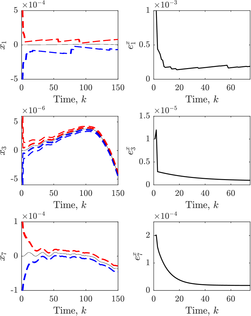
Figure 1: State upper (red) and lower (blue) framers from all agents and the true state value (black) for selected states $x_{1}$, $x_{3}$, and $x_{7}$ (left), as well as state error interval widths (right).

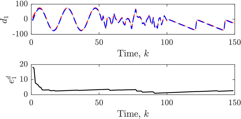
Figure 2: Unknown input framers and framer errors from all agents. Blue and red denote lower and upper framers, respectively, and black is the true signal.

VI Conclusion and Future Work

This paper introduced a novel distributed algorithm for interval estimates of states and unknown inputs for LTI systems with bounded noise, whose sensors and actuators are compromised by false data injection attacks. Without imposing any restrictive assumptions such as boundedness or stochasticity on the unknown input (attack) signals, we addressed the correctness of the proposed distributed observer, and moreover, analyzed the stability of the observer by considering the switched linear dynamics of the resulting error system. Finally, we provided a tractable method for computing stabilizing gains which aim to minimize the steady state input and state error of the observer. Hence, our approach can serve the purpose of resilient estimation in bounded-error networked cyber-physical systems. In the future, we consider extending our approach to nonlinear and hybrid systems, as well as including other type of adversarial effects such as switching and network attacks in our setting.

Appendix

VI-A Similarity Transformation

Let $r^{i}\triangleq\operatorname{rank}{(H^{i})}$. Using SVD, $H^{i}=\begin{bmatrix}U^{i}_{1}&U^{i}_{2}\end{bmatrix}\begin{bmatrix}S^{i}&0\\ 0&0\end{bmatrix}\begin{bmatrix}(V_{1}^{i})^{\top}\\ (V_{2}^{i})^{\top}\end{bmatrix}$, where $S^{i}\in\mathbb{R}^{r^{i}\times r^{i}}$ is a diagonal matrix of full rank, $U_{1}\in\mathbb{R}^{m^{i}\times r^{i}}$, $U_{2}\in\mathbb{R}^{m^{i}\times(m^{i}-r^{i})}$, $V_{1}\in\mathbb{R}^{n_{p}\times r^{i}}$ and $V_{2}\in\mathbb{R}^{n_{p}\times(n_{p}-r^{i})}$, while $U\triangleq\begin{bmatrix}U_{1}&U_{2}\end{bmatrix}$ and $V\triangleq\begin{bmatrix}V_{1}&V_{2}\end{bmatrix}$ are unitary matrices. Then, $d_{k}$ can be decoupled into two orthogonal components as: $d^{i}_{1,k}=(V_{1}^{i})^{\top}d_{k},d^{i}_{2,k}=(V_{2}^{i})^{\top}d_{k},d_{k}=V^{i}_{1}d^{i}_{1,k}+V^{i}_{2}d^{i}_{2,k},$ which transforms the system dynamics (2) to the representation in (7), where $G^{i}_{1}\triangleq GV^{i}_{1}$, $G^{i}_{2}\triangleq GV^{i}_{2}$, $H^{i}_{1}\triangleq H^{i}V^{i}_{1}=U^{i}_{1}S^{i},{C}^{i}_{1}\triangleq(U^{i}_{1})^{\top}{C}^{i},{C}^{i}_{2}\triangleq(U^{i}_{2})^{\top}{C}^{i},{D}^{i}_{1}\triangleq(U^{i}_{1})^{\top}{D}^{i}$, and ${D}^{i}_{2}\triangleq(U^{i}_{2})^{\top}{D}^{i}$.

VI-B Proof of Lemma 1

First, note that (7b) implies that

$$d^{i}_{1,k}=M^{i}_{1}(z^{i}_{1,k}-C_{1}^{i}x_{k}-D_{1}^{i}v^{i}_{k}).$$ (30)

This, in combination with (7c) and (7a) results in

$$M^{i}_{2}z^{i}_{2,k+1} =M^{i}_{2}(C_{2}^{i}x_{k+1}+D_{2}^{i}v^{i}_{k+1})$$

$$=M^{i}_{2}(C_{2}^{i}(Ax_{k}+Bw_{k}+G^{i}_{1}(M^{i}_{1}(z^{i}_{1,k}$$

$$\quad-C_{1}^{i}x_{k}-D_{1}^{i}v^{i}_{k})+G^{i}_{2}d^{i}_{2,k})+D_{2}^{i}v^{i}_{k+1}),$$

which given Assumption 1, returns

$$d^{i}_{2,k}=M^{i}_{2}(z^{i}_{k+1}-C^{i}_{2}(G^{i}_{1}M^{i}_{1}z^{i}_{1,k}+Q^{i}x_{k}))+E^{i}\eta_{k+1},$$ (31)

where $E^{i}=M_{2}^{i}\begin{bmatrix}C_{2}^{i}G_{1}^{i}M_{1}^{i}D_{1}^{i}&-C_{2}^{i}B&-D_{2}^{i}\end{bmatrix}$. By plugging $d_{1,k}^{i}$ and $d_{2,k}^{i}$ from (30) and (31) into (7a),

$$x_{k+1} =J^{i}Q^{i}x_{k}+\tilde{E}^{i}\eta^{i}_{k+1}+J^{i}G^{i}_{1}M^{i}_{1}z^{i}_{1,k}+G^{i}_{2}M^{i}_{2}C^{i}_{2}z^{i}_{2,k+1},$$

where $\tilde{E}=\begin{bmatrix}-J^{i}G_{1}^{i}M_{1}^{i}D_{1}^{i}&J^{i}B&-G_{2}^{i}M_{2}^{i}D_{2}^{i}\end{bmatrix}$. Combined with the fact that $T^{i}=I-\Gamma^{i}C^{i}_{2}$, this implies

$$x_{k+1}=T^{i}(J^{i}Q^{i}x_{k}+\tilde{E}^{i}\eta^{i}_{k+1}+\hat{z}^{i}_{k+1})+\Gamma^{i}C_{2}^{i}x_{k+1}.$$ (32)

Plugging in $C^{i}_{2}x_{k+1}=z^{i}_{2,k+1}-D^{i}_{2}v^{i}_{k+1}$ from (7c) and adding the zero term $L^{i}(z^{i}_{2,k}-C^{i}_{2}x_{k}-D^{i}_{2}v^{i}_{k})$ to the right hand side of (32), then collecting like terms, results in

$$x_{k+1}=\mathtt{A}^{i}x_{k}+\mathtt{L}^{i}\eta^{i}_{k+1}+\Psi^{i}\xi^{i}_{k+1},$$ (33)

By applying Proposition 1 to all the uncertain terms in the right hand side of (33): $\underline{x}^{i}_{k}\leq x_{k}\leq\overline{x}^{i}_{k}\Rightarrow\underline{x}^{i,0}_{k+1}\leq x_{k+1}\leq\overline{x}^{i,0}_{k+1}$, where $\underline{x}^{i,0}_{k+1},\overline{x}^{i,0}_{k+1}$ are given in (8). This means that individual framers/interval estimates are correct. When the framer condition is satisfied for all nodes, the intersection of all the individual estimates of neighboring nodes (cf. (9)) also results in correct interval framers, i.e.

$$\underline{x}^{i,0}_{k}\leq x_{k}\leq\overline{x}^{i,0}_{k},\;\forall i\in\mathcal{V}\implies\underline{x}^{i}_{k}\leq x_{k}\leq\overline{x}^{i}_{k},\;\forall i\in\mathcal{V}.$$

Furthermore, plugging $d^{i}_{1,k}$ and $d^{i}_{2,k}$ from (30) and (31) into (7d) and applying Proposition 1 returns the input framers in (12), where their intersection is still a framer (cf. (13)) by the same reasoning as for the state framers. Since the initial state framers are known to all $i$, by induction (8)-(13) constructs a correct distributed interval state and input framer for (2).

References

• [1] B. Cheng, J. Zhang, G.P. Hancke, S. Karnouskos, and A.W. Colombo. Industrial cyber-physical systems: Realizing cloud-based big data infrastructures. IEEE Industrial Electronics Magazine, 12(1):25–35, 2018.
• [2] J. Zhao, A. Gomez-Exposito, M. Netto, L. Mili, A. Abur, V. Terzija, I. Kamwa, B. Pal, A.K. Singh, J. Qi, Z. Huang, and A.P. Meliopoulos. Power system dynamic state estimation: Motivations, definitions, methodologies and future work. IEEE Transactions on Power Systems, 34:3188–3198, 07 2019.
• [3] Y. Sun and H. Song. Secure and trustworthy transportation cyber-physical systems. Springer, 2017.
• [4] K. Zetter. Inside the cunning, unprecedented hack of Ukraine’s power grid. Wired Magazine, 2016.
• [5] S. Z. Yong, M. Zhu, and E. Frazzoli. A unified filter for simultaneous input and state estimation of linear discrete-time stochastic systems. Automatica, 63:321–329, 2016.
• [6] P. Lu, E-J. Van Kampen, C.C. De Visser, and Q. Chu. Framework for state and unknown input estimation of linear time-varying systems. Automatica, 73:145–154, 2016.
• [7] M. Abolhasani and M. Rahmani. Robust deterministic least-squares filtering for uncertain time-varying nonlinear systems with unknown inputs. Systems & Control Letters, 122:1–11, 2018.
• [8] F. Pasqualetti, F. Dörfler, and F. Bullo. Attack detection and identification in cyber-physical systems. IEEE Transactions on Automatic Control, 58(11):2715–2729, November 2013.
• [9] H. Kim, P. Guo, M. Zhu, and P. Liu. Attack-resilient estimation of switched nonlinear cyber-physical systems. In American Control Conference (ACC), pages 4328–4333. IEEE, 2017.
• [10] Y. Nakahira and Y. Mo. Dynamic state estimation in the presence of compromised sensory data. In IEEE Conference on Decision and Control (CDC), pages 5808–5813, 2015.
• [11] M. Pajic, P. Tabuada, I. Lee, and G.J. Pappas. Attack-resilient state estimation in the presence of noise. In IEEE Conference on Decision and Control (CDC), pages 5827–5832, 2015.
• [12] S. Z. Yong, M.Q. Foo, and E. Frazzoli. Robust and resilient estimation for cyber-physical systems under adversarial attacks. In American Control Conference (ACC), pages 308–315. IEEE, 2016.
• [13] S. Z. Yong. Simultaneous input and state set-valued observers with applications to attack-resilient estimation. In American Control Conference (ACC), pages 5167–5174. IEEE, 2018.
• [14] F. Blanchini and M. Sznaier. A convex optimization approach to synthesizing bounded complexity $\ell^{\infty}$ filters. IEEE Transactions on Automatic Control, 57(1):216–221, 2012.
• [15] M. Khajenejad, F. Shoaib, and S.Z. Yong. Guaranteed state estimation via indirect polytopic set computation for nonlinear discrete-time systems. In 2021 60th IEEE Conference on Decision and Control (CDC), pages 6167–6174. IEEE, 2021.
• [16] M. Khajenejad, F. Shoaib, and S.Z. Yong. Guaranteed state estimation via direct polytopic set computation for nonlinear discrete-time systems. IEEE Control Systems Letters, 6:2060–2065, 2022.
• [17] M. Milanese and A. Vicino. Optimal estimation theory for dynamic systems with set membership uncertainty: An overview. Automatica, 27(6):997–1009, 1991.
• [18] M. Khajenejad and S. Z. Yong. Simultaneous input and state set-valued $\mathcal{H}_{\infty}$-observers for linear parameter-varying systems. In American Control Conference (ACC), pages 4521–4526, 2019.
• [19] M. Khajenejad and S.Z Yong. Simultaneous mode, input and state set-valued observers with applications to resilient estimation against sparse attacks. In 2019 IEEE 58th Conference on Decision and Control (CDC), pages 1544–1550, 2019.
• [20] M. Khajenejad, Z. Jin, and S.Z. Yong. Interval observers for simultaneous state and model estimation of partially known nonlinear systems. In American Control Conference (ACC), pages 2848–2854, 2021.
• [21] N. Ellero, D. Gucik-Derigny, and D. Henry. An unknown input interval observer for LPV systems under ${L}_{2}$-gain and ${L}_{\infty}$-gain criteria. Automatica, 103:294–301, 2019.
• [22] M. Khajenejad and S.Z. Yong. $\mathcal{H}_{\infty}$-optimal interval observer synthesis for uncertain nonlinear dynamical systems via mixed-monotone decompositions. IEEE Control Systems Letters, 6:3008–3013, 2022.
• [23] T. Pati, M. Khajenejad, S.P. Daddala, and S.Z. Yong. ${L}_{1}$-robust interval observer design for uncertain nonlinear dynamical systems. IEEE Control Systems Letters, 6:3475–3480, 2022.
• [24] Y. Lu, L. Zhang, and X. Mao. Distributed information consensus filters for simultaneous input and state estimation. Circuits, Systems, and Signal Processing, 32(2):877–888, Apr 2013.
• [25] A. E. Ashari, A. Y. Kibangou, and F. Garin. Distributed input and state estimation for linear discrete-time systems. In 2012 IEEE 51st IEEE Conference on Decision and Control, pages 782–787, 2012.
• [26] M. Khajenejad, S. Brown, and S. Martínez. Distributed interval observers for bounded-error LTI systems. In American Control Conference (ACC), accepted, https://arxiv.org/pdf/2209.01279.pdf, 2023.
• [27] D. Efimov, T. Raïssi, S. Chebotarev, and A. Zolghadri. Interval state observer for nonlinear time varying systems. Automatica, 49(1):200–205, 2013.
• [28] F. Mazenc, T.N. Dinh, and S.I. Niculescu. Interval observers for discrete-time systems. International journal of robust and nonlinear control, 24(17):2867–2890, 2014.
• [29] M. Khajenejad and S.Z. Yong. Resilient state estimation and attack mitigation in cyber-physical systems. In Security and Resilience in Cyber-Physical Systems, pages 149–185. Springer, 2022.
• [30] IEEE 14 Bus Test Case. URL: http://labs.ece.uw.edu/pstca/pf14/pg_tca14bus.htm.