Closed vortex state in 3D mesoscopic superconducting films under an applied transport current

Abstract

By using the full 3D generalized time dependent Ginzbug-Landau equation we study a long superconducting film of finite width and thickness under an applied transport current. We show that, for sufficiently large thickness, the vortices and the antivortices become curved before they annihilate each other. As they approach the center of the sample, their ends combine, producing a single closed vortex. We also determine the critical values of the thickness for which the closed vortex sets in for different values of the Ginzburg-Ladau parameter. Finally, we propose a model of how to detect a closed vortex experimentally.

I Introduction

One of the most outstanding physical phenomena in condensed matter theory is the flux quantization in the Shubnikov phase of superconducting materials. In bulk type-II superconductors, above a certain critical value of applied field, magnetic flux penetrates the sample in the form of flux quanta (in units of $\Phi_{0}=hc/2e$), the so called magnetic vortices. Superconducting vortices are very important due to their possible use in many applications, ranging from single photon detectors to quantum information. Moreover, the knowledge of how vortices behave under various circumstances is fundamental to the optimization of many electronic devices, since the vortex motion causes energy dissipation in a superconductor.

In the core of a superconducting vortex, the order parameter that describes the superconducting state vanishes and its phase changes by a multiple of $2\pi$ when circulated around a closed loop that encloses the core. As the vortex line tends to align with the direction of the magnetic field, in the presence of an external field applied perpendicularly to a superconducting film, the core of the vortex is rigorously a straight line with the currents flowing around it. This is the so called Abrikosov vortex, first described in his outstanding work [1].

However, the circularly shaped magnetic self-field induced by a current produces an Abrikosov vortex with a ringlike shape, which is usually called a closed vortex. This new type of solution was first found by Kozlov and Samokhvalov [2] through the solution of the London equation and was extensively studied further in Refs. [3, 4, 5, 6, 7, 8, 9, 10, 11, 12]. In these works, the existence, dynamics and even stability of such closed vortices in the presence of inhomogeneities were studied for unbounded superconductors or superconducting samples in the shape of a cylinder. In the latter case, due to matching symmetry between the field lines produced by the current and the cylinder geometry, the vortex penetrates the superconductor already in the form of a closed ring. Recently, these closed vortices were also shown to exist in a more complex geometry, such as a superconducting torus. [13]

In different scenarios, the formation of closed vortices was also recently studied, for example, in Josephson junctions [14] submitted to an external current, where it was shown that Josephson vortices can also be found in the form of closed vortex loops and a procedure to their experimental observation was introduced. Due to short life time of the Abrikosov closed vortices, their experimental detection is a difficult task and has not been accomplished so far. Recently, by using the microscopic theory of superconductivity Fyhn and Linder [15] proposed an experimental setup to the observation of such objects based on STM measurements. One of the most important results of the present work is to provide a new procedure to the detection of closed vortex loops, which is based on the measurement of the magnetic field profile produced by them. It is worth mentioning that, in practice, half-closed vortices have been demonstrated in RF cavities. [16]

In the present work, we study the physics of the closed vortices in a different setup. Namely, we investigate how a closed vortex emerges and gets annihilated in a superconducting slab under the presence of a transport current. Unlike previous works on the subject, the geometry of our superconductor does not favor the formation of a closed vortex. Here, this object is created solely by the inhomogeneous action of the applied current in different parts of the flux line. The study of the vortex dynamics is of fundamental importance to the understanding of the resistive state of current driven superconductors. Here, we show that, for appropriate thickness of the slab and Ginzburg-Landau parameter $\kappa$, a closed vortex forms in the process of annihilation of a vortex-antivortex (v-av) pairs induced in the sample by the current self-field. As we show, the lines corresponding to the vortex and the antivortex combine and form a closed loop when the pair is annihilating. After this combination, the loop takes the form of a quasi-ellipse, with the aspect ratio gradually decreasing until the collapse of the loop. By increasing the thickness of the film, the loop tends to a circle.

The outline of this work is as follows. In Sec. II we present our model and the formalism we used in order to solve the generalized Ginzburg-Landau equations [17, 18]. In Sec. III we present and discuss the results obtained in our simulations. Finally, we present our concluding remarks in Sec. IV.

II Theoretical model

In this work, we rely on the generalized time dependent Ginzburg-Landau (GTDGL) equation which is more suitable to describe the resitive state of dirty superconductors in the non-equilibrium state [17, 18]. In dimensionless units this equation is given by

$$\frac{u}{\sqrt{1+\gamma^{2}|\psi|^{2}}}\left[\frac{\partial}{\partial t}+\frac{1}{2}\gamma^{2}\frac{\partial|\psi|^{2}}{\partial t}\right]\psi=$$

$$=\left(\mbox{\boldmath$\nabla$}-i\textbf{A}\right)^{2}\psi+\psi(1-|\psi|^{2}),$$ (1)

coupled with Ampère’s law

$$\Sigma\frac{\partial\textbf{A}}{\partial t}=\textbf{J}_{s}-\kappa^{2}\mbox{\boldmath$\nabla$}\times\textbf{h},$$ (2)

where

$$\textbf{J}_{s}={\rm Im}\left[\bar{\psi}{(\mbox{\boldmath$\nabla$}-i\textbf{A})}\psi\right]$$ (3)

is the superconducting current density.

Here, the temperature is in units of the critical temperature $T_{c}$; the order parameter $\psi$ is in units of $\psi_{\infty}(T)=\sqrt{\alpha(T)/\beta}$, where $\alpha$ and $\beta$ are two phenomenological constants; the distances are measured in units of the coherence length $\xi(T)$; the vector potential A is in units of $\xi H_{c2}(T)$, where $H_{c2}$ is the upper critical field; the local magnetic field $\textbf{h}=\mbox{\boldmath$\nabla$}\times\textbf{A}$ is units of $H_{c2}(T)$; time is in units of the Ginzburg-Landau characteristic time $\tau_{GL}=\pi\hbar/8k_{B}Tu$; the material dependent parameter $\gamma=2\tau_{E}\Delta_{0}/\hbar$, where $\tau_{E}$ is the inelastic electron-collision time, and $\Delta_{0}$ is the gap in the Meissner state; the constant $\Sigma=4\pi\sigma D/c^{2}\xi^{2}(T)$, where $D$ is the diffusion coefficient and $\sigma$ is the normal state electrical conductivity; $\kappa=\lambda(T)/\xi(T)$ is the Ginzburg-Landau parameter, where $\lambda(T)$ is the London penetration depth; and finally, the constant $u$ is equal to 5.79, which is derived from first principles [17].

The original GTDGL equations take into account the scalar electrical potential $\varphi$. Since they are invariant under the following gauge transformations

$$\psi^{\prime} = e^{-i\chi}\psi,$$

$$\textbf{A}^{\prime} = \textbf{A}-\mbox{\boldmath$\nabla$}\chi,$$

$$\varphi^{\prime} = \varphi+\frac{\partial\chi}{\partial t},$$ (4)

where $\chi$ is an arbitrary scalar function therefore, we conveniently use the Weyl gauge [19] in which the scalar potential is constant and equal to zero.

In the present work, we consider an infinite superconducting film carrying a transport current as sketched in Fig. 1. The applied transport current is introduced as follows. The superconductor is in the presence of an applied electric field which is sustained by a DC transport current density which flows along the $x$ axis, $\textbf{J}_{a}=J_{a}\hat{\textbf{x}}$ . In the normal state, the vector potential has only the $x$ component. Thus, we separate the vector potential and the local magnetic field into two contributions, one coming from the normal state, and another one due to the diamagnetic nature of the superconductor that tends to cancel out the field induced by the applied current inside the sample. In other words, in Eqs.1-3 we substitute:

A $$= \textbf{A}_{0}+\textbf{A}_{1},$$ (5)

h $$= \textbf{h}_{0}+\textbf{h}_{1},$$ (6)

where A₀ and h₀ satisfy the following equations:

$$\kappa^{2}\mbox{\boldmath$\nabla$}\times\textbf{h}_{0}=J_{a}\hat{\textbf{x}},\;\;\;\kappa^{2}\nabla^{2}A_{0x}=-J_{a}\,.$$ (7)

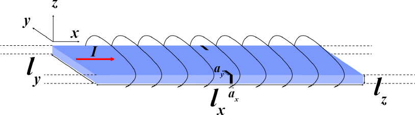
Figure 1: Schematic view of the system under consideration: an infinitely long superconducting sample of width $l_{y}$ and thickness $l_{z}$; only one unit cell of length $l_{x}$ is shown. The transport current is applied in the $x$ direction. The encircling lines illustrate the line fields of the self-field produced by the current. Two defects are introduced at the border of the sample (black spots), in order to facilitate nucleation of v-av pairs.

The analytical solutions of equations (7) are given in the Supplementary Material of Ref. [20].

Here, we solve the full 3D GTDGL equations numerically for an infinite superconducting film of finite width and thickness (see Fig. 1). The infinitely long film is divided into unit cells of dimensions $(l_{x},l_{y},l_{z})$. We take into account the demagnetization effects. Therefore, for numerical purposes, we must consider the unit cell inside a simulation box (not shown in Fig. 1) of dimensions $(l_{x},L_{y},L_{z})$, where $(L_{y},L_{z})$ are sufficiently larger than $(l_{y},l_{z})$ so that the demagnetizing field $\textbf{h}_{1}$ vanishes far away from the superconducting surfaces (for more details see Ref. [21]). In addition, the normal components of the superconducting current density of must be zero on the superconductor-vacuum interfaces. Then, the following boundary conditions must be fulfilled:

$$\hat{\textbf{n}}\cdot(\mbox{\boldmath$\nabla$}-i\textbf{A}_{0}-i\textbf{A}_{1})\psi = 0,\;\;\;\textrm{in}\;\partial\Omega_{sc},$$ (8)

$$\mbox{\boldmath$\nabla$}\times\textbf{A}_{1} = 0,\;\;\;\textrm{in}\;\partial\Omega,$$ (9)

where $\partial\Omega_{sc}$ and $\partial\Omega$ stand for superconducting and simulation box surfaces, respectively.

The two black spots in Fig. 1 represent two defects on the border of the sample. They are introduced as an artifact to create an inhomogeneity in the current, that induces the vortices and antivortices in the opposite sides of the sample.

III Results and discussion

III.1 Parameters and Methodology

The above equations are discretized by using the standard link-variable method as described in Ref. [22]. This algorithm is then implemented in Fortran 90 programming language and run in a GPU (Graphics Processing Unit) accelerated forward-time-central-space scheme.

In the simulations, we have fixed some parameters and varied others as follows. The length and width of the unit cell are fixed as $l_{x}=12\xi$ and $l_{y}=8\xi$. The thickness of the sample varied from $l_{z}=1\xi$ to $l_{z}=3.6\xi$ in increments of $0.2\xi$. We use $\kappa=1/\sqrt{2},1,\sqrt{3}$ for each set of values of $l_{z}$. The grid space used is $\Delta x=\Delta y=0.2\xi$ and $\Delta z=0.1\xi$. The size of the simulation box was chosen sufficiently large in order to satisfy boundary conditions (9); we use $l_{y}=16\xi$ and $l_{z}=12\xi$. The dimensions of the defects are $a_{x}=a_{y}=0.2\xi$. The range $10\leq\gamma\leq 20$ is suitable for most metals like Nb [17, 18, 23]; we used $\gamma=10$.

Let us explain how we calculate the IV (current-voltage) and IR (current-resistance) characteristics, which are the measurable quantities in the resistive state. In the Weyl gauge, the electrical field is given by $\textbf{E}=-\partial\textbf{A}/\partial t$, so, assuming that the voltage is measured between electrodes at $z=0$ that cover the width of the film, the voltage across a unit cell is:

$$U(t) = -\frac{1}{n_{y}-1}\sum_{j=2}^{n_{y}}\int_{-l_{x}/2}^{l_{x}/2}\,E_{x}(x,y_{j},0)dx$$ (10)

$$= \frac{1}{n_{y}-1}\sum_{j=2}^{n_{y}}\int_{-l_{x}/2}^{l_{x}/2}\frac{\partial A_{x}(x,y_{j},0)}{\partial t}dx,$$

where $n_{y}=l_{y}/\Delta y$, and $y_{j}=(j-n_{y}/2-1)\Delta y$ for are the $y$ coordinates of the mesh points. The voltage is then calculated as a time average of $U(t)$. We have:

$$V=\frac{1}{\cal T}\,\int_{0}^{\cal T}\,U(t)\,dt,$$ (11)

where ${\cal T}$ is the time corresponding to an appropriate number of oscillations of $U(t)$.

The applied current density was adiabatically increased in steps of $\Delta J_{a}=0.01J_{GL}$ from the Meissner state until the superconductivity was fully destroyed. In the resistive state, we moved from value of $J_{a}$ to $J_{a}+\Delta J_{a}$ only after the voltage $U(t)$ became periodic, which is the same periodicity with which the v-av pairs are formed and annihilated. When multiple nucleations of v-av (vortex-antivortex) pairs are present, the voltage looses its periodicity, and therefore we change the value of $J_{a}$ only after 220 oscillations of $U(t)$ in order to obtain a more accurate value of the time average voltage.

The results of all simulations are compiled in the following Subsections.

III.2 Field Profile, Closed Vortex, and Current Distribution

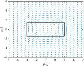
Figure 2: The magnetic field profile in the vertical plane $x=0$ (parallel to the $yz$ plane): for better visualization purposes, the arrows are not in real size; the rectangle inside is a cross section of the superconductor; this picture is for $\kappa=1$, $l_{y}=8\xi$, $l_{z}=3\xi$; the value of the current density is $J_{a}=0.26J_{GL}$ just before the critical current density $J_{c1}=0.27J_{GL}$. The vortex (antivortex) nucleates on the right-hand side (left hand-side) of the figure.

In Fig. 2 we illustrate the vector field profile at $x=0$ plane (in the middle of the unit cell, where the defects are located). The local field has symmetry as if the current density was uniform. Due to the geometric symmetry and the demagnetization effect, the local magnetic field is larger near the surface of the superconductor, and decreases deep inside. As can also be observed, the field is larger on the lateral sides of the sample. In this figure, we show the vector field for a value of the current density just before the first critical current $J_{c1}=0.27J_{GL}$. Therefore, once the resistive state sets in, it is on the lateral sides that the vortex and the antivortex sprout, move to the center, and finally annihilate each other at the center of the sample. Then, a periodic collapsing of v-av pairs is established.

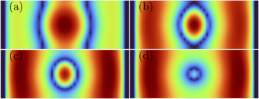
Figure 3: Color maps of the superconducting Cooper-pair density, $|\psi|$, for $\kappa=1$, $l_{z}=3\xi$, and $J_{a}=0.27J_{GL}$ throughout the plane $x=0$: (a) a v-av pair of curved vortices; on the left hand-side (right hand side) is the antivortex (vortex); (b) a combination of a vortex and an antivortex producing a closed vortex; (c) a closed vortex diminishing its radius; (d) a closed vortex shrinking down at the center. The dark strips on both sides are due to the defects. These pictures correspond to the same region highlighted in Fig. 2.

Next, we discuss the morphology of a closed vortex in the resistive state. The first works about closed vortices were conducted on long current-carrying superconducting cylinders, so that the vortex follows the geometry of the sample since from the surface until it collapses at the center [4, 7]. In the present scenario, we deal with a film of rectangular cross section. Thus, before the closed vortex is formed, two curved vortices (a vortex and an antivortex) nucleate in opposite sides of the sample (see panel (a) of Fig. 3) and move toward the center. Then, as they encounter each other, their ends join together forming a closed vortex (panel (b)). Once this ringlike vortex is formed, its radius starts decreasing (panel (c)) until it collapses at the center. After the transition from the Meissner state to the resistive one, the process is repeated periodically until superconductivity is suppressed throughout the sample.

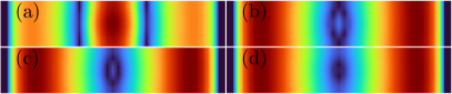
Figure 4: The same as in Fig.3 for $l_{z}=1.6\xi$ and $J_{a}=0.30J_{GL}$.

It is conceivable that the closed vortex can exist for any thickness of the film, but for small values of $l_{z}$ is very elongated when the ends of the v-av pair meet. In our simulations, we do not have sufficient resolution to detect a closed vortex for any $l_{z}$. Indeed, in Fig. 4 we show four panels of the color maps of the superconducting Cooper-pair density for $l_{z}=1.6\xi$. As we can see, the shape of the closed vortex is much more elongated than for the previous case $l_{z}=3\xi$ of Fig. 3. For $\kappa=1$, and thickness below $l_{z}=1.6\xi$, we do not observe any closed vortex; the v-av pair remains straight lines, since the nucleation of the vortex and the antivortex on the surfaces, until the pair is annihilated at the center of the sample. The formation of a closed vortex depends on the sample thickness because the current and the magnetic field concentrate near the surface of the superconductor, on a scale of the order of the London penetration depth. Therefore, for thicker samples, the ends of a vortex line are subjected to stronger Lorentz force and to a stronger horizontal magnetic field that facilitate the formation of a closed vortex.

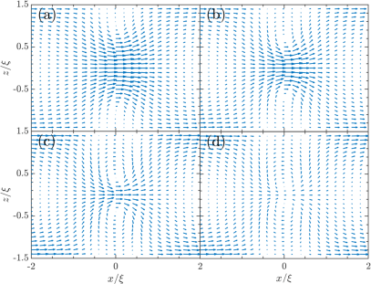
Figure 5: The panels show four cuts of the current distribution of the closed vortex throughout the vertical plane $y=0$. The radius of the closed vortex diminishes from (a) to (d).

Let us now discuss the current distribution of a closed vortex. When both curved vortex and antivortex touch their ends on the upper and lower surfaces, $z=+l_{z}/2$ and $z=-l_{z}/2$, respectively, they combine in order to make a single closed vortex. This new vortex looks like a toroid with the superconducting currents flowing around its core. Fig. 5 exhibits four cuts of the toroid in the $xz$ plane for $l_{z}=3\xi$. As it can be seen, the currents in the internal parts of the toroid flow in the same direction for both the upper and lower segment of the closed vortex. Therefore, all v-av pairs opposedly positioned in the toroid attract one another, causing the closed vortex to collapse at the center of the sample.

III.3 Straight to Curved Vortex Crossover, and (IV,IR) Characteristics

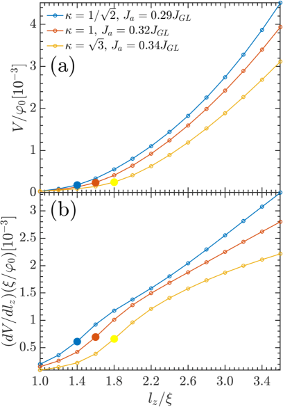
Figure 6: (a) Voltage across the $z$ direction as a function of the thickness of the sample for three values of $\kappa$: the value of $J_{a}$ for each case corresponds to the first critical current density when the resistive state sets in. The highlighted dots are the critical $l_{z,c}$ values for which the v-av pairs combine to make a closed vortex. (b) The derivative of the voltage: the dots separate the two regimes of straight to curved vortices; the inflection points coincide with $l_{z,c}$.

As we mentioned previously, as the thickness of the sample is increased, there is a crossover between straight to curved v-av pair. In what follows, we show a consistence between the criterion based on the aspect ratio of the vortex (antivortex) and an important physical quantity, namely, the voltage across the $z$ direction on the lateral side of the film; by aspect ratio, we mean the distance between the center of the vortex and the antivortex along the $y$ direction when their tips first touch each other. For this purpose, we calculate the time average of the following voltage:

$$U(t) = -\frac{2}{n_{x}}\sum_{i=n_{x}/2}^{n_{x}}\int_{0}^{l_{z}/2}\,E_{z}(x_{i},l_{y}/2,z)dz$$ (12)

$$= \frac{2}{n_{x}}\sum_{i=n_{x}/2}^{n_{x}}\int_{0}^{l_{z}/2}\frac{\partial A_{z}(x_{i},l_{y}/2,z)}{\partial t}dz,$$

where $n_{x}=l_{x}/\Delta x$, and $x_{i}=(i-n_{x}/2-1)\Delta x$ for all $\{i=1,2,\ldots,n_{x}+1\}$ are the $x$ coordinates of the mesh points. Here, we have not considered the branch $-l_{z}/2\leq z\leq 0$. By symmetry, had we included this contribution, the voltage would vanish.

When a closed vortex appears, we will have a larger contribution for the current flowing in the vertical direction, and consequently an increase in the voltage. For a fixed value of $\kappa$ and current density $J_{a}$, we determine the voltage for several values of $l_{z}$. We have done this for three distinct values of the Ginzburg-Landau parameter. The respective value of $J_{a}$ is chosen so as to correspond to the critical current density $J_{c1}$ for the lowest thickness, $l_{z}=1\xi$. The results are summarized in Fig. 6. In panel (a) we present the voltage as a function of the thickness of the film. We find that, at a certain point, which we denote by $l_{z,c}$, there is a change of the behavior of the $V(l_{z})$ curves. These points are highlighted in panel (a). They signal a crossover from linear to curved v-av pairs.

In order to make sure that this special point is correlated to the straight-to-curved vortex crossover, we calculate the derivative $dV(l_{z})/dl_{z}$ for the three values of $\kappa$ (see panel (b)). As can be seen, the derivatives have an inflection point which are highlighted in panel (b). These points correspond to $l_{z,c}$. We find the following critical values, $l_{z,c}=1.4\xi,1.6\xi,1.8\xi$ for $\kappa=1/\sqrt{2},1,\sqrt{3}$, respectively. We must emphasize that, first we determine the value of $l_{z,c}$ by inspecting the aspect ratio of the curvature of the vortex. Second, we check if the result is in agreement with inflection point of $dV(l_{z})/dl_{z}$. For all the three cases mentioned above they coincide.

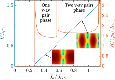
Figure 7: IV (blue line) and IR (red line) characteristic curves, respectively, for $\kappa=1$ and $l_{z}=3\xi$. The Meissner state (full superconductivity) survives up to $J_{a}=J_{c1}=0.27J_{GL}$. Above this current density, the resistive state sets in. The resistive state splits into two phases. In one of them the vortex and the antivortex nucleate only at the defects on the border of the superconductor. In the second phase, another set of v-av pairs nucleates at the frontiers between unit cells. The second jump in the IV characteristic is the signature of this crossover. The insets illustrate this scenario through the modulus of the order parameter in the $xy$ plane ($z=0$ plane).

Now we discuss the transport properties of the superconductor. The IV and IR characteristics are presented in Fig. 7 for $\kappa=1$ and $l_{z}=3\xi$. As we increase the applied current density, the system becomes unstable to the penetration of v-av pairs. When $J_{a}$ achieves the value $J_{c1}=0.27J_{GL}$ the superconductor goes to the resistive state, where a periodic formation v-av pairs occurs. Notice that $J_{c1}$ is smaller than the depairing current density $J_{GL}$. This is a consequence of the defects deliberately introduced at the border of the superconducting film. If we further increase $J_{a}$, a second jump appears in the IV curve at $J_{a}=0.575J_{GL}$. This is an indication that another two adjacent v-av pairs around the central one are nucleating (see insets). This is in correspondence with the experimental observations of multiple penetrations of kinematic vortices in Sn film by Sivakov et al. [24]. Finally, when the current density reaches the value $J_{a}=J_{c2}=1.155J_{GL}$ the superconductor goes straight to the normal state. We believe that for larger unit cells, additional jumps in the IV curve would occur.

III.4 Single Defect (Half-Closed Vortex)

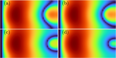
Figure 8: Color maps of the superconducting Cooper-pair density, $|\psi|$, for $\kappa=1$, $l_{z}=4\xi$, and $J_{a}=0.26J_{GL}$ throughout the plane $x=0$: (a) an av nucleates in the left edge of the sample and moves towards the opposite side; (b) the ends of the av touch the $y=l_{y}/2$ plane and form a half-closed vortex; (c) a half-closed vortex diminishing its radius; (d) the half-closed vortex shrinking down.

We also have considered a single defect in the middle of a unit cell (in the middle of front edge in Fig. 1). In this configuration, only an antivortex nucleates on the $y=-l_{y}/2$ surface. Once the antivortex nucleates at $y=-l_{y}/2$ it moves directly towards the opposite side. As can be seen from Fig. 8, as the antivortex approaches the other side of the sample, it becomes significantly curved (see panel (a)). When it reaches the surface $y=l_{y}/2$, surprisingly, it does not escape the sample. Instead, its ends touch the surface giving rise to a half-closed vortex (see panels (b) and (c)). Then, it diminishes its ratio until it collapses (see panel (d)).

Due to its intrinsic nature, it is very difficult to observe experimentally the closed vortex. In addition, both the closed and half-closed vortex are very unstable. Therefore, we require an indirect method that signals either a v-av or a single half-closed vortex curves. Having this in mind, we propose a setup to detect the curvature of the v-av pair when it gives rise to a closed vortex with a non vanishing aspect ratio. Instead of doing this for a closed vortex, which is formed inside the sample, we think it should be much easier for a half-closed vortex, since its collapse occurs on the surface. For this purpose, we calculate the time average of the of the magnetic flux on the lateral side of the film. In order to calculate the magnetic flux, we focus in a small region where the antivortex tips touch the plane $y=l_{y}/2$, although we could extend it throughout the whole lateral side of the unit cell. We evaluate the following equation:

$$\Phi(t)=\int_{0}^{l_{z}/2}\int_{-\xi}^{\xi}\,h_{y}(x,\pm l_{y}/2,z)\,dxdz.$$ (13)

Here, the minus sign stands for the left edge where the antivortex nucleates, and the plus sign is for the opposite one where the antivortex ends touch the surface. We consider only half of the lateral edge, otherwise the total flux would vanish.

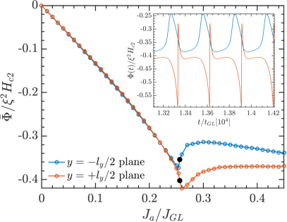
Figure 9: The main panel presents the time average of the magnetic flux, $\bar{\Phi}$, across the surfaces defined in Eq. 13; the black points correspond to the beginning of the resistive state. The inset shows the magnetic flux, $\Phi$, as a function of time. The parameters used were $\kappa=1$, $l_{z}=4\xi$, and $J_{a}=0.26J_{GL}$.

Fig. 9 presents the results for the time averaged magnetic flux by using the same parameters as those used in Fig. 8. As can be clearly seen, until the transition to the resistive state, the flux is approximately the same through both surfaces $y=\pm l_{y}/2$. Nevertheless, once the resistive state sets in, they become different as much as $\Delta\bar{\Phi}\approx 0.09\xi^{2}H_{c2}\approx 0.02\Phi_{0}$. This is signaling that the antivortex is piercing the $y=+l_{y}/2$ surface. Therefore, for this to happen, the antivortex necessarily has to bend.

Since the creation and annihilation of the half-closed vortex is a dynamical process, the flux evolves periodically. The AC magnetic flux can be seen in the inset of Fig. 9. The period of the AC signal depends on the applied current density. For $J_{a}=0.26J_{GL}$ we find that the period is $\tau\approx 0.03\times 10^{4}t_{GL}$. For low-$T_{c}$ materials like Nb films [23], $t_{GL}\approx 6.72$ ps. This produces $\tau\approx 2$ ns, which is in the GHz frequency range.

As we can see, the measurement of the difference between the time averaged magnetic flux threading at each plane, as displayed in Fig. 9, can be an indirect method for the experimental detection of a closed vortex. Such measurement is experimentally feasible by using the recently developed nanoSQUIDs [25, 26, 27], which are capable of detecting the variation of the flux produced by the closed vortex in the time and length scale we used in our computations.

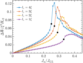
Figure 10: Difference between the average magnetic flux on both sides of the sample through two vertical circuits positioned on the planes $y=\pm(l_{y}/2+\xi)$. The domain of the circuits is given by $\{-\xi\leq x\leq\xi,\,-l_{z}/2\leq z\leq L_{z}/2\}$. The value of $L_{z}$ was chosen such that the area of the circuit above the $z=l_{z}/2$ surface is the same for all thicknesses $l_{z}$. The points just before the onset of the resistive state are highlighted in black.

We must emphasize that for thin superconductors, the measurement of the flux in the region prescribed in the above setup can be experimentally challenging. For this reason, we also present another indirect method for the detection of a closed vortex. Fig 10 shows the difference between the averaged magnetic flux calculated at the lateral sides of our superconductor as a function of the applied current density, for different superconductor thicknesses. In contrast with the previous case, here the flux is calculated from the bottom of the superconductor up to a height well above the sample surface. The flux is evaluated across a vertical rectangular surface, located a coherence length away from the lateral surface. This makes the proposed experiment much more feasible.

The black dots in Fig. 10 represent the onset of the resistive state for each thickness. We are interested in current densities slightly above these values. In this region, the antivortex moves through the whole sample, being expelled at the other side (animations of this regime, as well as the one described below, can be found in the Supplement Material ). Due to its curvature, the antivortex produces a larger magnetic flux in the plane which it is moving into, increasing the flux difference between each plane. Since the curvature increases with the film thickness, this difference also increases with the sample thickness, as shown in Fig. 10. Nevertheless, for large values of the current density, a vortex also penetrates the superconductor at the opposite side, with the pair being annihilated inside the sample, reducing the impact of the curvature in the flux. The penetration of this vortex becomes easier as the superconductor thickness increases, which explains why the flux difference for $l_{z}=4\xi$ is smaller than for $l_{z}=2\xi$ or $3\xi$ at high current densities, for example. In summary, by comparing the magnetic flux difference, at the onset of the resistive state, for films with different thicknesses, we can clearly demonstrate the existence of the half-closed vortex. Given the inherent complexity for the direct observation of a closed vortex, our indirect method brings a new possibility for the first detection of such objects.

IV Concluding remarks

To summarize, we have shown that the combination of the flux lines of a vortex and an antivortex during their annihilation gives origin to a closed vortex loop. As we show here, the formation of the closed vortex depends on how easily the flux lines can be bent due to the action of the applied current, with this bending increasing with the superconducting film thickness and decreasing with the Ginzburg-Landau parameter $\kappa$. Since the motion and annihilation of vortices are highly dissipative processes, understanding their behavior is of fundamental importance to the design of electronic devices.

Our findings suggest a new method to experimentally observe a closed vortex. As discussed here, closed vortices can be indirectly detected by the measuring the flux produced by their stray fields. We emphasize that the recently developed nanoSQUIDs are capable of performing such measurements in the time and length scales that our system requires.