A JWST/NIRSpec Exploration of the Connection between Ionization Parameter, Electron Density, and Star-Formation-Rate Surface Density in $z=2.7-6.3$ Galaxies

Abstract

We conduct a statistical analysis of the key factors responsible for the variation in the ionization parameter ($U$) of high-redshift star-forming galaxies based on medium resolution JWST/NIRSpec observations obtained by the Cosmic Evolution Early Release Science (CEERS) survey. The sample consists of 48 galaxies with spectroscopic redshifts $z=2.7-6.3$ which are largely representative of typical star-forming galaxies at these redshifts. The [S II] $\lambda\lambda 6718,6733$ doublet is used to estimate electron densities ($n_{e}$), and dust-corrected H$\alpha$ luminosities are used to compute total ionizing photon rates ($Q$). Using composite spectra of galaxies in bins of [O III] $\lambda\lambda 4960,5008$/[O II] $\lambda\lambda 3727,3730$ (i.e., O32) as a proxy for $U$, we determine that galaxies with higher O32 have $\langle n_{e}\rangle\simeq 500$ cm^-3 that are at least a factor of $\simeq 5$ larger than that of lower-O32 galaxies. We do not find a significant difference in $\langle Q\rangle$ between low- and high-O32 galaxies. We further examine these results in the context of radiation- and density-bounded nebulae, and use photoionization modeling of all available strong rest-frame optical emission lines to simultaneously constrain $U$ and oxygen abundance ($Z_{\rm neb}$). We find a large spread in $\log U$ of $\approx 1.5$ dex at a fixed $Z_{\rm neb}$. On the other hand, the data indicate a highly significant correlation between $U$ and star-formation-rate surface density ($\Sigma_{\rm SFR}$) which appears to be redshift invariant at $z\sim 1.6-6.3$, and possibly up to $z\sim 9.5$. We consider several avenues through which metallicity and $\Sigma_{\rm SFR}$ (or gas density) may influence $U$, including variations in $n_{e}$ and $Q$ that are tied to metallicity and gas density, internal dust extinction of ionizing photons, and the effects of gas density on the volume filling fraction of dense clumps in H II regions and the escape fraction of ionizing photons. Based on these considerations, we conclude that gas density may play a more central role than metallicity in modulating $U$ at these redshifts.

I. Introduction

The ionization parameter ($U$)—commonly defined as the ratio of the number density of incident ionizing photons and the number density of hydrogen atoms—is a key property of the interstellar medium (ISM) that depends on the intensity and hardness of the ionizing radiation field, gas density, and the spatial distribution of gas relative to ionizing sources. Accordingly, variations in $U$ can provide meaningful insights into how the ISM and ionizing sources evolve with redshift and/or galaxy properties. Recent observations with the James Webb Space Telescope (JWST) have revealed the presence of galaxies with apparently “extreme” ionization conditions at the epoch of reionization, where $U$ may be an order of magnitude or more larger than that of typical star-forming galaxies at lower redshifts (Tang et al., 2023; Bunker et al., 2023). The strong inverse correlation between $U$ and oxygen abundance ($Z_{\rm neb}$) seen in the local Universe (Dopita & Evans, 1986; Pérez-Montero, 2014) is commonly interpreted as a reflection of the harder ionizing spectra associated with low metallicity stars. Consequently, the large values of $U$ seen at high redshift are ostensibly due to the lower metallicity stellar populations characteristic of galaxies at these redshifts. While these results are intriguing, they also motivate a more detailed investigation of the physical causes of the elevated $U$ inferred for high-redshift galaxies.

In this context, there have been a number of efforts focused on explaining the redshift evolution of $U$ at a fixed stellar mass up to $z\sim 2$. Early work suggested that this evolution reflects the decrease in metallicity (and implied increase in hardness of the ionizing spectrum) of galaxies with redshift at a given stellar mass (e.g., Sanders et al. 2016a; Kashino & Inoue 2019). On the other hand, because $U$ is sensitive to the total ionizing photon rate (or SFR), the increase in SFR with redshift at a fixed stellar mass has also been invoked to explain in part the elevated $U$ seen at high redshift (e.g., Kaasinen et al. 2017). Others have pointed to the increased gas (or SFR) surface densities and/or higher electron densities ($n_{e}$) as a possible factor in the redshift evolution of $U$ (Brinchmann et al., 2008; Liu et al., 2008; Shimakawa et al., 2015; Masters et al., 2016; Bian et al., 2016; Davies et al., 2021; Papovich et al., 2022; Reddy et al., 2023b). Previous studies have necessarily been limited in the redshift range over which one can robustly constrain $U$ and $n_{e}$, since the lines typically used to infer them for the same galaxies are inaccessible from the ground above $z\sim 4$.

The James Webb Space Telescope (JWST) now allows access to the same diagnostics of $U$, $Z_{\rm neb}$, and $n_{e}$ for galaxies well into the epoch of reionization, where these properties are expected to lie outside the ranges typically observed up to $z\sim 2-3$, but which still overlap with the more “extreme” sources (i.e., with high $U$, low $Z_{\rm neb}$, and high $n_{e}$) at these lower redshifts. Such measurements over larger dynamic ranges in redshift, stellar characteristics, and physical conditions in the ISM form an ideal dataset to evaluate the evolution in $U$. Here, we take advantage of public JWST/NIRSpec spectroscopy obtained as part of the Cosmic Evolution Early Release Science (CEERS) survey to identify the factors responsible for modulating $U$ in high-redshift ($z=2.7-6.3$) galaxies.

The paper is organized as follows. The data, line measurements, and construction of composite spectra are discussed in Section II. The empirical relationship between $U$ and both $n_{e}$ and $Q$ are presented in Section III, and these results are discussed in the context of radiation- and density-bounded nebulae in Sections IV.1 and IV.2. In Sections IV.3 and IV.4, we consider several pathways through which metallicity and SFR surface density, respectively, may affect $U$. Our conclusions and suggestions for future work are presented in Section V. A Chabrier (2003) initial mass function (IMF) is considered throughout the paper. Wavelengths are reported in the vacuum frame. We adopt a cosmology with $H_{0}=70$ km s^-1 Mpc^-1, $\Omega_{\Lambda}=0.7$, and $\Omega_{\rm m}=0.3$.

II. Data and Measurements

We used the publicly available NIRSpec Multi Shutter Assembly (MSA) data from the CEERS program (Program ID: 1345; Finkelstein et al. 2022; Finkelstein et al., in prep.; Arrabal Haro et al, in prep.) for this analysis. A total of 318 unique objects in the AEGIS field were targeted using grating and filter combinations that yielded medium resolution ($R\sim 1000$) spectroscopy at $\lambda=1-5$ $\mu$m, with an integration of $\simeq 52$ min per grating and filter combination. The NIRSpec data were reduced following the procedures described in Shapley et al. (2023b), Sanders et al. (2023a), and Reddy et al. (2023a). The JWST calwebb_detector1 pipeline was used to process individual uncalibrated exposures, correcting for saturated pixels, subtracting bias and dark current, and masking other artifacts resulting from cosmic ray hits. Flatfielding, background subtraction, and wavelength solutions were applied to the 2D spectrograms. These spectrograms were then combined using offsets appropriate for the three-point nod dither pattern. One-dimensional spectra were optimally extracted from the spectrograms, as described in Sanders et al. (2023a). If no emission lines or continua were visible, then an extraction was not performed. One-dimensional spectra were extracted for 252 targets. Slit loss corrections and a final flux scaling were applied to force the integrated fluxes from the spectra to agree with the broadband photometry, details of which can be found in Reddy et al. (2023a) and Sanders et al. (2023a).

Emission line fluxes were measured by fitting the line profiles with Gaussian functions, along with a continuum model determined by the best-fit SED, thus accounting for stellar absorption under the H I emission lines (see Sanders et al. 2023a for further details). Most of the analysis presented here relies on composite spectra that were generated by shifting each object’s spectrum to the rest frame, converting from flux density to luminosity density, interpolating to a common wavelength grid, and averaging luminosity densities at each wavelength point using $3\sigma$ clipping. Average line luminosities, line ratios, and their corresponding uncertainties including sample variance were calculated by generating many realizations of the composite spectra. In each realization, the spectra of individual objects were perturbed according to their measurement errors, and composite spectra were constructed by random selection of these perturbed spectra with replacement. Line flux measurements on the composite spectra were performed in a manner similar to that of individual objects. All line ratios presented here were corrected for dust attenuation based on the Balmer decrement ($\text{H$\alpha$}/\text{H$\beta$}$) and/or the higher-order Balmer lines (H$\gamma$ and H$\delta$) for individual objects or from the composite spectra, assuming the Cardelli et al. (1989) Milky Way extinction curve. This extinction curve has been shown to apply to typical star-forming galaxies at high redshift (Reddy et al., 2020). The line diagnostics presented in this study are listed in Table 1, but all available rest-frame optical emission lines were used in the photoionization modeling discussed in Section IV.3.

Table 1Line Diagnostics

Line Diagnostic	Definition
O3	$\text{[{O~{}III}]}5008/\text{H$\beta$}$
O32	$\text{[{O~{}III}]}4960+5008/\text{[{O~{}II}]}3727+3730$
N2	$\text{[{N~{}II}]}6585/\text{H$\alpha$}$
S2	$\text{[{S~{}II}]}6718+6733/\text{H$\alpha$}$
Ne3O2	$\text{[{Ne~{}III}]}3870/\text{[{O~{}II}]}3727+3730$
R23	$(\text{[{O~{}III}]}4960+5008\,+\text{[{O~{}II}]}3727+3730)/\text{H$\beta$}$

As described in Shapley et al. (2023b), the broadband photometry of galaxies in the sample was corrected for the contribution from strong emission lines and then fit with the stellar population synthesis models of Conroy et al. (2009) using the FAST program (Kriek et al., 2009). Delayed-$\tau$ star-formation histories were adopted, where ${\rm SFR}(t)\propto t\times\exp(-t/\tau)$, with a minimum age of $10$ Myr. Galaxies were fit using two sets of assumptions: the SMC extinction curve (Gordon et al., 2003) and a subsolar stellar metallicity ($Z_{\ast}=0.004$), and the Calzetti et al. (2000) attenuation curve and a $\sim$solar metallicity ($Z_{\ast}=0.02$) for the redshift and stellar mass criteria given in Shapley et al. (2023b). For the purposes of this analysis, we focused on the stellar population ages and stellar masses derived from the fitting, which are similar to those obtained for the Binary Population and Stellar Synthesis (BPASS; Eldridge et al. 2017; Stanway & Eldridge 2018) models that we consider Section IV.3.2.

The final sample used in this study was assembled as follows. First, galaxies were required to have secure spectroscopic redshifts $z_{\rm spec}=2.7-6.3$, reducing the sample from 252 objects with extracted spectra to 110. The lower redshift corresponds to the limit of ground-based spectroscopic studies of electron densities based on [S II] $\lambda\lambda 6718,6733$, the tracer used in this study. The upper redshift corresponds roughly to the limit where [S II] is accessible with JWST/NIRSpec. Second, AGN that were identified with $\text{[{N~{}II}]}/\text{H$\alpha$}\geq 0.5$ or significant broad components to their emission lines were excluded, resulting in 106 remaining objects. Third, we required $\geq 3\sigma$ detections of [O II] $\lambda\lambda 3727,3730$, H$\beta$, [O III] $\lambda\lambda 4960,5008$, and H$\alpha$ to ensure robust dust corrections and O32, yielding 54 galaxies. Finally, 6 galaxies which had noisy photometry, thus rendering it difficult to obtain robust estimates of stellar population properties (e.g., age, reddening, stellar mass, SFR), were removed from the sample. The final sample includes 48 galaxies with the redshift distribution and SFR and $M_{\ast}$ shown in Figure 1. As discussed in Shapley et al. (2023b), the bulk of the sample is representative of star-forming galaxies at $z\lesssim 5$, while above this redshift the galaxies generally have higher specific SFRs relative to typical star-forming galaxies (at fixed mass) at those redshifts.

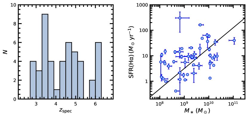
Figure 1.— Left: Spectroscopic redshift histogram of the 48 galaxies in the sample. Right: Distribution of H$\alpha$-based SFRs and $M_{\ast}$ for the 48 galaxies in the sample. The mean relation between SFR and $M_{\ast}$ at $z\sim 4.4$ (roughly the mean redshift of the sample) is indicated by the solid line (Shapley et al., 2023b).

III. Electron Density and Ionizing Photon Rate

For a radiation-bounded (spherical) nebula, the ionization parameter ($U$) is related to the ionizing photon rate ($Q$), hydrogen density ($n_{\rm H}$), and Strömgren radius ($R_{\rm S}$):

$$U\propto\frac{Q}{n_{\rm H}R_{\rm S}^{2}}.$$ (1)

The Strömgren radius is also related to $Q$ and the volume-averaged hydrogen density, $\langle n_{\rm H}\rangle$:

$$R_{\rm S}^{3}\propto\frac{Q}{\langle n_{\rm H}\rangle^{2}}\propto\frac{Q}{\epsilon n_{\rm H}^{2}},$$ (2)

where the volume filling factor $\epsilon=(\langle n_{\rm H}\rangle/n_{\rm H})^{2}$. This factor represents the fraction of the H II region volume containing denser material that dominates the emission-line fluxes, such as [S II] (Osterbrock & Flather, 1959; Kennicutt, 1984). Combining Equations 1 and 2, and assuming all the gas is ionized (i.e., $n_{\rm H}\sim n_{e}$, where $n_{e}$ is the electron density), then yields the following dependence of $U$ on $Q$, $n_{e}$, and $\epsilon$:

$$U\propto[Qn_{e}\epsilon^{2}]^{1/3}.$$ (3)

Note that $U$ is commonly defined as the ratio of the number density of ionizing photons over the number density of hydrogen atoms. For a radiation-bounded nebula, the number density of ionizing photons is simply proportional to the photon flux received at the surface of a sphere with radius $R_{S}$. An increase in density results in lower $R_{S}$ and hence a higher photon flux. Thus, the overall dependence for a radiation-bounded nebula is one where $U$ increases with $n_{\rm H}$ (or $n_{e}$). Motivated by the theoretical dependencies in Equation 3, we first examined how $U$ varies with both $Q$ and $n_{e}$. The photoionization modeling used to determine $U$ is discussed in Section IV. For the moment, however, we consider the O32 ratio as a proxy for $U$. The ratio of [S II] $\lambda 6718$ and [S II] $\lambda 6733$, $R(\text{{S~{}II}})$, was used to infer $n_{e}$ using the relation from Sanders et al. (2016a).

The ionizing photon rate ($Q$) depends on the SFR and the ionizing photon rate per unit SFR, or the ionizing production efficiency, $\xi_{\rm ion}$ (Robertson et al., 2013; Bouwens et al., 2016; Shivaei et al., 2018; Theios et al., 2019; Reddy et al., 2022), such that $Q\propto\xi_{\rm ion}\times{\rm SFR}$. The ionizing production efficiency depends on the properties of massive stars, such as their stellar metallicity, age, whether they evolve as single stars or binaries, and the IMF. For this analysis, $Q$ is determined empirically from the dust-corrected H$\alpha$ luminosity assuming the relationship of Leitherer & Heckman (1995) and no escape or dust absorption of ionizing photons. We consider the case of a non-zero escape fraction of ionizing photons from H II regions in Section IV.2, and dust absorption of ionizing photons in Section IV.3.4.

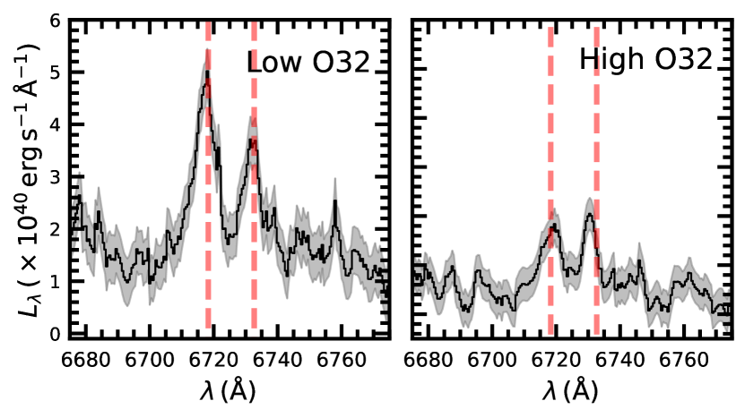
Figure 2.— [S II] $\lambda\lambda 6718,6733$ in the composite spectra of the low- and high-O32 bins (left and right, respectively), each containing $N=24$ galaxies. The $1\sigma$ measurement uncertainty is indicated by the grey shaded regions.

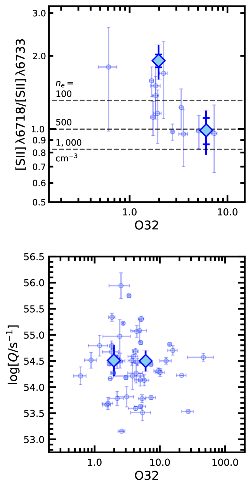
Figure 3.— Variation of $R(\text{{S~{}II}})$ (top) and $\log[Q/{\rm s^{-1}}]$ (bottom) with O32. Individual galaxies with detections of [S II] and $Q$ measurements are indicated by small circles in the top and bottom panels, respectively. Mean measurements from composite spectra of galaxies are shown by the diamonds. Measurement uncertainties for individual and composite values are indicated by the capped vertical lines. Estimates of sample variance (including measurement error) for the composite values are indicated by the uncapped vertical lines. In some cases, the error bars are smaller than the symbols.

Table 2O32 Subsamples

O32 bin	$N_{\rm comp}$	$\langle z\rangle$	$\langle{\rm O32}\rangle$	$\langle R(\text{{S~{}II}})\rangle$	$\langle\log[Q/{\rm s^{-1}}]\rangle$
all	48	$4.373$	$3.457\pm 0.074$	$1.355\pm 0.100$ ($0.303$)	$54.50\pm 0.01$ ($0.09$)
low	24	$4.063$	$1.978\pm 0.057$	$1.910\pm 0.116$ ($0.312$)	$54.51\pm 0.02$ ($0.15$)
high	24	$4.683$	$6.055\pm 0.174$	$0.987\pm 0.123$ ($0.204$)	$54.50\pm 0.02$ ($0.10$)

Owing to the relatively low $S/N$ of the [S II] doublet in the spectra of individual galaxies, we primarily limit our discussion to the results obtained from composite spectra, though for reference individual measurements are included in Figure 3—these individual measurements are obtained for the 12 (of 48) objects in the sample where both lines of the [S II] doublet are detected at $\geq 3\sigma$. To maximize the signal-to-noise of the composite spectrum, and in light of the absence of strong evolution in the ionization conditions in the ISM between $z\sim 2$ and $z\sim 6$ (Sanders et al., 2023a), composite spectra were constructed using galaxies over the full range of redshift ($z\sim 2.7-6.3$) of the sample.

Based on the composite spectrum of all 48 galaxies, we find $\langle R(\text{{S~{}II}})\rangle=1.355\pm 0.100$, corresponding to $\langle n_{e}\rangle=64_{-63}^{+84}$ cm^-3 (Table 2). This is somewhat lower than the $n\simeq 250$ cm^-2 derived for more massive star-forming galaxies at $z\sim 2.3$ (with a median stellar mass of $M_{\ast}\simeq 10^{10}$ $M_{\odot}$) from the MOSFIRE Deep Evolution Field (MOSDEF) survey (Sanders et al., 2016a). The mean electron density found here is also lower than the $n_{e}\gtrsim 300$ cm^-3 derived for individual galaxies at $z=4.0-8.7$ from the line-spread-function deconvolution of [O II] $\lambda\lambda 3727,3730$ by Isobe et al. (2023), where [O II] is not resolved for most of the objects in their sample. Five of the galaxies in their analysis are also in our sample. At face value, the sample-averaged lower $\langle n_{e}\rangle$ found here may be due to higher fraction of galaxies in our sample with lower $n_{e}$. A larger sample of galaxies with $n_{e}$ measured from the same feature (i.e., [S II] or [O II]) should help to clarify the source of this difference.

Composite spectra were also constructed in two equal-number bins of O32. The [S II] doublet in the composite spectra for the low- and high-O32 bins is shown in Figure 2. Properties of these bins, and the mean O32 and $R(\text{{S~{}II}})$ measured from the composite spectra, are listed in Table 2. The mean O32 and $R(\text{{S~{}II}})$ measured from the composite spectra are shown in Figure 3. The data reveal a potential correlation between $R(\text{{S~{}II}})$ and O32, or an inverse correlation between $n_{e}$ and O32. Specifically, the difference in $\langle R(\text{{S~{}II}})\rangle$ between the two O32 bins is significant at the $5.5\sigma$ level. The differences in $\langle R(\text{{S~{}II}})\rangle$ between the O32 bins suggest that $\langle n_{e}\rangle$ increases with O32: in this case, galaxies with $\langle{\rm O32}\rangle\simeq 6$ have $\langle n_{e}\rangle\simeq 500$ cm^-3, a factor of at least $\simeq 5\times$ larger than the $\langle n_{e}\rangle$ inferred for galaxies with $\langle{\rm O32}\rangle\simeq 2$. A similar trend of increasing $n_{e}$ with O32, and hence $U$, has been noted locally (Bian et al., 2016; Jiang et al., 2019) and at $z\sim 2-3$ (Shirazi et al., 2014; Reddy et al., 2023b), and inferred at $z\sim 1.1-2.3$ (Papovich et al., 2022). Our results suggest that such a trend continues unabated up to $z\sim 6.3$.

While these results imply a significant correlation between $n_{e}$ and O32, an accounting of sample variance (Section II) implies a rather large scatter in this correlation. In other words, there are some realizations of the sample—obtained by constructing composites of randomly selected objects with replacement—that result in $\langle R(\text{{S~{}II}})\rangle$ that are not significantly different between the low and high O32 bins. Likewise, there are some sample realizations where the difference in $\langle R(\text{{S~{}II}})\rangle$ between the low and high O32 bins is highly significant. The combined effects of measurement uncertainty and sample variance imply a $\simeq 2.5\sigma$ difference in $\langle n_{e}\rangle$ between the low- and high-O32 populations.

We now turn to the variation of $Q$ with O32 (bottom panel of Figure 3). A Spearman correlation test on the individual measurements for all 48 galaxies in the O32 sample implies a $p=0.67$ probability that the relationship between $\log[Q/{\rm s^{-1}}]$ and O32 occurs by random chance if the two parameters are uncorrelated with each other. The mean $\log[Q/{\rm s^{-1}}]$ measured in two equal-number bins of O32 are listed in Table 2 and shown by the large diamonds in the bottom panel of Figure 3. We find no significant difference in $\langle\log[Q/{\rm s^{-1}}]\rangle$ between the low- and high-O32 populations.

To summarize, we find evidence for increased $n_{e}$ among galaxies with higher O32 (though with large scatter), suggesting that variations in $n_{e}$ may play a role in the elevated ionization parameters inferred for high-redshift galaxies. On the other hand, we find no significant correlation between $Q$ and O32. These results are discussed further in the next section.

IV. Results and Discussion

In the previous section, we presented evidence suggesting that variations in $n_{e}$ may partly explain the high O32 (and $U$) inferred for high-redshift galaxies, while $Q$ does not appear to be an important factor in driving high O32 within the sample. Here, we examine these possibilities in the context of radiation- and density-bounded nebulae (Sections IV.1 and IV.2). These results are discussed in the context of previous studies that have addressed the roles of metallicity (Section IV.3) and SFR surface density (Section IV.4) in modulating $U$ at high redshift.

IV.1. Expectations for a Radiation-bounded Nebula

For a radiation-bounded nebula, we expect $U\propto Q^{1/3}n_{e}^{1/3}$ (Equation 3). In this case, the increase in $\langle n_{e}\rangle$ from the low-density regime ($n_{e}\sim 1-10$ cm^-3) for the low-O32 population to $n_{e}\simeq 500$ cm^-3 for the high-O32 population is expected to yield a factor of $\simeq 4-8$ increase in $\log U$, or a similar factor increase in O32. This expected increase in O32 due to changes in $n_{e}$ is more than sufficient to account for the factor of $\approx 3$ increase in $\langle{\rm O32}\rangle$ between the low- and high-O32 populations (Table 2). This also suggests that the nebulae are reasonably approximated as radiation bounded; $U$ will scale inversely with gas density for a density-bounded nebula (Section IV.2), which is inconsistent with the inferred increase in $U$ with $n_{e}$ (Figure 3). As there is no significant change in $\langle Q\rangle$ between the two O32 bins, the increase in O32 within these redshift bins is likely to be driven at least in part by an increase in $n_{e}$.

While $Q$ does not appear to be a significant factor in driving O32 within the sample, this does not preclude the possibility of a connection between $Q$ and $U$. In particular, Reddy et al. (2023b) suggest that the combined effects of an increasing $n_{e}$ and SFR (or $Q$) may be responsible for explaining the evolution towards higher $U$ from $z\sim 0$ to $z\sim 2$ at a fixed stellar mass (see also Brinchmann et al. 2008; Shirazi et al. 2014; Bian et al. 2016; Kaasinen et al. 2017; Papovich et al. 2022; Reddy et al. 2023b). The lack of a significant correlation between $Q$ and O32 found here may simply reflect the limited dynamic range in SFR probed by our sample (but see Section IV.2). The factor(s) driving the changes in $n_{e}$ and $Q$ are discussed in Section IV.4.

IV.2. Expectations for a Density-bounded Nebula

Rest-frame far-UV spectroscopic observations imply that typical galaxies at $z\sim 2-3$ have an ISM configuration where most sightlines are radiation bounded, while the remaining fraction of sightlines coincide with low-column-density or ionized (density-bounded) channels (Reddy et al., 2016; Steidel et al., 2018; Reddy et al., 2022). A low covering fraction of radiation-bounded sightlines will result in higher O32 even for a fixed intensity or hardness of the input (stellar) ionizing spectrum (e.g., Giammanco et al. 2005; Brinchmann et al. 2008; Nakajima et al. 2013). There are at least three consequences of such a configuration. First, there will be a non-zero fraction of ionizing photons that escapes the ISM. Second, O32 will overestimate $U$. For example, an H II region with a $50\%$ escape fraction of ionizing photons ($f_{\rm esc}$) would result in an order-of-magnitude overestimate of $U$ compared to a region with zero escape fraction (Giammanco et al., 2005). Third, in the limit where the covering fraction of radiation-bounded sightlines falls to zero (i.e., a purely density-bounded nebula), $R_{\rm S}$ will simply represent the physical extent of the cloud and it will not depend on $n_{e}$. As a result, $U$ will be inversely proportional to $n_{e}$ (Equation 1). Of course, real galaxies are unlikely to be purely density bounded and, as a consequence, one would expect $U$ to transition from a $n_{e}^{1/3}$ dependence to a close to $n_{e}^{-1}$ dependence as $f_{\rm esc}$ increases from $f_{\rm esc}=0$ to close to unity.

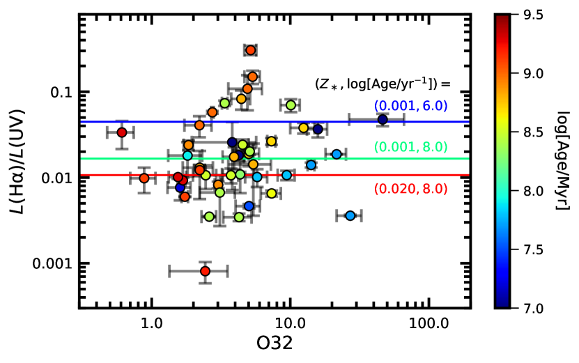
Figure 4.— Variation of $\text{$L$(H$\alpha$)}/L({\rm UV})$ with O32. Points are color coded by the best-fit stellar population age derived from SED fitting (Section II). Horizontal lines indicate the $\text{$L$(H$\alpha$)}/L({\rm UV})$ expected for the BPASS v2.2.1 binary constant-star-formation models for the indicated $Z_{\ast}$ and age.

It is prudent to investigate whether elevated $U$ (or O32) may be tied to a high $f_{\rm esc}$. An increase in $f_{\rm esc}$ suppresses H I recombination line fluxes relative to the non-ionizing UV continuum. If high escape fractions are responsible for driving elevated O32 ratios, one might expect the ratio of the (dust-corrected) H$\alpha$ and UV luminosities, $\text{$L$(H$\alpha$)}/L({\rm UV})$, to anti-correlate with O32. Figure 4 shows the variation of $\text{$L$(H$\alpha$)}/L({\rm UV})$ with O32 for the 43 objects in the sample with well-constrained SED fits around $1500$ Å, and thus robust $L({\rm UV})$ determinations. The data do not indicate that galaxies with higher O32, in particular those with ${\rm O32}>10$, have systematically lower $\text{$L$(H$\alpha$)}/L({\rm UV})$.

However, it is important to keep in mind that $\text{$L$(H$\alpha$)}/L({\rm UV})$ is also sensitive to the stellar metallicity ($Z_{\ast}$), IMF, and age of the stellar population. The variation in $\text{$L$(H$\alpha$)}/L({\rm UV})$ arising from stellar population differences (e.g., different $Z_{\ast}$ and age) for the Binary Population and Stellar Synthesis (BPASS; Eldridge et al. 2017; Stanway & Eldridge 2018) v2.2.1 constant-star-formation (CSF) models with an upper-mass cutoff of the IMF of $100$ $M_{\odot}$ is illustrated in Figure 4. Galaxies with lower stellar metallicities and younger ages will exhibit higher intrinsic $\text{$L$(H$\alpha$)}/L({\rm UV})$. Indeed, the stellar population ages derived from fitting the broadband SEDs of galaxies in the sample (Section II; Shapley et al. 2023b) are systematically younger for those with higher O32, as indicated by the color-coding in Figure 4. If galaxies with high O32 are preferentially undergoing a burst of star formation, and such a burst is accompanied by a high $f_{\rm esc}$ due to an increase in ISM porosity related to feedback (e.g., Trebitsch et al. 2017; Kimm et al. 2019; Ma et al. 2020; Kakiichi & Gronke 2021), then the deficit of $L$(H$\alpha$) relative to $L({\rm UV})$ expected for a non-zero escape fraction may be masked by the higher intrinsic $L$(H$\alpha$) relative to $L({\rm UV})$ for a bursty (or young) low-metallicity galaxy.

We cannot conclusively rule out this possibility with the data at hand. An analysis of the gas covering fraction of galaxies with high O32 may elucidate the role of ionizing photon leakage in such galaxies. Nevertheless, invoking a very high $f_{\rm esc}$ to explain the high O32 observed for some galaxies (Giammanco et al., 2005; Brinchmann et al., 2008; Nakajima et al., 2013) necessarily implies that a large fraction of the gas must be ionized, which in turn would have the effect of suppressing star formation and the production of ionizing photons. A large representative sample of galaxies at $z\gtrsim 2.7$ may be required for obtaining statistically robust constraints on the O32 distribution and the duty cycle of a (presumably) transient and short phase of elevated O32 and high $f_{\rm esc}$ (e.g., Naidu et al. 2022).

Note that dust-corrected $L$(H$\alpha$) will underestimate $Q$ if there is a non-zero escape fraction of ionizing photons, or if there is significant dust extinction of ionizing photons within the H II regions (Section IV.3.4). It is possible that correcting for these effects may yield a more significant correlation between $Q$ and O32 (Figure 3), if the average escape fraction is increasing with O32. However, the expectation of such a correlation is complicated by the large scatter in $\log[Q/{\rm s^{-1}}]$ that may be driven by stellar population differences from galaxy to galaxy. The upshot is that it is difficult to use the $\text{$L$(H$\alpha$)}/L({\rm UV})$ ratio alone to distinguish galaxies that may be leaking a significant fraction of ionizing photons, and one should turn to other constraints in this regard (e.g., escape fraction and kinematics of Ly$\alpha$, gas covering fraction, etc.).

IV.3. Metallicity Considerations

The well-established anti-correlation between $U$ and $Z_{\rm neb}$ for local star-forming galaxies (e.g., Dopita & Evans 1986; Dopita et al. 2006; Pérez-Montero 2014) is typically interpreted as a reflection of the harder and more intense ionizing spectra associated with lower-metallicity massive stars (Dopita et al., 2006; Leitherer et al., 2014). If so, one would expect $U$ to be driven primarily by changes in $Z_{\rm neb}$. However, the hardness of the ionizing spectrum (which $U$ is sensitive to) is expected to correlate more directly with $Z_{\ast}$ than with $Z_{\rm neb}$, since the former is responsible for regulating stellar opacity and the absorption of ionizing photons by stellar winds (Dopita et al., 2006). Hence, investigating variations in $U$ with $Z_{\ast}$ presents a potentially more direct route to assessing the role of metallicity in modulating $U$ (Strom et al., 2018; Reddy et al., 2023b), particularly in cases where the Fe-sensitive $Z_{\ast}$ may differ from the O-sensitive $Z_{\rm neb}$ as is the case for the $\alpha$-enhanced stellar populations typical of $z\gtrsim 2$ galaxies (Steidel et al., 2016; Cullen et al., 2019; Topping et al., 2020b, a; Cullen et al., 2021; Runco et al., 2021; Reddy et al., 2022). As we discuss below, the relationship between $U$ and $Z_{\rm neb}$ is still relevant in determining the effects dust on the intensity and hardness of the ionizing radiation field. The expected dependence of $U$ on $Z_{\ast}$ is discussed below, but first we address the variation of $U$ with $Z_{\rm neb}$ within the sample.

The photoionization modeling used to simultaneously constrain $\log U$ and $\log[Z_{\rm neb}/Z_{\odot}]$ is described in Section IV.3.1. The effect of $Z_{\rm neb}$ and $Z_{\ast}$ on $U$ is discussed in Section IV.3.2. The possibility that metallicity may affect $n_{e}$ is addressed in Section IV.3.3, and we also consider the diminution and softening of the ionizing radiation field in dusty H II regions in Section IV.3.4. Section IV.3.5 addresses whether the stellar population synthesis models incorrectly predict how rapidly the hydrogen-ionizing spectrum hardens with decreasing metallicity below $Z_{\ast}\simeq 0.001$.

IV.3.1 Photoionization Modeling

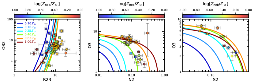
Figure 5.— O32 vs. R23 (left), and the N2 and S2 BPT diagrams (middle and right, respectively). Photoionization modeling predictions for how the line ratios vary with $\log U$ at fixed values of $Z_{\rm neb}$ are indicated by the colored curves. The modeling results shown here assume the fiducial BPASS model (i.e., a fixed ionizing spectrum), and we note that the curves are relatively insensitive to the assumed age and metallicity at $Z_{\ast}\lesssim 0.002$ (see text). Data points for galaxies where the relevant lines are detected with ${\rm S/N}\geq 3$ are color coded by the best-fit $\log[Z_{\rm neb}/Z_{\odot}]$ found from photoionization modeling of all the significantly-detected lines.

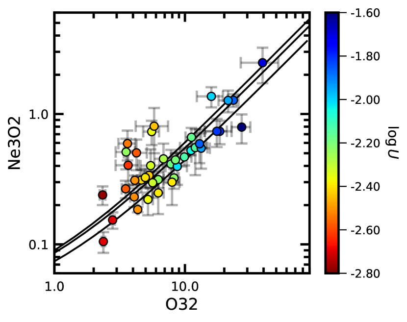
Figure 6.— Ne3O2 vs. O32 for the 40 objects in the sample where all the relevant lines are detected at $\geq 3\sigma$ (circles), color coded by the inferred $\log U$. The model predictions for how the line ratios vary with $\log U$ are denoted by the three black curves for three values of oxygen abundance: $\log[Z_{\rm neb}/Z_{\odot}]=-1.0,-0.5,0.0$.

Photoionization modeling was used to simultaneously determine $Z_{\rm neb}$ and $\log U$ using all available rest-frame optical emission lines, including [O II] $\lambda\lambda 3727,3730$, [Ne III] $\lambda 3870$, H$\delta$, H$\gamma$, H$\beta$, [O III] $\lambda\lambda 4960,5008$, [O I] $\lambda 6302$, H$\alpha$, [N II] $\lambda 6585$, and [S II] $\lambda 6718,6733$—the H I recombination lines aid in determining the “best-fit” value of nebular reddening, which is then used to correct all other lines for dust attenuation. The CLOUDY v17.02 radiative transfer code (Ferland et al., 2017) was used for the photoionization modeling, where $\log[Z_{\rm neb}/Z_{\odot}]$ was allowed to vary in the range $-2.0\leq\log[Z_{\rm neb}/Z_{\odot}]\leq 0.0$ in increments of 0.1 dex, and $\log U$ was allowed to vary in the range $-3.5\leq\log U\leq-1.0$ in increments of 0.1 dex. We further assumed an input ionizing spectrum corresponding to the BPASS v2.2.1 binary CSF model with $Z_{\ast}=0.001$, $\log[{\rm Age/Myr}]=8.0$, and an upper-mass cutoff of the IMF of $100$ $M_{\odot}$, values typical of those inferred based on fitting the BPASS models to the rest-frame far-UV spectra of star-forming galaxies at $z\sim 2-3$ (Steidel et al., 2016; Topping et al., 2020b; Reddy et al., 2022). In this subsequent discussion, we refer to this as the “fiducial” BPASS model. The hydrogen density was fixed to $n_{\rm H}=250$ cm^-3, similar to the average density inferred in Section III and in previous investigations of $z\sim 2$ galaxies (e.g., Sanders et al. 2016b; Topping et al. 2020a; Reddy et al. 2023b). Note that while we have argued that density plays a role in modulating $U$ (Section III), the $\log U$ inferred from photoionization modeling is relatively insensitive to the choice of $n_{\rm H}$ because the translation between O32 and $U$ is insensitive to $n_{\rm H}$ (see discussion in Reddy et al. 2023b). In other words, for a fixed set of measured line ratios, the inferred $U$ is relatively insensitive to the choice of $n_{\rm H}$, or, for that matter, the input ionizing spectrum over the range of stellar metallicity ($Z_{\ast}\lesssim 0.002$), age ($\log[{\rm Age/Myr}]=7.0-8.0$), and $n_{\rm H}$ ($n_{\rm H}\simeq 10-500$ cm^-3). Anywhere from 6 to 11 lines with ${\rm S/N}\geq 3$ were fit simultaneously for each object to constrain $Z_{\rm neb}$ and $U$. Uncertainties were determined from the dispersion of $Z_{\rm neb}$ and $U$ obtained by randomly perturbing the line fluxes by their errors many times and refitting the photoionization models to these realizations.

The efficacy of the models in reproducing line ratios sensitive to oxygen abundance ($Z_{\rm neb}$) is illustrated in Figure 5. Measured line ratios for galaxies where the relevant lines used to construct the ratios are detected with ${\rm S/N}\geq 3$ are color-coded by the best-fit $\log[Z_{\rm neb}/Z_{\odot}]$ obtained from the photoionization modeling. Of the 48 galaxies in the sample, 26 and 36 have upper limits on N2 and S2, respectively, and are therefore not shown in Figure 5. Naturally, these galaxies tend to have lower oxygen abundances based on their distribution of O32 and R23. The best-fit values can be compared with the model predictions of how the line ratios vary with $\log U$ at a fixed $Z_{\rm neb}$ (colored curves, where each curve represents a sequence in $\log U$ at a fixed $Z_{\rm neb}$). In almost all cases, the models are able to reproduce the measured line ratios within $3\sigma$. There are two objects (CEERS ID 2422 and 2693) where N2 and S2 indicate a higher $\log[Z_{\rm neb}/Z_{\odot}]\gtrsim-0.4$ than inferred from R23, $\log[Z_{\rm neb}/Z_{\odot}]\lesssim-0.8$. Additionally, the two objects (CEERS ID 2089 and 2514) with the highest inferred $Z_{\rm neb}$ in the sample (close to solar) are offset to lower R23 than the $Z_{\rm neb}=Z_{\odot}$ curve would predict for their O32—and similarly offset toward lower N2 than the $Z_{\rm neb}=Z_{\odot}$ curve would predict for their O3. A higher ($\gtrsim$solar) stellar metallicity and/or super-solar O/H may more appropriately describe these two galaxies. At any rate, the presence of the aforementioned objects in the sample does not alter the subsequent discussion or conclusions regarding the scatter in $\log U$ at a fixed $Z_{\rm neb}$.

Particularly tight constraints on $\log U$, with little dependence on $Z_{\rm neb}$, are afforded by the combination of O32 and Ne3O2 (e.g., Nagao et al. 2006; Pérez-Montero et al. 2007; Levesque & Richardson 2014; Steidel et al. 2016; Strom et al. 2017; Jeong et al. 2020; Shapley et al. 2023a). The latter is relatively insensitive to dust corrections owing to the wavelength proximity of [Ne III] $\lambda 3870$ and [O II] $\lambda\lambda 3727,3730$. Figure 6 displays the Ne3O2 and O32 measurements for the 40 galaxies in the sample where the line ratios could be measured (i.e., 8 of the 48 objects in the sample did not have $\geq 3\sigma$ detections of [Ne III]). Model predictions for Ne3O2 versus O32 are shown for the fiducial BPASS model and three values of $\log[Z_{\rm neb}/Z_{\odot}]=-1.0,-0.5,0.0$ (black curves). The average Ne3O2 measured in the low- and high-O32 bins are also indicated in the figure with the large diamonds. The measured line ratios are in excellent agreement with the model predictions and yield stringent constraints on $\log U$, with a typical uncertainty of $\simeq 0.1$ dex.

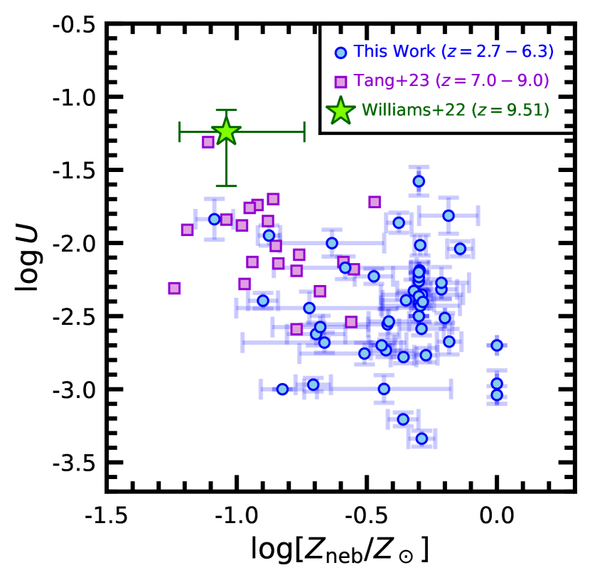
Figure 7.— $\log U$ vs. $\log[Z_{\rm neb}/Z_{\odot}]$ for the 48 galaxies in the sample (blue points). For comparison, the data from Tang et al. (2023) for $z=7.0-9.0$ galaxies (purple squares, error bars suppressed for clarity), and a lensed $z=9.51$ galaxy from Williams et al. (2022) (green star), are also shown.

IV.3.2 Variation of $U$ with $Z_{\rm neb}$ and $Z_{\ast}$

Figure 7 shows the distribution of $\log U$ and $\log[Z_{\rm neb}/Z_{\odot}]$ for the sample. A Spearman test indicates a high probability ($p=0.95$) of a null correlation between $\log U$ and $\log[Z_{\rm neb}/Z_{\odot}]$. Deeper observations of multiple abundance-sensitive line ratios (including those involving auroral lines such as [O III] $\lambda 4364$) should allow us to obtain more stringent constraints on $Z_{\rm neb}$ and reevaluate the significance of any correlation between $\log U$ and $\log[Z_{\rm neb}/Z_{\odot}]$. Note that the $\simeq 1$ dex order of magnitude dynamic range in $\log[Z_{\rm neb}/Z_{\odot}]$ probed by the sample may be insufficient to reveal the expected anti-correlation between $U$ and $Z_{\rm neb}$ given the large scatter between these quantities. For example, Sanders et al. (2020) and Topping et al. (2020a) do find a significant anti-correlation between these parameters when considering a larger dynamic range in $Z_{\rm neb}$. For comparison, data from Tang et al. (2023) for $z=7-9$ galaxies in CEERS, along with the $z=9.51$ lensed galaxy from Williams et al. (2022), are shown in Figure 7. The combination of these datasets suggests that galaxies with lower $Z_{\rm neb}$ have higher $U$, at least on average, similar to the behavior seen locally (Pérez-Montero, 2014).

In any case, it is clear that at a fixed $\log[Z_{\rm neb}/Z_{\odot}]\simeq-0.3$, there is a $\gtrsim 1.5$ order of magnitude variation in $\log U$ within our sample, which ranges from $\log U\simeq-3.3$ to $-1.6$, and is much larger than the typical $0.1-0.2$ dex measurement uncertainties in $\log U$. This large variation of $\log U$ at a fixed $Z_{\rm neb}$ has also been seen in lower-redshift ($z\sim 2$) galaxies, albeit over a smaller dynamic range in $Z_{\rm neb}$ (see Figure 10 of Topping et al. 2020a). The large spread in $U$ at a fixed $Z_{\rm neb}$ implies that factors other than $Z_{\rm neb}$ are driving the variation in $\log U$ within the sample.

As mentioned above, the metallicity dependence of $U$ can be more directly examined with estimates of $Z_{\ast}$. Using the BPASS models discussed above, Reddy et al. (2023b) evaluated the expected impact of changes in $Z_{\ast}$ on $U$. For example, $\log[\xi_{\rm ion}/{\rm s^{-1}/erg\,s^{-1}\,Hz^{-1}}]=25.39$ for the fiducial BPASS model. Given the evolution of decreasing metallicity with redshift (e.g., at a fixed mass), one would expect the $z>2.7$ galaxies in our sample to have stellar metallicities similar to or less than $Z_{\ast}\simeq 0.001$. Keeping all other parameters fixed and lowering the stellar metallicity to an “extreme” value of $Z_{\ast}=10^{-4}$ yields $\log[\xi_{\rm ion}/{\rm s^{-1}/erg\,s^{-1}\,Hz^{-1}}]=25.45$, implying $\Delta\log[\xi_{\rm ion}/{\rm s^{-1}/erg\,s^{-1}\,Hz^{-1}}]=0.06$ relative to the fiducial model (and hence a similar change in $\log Q$; Section III). For a radiation-bounded nebula where $U\propto Q^{1/3}$, these changes in $Z_{\ast}$ imply a corresponding change in $\log U$ of $0.02$ dex, much smaller than the observed $1.5$ dex variation in $U$ among galaxies in the present sample. Thus, over the range of stellar metallicities expected for $z\gtrsim 2$ galaxies ($Z_{\ast}\lesssim 0.002$), and hence over the range of associated ionizing spectral shapes, the models predict that metallicity alone is insufficient to explain the observed variations in $U$.

Of course, larger modulations in $U$ are possible when combining variations in $Z_{\ast}$ with a change in stellar population age and/or the IMF. For example, the BPASS binary models predict $\log[\xi_{\rm ion}/{\rm s^{-1}/erg\,s^{-1}\,Hz^{-1}}]=25.93$ for a higher upper-mass cutoff of the IMF of $300$ $M_{\odot}$, $Z_{\ast}=10^{-4}$, and $\log[{\rm Age/Myr}]=6.0$ (i.e., an extremely short burst of star formation). Hence, $\Delta\log[\xi_{\rm ion}/{\rm s^{-1}/erg\,s^{-1}\,Hz^{-1}}]=0.54$ relative to the fiducial model. Even in this case, the impact of such a change on $\log U$ is modest; i.e., $\Delta\log U=0.18$ dex, again quite small compared to the spread in $\log U$ inferred for the sample. The bottom line of this discussion is that it may be difficult to fully explain the variation in $U$ within the sample with the combined effects of stellar metallicity and other stellar population differences (e.g., age, IMF) alone. In Section IV.3.5, we consider the possibility that the models may not correctly predict the ionizing spectrum.

IV.3.3 Effect of Metallicity on $n_{e}$

We have just considered the impact of metallicity on $\xi_{\rm ion}$, and hence $Q$. The effects of metallicity on $U$ may be more pronounced than indicated in that previous discussion if $n_{e}$ also depends on metallicity. Energy deposition into H II regions from stellar winds, for example, may result in higher H II region pressures and densities (e.g., Groves et al. 2008; Krumholz & Matzner 2009; Kaasinen et al. 2017; Jiang et al. 2019; Davies et al. 2021), and it has been well established that wind mass-loss rates are sensitive to stellar metallicity (e.g., Kudritzki & Puls 2000; Vink et al. 2001; Brott et al. 2011; Langer 2012; Vink 2022). However, stellar winds become weaker—i.e., wind mass-loss rates decrease—with decreasing stellar metallicity, opposite of the direction needed to explain an anti-correlation between $U$ and $Z_{\ast}$ through stellar feedback alone. Davies et al. (2021) explore in detail a few of the physical drivers that may be responsible for the higher $n_{e}$ observed in high-redshift galaxies, including molecular cloud density, stellar feedback, ambient medium density, and dynamical evolution of H II regions. Assessing these possibilities and how they may relate to the stellar or H II-region metallicity will be necessary for a full accounting of the effect of metallicity on $n_{e}$ and the volume filling fraction, $\epsilon$. Regardless of the manner in which metallicity regulates $n_{e}$ and $\epsilon$, if at all, the net impact on $\log U$ appears to be inconsequential given the large scatter between $\log U$ and $\log[Z_{\rm neb}/Z_{\odot}]$.

IV.3.4 Internal Dust Attenuation in H II Regions

While $Z_{\ast}$ may be more relevant for assessing the hardness of the emergent ionizing stellar spectrum, the impact of dust on the effective ionizing spectrum seen by the gas cloud is likely connected to $Z_{\rm neb}$. In particular, it is well known that the dust-to-gas ratio correlates with oxygen abundance (Draine et al., 2007; Rémy-Ruyer et al., 2014). Dust within H II regions will reduce the intensity of the ionizing spectrum, soften the ionizing spectrum due to the wavelength dependence of dust extinction (e.g., Inoue 2001), and increase the radiation pressure in the H II region through dynamic coupling of the dust and gas (Draine, 2011; Yeh & Matzner, 2012; Ali, 2021). Consequently, the ionizing radiation field permeating the gas cloud will be softer in higher-metallicity regions, owing both to a higher stellar opacity and dust within the H II region, thus resulting in lower $Q_{\rm eff}$ (i.e., the effective ionizing photon rate including dust absorption of ionizing photons) and lower $U$. On the other hand, radiation pressure can increase the inhomogeneity of the density profile as gas is piled up near the ionization front, potentially increasing $\epsilon$ (e.g., Krumholz & Matzner 2009; Ali 2021).

The balance between these various effects and their impact on $U$ is beyond the scope of this work. However, the typical densities inferred for high-redshift H II regions ($n_{e}\gtrsim 100$ cm^-3) are sufficiently high that photoelectric absorption is expected to dominate over dust absorption even assuming a Milky Way dust-to-gas ratio of $\simeq 1\%$. Furthermore, significant dust absorption of ionizing photons does not appear to be supported by the self-consistent modeling of the non-ionizing UV continuum and rest-frame optical emission line ratios which are sensitive to the shape of the permeating radiation field in typical (moderately dusty) star-forming galaxies at $z\sim 2-3$ (Steidel et al., 2016; Topping et al., 2020b; Reddy et al., 2022). Finally, as with the discussion in the previous section, if $Z_{\rm neb}$ is indicative of the dust-to-gas ratio in the H II regions, then dust does not appear to be the main driver of variations in $U$ given the large scatter between $U$ and $Z_{\rm neb}$ within our sample.

IV.3.5 Uncertainties in the Ionizing Spectra of Low-Metallicity Stars

A relevant point of inquiry concerns the validity of the hydrogen ionizing spectrum (between 1 and 4 Rydbergs) predicted by the BPASS models, particularly at lower metallicity where direct empirical constraints on the shape and intensity of the ionizing spectrum are lacking. Metallicity could play a more prominent role in shaping $U$ if the ionizing spectrum hardens or intensifies more rapidly with decreasing metallicity than what the models predict. A subsequent increase in $\text{$L$(H$\alpha$)}/L({\rm UV})$ with decreasing metallicity may be difficult to discern from the observations given other variations in the properties of the stellar population or escape fraction of ionizing photons (Section IV.2).

However, we can look to lower-redshift ($z\sim 2-3$) galaxies for guidance in this regard. Specifically, typical ($\simeq L^{\ast}$ or $M^{\ast}$) star-forming galaxies at these redshifts can be approximately characterized with smoothly-varying star-formation histories (e.g., Papovich et al. 2011; Reddy et al. 2012; Pacifici et al. 2015), particularly when averaged over a statistical sample of galaxies. Rest-frame UV spectra have also been used to characterize the stellar metallicities of these galaxies (e.g., Steidel et al. 2016; Cullen et al. 2019; Topping et al. 2020b, a; Reddy et al. 2022). In addition, the far-UV spectra yield constraints on the gas covering fraction of optically-thick H I, which has been shown to anti-correlate strongly with ionizing (and Ly$\alpha$) escape fraction at these redshifts (Steidel et al., 2018; Reddy et al., 2022). Finally, a large body of work has focused on constraining the stellar and nebular dust attenuation in typical $z\sim 2$ galaxies (e.g., Reddy et al. 2006; Daddi et al. 2007; Reddy et al. 2010; Buat et al. 2012; Pannella et al. 2015; Shivaei et al. 2015; De Barros et al. 2016; Shivaei et al. 2016; Reddy et al. 2018, 2020; Shivaei et al. 2020; and references therein).

Employing the BPASS models and the best available constraints on stellar metallicity, star-formation history, age, dust attenuation, and ionizing escape fraction, Reddy et al. (2022) found a good agreement between ionization-rate-based SFRs (SFR(H$\alpha$)) and non-ionizing UV continuum-based SFRs. In other words, the BPASS model that best fits the level of photospheric line blanketing in the UV (which determines the stellar metallicity) has an ionizing spectrum that yields H$\alpha$-based SFRs consistent with those derived from the UV continuum (see also discussion in Reddy et al. 2023b). The fact that the model can self-consistently explain the H$\alpha$ and non-ionizing UV luminosities (or SFRs) implies that the predicted ionizing spectrum at this metallicity must be reasonable. Unless the physics relating stellar opacity to the output ionizing spectrum is drastically different at higher redshifts and/or at lower metallicities ($Z_{\ast}\lesssim 0.002$), it stands to reason that the model predictions for the shape and intensity of the ionizing spectrum in this regime are likely to be reasonably accurate, an inference that appears to be supported by indirect constraints on the ionizing spectra of low-metallicity O stars (e.g., Telford et al. 2023).

The previous discussion centers on the ionizing spectrum between 1 and 4 Rydbergs (i.e., 13.6 eV to 54.4 eV), as it is photons with these energies that dominate the ionization of hydrogen. Several investigations have suggested that even models that include the effects of stellar binarity (such as the ones assumed here)—which result in a harder and more intense ionizing spectrum at a fixed metallicity (Eldridge et al., 2017; Stanway & Eldridge, 2018)—predict an insufficient number of He-ionizing photons ($>4$ Rydbergs) to fully account for the nebular He II emission seen in some high-redshift galaxies (e.g., Shirazi & Brinchmann 2012; Senchyna et al. 2017; Schaerer et al. 2019; Nanayakkara et al. 2019; Stanway & Eldridge 2019). However, the models do reproduce the levels of nebular He II emission in typical star-forming galaxies at $z\sim 2$ (Steidel et al., 2016; Reddy et al., 2022). As with the discussion in the previous sections, regardless of the metallicity dependence of the ionizing spectrum at $>1$ Rydberg, the large dispersion between $\log U$ and metallicity (Figure 7) points to factors other than metallicity that drive the scatter in $U$ observed within the sample.

IV.3.6 Summary of Metallicity Considerations

We have considered the relationship between $\log U$ and $\log[Z_{\rm neb}/Z_{\odot}]$ inferred from photoionization modeling of the $z=2.7-6.3$ galaxies in the sample. There is a $1-1.5$ dex variation in $\log U$ at a fixed $Z_{\rm neb}$ within our sample, a spread much larger than the measurement uncertainties in $\log U$ for individual galaxies ($\lesssim 0.2$ dex).

Based on the predictions from the BPASS spectral synthesis models, the expected variation in $Z_{\ast}$ within the sample is insufficient to account for such a large variation in $U$. We briefly discuss the possibility that metallicity not only affects the hardness/intensity of the ionizing spectrum, but also the gas (electron) density. However, stellar feedback—which can result in higher pressures and densities in H II regions—is expected to be weaker at lower metallicities. Moreover, dust attenuation of ionizing photons is not expected to be significant for the typical (moderately-dusty) galaxies analyzed in this work. We also consider the possibility that the hardness and/or intensity of the ionizing spectrum may increase more rapidly with decreasing metallicity than the stellar population synthesis model predictions indicate. This possibility does not appear to be supported by the constraints on the ionizing spectrum of metal-poor $Z_{\ast}\simeq 0.001$ (i.e., $0.07\,Z_{\odot}$) typical star-forming galaxies at $z\sim 2$, nor by the (albeit limited) constraints on the ionizing spectrum of individual metal-poor O stars (Telford et al., 2023). Regardless of the effect of metallicity on either the ionizing spectrum or gas density, the large scatter in $\log U$ at a fixed $\log[Z_{\rm neb}/Z_{\odot}]$ suggests that factors other than metallicity drive the variation in $\log U$ within the sample.

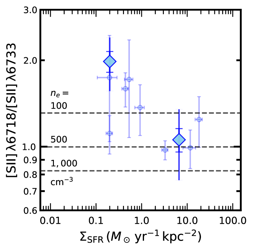
Figure 8.— Variation of $R(\text{{S~{}II}})$ with $\Sigma_{\rm SFR}$. Individual galaxies with detections of [S II] are indicated by the small symbols. The average $\langle\text{[{S~{}II}]}\rangle$ measured from the composite spectra are shown by the large diamonds. Capped vertical lines indicate measurement uncertainties, while uncapped vertical lines on the composite values include sample variance.

Figure 9.— Variation of O32 with $\Sigma_{\rm SFR}$. Individual galaxies with robust $\Sigma_{\rm SFR}$ measurements are indicated by the blue circles, and the large diamonds indicate the average values computed from composite spectra in two bins of O32. Capped vertical lines indicate measurement uncertainties, while uncapped vertical lines on the composite values include sample variance. In some cases, the error bars are smaller than the symbols. Also shown are measurements from the MOSDEF survey (small red circles), along with the best-fit relation to those data (red line). For comparison, the $z=9.51$ lensed galaxy from Williams et al. (2022) is indicated by the green star.

Table 3$\Sigma_{\rm SFR}$ Subsamples

$\Sigma_{\rm SFR}$ bin	$N_{\rm comp}$	$\langle z\rangle$	$\langle\Sigma_{\rm SFR}\rangle$	$\langle R(\text{{S~{}II}})\rangle$	$\langle{\rm O32}\rangle$
low	11	$3.570$	$0.20\pm 0.01$	$1.981\pm 0.165$ ($0.419$)	$1.899\pm 0.057$ ($0.314$)
high	11	$4.876$	$6.62\pm 0.27$	$1.057\pm 0.099$ ($0.293$)	$4.620\pm 0.107$ ($0.455$)

IV.4. Star-Formation-Rate Surface Density

The results of Section III imply a correlation between $n_{e}$ and $U$ (see also Shirazi et al. 2014; Bian et al. 2016; Papovich et al. 2022; Reddy et al. 2023b). In turn, we can explore the factors responsible for variations in $n_{e}$. Previous efforts have established a connection between $n_{e}$ and gas density, or SFR surface density (Shirazi et al., 2014; Shimakawa et al., 2015; Bian et al., 2016; Jiang et al., 2019; Davies et al., 2021; Reddy et al., 2023b). The JWST CEERS sample allows us to examine this connection at significantly higher redshifts ($z\gtrsim 2.7$) where galaxies may have a denser ISM on average. For this analysis, we considered the 22 galaxies in the sample that have existing measurements of effective half-light radii ($R_{\rm eff}$) from van der Wel et al. (2014). The SFR surface density is then defined as:

$$\Sigma_{\rm SFR}=\frac{\text{SFR(\text{H$\alpha$})}}{2\pi R_{\rm eff}^{2}},$$ (4)

and is expressed in units of $M_{\odot}$ yr^-1 kpc^-2. Similar to the analysis presented in Section III, the $\Sigma_{\rm SFR}$ subsample was divided into two equal-number bins of $\Sigma_{\rm SFR}$, and $\langle R(\text{{S~{}II}})\rangle$ and $\langle{\rm O32}\rangle$ were computed from the composite spectra constructed for galaxies in the two bins. The resulting values are listed in Table 3 and shown in Figures 8 and 9.

The difference in $\langle R(\text{{S~{}II}})\rangle$ between the low and high $\Sigma_{\rm SFR}$ bins is significant at the $\approx 4\sigma$ level, such that galaxies with higher $\Sigma_{\rm SFR}$ exhibit a lower $\langle R(\text{{S~{}II}})\rangle$ (or higher $\langle n_{e}\rangle\simeq 500$ cm^-3), similar to the trend suggested by earlier studies. As was the case for the relationship between $R(\text{{S~{}II}})$ and O32 (Figure 3), an accounting of sample variance indicates a large scatter in the relationship between $R(\text{{S~{}II}})$ and $\Sigma_{\rm SFR}$.

Of the correlations investigated in this analysis, the one between O32 and $\Sigma_{\rm SFR}$ appears to be the most significant (Figure 9): a Spearman correlation test indicates a $p$ value of $p=1.97\times 10^{-5}$. A similar and highly significant correlation was also found by Reddy et al. (2023b) for $z\sim 2-4$ galaxies in the MOSDEF survey. Data from that survey are also shown in Figure 9, along with the $z=9.51$ lensed galaxy from Williams et al. (2022), for comparison.

Figure 10 directly shows the relationship between $\log U$ inferred from photoionization modeling (Section IV.3.1) and $\Sigma_{\rm SFR}$ for the 22 galaxies with measurements of the latter. Again, a Spearman correlation test implies a highly significant correlation between $\log U$ and $\Sigma_{\rm SFR}$, with $p=3.2\times 10^{-4}$. A formal linear fit to the sample of 22 galaxies yields the following relation between $\log U$ and $\log[\Sigma_{\rm SFR}/M_{\odot}\,{\rm yr}^{-1}\,{\rm kpc}^{-2}]$:

$$\log U = (0.378\pm 0.021)\log\left[\frac{\Sigma_{\rm SFR}}{M_{\odot}\,{\rm yr}^{-1}\,{\rm kpc}^{-2}}\right]+$$ (5)

$$(-2.655\pm 0.011).$$

A similar fit to lower-redshift ($z\sim 1.9-3.7$) galaxies from the MOSDEF survey indicates a relation that is virtually identical to the one found here, despite the differences in the way the two samples were selected—i.e., rest-frame optical selection in the case of MOSDEF versus a heterogeneous selection in the case of CEERS. The starburst core of M82 (Förster Schreiber et al., 2001, 2003) is included in Figure 10, and is consistent with the trend between $U$ and $\Sigma_{\rm SFR}$ for the high-redshift samples. For context, the $z=9.51$ lensed galaxy in the RXJ2129 field reported by Williams et al. (2022) has $U=-1.24$ and an extremely high $\Sigma_{\rm SFR}\simeq 1000$ $M_{\odot}$ yr^-1 kpc^-2. These values place the $z\sim 9.5$ galaxy on the extrapolation of the $U$ vs. $\Sigma_{\rm SFR}$ relation established from the lower-redshift samples. This agreement, along with the virtually identical $U$ vs. $\Sigma_{\rm SFR}$ relations derived from the lower-redshift MOSDEF sample ($\langle z\rangle\simeq 2.1$) and the current sample ($\langle z\rangle\simeq 4.4$), may indicate that the $U$ vs. $\Sigma_{\rm SFR}$ relation does not evolve with redshift. If additional measurements for high-$\Sigma_{\rm SFR}$ galaxies confirm this lack of evolution, it would imply that the processes that couple $U$ to $\Sigma_{\rm SFR}$ are independent of redshift and that $\Sigma_{\rm SFR}$ is a key factor in modulating $U$ at any redshift.

Along these lines, we can examine whether $\Sigma_{\rm SFR}$ drives the variation in $U$ found for galaxies in our sample. Figure 11 displays the $\log U$ and $\log[Z_{\rm neb}/Z_{\odot}]$ values for the 22 galaxies with $\Sigma_{\rm SFR}$ measurements. It is clear that the scatter in $\log U$ at a given $\log[Z_{\rm neb}/Z_{\odot}]$ is related to $\Sigma_{\rm SFR}$. At a given $Z_{\rm neb}$, galaxies with the highest $U$ also have high $\Sigma_{\rm SFR}$.

Figure 10.— $\log U$ vs. $\Sigma_{\rm SFR}$ for the 22 galaxies in the sample with measurements of the latter. A Spearman test indicates a probability $p=3.2\times 10^{-4}$ that the correlation occurs by random chance, implying a highly significant correlation. A linear fit to the data indicates $\log U=(0.378\pm 0.021)\log[\Sigma_{\rm SFR}/M_{\odot}\,{\rm yr}^{-1}\,{\rm kpc}^{-2}]+(-2.655\pm 0.011)$ (blue line), with the $2\sigma$ confidence interval shown by the blue shaded region. The thick red line shows the best-fit correlation for $z=1.9-3.7$ galaxies in the MOSDEF survey (Reddy et al., 2023b), and is virtually identical to the relation for $z=2.7-6.3$ galaxies. The green star indicates the lensed $z=9.51$ galaxy from Williams et al. (2022). The purple diamond denotes the M82 starburst core studied in Förster Schreiber et al. (2001, 2003).

Figure 11.— $\log U$ vs. $\log[Z_{\rm neb}/Z_{\odot}]$ for the 22 galaxies in the sample with $\Sigma_{\rm SFR}$ measurements. The points are color coded by $\Sigma_{\rm SFR}$.

One result of our analysis is that $n_{e}$ appears to correlate with—but displays a large scatter with respect to—O32. There is also substantial scatter between $Q$ and O32 (Figure 3). On the other hand, we find highly significant correlations between O32 and $\Sigma_{\rm SFR}$, and between $\log U$ and $\Sigma_{\rm SFR}$. This raises the possibility that more than one of the parameters influencing $U$—namely $Q$, $n_{e}$, $\epsilon$, and $f_{\rm esc}$—is connected to $\Sigma_{\rm SFR}$. In other words, $\Sigma_{\rm SFR}$ may regulate more than one of the aforementioned parameters affecting $U$, causing $U$ to correlate tightly with $\Sigma_{\rm SFR}$. We now explore this possibility in the next few subsections.

IV.4.1 The Connection between $\Sigma_{\rm SFR}$ and $n_{e}$

We have already discussed the difference in $\langle n_{e}\rangle$ inferred for low- and high-$\Sigma_{\rm SFR}$ galaxies. A similar trend of increasing $n_{e}$ with $\Sigma_{\rm SFR}$ has been established in other low- and high-redshift samples, as noted above. The connection between $n_{e}$ and $\Sigma_{\rm SFR}$ may arise from the densities of molecular clouds that, at least initially, dictate densities in H II regions; the impact of stellar feedback on the densities and pressures in H II regions; and/or pressure equilibrium between H II regions and the ambient medium (e.g., Kaasinen et al. 2017; Davies et al. 2021).

IV.4.2 The Connection between $\Sigma_{\rm SFR}$ and $Q$

In parallel, several investigations have highlighted the link between SFR and $U$ (Nakajima & Ouchi, 2014; Kaasinen et al., 2018; Papovich et al., 2022; Reddy et al., 2023b) and its role in the redshift evolution of $U$ at a fixed stellar mass (e.g., Reddy et al. 2023b). Though we find no significant difference in the $\langle Q\rangle$ for the low- and high-O32 subsamples (Section III and Figure 3), an increase in SFR would imply a corresponding increase in $Q$, and hence $U$. The dynamic range of SFR probed in the current sample is not sufficient to readily observe an expected trend between SFR and $U$, highlighting the need to conduct a similar analysis on samples covering a larger dynamic range in SFR and other galaxy properties. Regardless, since the SFR is regulated by the gas supply and $Q\propto{\rm SFR}$, it follows that $Q$ must also be related to gas (or SFR) surface density.

IV.4.3 The Connection between $\Sigma_{\rm SFR}$ and $\epsilon$

Of the parameters that $U$ depends on, $\epsilon$ is the most difficult to constrain at high redshift as it requires calculating the volumes of line-emitting regions, which is beyond our capabilities given the limited spatial resolution of the current observations. Nevertheless, investigations of resolved local H II regions have established a well-known inverse correlation between $n_{e}$ and H II region size (Kim & Koo, 2001; Hunt & Hirashita, 2009). This “density-size” relation is typically attributed to the preferential location of compact H II regions in denser molecular clouds (Larson, 1981), and the density of such clouds is set by the gas or SFR surface density (e.g., Kennicutt & De Los Reyes 2021). Moreover, based on a sample of 58 H II regions in the disk of NGC 6946, Cedrés et al. (2013) find a significant anti-correlation between $\epsilon$ and H II region size. If these results are generalizable to other galaxies, they point to higher volume filling fractions in compact H II regions forming in dense-gas regions associated with high $\Sigma_{\rm SFR}$. A connection between $\epsilon$ and gas density is perhaps not surprising if density inhomogeneities are more pronounced in higher-density regions, leading to a larger filling fraction of dense clumps within H II regions. Consequently, $\epsilon$ may be connected to $\Sigma_{\rm SFR}$.

IV.4.4 The Connection between $\Sigma_{\rm SFR}$ and $f_{\rm esc}$

Finally, we noted in Section IV.2 that an increase in $f_{\rm esc}$ can lead to higher O32. Based on direct measurements locally (e.g., Gazagnes et al. 2018) and at $z\sim 2-3$ (Reddy et al., 2016; Steidel et al., 2018; Reddy et al., 2022), $f_{\rm esc}$ is tightly anti-correlated with the covering fraction of H I. The latter is likely regulated by stellar feedback and supernovae explosions that promote the formation of low column density or ionized channels in the ISM (e.g., Gnedin et al. 2008; Ma et al. 2016; Kimm et al. 2019; Ma et al. 2020; Cen 2020; Kakiichi & Gronke 2021). The volumetric impact of such feedback is enhanced in regions of high $\Sigma_{\rm SFR}$, particularly when coupled with a low gravitational potential as is the case for low-stellar-mass galaxies at high redshift (Reddy et al., 2022). Thus, a connection between $f_{\rm esc}$ and $\Sigma_{\rm SFR}$ would follow.

As discussed in Section IV.2, as $f_{\rm esc}$ increases, the dependence of $U$ on $n_{e}$ is expected to become weaker and eventually approach an inverse correlation. If this is the case, then significant outliers from the $U$ vs. $\Sigma_{\rm SFR}$ relation (Figure 10) may indicate objects where the positive scaling between $U$ and $n_{e}$ breaks down. This could occur if a significant fraction of $4\pi$ steradians is subtended by density-bounded regions (where $U$ would correlate negatively with $n_{e}$), or if the overlapping H II regions in the galaxy result in a more complicated scaling between $U$ and $n_{e}$. Further data are needed to test this potential avenue for identifying galaxies that may be leaking a substantial fraction of ionizing photons or that may otherwise have a complicated H II region geometry.

IV.4.5 Summary of $\Sigma_{\rm SFR}$ Considerations

The previous subsections point to the possibility that $\Sigma_{\rm SFR}$ affects essentially all of the parameters ($n_{e}$, $Q$, $\epsilon$, and $f_{\rm esc}$) that $U$ is sensitive to. Based on the previous discussion, all of these parameters may be expected to move in the same direction as $\Sigma_{\rm SFR}$, as long as $U$ positively correlates with $n_{e}$ (i.e., at low $f_{\rm esc}$). For increasing $f_{\rm esc}$—which would presumably indicate a high solid angle of density-bounded sightlines—the dependence of $U$ on $n_{e}$ should become noticeably weaker until an inverse correlation is established. In that case, the increase in apparent $U$ will be dominated by $f_{\rm esc}$ and $Q$. The aforementioned behaviors provide a natural explanation for why the scatter between any one of these parameters and $U$ may be large, while their combination, which is sensitive to $\Sigma_{\rm SFR}$, results in a highly significant correlation between $U$ and $\Sigma_{\rm SFR}$. This link between $U$ and $\Sigma_{\rm SFR}$ explains much of the scatter in $U$ at a fixed $Z_{\rm neb}$ (Figure 11)

Figure 12.— Variation of $R(\text{{S~{}II}})$ (top) and ${\rm O32}$ (bottom) with $M_{\ast}$. Individual galaxies with detections of [S II] and O32 measurements are indicated by small circles in the top and bottom panels, respectively. Mean measurements from composite spectra of galaxies are shown by the diamonds. Measurement uncertainties for individual and composite values are indicated by the capped vertical lines. Estimates of sample variance (including measurement error) for the composite values are indicated by the uncapped vertical lines. In some cases, the error bars are smaller than the symbols.

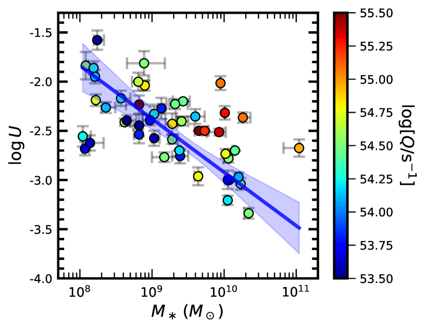
Figure 13.— Relationship between $U$ and $M_{\ast}$. Individual data points are color coded by $\log[Q/{\rm s}^{-1}]$. The best-fit linear relation between $\log U$ and $\log[M_{\ast}/M_{\odot}]$, and its $2\sigma$ confidence interval, are indicated by the solid blue line and shaded blue region, respectively. A formal fit gives $\log U=(-0.54+0.01)\log[M_{\ast}/M_{\odot}]+(2.51\pm 0.14)$.

Table 4$M_{\ast}$ Subsamples

$M_{\ast}$ bin	$N_{\rm comp}$	$\langle z\rangle$	$\langle M_{\ast}\rangle$	$\langle R(\text{{S~{}II}})\rangle$	$\langle{\rm O32}\rangle$
low	24	$4.766$	$8.60\pm 0.10$	$1.019\pm 0.184$ ($0.392$)	$4.847\pm 0.209$ ($1.270$)
high	24	$4.011$	$9.86\pm 0.10$	$1.704\pm 0.116$ ($0.306$)	$2.554\pm 0.078$ ($0.561$)

IV.5. Stellar Mass Considerations

Given the widespread use of stellar mass as a parameter in various galaxy scaling relations, such as the SFR vs. $M_{\ast}$ and mass-metallicity relations, it is useful to consider variations in $U$ and $n_{e}$ with $M_{\ast}$. The sample of 48 galaxies was divided into two bins of (low and high) $M_{\ast}$. Composite spectra were constructed for galaxies in each of the two bins, yielding the average measurements of $\langle R(\text{{S~{}II}})\rangle$ and $\langle{\rm O32}\rangle$ listed in Table 4 and displayed in Figure 12. The difference in $\langle R(\text{{S~{}II}})\rangle$ measured between the two mass bins is significant at the $3\sigma$ level, where galaxies with lower stellar masses exhibit an average [S II] ratio indicative of higher $\langle n_{e}\rangle\simeq 500$ cm^-3. This result contrasts with those of Shimakawa et al. (2015) and Sanders et al. (2016a) for somewhat lower-redshift galaxies ($z\sim 2.0-2.5$), where no significant correlation was found between $n_{e}$ and $M_{\ast}$. Along these lines, accounting for sample variance suggests a large scatter in $R(\text{{S~{}II}})$ at a given $M_{\ast}$. Indeed, Gburek et al. (2022) find an average $n_{e}$ consistent with the low-density limit ($\langle n_{e}\rangle\simeq 1$ cm^-3) for a sample of lensed star-forming galaxies at $z\sim 2.3$ with a median stellar mass of $\log[M_{\ast}/M_{\odot}]\simeq 8.3$. More precise estimates of $n_{e}$ for individual galaxies over a larger dynamic range in $M_{\ast}$ will be needed to further probe the relationship between $n_{e}$ and $M_{\ast}$.

Conversely, the relationship between ${\rm O32}$ and $M_{\ast}$ appears to be more significant as inferred from both the individual and composite measurements (see also Shapley et al. 2023a), consistent with observations at lower redshift (e.g., Sanders et al. 2016a). A Spearman test on the individual measurements indicates a probability $p=2.5\times 10^{-5}$ of a null correlation between O32 and $M_{\ast}$, while the difference in $\langle{\rm O32}\rangle$ between the low- and high-mass bins is significant at the $\simeq 10\sigma$ level. Folding in the effect of sample variance suggests a fairly large scatter in O32 at a given $M_{\ast}$, consistent with the spread of the individual O32 measurements at a given $M_{\ast}$.

Figure 13 displays the relation between $\log U$ and $M_{\ast}$ for the 48 galaxies in the sample. Not surprisingly, as with the relationship between O32 and $M_{\ast}$, a Spearman test indicates a probability $p=2.0\times 10^{-5}$ that the observed relation is drawn from an uncorrelated distribution of $\log U$ and $M_{\ast}$, implying a highly significant ($\gtrsim 4\sigma$) correlation. For reference, the best-fit linear correlation between $\log U$ and $\log[M_{\ast}/M_{\odot}]$ is indicated in the figure, along with the $2\sigma$ confidence interval on the fit. Given the higher $\Sigma_{\rm SFR}$ characteristic of low-mass galaxies (e.g., Shibuya et al. 2015), and the significant correlation between $\log U$ and $\Sigma_{\rm SFR}$ (see also Shimakawa et al. 2015; Reddy et al. 2023b), it is not surprising that an anti-correlation between $\log U$ and $M_{\ast}$ follows. It is worth noting, however, that the lower SFRs characteristic of low-mass galaxies implies a lower $Q$ (for a fixed $\xi_{\rm ion}$) and hence lower $U$ if all other parameters are kept fixed. Variations in $Q$ are likely responsible for some of the scatter seen in the relationship between $\log U$ and $\log[M_{\ast}/M_{\odot}]$. Specifically, Figure 13 shows that galaxies with the highest $Q$ in the sample generally lie above the mean relation between $\log U$ and $\log[M_{\ast}/M_{\odot}]$, while those with lower $Q$ generally lie below this relation. Thus the scatter in the relation between $\log U$ and $\log[M_{\ast}/M_{\odot}]$ is at least partly driven by variations in SFR.

Our analysis implies a strong anti-correlation between $\log U$ and $\log[M_{\ast}/M_{\odot}]$ for galaxies at $z=2.7-6.3$, similar to trends observed at lower redshifts. The strength of this anti-correlation and the apparently large scatter in the relationship between $n_{e}$ and $M_{\ast}$ suggests that other factors that influence $U$, namely $\epsilon$ and $f_{\rm esc}$, may also correlate inversely with $M_{\ast}$.

IV.6. What Drives the Relationship between $U$ and $Z_{\rm neb}$ at High Redshift?

We have argued that $\Sigma_{\rm SFR}$—which is tied to the gas surface density via the Kennicutt-Schmidt relation (Kennicutt, 1998; Kennicutt & De Los Reyes, 2021)—may play a central role in the variation in $U$ seen at high redshift. We should then address the source of the anti-correlation between $U$ and $Z_{\rm neb}$, at least when examined over a larger dynamic range in the latter. We suggest that this anti-correlation may stem from an increase in the average $\Sigma_{\rm SFR}$ with decreasing $Z_{\rm neb}$. While the data shown in Figure 11 do not support this hypothesis (i.e., there is a large spread in $\Sigma_{\rm SFR}$ at a fixed $Z_{\rm neb}$), enlarging the current sample and/or including other higher-redshift samples to probe the full range of $Z_{\rm neb}$ will be critical for determining how $Z_{\rm neb}$ depends on $\Sigma_{\rm SFR}$. The expectation of an inverse correlation between $\Sigma_{\rm SFR}$ and $Z_{\rm neb}$ appears to be borne out by spatially-resolved observations of local (Barrera-Ballesteros et al., 2018; Baker et al., 2023) and high-redshift galaxies (Troncoso et al., 2014), and would naturally follow from the anti-correlation between gas fraction and oxygen abundance (e.g., Barrera-Ballesteros et al. 2018; Sanders et al. 2023b). It is also worth noting that the lensed $z=9.51$ galaxy from Williams et al. (2022), one of the most metal-poor galaxies discovered to date with JWST, also has an extremely high $\Sigma_{\rm SFR}\simeq 1000$ $M_{\odot}$ yr^-1 kpc^-2.

The existence of an inverse correlation between $\Sigma_{\rm SFR}$ and $Z_{\rm neb}$, and a positive correlation between $U$ and $\Sigma_{\rm SFR}$ (Figure 10), then imply an inverse correlation between $U$ and $Z_{\rm neb}$. In this case, the high ionization parameters characteristic of galaxies with low oxygen abundances is tied to the fact that such galaxies also have high $\Sigma_{\rm SFR}$ on average (see also discussion in Reddy et al. 2023b). Future observations to constrain $U$, $Z_{\rm neb}$, and $\Sigma_{\rm SFR}$ or gas surface density in large samples of high-redshift galaxies will elucidate the relative roles of gas density and metallicity in shaping the distribution of $U$ found at high redshift.

V. Conclusions

We present the first statistical analysis of the connection between $U$, $n_{e}$, and $\Sigma_{\rm SFR}$ for $z=2.7-6.3$ star-forming galaxies. The sample consists of 48 galaxies with CEERS JWST/NIRSpec spectroscopy of rest-frame optical emission lines, 22 of which have robustly measured sizes and hence $\Sigma_{\rm SFR}$ measurements. Multiple Balmer emission lines were used to compute dust-corrected line fluxes and ratios, which were then fit with photoionization models to infer $U$ and $Z_{\rm neb}$. Our analysis indicates a correlation with a fairly large scatter between $n_{e}$ and O32, suggesting that gas density may play a role in driving the elevated $U$ observed for high-redshift galaxies. The ionizing photon rates, $Q$, appear to be uncorrelated with O32, likely owing to the limited dynamic range in SFR probed by the sample.

We discuss the role of metallicity in modulating $U$. No significant correlation is found between $U$ and $Z_{\rm neb}$ within the sample (e.g., see also Topping et al. 2020a), but this is likely due to the limited dynamic range in $Z_{\rm neb}$ probed by the current sample. The expected range of stellar metallicities for galaxies in the sample ($Z_{\ast}\lesssim 0.001$) implies that variations in the hardness or intensity of the ionizing spectrum are unlikely to be the main driver of $U$ in the sample. We consider the possibility that metallicity may affect $n_{e}$, and suggest that this is unlikely given the weakness of stellar winds—and thus the reduced impact they would have on the internal pressures and densities of H II regions—at low metallicity. We also consider the possibilities that dust diminishes and softens the ionizing spectrum with increasing $Z_{\rm neb}$, or that the stellar population synthesis models underpredict the increase in hardness or intensity of the ionizing spectrum with decreasing metallicity. However, these possibilities are not supported by the general agreement between ionization-rate-based and non-ionizing-photon-based SFRs for lower redshift ($z\sim 2-3$) galaxies, and the limited indirect constraints on the ionizing spectra of individual low-metallicity O stars (Telford et al., 2023).

The data imply that $n_{e}$ may correlate with $\Sigma_{\rm SFR}$, similar to findings from lower-redshift studies, though there is a large scatter in this correlation. On the other hand, we find a relatively tight and highly significant correlation between $U$ and $\Sigma_{\rm SFR}$, which appears to be redshift invariant at $z\sim 1.6-6.3$, and possibly up to $z\sim 9.5$. We point to the possibility that $\Sigma_{\rm SFR}$ may influence many (or all) of the factors that $U$ is sensitive to: $n_{e}$, $Q$, the volume filling factor $\epsilon$, and $f_{\rm esc}$. If all of these factors move in tandem with $\Sigma_{\rm SFR}$, as suggested by previous work, it would imply a highly significant correlation between $U$ and $\Sigma_{\rm SFR}$, consistent with our analysis. Finally, we confirm the existence of an anti-correlation between $U$ and $M_{\ast}$, similar to that established in lower-redshift ($z\lesssim 3$) galaxies. This anti-correlation would arise naturally from the higher $\Sigma_{\rm SFR}$ of low-mass galaxies (e.g., Shibuya et al. 2015). The main conclusion from this study is that the variation in $U$ within the sample of $z=2.7-6.3$ galaxies is not due to metallicity, but rather driven by $\Sigma_{\rm SFR}$, or more fundamentally, the gas surface density.

We suggest a number of followup investigations to improve on the existing analysis. Larger and more representative samples of high-redshift galaxies, covering larger dynamic ranges in properties such as SFR and O32, will be needed to further test the strength of the various correlations examined here. Deeper observations with higher $S/N$ spectra will enable the detection of weaker ionization- and abundance-sensitive lines, yielding tighter constraints on $U$ and, in particular, $Z_{\rm neb}$ using line ratios independent of those sensitive to $U$. Likewise, higher spectral resolution will be needed to resolve the [O II] $\lambda\lambda 3727,3730$ doublet, which is arguably a more useful probe of $n_{e}$ given its strength and slightly higher ionization potential relative to [S II]. Galaxy size measurements for larger samples will be crucial for constraining $\Sigma_{\rm SFR}$ and understanding the scatter between this property and $U$. Ultimately, direct measurements of gas surface densities (e.g., with ALMA) will be needed to more directly examine the link between gas density measured on kpc scales, and $n_{e}$ and $U$ which are sensitive to the ionized gas on H II-region scales. More extensive measurements of $n_{e}$ and $\epsilon$ in local H II regions (and simulations of the dynamical evolution of such regions), and how they relate to metallicity and SFR (or gas) surface density would benefit the interpretation of the relevant correlations (or lack thereof) seen at high redshift. These improvements will allow us to more rigorously quantify the role of metallicity and gas density in explaining the elevated $U$ inferred for high-redshift galaxies.

References

- Ali (2021) Ali, A. A. 2021, MNRAS, 501, 4136
- Baker et al. (2023) Baker, W. M., Maiolino, R., Belfiore, F., et al. 2023, MNRAS, 519, 1149
- Barrera-Ballesteros et al. (2018) Barrera-Ballesteros, J. K., Heckman, T., Sánchez, S. F., et al. 2018, ApJ, 852, 74
- Bian et al. (2016) Bian, F., Kewley, L. J., Dopita, M. A., & Juneau, S. 2016, ApJ, 822, 62
- Bouwens et al. (2016) Bouwens, R. J., Smit, R., Labbé, I., et al. 2016, ApJ, 831, 176
- Brinchmann et al. (2008) Brinchmann, J., Pettini, M., & Charlot, S. 2008, MNRAS, 385, 769
- Brott et al. (2011) Brott, I., de Mink, S. E., Cantiello, M., et al. 2011, A&A, 530, A115
- Buat et al. (2012) Buat, V., Noll, S., Burgarella, D., et al. 2012, A&A, 545, A141
- Bunker et al. (2023) Bunker, A. J., Saxena, A., Cameron, A. J., et al. 2023, arXiv e-prints, arXiv:2302.07256
- Calzetti et al. (2000) Calzetti, D., Armus, L., Bohlin, R. C., et al. 2000, ApJ, 533, 682
- Cardelli et al. (1989) Cardelli, J. A., Clayton, G. C., & Mathis, J. S. 1989, ApJ, 345, 245
- Cedrés et al. (2013) Cedrés, B., Beckman, J. E., Bongiovanni, Á., et al. 2013, ApJ, 765, L24
- Cen (2020) Cen, R. 2020, ApJ, 889, L22
- Chabrier (2003) Chabrier, G. 2003, PASP, 115, 763
- Conroy et al. (2009) Conroy, C., Gunn, J. E., & White, M. 2009, ApJ, 699, 486
- Cullen et al. (2019) Cullen, F., McLure, R. J., Dunlop, J. S., et al. 2019, MNRAS, 487, 2038
- Cullen et al. (2021) Cullen, F., Shapley, A. E., McLure, R. J., et al. 2021, MNRAS, 505, 903
- Daddi et al. (2007) Daddi, E., Dickinson, M., Morrison, G., et al. 2007, ApJ, 670, 156
- Davies et al. (2021) Davies, R. L., Schreiber, N. M. F., Genzel, R., et al. 2021, ApJ, 909, 78
- De Barros et al. (2016) De Barros, S., Reddy, N., & Shivaei, I. 2016, ApJ, 820, 96
- Dopita & Evans (1986) Dopita, M. A., & Evans, I. N. 1986, ApJ, 307, 431
- Dopita et al. (2006) Dopita, M. A., Fischera, J., Sutherland, R. S., et al. 2006, ApJ, 647, 244
- Draine (2011) Draine, B. T. 2011, ApJ, 732, 100
- Draine et al. (2007) Draine, B. T., Dale, D. A., Bendo, G., et al. 2007, ApJ, 663, 866
- Eldridge et al. (2017) Eldridge, J. J., Stanway, E. R., Xiao, L., et al. 2017, Publications of the Astronomical Society of Australia, 34, e058
- Ferland et al. (2017) Ferland, G. J., Chatzikos, M., Guzmán, F., et al. 2017, Revista Mexicana de Astronomia y Astrofisica, 53, 385
- Finkelstein et al. (2022) Finkelstein, S. L., Bagley, M. B., Ferguson, H. C., et al. 2022, arXiv e-prints, arXiv:2211.05792
- Förster Schreiber et al. (2001) Förster Schreiber, N. M., Genzel, R., Lutz, D., Kunze, D., & Sternberg, A. 2001, ApJ, 552, 544
- Förster Schreiber et al. (2003) Förster Schreiber, N. M., Genzel, R., Lutz, D., & Sternberg, A. 2003, ApJ, 599, 193
- Gazagnes et al. (2018) Gazagnes, S., Chisholm, J., Schaerer, D., et al. 2018, A&A, 616, A29
- Gburek et al. (2022) Gburek, T., Siana, B., Alavi, A., et al. 2022, arXiv e-prints, arXiv:2208.05976
- Giammanco et al. (2005) Giammanco, C., Beckman, J. E., & Cedrés, B. 2005, A&A, 438, 599
- Gnedin et al. (2008) Gnedin, N. Y., Kravtsov, A. V., & Chen, H.-W. 2008, ApJ, 672, 765
- Gordon et al. (2003) Gordon, K. D., Clayton, G. C., Misselt, K. A., Landolt, A. U., & Wolff, M. J. 2003, ApJ, 594, 279
- Groves et al. (2008) Groves, B., Dopita, M. A., Sutherland, R. S., et al. 2008, ApJS, 176, 438
- Hunt & Hirashita (2009) Hunt, L. K., & Hirashita, H. 2009, A&A, 507, 1327
- Inoue (2001) Inoue, A. K. 2001, AJ, 122, 1788
- Isobe et al. (2023) Isobe, Y., Ouchi, M., Nakajima, K., et al. 2023, arXiv e-prints, arXiv:2301.06811
- Jeong et al. (2020) Jeong, M.-S., Shapley, A. E., Sanders, R. L., et al. 2020, ApJ, 902, L16
- Jiang et al. (2019) Jiang, T., Malhotra, S., Yang, H., & Rhoads, J. E. 2019, ApJ, 872, 146
- Kaasinen et al. (2017) Kaasinen, M., Bian, F., Groves, B., Kewley, L. J., & Gupta, A. 2017, MNRAS, 465, 3220
- Kaasinen et al. (2018) Kaasinen, M., Kewley, L., Bian, F., et al. 2018, MNRAS, 477, 5568
- Kakiichi & Gronke (2021) Kakiichi, K., & Gronke, M. 2021, ApJ, 908, 30
- Kashino & Inoue (2019) Kashino, D., & Inoue, A. K. 2019, MNRAS, 486, 1053
- Kennicutt (1984) Kennicutt, R. C., J. 1984, ApJ, 287, 116
- Kennicutt & De Los Reyes (2021) Kennicutt, Robert C., J., & De Los Reyes, M. A. C. 2021, ApJ, 908, 61
- Kennicutt (1998) Kennicutt, R. C. 1998, ApJ, 498, 541
- Kim & Koo (2001) Kim, K.-T., & Koo, B.-C. 2001, ApJ, 549, 979
- Kimm et al. (2019) Kimm, T., Blaizot, J., Garel, T., et al. 2019, MNRAS, 486, 2215
- Kriek et al. (2009) Kriek, M., van Dokkum, P. G., Labbé, I., et al. 2009, ApJ, 700, 221
- Krumholz & Matzner (2009) Krumholz, M. R., & Matzner, C. D. 2009, ApJ, 703, 1352
- Kudritzki & Puls (2000) Kudritzki, R.-P., & Puls, J. 2000, ARA&A, 38, 613
- Langer (2012) Langer, N. 2012, ARA&A, 50, 107
- Larson (1981) Larson, R. B. 1981, MNRAS, 194, 809
- Leitherer et al. (2014) Leitherer, C., Ekström, S., Meynet, G., et al. 2014, ApJS, 212, 14
- Leitherer & Heckman (1995) Leitherer, C., & Heckman, T. M. 1995, ApJS, 96, 9
- Levesque & Richardson (2014) Levesque, E. M., & Richardson, M. L. A. 2014, ApJ, 780, 100
- Liu et al. (2008) Liu, X., Shapley, A. E., Coil, A. L., Brinchmann, J., & Ma, C.-P. 2008, ApJ, 678, 758
- Ma et al. (2016) Ma, X., Hopkins, P. F., Kasen, D., et al. 2016, MNRAS, 459, 3614
- Ma et al. (2020) Ma, X., Quataert, E., Wetzel, A., et al. 2020, MNRAS, 498, 2001
- Masters et al. (2016) Masters, D., Faisst, A., & Capak, P. 2016, ApJ, 828, 18
- Nagao et al. (2006) Nagao, T., Maiolino, R., & Marconi, A. 2006, A&A, 459, 85
- Naidu et al. (2022) Naidu, R. P., Matthee, J., Oesch, P. A., et al. 2022, MNRAS, 510, 4582
- Nakajima & Ouchi (2014) Nakajima, K., & Ouchi, M. 2014, MNRAS, 442, 900
- Nakajima et al. (2013) Nakajima, K., Ouchi, M., Shimasaku, K., et al. 2013, ApJ, 769, 3
- Nanayakkara et al. (2019) Nanayakkara, T., Brinchmann, J., Boogaard, L., et al. 2019, A&A, 624, A89
- Osterbrock & Flather (1959) Osterbrock, D., & Flather, E. 1959, ApJ, 129, 26
- Pacifici et al. (2015) Pacifici, C., da Cunha, E., Charlot, S., et al. 2015, MNRAS, 447, 786
- Pannella et al. (2015) Pannella, M., Elbaz, D., Daddi, E., et al. 2015, ApJ, 807, 141
- Papovich et al. (2011) Papovich, C., Finkelstein, S. L., Ferguson, H. C., Lotz, J. M., & Giavalisco, M. 2011, MNRAS, 412, 1123
- Papovich et al. (2022) Papovich, C., Simons, R. C., Estrada-Carpenter, V., et al. 2022, ApJ, 937, 22
- Pérez-Montero (2014) Pérez-Montero, E. 2014, MNRAS, 441, 2663
- Pérez-Montero et al. (2007) Pérez-Montero, E., Hägele, G. F., Contini, T., & Díaz, Á. I. 2007, MNRAS, 381, 125
- Reddy et al. (2010) Reddy, N. A., Erb, D. K., Pettini, M., Steidel, C. C., & Shapley, A. E. 2010, ApJ, 712, 1070
- Reddy et al. (2012) Reddy, N. A., Pettini, M., Steidel, C. C., et al. 2012, ApJ, 754, 25
- Reddy et al. (2006) Reddy, N. A., Steidel, C. C., Fadda, D., et al. 2006, ApJ, 644, 792
- Reddy et al. (2016) Reddy, N. A., Steidel, C. C., Pettini, M., Bogosavljević, M., & Shapley, A. E. 2016, ApJ, 828, 108
- Reddy et al. (2023a) Reddy, N. A., Topping, M. W., Sanders, R. L., Shapley, A. E., & Brammer, G. 2023a, arXiv e-prints, arXiv:2301.07249
- Reddy et al. (2018) Reddy, N. A., Oesch, P. A., Bouwens, R. J., et al. 2018, ApJ, 853, 56
- Reddy et al. (2020) Reddy, N. A., Shapley, A. E., Kriek, M., et al. 2020, ApJ, 902, 123
- Reddy et al. (2022) Reddy, N. A., Topping, M. W., Shapley, A. E., et al. 2022, ApJ, 926, 31
- Reddy et al. (2023b) Reddy, N. A., Sanders, R. L., Shapley, A. E., et al. 2023b, arXiv e-prints, arXiv:2302.10213
- Rémy-Ruyer et al. (2014) Rémy-Ruyer, A., Madden, S. C., Galliano, F., et al. 2014, A&A, 563, A31
- Robertson et al. (2013) Robertson, B. E., Furlanetto, S. R., Schneider, E., et al. 2013, ApJ, 768, 71
- Runco et al. (2021) Runco, J. N., Shapley, A. E., Sanders, R. L., et al. 2021, MNRAS, 502, 2600
- Sanders et al. (2023a) Sanders, R. L., Shapley, A. E., Topping, M. W., Reddy, N. A., & Brammer, G. B. 2023a, arXiv e-prints, arXiv:2301.06696
- Sanders et al. (2016a) Sanders, R. L., Shapley, A. E., Kriek, M., et al. 2016a, ApJ, 825, L23
- Sanders et al. (2016b) —. 2016b, ApJ, 816, 23
- Sanders et al. (2020) Sanders, R. L., Shapley, A. E., Reddy, N. A., et al. 2020, MNRAS, 491, 1427
- Sanders et al. (2023b) Sanders, R. L., Shapley, A. E., Jones, T., et al. 2023b, ApJ, 942, 24
- Schaerer et al. (2019) Schaerer, D., Fragos, T., & Izotov, Y. I. 2019, A&A, 622, L10
- Senchyna et al. (2017) Senchyna, P., Stark, D. P., Vidal-García, A., et al. 2017, MNRAS, 472, 2608
- Shapley et al. (2023a) Shapley, A. E., Reddy, N. A., Sanders, R. L., Topping, M. W., & Brammer, G. B. 2023a, arXiv e-prints, arXiv:2303.00410
- Shapley et al. (2023b) Shapley, A. E., Sanders, R. L., Reddy, N. A., Topping, M. W., & Brammer, G. B. 2023b, arXiv e-prints, arXiv:2301.03241
- Shibuya et al. (2015) Shibuya, T., Ouchi, M., & Harikane, Y. 2015, ApJS, 219, 15
- Shimakawa et al. (2015) Shimakawa, R., Kodama, T., Steidel, C. C., et al. 2015, MNRAS, 451, 1284
- Shirazi & Brinchmann (2012) Shirazi, M., & Brinchmann, J. 2012, MNRAS, 421, 1043
- Shirazi et al. (2014) Shirazi, M., Brinchmann, J., & Rahmati, A. 2014, ApJ, 787, 120
- Shivaei et al. (2015) Shivaei, I., Reddy, N. A., Steidel, C. C., & Shapley, A. E. 2015, ApJ, 804, 149
- Shivaei et al. (2016) Shivaei, I., Kriek, M., Reddy, N. A., et al. 2016, ApJ, 820, L23
- Shivaei et al. (2018) Shivaei, I., Reddy, N. A., Siana, B., et al. 2018, ApJ, 855, 42
- Shivaei et al. (2020) Shivaei, I., Reddy, N., Rieke, G., et al. 2020, ApJ, 899, 117
- Stanway & Eldridge (2018) Stanway, E. R., & Eldridge, J. J. 2018, MNRAS, 479, 75
- Stanway & Eldridge (2019) —. 2019, A&A, 621, A105
- Steidel et al. (2018) Steidel, C. C., Bogosavljević, M., Shapley, A. E., et al. 2018, ApJ, 869, 123
- Steidel et al. (2016) Steidel, C. C., Strom, A. L., Pettini, M., et al. 2016, ApJ, 826, 159
- Strom et al. (2018) Strom, A. L., Steidel, C. C., Rudie, G. C., Trainor, R. F., & Pettini, M. 2018, ApJ, 868, 117
- Strom et al. (2017) Strom, A. L., Steidel, C. C., Rudie, G. C., et al. 2017, ApJ, 836, 164
- Tang et al. (2023) Tang, M., Stark, D. P., Chen, Z., et al. 2023, arXiv e-prints, arXiv:2301.07072
- Telford et al. (2023) Telford, O. G., McQuinn, K. B. W., Chisholm, J., & Berg, D. A. 2023, ApJ, 943, 65
- Theios et al. (2019) Theios, R. L., Steidel, C. C., Strom, A. L., et al. 2019, ApJ, 871, 128
- Topping et al. (2020a) Topping, M. W., Shapley, A. E., Reddy, N. A., et al. 2020a, MNRAS, 499, 1652
- Topping et al. (2020b) —. 2020b, MNRAS, 495, 4430
- Trebitsch et al. (2017) Trebitsch, M., Blaizot, J., Rosdahl, J., Devriendt, J., & Slyz, A. 2017, MNRAS, 470, 224
- Troncoso et al. (2014) Troncoso, P., Maiolino, R., Sommariva, V., et al. 2014, A&A, 563, A58
- van der Wel et al. (2014) van der Wel, A., Chang, Y.-Y., Bell, E. F., et al. 2014, ApJ, 792, L6
- Vink (2022) Vink, J. S. 2022, ARA&A, 60, 203
- Vink et al. (2001) Vink, J. S., de Koter, A., & Lamers, H. J. G. L. M. 2001, A&A, 369, 574
- Williams et al. (2022) Williams, H., Kelly, P. L., Chen, W., et al. 2022, arXiv e-prints, arXiv:2210.15699
- Yeh & Matzner (2012) Yeh, S. C. C., & Matzner, C. D. 2012, ApJ, 757, 108