CAT-MOOD methods for conservation laws in one space dimension

Abstract

In this paper we blend high-order Compact Approximate Taylor (CAT) numerical methods with the a posteriori Multi-dimensional Optimal Order Detection (MOOD) paradigm to solve hyperbolic systems of conservation laws. The resulting methods are highly accurate for smooth solutions, essentially non-oscillatory for discontinuous ones, and almost fail-safe positivity preserving. Some numerical results for scalar conservation laws and systems are presented to show the appropriate behavior of CAT-MOOD methods.

0.1 Introduction

Lax-Wendroff methods for linear systems of conservation laws are based on Taylor expansions in time in which the time derivatives are transformed into spatial derivatives using the governing equations LeVeque2007book ; Toro2009 . The spatial derivatives are then discretised by means of centered high-order differentiation formulas.

black One of the difficulties to extend Lax-Wendroff methods to nonlinear problems come from the transformation of time derivatives into spatial derivatives through the Cauchy-Kovalesky (CK) procedure: this approach may indeed be impractical from the computational point of view. The Lax-Wendroff Approximate Taylor (LAT) methods introduced in ZBM2017 circumvent the CK procedure by computing time derivatives in a recursive way using high-order centered differentiation formulas combined with Taylor expansions in time. Compact Approximated Taylor methods (CAT) introduced in Carrillo-Pares follow a similar strategy. These methods are compact in the sense that the length of the stencils is minimal: $(2P+1)$-point stencils are used to get order $2P$ compared to $4P+1$-point stencils in LAT methods. They are also $L^{2}$ linearly-stable.

black A second difficulty comes from the treatment of shocks and discontinuities that usually arise in quasilinear systems of conservation laws. In order to avoid the spurious oscillations that Lax-Wendroff-type methods produce in presence of discontinuities or high gradients, CAT methods were combined in CPZMR2020 ; TesiPhD ; Macca-Pares with an a priori order adaptive procedure. black To do so a family of smoothness indicators were used to automatically reduce the order of the method black in the vicinity of discontinuities. black These limited CAT methods are called ACAT.

The goal of this paper is to combine black 1D CAT methods with the a posteriori Multi-dimensional Optimal Order Detection (MOOD) paradigm introduced in CDL1 ; CDL0_FVCA . black This technique is expected to produce non-oscillatory high-order methods with an appropriate detection of discontinuities The black resulting methods will be applied to scalar conservation laws and the 1D Euler equations of gas-dynamics.

The rest of this paper is organized as follows: the black next section introduces the system of equations we plan to solve. In section three, CAT methods are recalled. The fourth section describes how to blend CAT schemes with MOOD. black Numerical results are reported in the fifth section, illustrating the behavior of the sixth-order CAT-MOOD method. Conclusions and perspectives are finally drawn.

0.2 Governing equations

We consider 1D hyperbolic systems of conservation laws of the form

$$\partial_{t}\mathbf{U}+\partial_{x}\mathbf{F}(\mathbf{U})=\mathbf{0},$$ (1)

where $t\in\mathbb{R}^{+}$ represents the time variable, $x\in\mathbb{R}$ the space variable and $\mathbf{U}=\mathbf{U}(x,t)\in\mathbb{R}^{M}$ is the vector of conserved variables while $\mathbf{F}(\mathbf{U}(x,t))\in\mathbb{R}^{M}$ is the flux vector. More precisely, we focus on the 1D Euler equations of gas dynamics in which $M=3$, $\mathbf{U}=(\rho,\rho u,\rho e)^{t}$ with $\rho$ the density, $u$ the velocity and $e=\varepsilon+\frac{1}{2}{\color{black}u^{2}}$ the total energy black per unit mass, being $\varepsilon$ the specific black internal energy. The flux is given by $\mathbf{F}(\mathbf{U})=\left(\rho u,\rho u^{2}+p,(\rho e+p)u\right)^{t}$. The system is closed with the black perfect gas equation of state: ${\color{black}p(\rho,\varepsilon)=(\gamma-1)\rho\varepsilon}.$ The equations in (1) represent the conservation of mass, momentum and total energy. An entropy inequality has to be black supplemented to deal with discontinuous solutions. This system is hyperbolic with eigenvalues $\lambda^{-}=u-c$, $\lambda^{0}=u,$ $\lambda^{+}=u+c$ where $c=\sqrt{\gamma p/\rho}$ black is the sound speed. The set of admissible states, i.e. states that are consistent with physics, is

$$\mathcal{A}=\left\{\mathbf{U}\in\mathbb{R}^{M},\;\text{such that}\;\rho>0,\;p>0\right\}.$$ (2)

Together with this system, two scalar conservation laws black of the form

$$u_{t}+\partial_{x}f(u)=0,$$ (3)

will be considered to test the methods: black first the linear advection equation corresponding to $f(u)=bu$ with $b\in\mathbb{R}$, and, black secondly, Burgers’ equation corresponding to $f(u)=u^{2}/2$. black These scalar conservation laws verify the maximum principle, that is

$$\mathcal{A} = \left\{u\in\mathbb{R},\;\text{s.t.}\;\underline{u}_{0}\leq u(x,t)\leq\overline{u}_{0}\right\},$$

$$\underline{u}_{0} = \min_{x}(u(x,t_{0})),\;\overline{u}_{0}=\max_{x}(u(x,t_{0})),$$ (4)

where $t_{0}$ is the initial time, and $u(x,t_{0})$ the initial condition.

0.3 Compact Approximate Taylor (CAT) schemes

In this section we recall the formulation of CAT methods. In order to simplify the notation, the methods are introduced for scalar conservation laws (3), but the expression for systems (1) is similar.

We consider uniform meshes in 1D: the space domain is split into computational cells $\omega_{i}=[x_{i-1/2},x_{i+1/2}]$ of constant black width $\Delta x$. $x_{i}=\frac{1}{2}(x_{i+1/2}+x_{i-1/2})$ represents the center of the $i$-th cell. Although in practice the time step depends on the CFL condition and thus it is not constant, for the sake of simplicity in the presentation of the methods it will be assumed that the time interval $[0,T]$ is split into sub-intervals $[t^{n},t^{n+1}]$ of constant length $\Delta t$.

The $2P$-CAT method is written in conservative form as

$$u_{i}^{n+1}=u_{i}^{n}+\frac{\Delta t}{\Delta x}\left(F^{P}_{i-1/2}-F^{P}_{i+1/2}\right).$$ (5)

To compute the numerical flux $F^{P}_{i+1/2}$ only the approximations in the $2P$-point stencil

$$\mathcal{S}_{i+\frac{1}{2}}^{P}=\left\{x_{i-P+1},\ldots,x_{i+P}\right\}$$ (6)

are used, which ensures that $(2P+1)$ points are black employed to update the numerical solution. The following formulas of numerical differentiation are used to compute the numerical fluxes: given two positive integers $P$, $k$, an index $i$, and a real number $q$, we consider the interpolatory formula that approximates the $k$-th derivative of a function $f$ at the point $x_{i}+q\Delta x$ using its values at the $2P$ points $x_{i-P+1},\dots,x_{i+P}$:

$$f^{(k)}(x_{i}+q\Delta x)\approx\mathcal{A}^{k,j}_{P}(f,\Delta x)=\frac{1}{\Delta x^{k}}\sum_{j=-P+1}^{P}\gamma^{k,q}_{P,j}f(x_{i+j}).$$ (7)

black Notice that the case $k=0$ corresponds to Lagrange interpolation. When the formulas are applied to approximate the partial derivatives of a function $f(x,t)$ from some approximations $f_{i}^{n}\approx f(x_{i},t_{n})$, the symbol ${*}$ will be used to indicate to which variable (space or time) the differentiation is applied. For instance:

$$\partial^{k}_{x}f(x_{i},t_{n})\approx\mathcal{A}_{P}^{k,0}(f_{{*}}^{n},\Delta x\Bigr{)}=\frac{1}{\Delta x^{k}}\sum_{j=-P+1}^{P}\gamma^{k,0}_{P,l}f_{i+j}^{n},$$

$$\partial^{k}_{t}f(x_{i},t_{n})\approx\mathcal{A}_{P}^{k,0}(f_{i}^{{*}},\Delta t)=\frac{1}{\Delta t^{k}}\sum_{r=-P+1}^{P}\gamma^{k,0}_{P,r}f_{i}^{n+r}.$$

Using this notation, the expression of the numerical flux is as follows:

$$F^{P}_{i+1/2}=\sum_{k=1}^{m}\frac{\Delta t^{k-1}}{k!}\mathcal{A}^{0,1/2}_{P}(f_{i,{*}}^{(k-1)},\Delta x),$$ (8)

where

$$f^{(k-1)}_{i,j}\approx\partial_{t}^{k-1}f(u)(x_{i+j},t^{n}),\quad j=-P+1,\dots,P$$ (9)

are local approximations of the time derivatives of the flux. By local we mean that these approximations depend on the stencil, i.e. black for two different stencils such that $i_{1}+j_{1}=i_{2}+j_{2}$ then $f^{(k-1)}_{i_{1},j_{1}}$ is not necessarily equal to $f^{(k-1)}_{i_{2},j_{2}}$.

Since the exact solution satisfies

$$\partial_{t}^{k}u=-\partial_{t}^{k-1}f(u),$$

local approximations of the time derivatives of the solution are obtained black by :

$$u^{(k)}_{i,j}=-\mathcal{A}^{1,j}_{P}(f^{(k-1)}_{i,{*}},\Delta x)=-\frac{1}{\Delta x}\sum_{r=-P+1}^{P}\gamma^{1,j}_{P,r}f^{(k-1)}_{i,r}.$$

These approximations of the time derivatives are then adopted to compute black predicted values of the flux at several time levels, via recursive use of Taylor expansions, that will be then used to numerically approximate time derivatives of the flux at time level $n$. The algorithm to compute $F^{p}_{i+1/2}$ for the cell $i$ is then:

1. Define

   $$f^{(0)}_{i,j}=f(u^{n}_{i+j}),\quad j=-P+1,\dots,P.$$

2. For $k=2\dots m$:

   1. Compute

      $$u^{(k-1)}_{i,j}=-\mathcal{A}^{1,j}_{P}(f^{(k-2)}_{i,{*}},\Delta x).$$

   2. Compute

      $$f^{k-1,n+r}_{i,j}=f\left(u^{n}_{i+j}+\sum_{l=1}^{k-1}\frac{(r\Delta t)^{l}}{l!}u^{(l)}_{i,j}\right),\quad j,r=-P+1,\dots,P.$$

   3. Compute

      $$f^{(k-1)}_{i,j}=\mathcal{A}^{k-1,0}_{P}(f^{k-1,{*}}_{i,j},\Delta t),\quad j=-P+1,\dots,P.$$

3. Compute $F^{P}_{i+1/2}$ by

   $$F_{i+\frac{1}{2}}^{P}=\sum_{k=1}^{2P}\frac{\Delta t^{k-1}}{k!}f^{(k-1)}_{i+\frac{1}{2}},$$ (10)

   where

   $$f^{(k-1)}_{i+\frac{1}{2}}=\mathcal{A}_{P}^{0,\frac{1}{2}}\left(f^{(k-1)}_{i,*},\Delta x\right),\quad\text{with}\quad\mathcal{A}_{P}^{0,\frac{1}{2}}\left(f^{(k-1)}_{i,*},\Delta x\right)=\sum_{p=-P+1}^{P}\gamma_{P,p}^{0,\frac{1}{2}}\,f_{i+p}^{(k-1)}.$$

0.4 CATMOOD

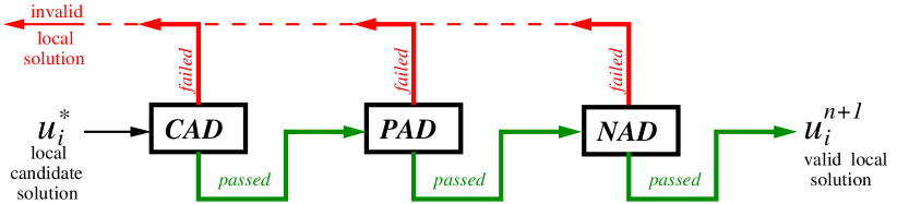
The essential idea of the MOOD technique is to apply a high-order method over the entire domain for a time step, then check locally, for each cell $i$, the behavior of the solution using some admissibility criteria such as positivity, monotonicity, physical black admissibility, etc. If the solution computed in cell $i$ at time $t^{n+1}$ is in accordance with the selected criteria, it is kept. Otherwise it is black locally recomputed with a lower order numerical method. This operation is repeated until acceptability, or when a robust first order scheme is black employed.

Bearing this in mind, the idea is to design a cascade of CAT methods in which the order is locally adjusted according to some a posteriori admissibility criteria thus creating a new family of adaptive CAT methods called CAT-MOOD schemes.

0.4.1 MOOD admissibility criteria

Following CDL2 ; CDL3 , we select three different admissibility criteria which are used to check the admissibility of a candidate numerical solution $\left\{u_{i}^{n+1}\right\}_{1\leq i\leq N}$:

1. Physical Admissible Detector (PAD): The first detector checks the physical validity of the candidate solution. In particular, this detector reacts to negative solution when a variable cannot take negative values: this is the case of the pressure $p$ and density $\rho$ for the 1D Euler system in compliance with (2).

2. Numerical Admissible Detector (NAD): This criterion is used to ensure the essentially non-oscillatory (ENO) character of the numerical solution, namely that no large and spurious minima or maxima are introduced locally in the solution. To do this, the following relaxed variant of the Discrete Maximum Principle (see Ciarlet ; CDL1 ) is black considered:

   $$\min_{j\in\mathcal{C}_{i}^{P}}(u_{j}^{n})-\delta_{i}^{n}\leq u_{i}^{n+1}\leq\max_{j\in\mathcal{C}_{i}^{P}}(u^{n}_{j})+\delta_{i}^{n},$$

   where $\mathcal{C}_{i}^{P}=\{i-P,\ldots,i+P\}$ is the $(2P+1)$-point centered stencil and $\delta_{i}$ is a parameter that avoids wrong detections in flat region. Here, $\delta_{i}$ is set as:

   $$\delta_{i}^{n}=\max\left({\color{black}{\rm tol}_{1}},{\color{black}{\rm tol}_{2}},\max_{j\in\mathcal{C}_{i}^{P}}u^{n}_{j}-\min_{j\in\mathcal{C}_{i}^{P}}u^{n}_{j}\right).$$ (11)

   In the Euler test of Sec. 0.5 the relaxed discrete maximum principle is only computed for density $\rho$ and pressure $p$.

3. Computer Admissible Detector (CAD): The last criterion detects undefined or unrepresentable quantities, usually not-a-number NaN or infinity quantity black which may appear, for instance, when a division by zero black is encountered.

The order in which these three criteria are applied to the candidate solution is showed in Figure 1-left. If one of the criteria is not satisfied, the cell is marked black as ’failed’. A new candidate solution is then computed in marked cells using a lower order method and it is checked again.

(a) Criteria

(b) Cascade

Figure 1: Left: Detection criteria of the MOOD technique for a candidate solution $u_{i}^{*}$. Computer Admissible Detector (CAD), Physical Admissible Detector (PAD) and Numerical Admissible Detector (PAD) — Right: Order cascades of CAT schemes used in the MOOD procedure. Starting from the most accurate one, CAT6, downgrading to lower order schemes, and, at last to a $1$st order accurate scheme employed to ensure robustness.

0.4.2 CAT scheme with MOOD limiting

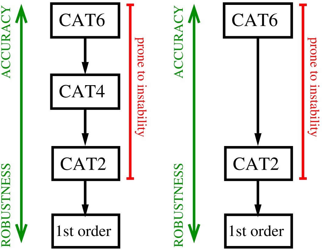
In this work, CAT methods are used as high-order methods within the MOOD strategy: the natural idea would be, black given a target order $2P$, to use the black following cascade of numerical methods

$$\text{CAT}2P\to\text{CAT}2(P-1)\to\dots\text{CAT}2\to\text{First-order method}$$

to obtain a method with order of accuracy $2P$ in smooth regions and an essentially non-oscillatory solution close to discontinuities or large gradients. black However, in order to reduce the computational cost, the following cascade has been black preferred in the numerical tests below

$$\text{CAT}6\to\text{CAT}2\to\text{First-order method}$$

where the first-order method is Rusanov for scalar problems and HLL for Euler equations: see Figure 1-right black for an illustration. Therefore, the expected order of accuracy in smooth regions is 6. The resulting scheme is referred to as CATMOOD6.

0.5 Numerical test cases

black Three tests are considered, namely linear advection equation, to check the numerical order of accuracy, Burgers equation, and Euler equations of gas dynamics, to check shock-capturing capability of the method. In all our tests we used the following parameters: ${\rm tol}_{1}=10^{-4}$ and ${\rm tol}_{2}=10^{-3}$.

0.5.1 Scalar linear equation with smooth initial condition

Let us consider the linear conservation law (3) with black $f(u)=u$, and periodic boundary conditions in $[0,2\pi]$. The smooth initial condition is given by

$$u(x,0)=u_{0}(x)=\frac{1}{2}\sin(x)+1.$$ (12)

The goal of this test is to check and compare the empirical order of accuracy of CATMOOD6. For smooth solutions, the detectors are expected not to spoil the sixth-order of accuracy of the CAT6 black scheme. We run this test case in the interval $[0,2\pi],$ with final time $t_{fin}=1$, CFL$=0.9,$ and periodic boundary conditions. We apply CAT6 and CATMOOD6 method on successive refined uniform meshes going from $10$ to $320$ cells. As expected the empirical order of accuracy of both CAT and CATMOOD is 6: see Table 1. black We observe that below $N=80$ cells, the mesh is not fine enough to allow for a clean limiting. black Notice that this threshold depends on the parameteters ${\rm tol}_{1}$ and ${\rm tol}_{2}$ adopted in (11). Larger values of these parameter will lower the threshold to smaller values of $N$. Moreover, in this test, CATMOOD6 is $1.5$ more expensive than CAT6.

Linear equation - Error, Rate of convergence, CPU time
	CAT6			CATMOOD6
$N$	$L^{1}$ error	order	CPU time	$L^{1}$ error	order	CPU time
10	4.27$\times 10^{-5}$	—	0.0073	8.34$\times 10^{-3}$	—	0.016
20	6.93$\times 10^{-7}$	5.95	0.020	3.18$\times 10^{-3}$	1.39	0.031
40	9.64$\times 10^{-9}$	6.17	0.038	3.16$\times 10^{-4}$	3.33	0.053
80	1.43$\times 10^{-10}$	6.07	0.068	2.48$\times 10^{-6}$	3.67	0.094
160	2.09$\times 10^{-12}$	6.09	0.13	2.09$\times 10^{-12}$	23.50	0.2
320	3.29$\times 10^{-14}$	5.99	0.25	3.31$\times 10^{-14}$	5.99	0.38
	Expected	6		Expected	6

Table 1: Linear scalar equation 0.5.1. $L^{1}-$norm errors between the numerical solution and the exact solution of the linear equation at $t_{\text{final}}=1$ on uniform Cartesian mesh and CFL$=0.9.$

0.5.2 Burgers’ equation with non-smooth initial condition

Let us consider (3) with black $f(u)=u^{2}/2$, periodic boundary conditions, and non-smooth initial condition

$$u_{0}(x)=\begin{cases}1.1\quad\;\;\;\mathrm{if}\quad 0\leq x\leq\frac{1}{2};\\ 2.1\quad\;\;\;\mathrm{if}\quad\frac{1}{2}<x<\frac{3}{2};\\ 0.1\quad\;\;\;\mathrm{if}\quad\frac{3}{2}\leq x\leq\frac{17}{10}.\end{cases}$$ (13)

We run this test case with first-order Rusanov-flux and CATMOOD6 method in the interval $[0,1.7],$ with final time $t_{fin}=0.65$, using a 50-cell mesh, CFL$=0.9,$ and periodic boundary conditions. Figure 2 shows the initial condition and the numerical solutions obtained with both methods: it can be seen that CATMOOD6 provides a non-oscillatory solution black still providing better resolution than the first order method. Notice that larger values of the thresholds tol₁ and tol₂ will decrease dissipation, but may not be sufficient to avoid creation of spurious oscillations.

(a) Numerical solutions at time $t=0.3$.

(b) Numerical solutions at time $t=0.65$.

Figure 2: Burgers’ equation with non-smooth initial condition 0.5.2 — Left: Numerical solutions at time $t=0.3$ — Right: Numerical solutions at final time $t_{fin}=0.65$ obtained with Rusanov flux and CATMOOD6 on $50$ uniform mesh and CFL$=0.9$. Rusanov flux scheme has been used as first order. The reference solution has been obtained with the 1st order Rusanov scheme on $2000$ uniform cells.

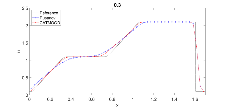
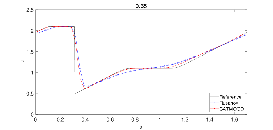
0.5.3 Euler system: Sod problem

Let us consider Euler equations (3) with SOD initial condition

$$(\rho,{\color{black}u},p)=\left\{\begin{array}[]{ll}\displaystyle(1,0,1)&\mbox{if }x\leq 0,\\ \displaystyle(0.125,0,0.1)&\mbox{if }x>0.\end{array}\right.$$ (14)

(a) Density.

(b) Zoom of the density on shock

(c) Velocity.

(d) Pressure

Figure 3: Euler system: Sod problem 0.5.3 — Left-up: Numerical solutions for density $\rho$ at final time $t=0.3$ obtained with black 1st order HLL flux and CATMOOD6, on $200$ uniform mesh and CFL$=0.9$. — Right-up: Zoom of the numerical solutions and reference one. — Left/right-down: same as left-up but for velocity and pressure variables. The reference solution is the exact one.

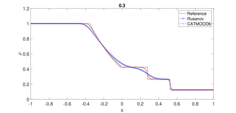
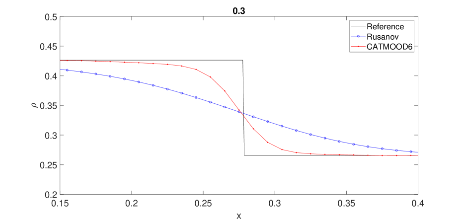
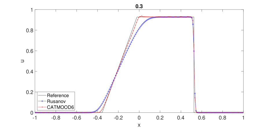
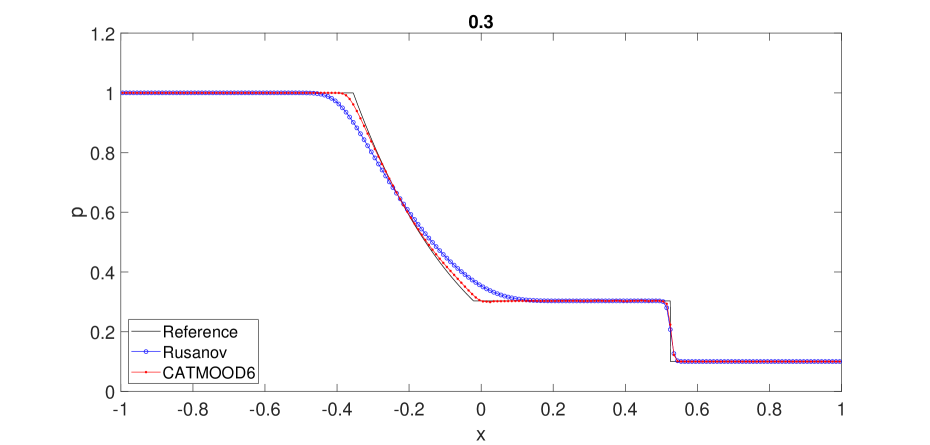
We run this test case with first-order Rusanov-flux and CATMOOD6 method in the interval $[-1,1],$ with final time $t_{fin}=0.3$. We use a $200-$cell mesh, CFL$=0.9,$ and free boundary conditions. Figure 3 shows the numerical and the exact solutions for density, velocity and pressure obtained with both methods and a zoom of the density close to the shock. It can be seen that, as expected, CATMOOD6 solution shows a better resolution of rarefaction and contact waves.

0.6 Conclusion and perspectives

In this paper we have presented a combination between the a posteriori shock-capturing MOOD technique and the one-step high-order finite-difference CAT2P schemes. CAT2P schemes are of order $2P$ on smooth solutions, but, black an extra dissipative mechanism must be supplemented to deal with steep gradients or discontinuous solutions. In this work we rely on an a posteriori MOOD paradigm which computes an unlimited high-order candidate solution at time $t^{n+1}$, and, further detects troubled cells which are recomputed with a lower-order scheme throughout a family of detectors. For a proof of concept, we tested the so-called black CATMOOD6 scheme based on the ’cascade’: CAT6$\rightarrow$CAT2$\rightarrow\,$ 1st, where the last scheme is a first order robust scheme. black This scheme has been challenged on a test suite of smooth solutions (linear scalar equation), simple shock waves (Burgers’ equation), and complex self-similar solutions involving contact, shock and rarefaction waves (Sod problem). In all test cases, CATMOOD6 has preserved the accuracy on smooth parts of the solutions, an essentially-non-oscillatory behavior close to steep gradients, and, black always produces a physically valid solution. black A detailed analysis of the improvement in the efficiency over standard slope limiters has not been performed. A two dimensional implementation, as well as other generalizations and improvements are under way.

References

- [1] H. Carrillo, E. Macca, C. Parés, G. Russo, and D. Zorío. An order-adaptive compact approximate taylor method for systems of conservation law. Journal of Computational Physics, 438:31, 2021.
- [2] H. Carrillo and C. Parés. Compact approximate taylor methods for systems of conservation laws. J. Sci. Comput., 80:1832–1866, 2019.
- [3] P.G. Ciarlet. Discrete maximum principle for finite-difference operators. Aeq. Math., 4:338–352, 1970.
- [4] S. Clain, S. Diot, and R. Loubère. A high-order finite volume method for systems of conservation laws – multi-dimensional optimal order detection (MOOD). J. Comput. Phys., 230(10):4028 – 4050, 2011.
- [5] S. Clain, S. Diot, and R. Loubère. Multi-dimensional optimal order detection (mood) — a very high-order finite volume scheme for conservation laws on unstructured meshes. In Fort Fürst Halama Herbin Hubert (Eds.), editor, FVCA 6, International Symposium, Prague, June 6-10, volume 4 of Series: Springer Proceedings in Mathematics, 2011. 1st Edition. XVII, 1065 p. 106 illus. in color.
- [6] S. Diot, S. Clain, and R. Loubère. Improved detection criteria for the multi-dimensional optimal order detection (MOOD) on unstructured meshes with very high-order polynomials. Computers and Fluids, 64:43 – 63, 2012.
- [7] S. Diot, R. Loubère, and S. Clain. The MOOD method in the three-dimensional case: Very-high-order finite volume method for hyperbolic systems. International Journal of Numerical Methods in Fluids, 73:362–392, 2013.
- [8] R.J. LeVeque. Finite difference methods for ordinary and partial differential equations: steady-state and time-dependent problems (Classics in Applied Mathematics). Society for Industrial and Applied Mathematics, Philadelpia, PA. USA., 1 edition, 2007.
- [9] E. Macca. Shock-Capturing methods: Well-Balanced Approximate Taylor and Semi-Implicit schemes. PhD thesis, Università degli Studi di Palermo, Palermo, 2022.
- [10] E. Macca, H. Carrillo, C. Parés, and G. Russo. Well-Balanced Adaptive Compact Approximate Taylor methods for systems of balance laws. Journal of Computational Physics, 478, 2023.
- [11] E.F. Toro. Riemann Solvers and Numerical Methods for Fluid Dynamics. Springer, third edition, 2009.
- [12] D. Zorío, A. Baeza, and P. Mulet. An approximate Lax-Wendroff-type procedure for high order accurate scheme for hyperbolic conservation laws. J. Sci. Comput., 71(1):246–273, 2017.