An Effective Multivariate Normality Test via Hessians of Empirical Cumulant Generating Functions

Abstract

In this article, we propose a new class of consistent tests for $p$-variate normality. These tests are based on the characterization of the standard multivariate normal distribution, that the Hessian of the corresponding cumulant generating function is identical to the $p\times p$ identity matrix and the idea of decomposing the information from the joint distribution into the dependence copula and all marginal distributions. Under the null hypothesis of multivariate normality, our proposed test statistic is independent of the unknown mean vector and covariance matrix so that the distribution-free critical value of the test can be obtained by Monte Carlo simulation. We also derive the asymptotic null distribution of proposed test statistic and establish the consistency of the test against different fixed alternatives. Last but not least, a comprehensive and extensive Monte Carlo study also illustrates that our test is a superb yet computationally convenient competitor to many well-known existing test statistics.

Keywords: moment generating function; consistency; goodness-of-fit test; $L^{2}$-statistic; empirical cumulant generating function

1 Introduction

The normal distribution is certainly one of the most important distributions in statistics that underlie many statistical procedures. Therefore, validation of the normality assumption behind the data is of fundamental importance and interest; to this end, there are a significant number of tests for both univariate and multivariate normality in the literature. For instance, Mecklin and Mundfrom (2004) surveyed dozens of common multivariate normality tests and divided most of the tests into four categories: (i) procedures based on graphical plots and correlation coefficients; (ii) goodness-of-fit tests; (iii) test based on measures of skewness and kurtosis; (iv) and tests based on the empirical characteristic functions. Furthermore, there is still an ongoing research devoted in developing new normality tests. For example, Ebner and Henze (2020) reviewed the recent developments in tests for multivariate normality with an emphasis on asymptotic properties of several classes of weighted $L^{2}$-statistics, where these statistics are mostly based on empirical moment generating functions or empirical characteristic functions.

In this article, we introduce a novel test for multivariate normality based on a system of second order partial derivatives of the cumulant generating function and decomposing a joint distribution into the dependence copula and all marginal distributions. Let $X$ be a random vector on $\mathbb{R}^{p}$. Denote $\mathcal{N}_{p}$ to be the class of all non-degenerate $p$-variate normal distributions. Suppose that we observe a random sample of $X_{1},\ldots,X_{n}$ having the same joint distribution as that of $X$. We consider the traditional and conventional problem of testing the null hypothesis:

$$H_{0}:\text{The law of $X$ belongs to }\mathcal{N}_{p},$$

against the general alternative hypothesis:

$$H_{1}:\text{The law of $X$ does not belong to }\mathcal{N}_{p}.$$

Let $\overline{X}_{n}:=n^{-1}\sum^{n}_{i=1}X_{i}$ be the sample mean and $S_{n}:=n^{-1}\sum^{n}_{i=1}(X_{i}-\overline{X}_{n})(X_{i}-\overline{X}_{n})^{\top}$ be the (biased) sample covariance matrix. Let $S^{-1/2}_{n}$ denote the unique symmetric square root of $S^{-1}_{n}$. For the rest of this article, we assume that $n\geq p+1$. Due to the absolute continuity of the multivariate normal distribution, $S^{-1}_{n}$ exists with probability one under $H_{0}$, see for example Eaton and Perlman (1973). Therefore, under the alternative hypothesis, if $S_{n}$ is not invertible, we can simply reject the null hypothesis. Thus, from now on we assume $S^{-1}_{n}$ exists. It is known that, under the null hypothesis, the distribution of the so-called scaled residuals $Z_{n,i}:=S^{-1/2}_{n}(X_{i}-\overline{X}_{n})$, $i=1,\ldots,n$, does not depend on the mean vector $\mu$ and covariance matrix $\Sigma$ of $X$; also see Szkutnik (2021) for details. In other words, the distribution of the scaled residuals when $X$ is from any non-degenerate multivariate normal distribution is the same as that when $X\sim N_{p}(0,\textbf{I}_{p})$. Thus, for test statistics that only involve the scaled residuals $Z_{n,i}$’s, under the null hypothesis, it suffices to consider the case $X\sim N_{p}(0,\textbf{I}_{p})$, where $\textbf{I}_{p}$ denotes the $p\times p$ identity matrix. Denote $M(t):=\mathbb{E}(e^{t^{\top}X})$ to be the moment generating function of $X$. The cumulant generating function of $X$ is also defined by $\Lambda(t):=\log M(t)$, for $t$ in the proximity of origin. Our proposed test relies on the following key observation: if $X\sim N_{p}(0,\textbf{I}_{p})$, then

$$H_{\Lambda}(t)=\textbf{I}_{p},\quad t\in\mathbb{R}^{p},$$ (1)

where $H_{f}$ denotes the Hessian matrix of a function $f$; clearly, the converse is also true, namely if the Hessian of the cumulant generating function of a random vector is identically equal to $\textbf{I}_{p}$, then the random vector has a standard multivariate normal distribution.

In general, a random vector can deviate from the multivariate normality from two causes: (i) at least one marginal distribution of a component random variable is non-normal; or (ii) the copula structure of the random vector is not the Gaussian one; see for example Nelsen (2006). In fact, practitioners often look at univariate normal Q-Q plots, P-P plots (Gan and Koehler (1990)) and bivariate plots of the marginals taken any two at a time, by performing univariate tests on each of the marginal distribution as well as performing tests based on dimension reduction (e.g., a test of the squared radii $Z_{n,i}^{T}Z_{n,i}$’s); see Chapter 9 in Thode (2002). These create multiple testing issues, and using Bonferroni rule to combine them as an adjustment can be conservative. Motivated by the fact that a multivariate distribution can be determined by specifying its corresponding marginal distributions and dependence structure, for any $t=(t_{1},\ldots,t_{p})^{\top}\in\mathbb{R}^{p}$, define the function $M^{*}(\cdot)$ via the decomposition

$$M(t)\equiv\left(\prod^{p}_{j=1}M_{j}(t_{j})\right)M^{*}(t),$$

where $M_{j}(\cdot)$ is the moment generating function of the $j$th component of $X$. Further, if $M$ is twice differentiable, then

$$H_{\log M^{*}}(t)\equiv H_{\log M}(t)-\sum^{p}_{j=1}H_{\log M_{j}}(t_{j}).$$ (2)

Denote $\Lambda_{j}:=\log M_{j}$ and $\Lambda^{*}:=\log M^{*}$. We rewrite (2) as

$$H_{\Lambda^{*}}(t)\equiv H_{\Lambda}(t)-D(t),$$ (3)

where $D(t)$ is a $p\times p$ diagonal matrix with elements $H_{\Lambda_{1}}(t_{1}),\ldots,H_{\Lambda_{p}}(t_{p})$ in order. Under the null hypothesis $H_{0}$, by (1),

$$H_{\Lambda^{*}}(t)=\textbf{0}_{p\times p}\text{ and }D(t)=\textbf{I}_{p},\text{ for all }t\in\mathbb{R}^{p},$$ (4)

where $\textbf{0}_{p\times p}$ is the $p\times p$ zero matrix. Our proposed test is based on an empirical version of the two identities of (4).

Recall that under $H_{0}$, the scaled residuals $Z_{n,i}$’s are independent of the unknown $\mu$ and $\Sigma$, and they will resemble a random sample from $N_{p}(0,\textbf{I}_{p})$. Let $M^{(n)}(t):=\frac{1}{n}\sum^{n}_{i=1}e^{t^{\top}Z_{n,i}}$, $\triangledown M^{(n)}(t):=\frac{1}{n}\sum^{n}_{i=1}Z_{i}e^{t^{\top}Z_{n,i}}$ and $H_{M^{(n)}}(t):=\frac{1}{n}\sum^{n}_{i=1}Z_{n,i}Z_{n,i}^{\top}e^{t^{\top}Z_{n,i}}$ be the empirical version of the unknown theoretical moment generating function, its gradient and Hessian based on the scaled residuals, respectively. An empirical version $H_{\Lambda^{(n)}}$ of $H_{\Lambda}$ using the scaled residuals is then given by

$$H_{\Lambda^{(n)}}(t):=\frac{M^{(n)}(t)H_{M^{(n)}}(t)-\triangledown M^{(n)}(t)(\triangledown M^{(n)}(t))^{\top}}{M^{(n)}(t)^{2}},$$ (5)

where $\Lambda^{(n)}:=\log M^{(n)}$. The corresponding empirical version of $H_{\Lambda^{*}_{n}}$ is

$$H_{(\Lambda^{(n)})^{*}}(t)=H_{\Lambda^{(n)}}(t)-D^{(n)}(t),$$

where $D^{(n)}(t)$ is the $p\times p$ diagonal matrix with elements $H_{\Lambda^{(n)},11}(s_{1}),\ldots,H_{\Lambda^{(n)},pp}(s_{p})$. Here, $s_{j}=(0,\ldots,0,t_{j},0,\ldots,0)^{\top}$, where $t_{j}$ is in the $j$th position of this $p$-vector. In view of (4), a large value of the $L^{2}$-statistics $n\int\cdots\int_{\mathbb{R}^{p}}\sum_{i=1}^{p}\sum^{p}_{j>i}H^{2}_{(\Lambda^{(n)})^{*},ij}(t)dt$ or $n\int\cdots\int_{\mathbb{R}^{p}}\sum^{p}_{i=1}(D^{(n)}_{ii}(t)-1)^{2}dt$ is an evidence against $H_{0}$. Since these two integrals do not generally admit a closed form expression because of the denominator $M^{(n)}(t)$ in (5), we consider their discretized approximations and define the following statistics:

$$H^{(n)}_{N}=n\sum^{N}_{l=1}\sum^{p}_{i=1}\sum^{p}_{j>i}H^{2}_{(\Lambda^{(n)})^{*},ij}(t_{l})\quad\text{ and }\quad D^{(n)}_{N}=n\sum^{N}_{l=1}\sum^{p}_{i=1}(D^{(n)}_{ii}(t_{l})-1)^{2},$$ (6)

where $\{t_{1},\ldots,t_{N}\}$ is a collection of vectors in $\mathbb{R}^{p}$. For example, we may choose them randomly in the ball $\{t\in\mathbb{R}^{p}:\|t\|\leq R\}$ for some $R>0$ and $\|\cdot\|$ is the usual Euclidean norm. Our simulation studies show that $R=3$ will work well in most scenarios. To see why a moderate value (like $3$) can be a good choice, we can write (5) as

$$H_{\Lambda^{(n)}}(t)=\sum^{n}_{i=1}Z_{n,i}Z_{n,i}^{\top}W_{n,i}(t)-\left(\sum^{n}_{i=1}Z_{n,i}W_{n,i}\right)\left(\sum^{n}_{i=1}Z_{n,i}W_{n,i}\right)^{\top},$$ (7)

where $W_{n,i}(t):=\frac{e^{t^{\top}Z_{n,i}}}{\sum^{n}_{j=1}e^{t^{\top}Z_{n,j}}}$ and $H_{\Lambda^{(n)}}(t)$ can be interpreted as a weighted estimate of the covariance matrix. Under $H_{0}$, $Z_{n,i}$ behaves like a random vector from $N(0,\textbf{I}_{p})$ under $H_{0}$ so that all the components of $Z_{n,i}$ will be around $-3$ to $3$ most of the time. A larger value of $\|t\|$ tend to put more weights to extreme values of $Z_{n,i}$’s in (7). Thus, a moderate value of $R$ can avoid $H^{(n)}_{N}$ and $D^{(n)}_{N}$ depend heavily on only a few extreme values of $Z_{n,i}$’s. On the other hand, if $R$ is small, then the weights are more even and less information in the empirical cumulant generating function is used, which may result in a less powerful test (recall that the population version identities in (4) hold for all values of $t\in\mathbb{R}^{p}$ under $H_{0}$).

We can interpret $H^{(n)}_{N}$ as capturing the overall deviation from multivariate normality dependence structure while $D^{(n)}_{N}$ focuses on the deviation from marginal univariate normality. Note that $D^{(n)}_{N}$ is still a function of the scaled residuals, so that it does not depend on the mean and covariance matrix of the normal distribution under $H_{0}$. The computation of $H^{(n)}_{N}$ and $D^{(n)}_{N}$ is straightforward as we essentially only have to compute the scaled residuals and the empirical Hessian of the cumulant generating function given in (5) at different values of $t$. Since the magnitudes of $H^{(n)}_{N}$ and $D^{(n)}_{N}$ are different, to combine evaluative assessment $H^{(n)}_{N}$ and $D^{(n)}_{N}$, we define our proposed test statistic to be

$$T^{(n)}_{N}=\max\bigg{\{}\frac{H^{(n)}_{N}-\mathbb{E}^{S}(H^{(n)}_{N})}{SD^{S}(H^{(n)}_{N})},\frac{D^{(n)}_{N}-\mathbb{E}^{S}(D^{(n)}_{N})}{SD^{S}(D^{(n)}_{N})}\bigg{\}},$$ (8)

such that we reject $H_{0}$ for large values of $T^{(n)}_{N}$. Here, the superscript “$S$” refers to the calculations based on $S$ simulations: $\mathbb{E}^{S}(H^{(n)}_{N}):=\frac{1}{S}\sum^{S}_{s=1}H^{(n)}_{N,s}$, $SD^{S}(H^{(n)}_{N}):=\sqrt{\frac{1}{S-1}(\sum^{S}_{s=1}H^{(n)}_{N,s}-\mathbb{E}^{S}(H^{(n)}_{N}))^{2}}$, and $H^{(n)}_{N,s}$ is computed as in $H^{(n)}_{N}$ but using the scaled residuals from the $s$-th random sample of $X_{1,s},\ldots,X_{n,s}\stackrel{{\scriptstyle i.i.d.}}{{\sim}}N(0,\textbf{I}_{p})$; that is, $\mathbb{E}^{S}(H^{(n)}_{N})$ and $SD^{S}(H^{(n)}_{N})$ are the estimated mean and standard deviation of $H^{(n)}_{N}$ from $S$ independent Monte Carlo simulations. Similar definitions and interpretation apply to $\mathbb{E}^{S}(D^{(n)}_{N})$ and $SD^{S}(D^{(n)}_{N})$. Since we shall find the critical values of the test statistic using simulation, these estimates can be obtained as a byproduct at the same time.

For testing univariate normality, we base on the fact that $\Lambda^{\prime\prime}(t)=1$ for all $t\in\mathbb{R}$ if $X\sim N(0,1)$, and define its empirical and discrete approximate:

$$U^{(n)}_{N}:=\sum^{N}_{l=1}((\Lambda^{(n)})^{\prime\prime}(t_{l})-1)^{2},$$ (9)

where for some $t_{1},\ldots,t_{N}\in\mathbb{R}$,

$$(\Lambda^{(n)})^{\prime\prime}(t):=\frac{M^{(n)}(t)(M^{(n)})^{\prime\prime}(t)-(M^{(n)})^{\prime}(t))^{2}}{(M^{(n)})^{2}(t)},$$

such that we reject $H_{0}$ for large values of $U^{(n)}_{N}$. Under the null hypothesis, $T^{(n)}_{N}$ is independent of the unknown mean vector $\mu$ and covariance matrix $\Sigma$ for the multivariate case, and $U^{(n)}_{N}$ is independent of the unknown mean and variance for the univariate case. In Section 3, we shall further show that our test is consistent especially when the moment generating function exists and is twice differentiable. In general, one cannot find a test that is uniformly powerful than all the other tests against all alternatives. In Section 4, through an extensive simulation study, we see that our proposed test often has higher powers over various alternative distributions compared with some prevalent common tests as well as some recently formulated tests. In particular, for the univariate case, our test performs the best in various short-tailed symmetric and asymmetric distributions compared with other common normality test, including the well-known and powerful Shapiro-Wilk test (Shapiro and Wilk (1965)). For the multivariate case, our proposed test outperforms other common tests in many of the short-tailed distributions and some of the long-tailed distributions. For other distributions, the proposed test tends to have powers in between those of different tests.

The organization of the paper is as follows. In Section 2, we derive the asymptotic distribution of the test statistic $T^{(n)}_{N}$ under the null hypothesis $H_{0}$. Consistency of the newly proposed test statistic will be established in Section 3. We provide a comprehensive Monte Carlo simulation study in Section 4. Discussion and conclusion are given in Section 5. Technical proofs and additional simulation results are appended in the section of supplementary materials.

2 Asymptotic Null Distribution

In this section, we derive the asymptotic distribution of the test statistic $T^{(n)}_{N}$ under the null hypothesis that each sample $X_{i}$ has a nondegenerate multivariate normal distribution. Recall that our proposed test statistic is independent of the mean and covariance matrix of $X$. To derive the asymptotic null distribution, it therefore suffices to consider the case when $\mathbb{E}(X)=0$ and $Var(X)=\textbf{I}_{p}$.

Let $M^{(n)}_{0}(t):=\frac{1}{n}\sum^{n}_{i=1}e^{t^{\top}X_{i}}$, $\triangledown M^{(n)}_{0}(t):=\frac{1}{n}\sum^{n}_{i=1}X_{i}e^{t^{\top}X_{i}}$ and $H_{M^{(n)}_{0}}(t):=\frac{1}{n}\sum^{n}_{i=1}X_{i}X_{i}^{\top}e^{t^{\top}X_{i}}$ be the empirical moment generating function, its gradient and Hessian based on $X_{i}$’s (not the scaled residuals $Z_{n,i}$’s), respectively. The corresponding population versions are $M_{0}(t)=e^{\|t\|^{2}/2}$, $\triangledown M_{0}(t)=e^{\|t\|^{2}/2}t$ and $H_{M_{0}}(t)=e^{\|t\|^{2}/2}(tt^{\top}+\textbf{I}_{p})$. Define $f_{0}:\mathbb{R}^{p}\times\mathbb{R}^{p}\rightarrow\mathbb{R}$, $f_{1}:\mathbb{R}^{p}\times\mathbb{R}^{p}\rightarrow\mathbb{R}^{p}$ and $f_{2}:\mathbb{R}^{p}\times\mathbb{R}^{p}\rightarrow\mathbb{R}^{p\times p}$ one by one as follows:

$$f_{0}(x;t) :=e^{\|t\|^{2}/2}\left\{-t^{\top}x-\frac{(t^{\top}x)^{2}}{2}+\frac{\|t\|^{2}}{2}\right\};$$

$$f_{1}(x;t) :=e^{\|t\|^{2}/2}\left\{-(\textbf{I}_{p}+tt^{\top})x-\frac{1}{2}(2\textbf{I}_{p}+tt^{\top})(xx^{\top}-\textbf{I}_{p})t\right\};$$

$$f_{2}(x;t) :=e^{\|t\|^{2}/2}\bigg{\{}-\frac{1}{2}(xx^{\top}-\textbf{I}_{p})(\textbf{I}_{p}+tt^{\top})-xt^{\top}-\frac{1}{2}(\textbf{I}_{p}+tt^{\top})(xx^{\top}-\textbf{I}_{p})-tx^{\top}$$

$$\quad-\frac{1}{2}\sum^{p}_{h=1}\sum^{p}_{k=1}\left(\frac{\partial tt^{\top}}{\partial t_{h}}+tt^{\top}t_{h}+t_{h}\textbf{I}_{p}\right)t_{k}(x_{h}x_{k}-\mathbbm{1}(h=k))-(\textbf{I}_{p}+tt^{\top})t^{\top}x\bigg{\}},$$

where $\mathbbm{1}(\cdot)$ is the indicator function. Since $\mathbb{E}(X)=0,\mathbb{E}(XX^{\top})=\textbf{I}_{p}$ and $\mathbb{E}((t^{\top}X)^{2})=t^{\top}\mathbb{E}(XX^{\top})t=\|t\|^{2}$, straightforward calculation shows that $\mathbb{E}(f_{j}(X_{i};t))=0$ for $j=0,1,2$ and any $t\in\mathbb{R}^{p}$, where the same notation $0$ is adopted as the zero element in the corresponding high dimensional space if there is no cause of ambiguity. Also, let $Q^{h}:=\frac{\partial tt^{\top}}{\partial t_{h}}$. $Q^{h}$ is a matrix of $0$’s except for the $h$th row and $h$th column, where the $(h,j)$ element, $Q^{h}_{hj}=t_{j}$ for $j=1,\ldots,h-1,h+1,\ldots,p$; while the $(i,h)$ element, $Q^{h}_{ih}=t_{i}$ for $i=1,\ldots,h-1,h+1,\ldots,p$, and $Q^{h}_{hh}=2t_{h}$. The following lemma first gives the approximation errors due to the use of scaled residuals in the empirical version of the moment generating function and its gradient and Hessian.

Lemma 1.

Under $H_{0}$, for any $t\in\mathbb{R}^{p}$, we have

1. $M^{(n)}(t)-M^{(n)}_{0}(t)=n^{-1}\sum^{n}_{i=1}f_{0}(X_{i};t)+o_{p}(n^{-1/2})$;

2. $\triangledown M^{(n)}(t)-\triangledown M^{(n)}_{0}(t)=n^{-1}\sum^{n}_{i=1}f_{1}(X_{i};t)+o_{p}(n^{-1/2})$;

3. $H_{M^{(n)}}(t)-H_{M^{(n)}_{0}}(t)=n^{-1}\sum^{n}_{i=1}f_{2}(X_{i};t)+o_{p}(n^{-1/2})$.

Define $g_{1},g_{2}:\mathbb{R}^{p}\times\mathbb{R}^{p}\rightarrow\mathbb{R}^{p\times p}$ by

$$g_{1}(x;t) :=e^{\|t\|^{2}/2}\left\{e^{t^{\top}x}(xx^{\top}+tt^{\top}-tx^{\top}-xt^{\top}-\textbf{I}_{p})\right\},$$

$$g_{2}(x;t) :=e^{\|t\|^{2}/2}\left\{f_{2}(x;t)+(tt^{\top}+\textbf{I}_{p})f_{0}(x;t)-tf^{\top}_{1}(x;t)-f_{1}(x;t)t^{\top}-2f_{0}(x;t)\textbf{I}_{p}\right\}.$$

As $\mathbb{E}(e^{t^{\top}X}XX^{\top})=e^{\|t\|/2}(tt^{\top}+\textbf{I}_{p})$ and $\mathbb{E}(e^{t^{\top}X}X)=te^{\|t\|^{2}/2}$, we have $\mathbb{E}(g_{1}(X_{i};t))=0$. Also, $\mathbb{E}(g_{2}(X_{i};t))=0$ because $\mathbb{E}(f_{j}(X_{i};t))=0$ for $j=0,1,2$. To derive the asymptotic distribution of the test statistic $T^{(n)}_{N}$, we first derive that of $\sqrt{n}(H_{\Lambda^{(n)}}(t)-\textbf{I}_{p})$. Since

$$H_{\Lambda^{(n)}}(t)-\textbf{I}_{p}=(M^{(n)})^{-2}(t)\cdot\{M^{(n)}(t)H_{M^{(n)}}(t)-\triangledown M^{(n)}(t)(\triangledown M^{(n)}(t))^{\top}-(M^{(n)})^{2}(t)\textbf{I}_{p}\},$$

we establish the following lemma, which write the second term of the right side of the above equation into an average of mean zero terms of independent variable and asymptotic negligible reminder.

Lemma 2.

Under $H_{0}$, for any $t\in\mathbb{R}^{p}$, we have

1. $M^{(n)}_{0}(t)H_{M^{(n)}_{0}}(t)-\triangledown M^{(n)}_{0}(t)(\triangledown M^{(n)}_{0}(t))^{\top}-(M^{(n)}_{0})^{2}(t)\textbf{I}_{p}=n^{-1}\sum^{n}_{i=1}g_{1}(X_{i};t)+o_{p}(n^{-1/2})$;

2. $M^{(n)}(t)H_{M^{(n)}}(t)-\triangledown M^{(n)}(t)(\triangledown M^{(n)}(t))^{\top}-(M^{(n)})^{2}(t)\textbf{I}_{p}=n^{-1}\sum^{n}_{i=1}(g_{1}(X_{i};t)+g_{2}(X_{i};t))+o_{p}(n^{-1/2})$.

With Lemmas 1 and 2, we have the following theorem.

Theorem 1.

Under $H_{0}$, for any $t\in\mathbb{R}^{p}$, we have

$$\sqrt{n}(H_{\Lambda^{(n)}}(t)-\textbf{I}_{p})=\frac{1}{\sqrt{n}}\sum^{n}_{i=1}h(X_{i};t)+o_{p}(1),$$

where $h(x;t):=e^{-\|t\|}(g_{1}(x;t)+g_{2}(x;t))$.

Consider $t_{1},\ldots,t_{N}\in\mathbb{R}^{p}$ in (6). For a $p\times p$ matrix $A=(a_{ij})$, we denote $A^{v}=(a_{11},\ldots,a_{1p},a_{22},\ldots,a_{2p},\ldots,a_{pp})$ to be the vectorization of the upper triangular part of $A$. By Theorem 1, the multivariate central limit theorem and Slutsky’s theorem, we have

$$(\sqrt{n}(H^{v}_{\Lambda^{(n)}}(t_{1})-\textbf{I}^{v}_{p}),\ldots,\sqrt{n}(H^{v}_{\Lambda^{(n)}}(t_{N})-\textbf{I}^{v}_{p}))^{\top}\stackrel{{\scriptstyle d}}{{\rightarrow}}N_{p(p+1)N/2}(0,\Sigma_{N}),$$

where the $(i,j)$-th element of $\Sigma_{N}$ is $\text{Cov}(h^{v}_{i^{\prime}}(X;t_{l}),h^{v}_{j^{\prime}}(X;t_{l^{\prime}}))$, for $i=(l-1)p(p+1)/2+i^{\prime},j=(l^{\prime}-1)p(p+1)/2+j^{\prime},l,l^{\prime}=1,\ldots,N,i^{\prime},j^{\prime}=1,\ldots,p(p+1)/2$. By the continuous mapping theorem, we can immediately obtain the limiting distributions of $H^{(n)}_{N}$, $D^{(n)}_{N}$, and $T^{(n)}_{N}$ respectively of, denoted by, $H_{N},D_{N}$ and $T_{N}$, where

$$T_{N}:=\max\left\{\frac{H_{N}-\mathbb{E}^{S}(H_{N})}{SD^{S}(H_{N})},\frac{D_{N}-\mathbb{E}^{S}(D_{N})}{SD^{S}(D_{N})}\right\},$$

with $\mathbb{E}^{S}(H_{N}):=\frac{1}{S}\sum^{S}_{s=1}H_{N,s}$, $SD^{S}(H_{N}):=\sqrt{\frac{1}{S-1}\sum^{S}_{s=1}(H_{N,s}-\mathbb{E}^{S}(H_{N}))}$, and $H_{N,1},\ldots,H_{N,S}$ is a random sample having the same distribution as $H_{N}$. Similar definition applies to $\mathbb{E}^{S}(D_{N})$ and $SD^{S}(D_{N})$. We do not try to simplify the asymptotic null distribution $T_{N}$ further because the critical value of the test statistic at any finite sample size can be approximated by simulation.

3 Consistency

While the scaled residuals $Z_{n,i}$ of a multivariate normal with a general covariance matrix are equal in distribution as the scaled residuals of a standard multivariate normal distribution, such a nice property does not hold with $X$ is in the alternative hypothesis. To study the convergence of $H_{N}^{(n)}$ and $D_{N}^{(n)}$ for a general $X$ with finite second moments, we can assume $E(X)=0$ without loss of generality, and $Var(X)=\Sigma$. Denote $\tilde{X}:=\Sigma^{-1/2}X$, $\tilde{M}(t)=\mathbb{E}(e^{t^{\top}\tilde{X}})$ and $\tilde{\Lambda}(t):=\log\tilde{M}(t)$. The following theorem establishes the strong limits of $U^{(n)}_{N}$ for the univariate case, and that of $H^{(n)}_{N}$ and $D^{(n)}_{N}$ for the multivariate case, altogether imply the consistency of our test.

Theorem 2.

Suppose that the moment generating function of $X$ exists and is twice differentiable.

1. If $X$ is univariate, with probability $1$,

   $$\lim_{n\rightarrow\infty}\frac{U^{(n)}_{N}}{n}=\sum^{N}_{l=1}(\tilde{\Lambda}^{\prime\prime}(t_{l})-1)^{2}.$$

2. If $X$ is multivariate, with probability $1$,

   $$\lim_{n\rightarrow\infty}\frac{H^{(n)}_{N}}{n} =\sum^{N}_{l=1}\sum^{p}_{i=1}\sum^{p}_{j>i}(H_{\tilde{\Lambda}^{*},ij}(t_{l}))^{2},$$

   $$\lim_{n\rightarrow\infty}\frac{D^{(n)}_{N}}{n} =\sum^{N}_{l=1}\sum^{p}_{i=1}(\tilde{D}_{ii}(t_{li})-1)^{2},$$

   where $H_{\tilde{\Lambda}^{*}}$ and $\tilde{D}_{ii}$ are defined similarly as in (3).

Suppose that the moment generating function of $X$ exists and is twice differentiable but $X$ is not from $\mathcal{N}_{p}$. Then, $\tilde{X}$ is not distributed as $N_{p}(0,\textbf{I}_{p})$ and there must exist a point $t^{*}$ in the neighbourhood of $0$ such that $H_{\tilde{\Lambda}}(t^{*})\neq\textbf{I}_{p}$. Since $H_{\tilde{\Lambda}}(\cdot)$ is continuous, there exists a neighbourhood $\mathcal{O}$ of $t^{*}$ such that $H_{\tilde{\Lambda}}(t)\neq\textbf{I}_{p}$ for all $t\in\mathcal{O}$. This implies that $H_{\tilde{\Lambda}^{*}}(t)\neq 0$ or $\tilde{D}(t)\neq\textbf{I}_{p}$ for all $t\in\mathcal{O}$. As a result, if $\{t_{l}\}^{N}_{l=1}$ is chosen using a space-filling design and $N$ is large enough, some $t_{l}$ will be in $\mathcal{O}$. Hence, almost surely, $\lim_{n\rightarrow\infty}H^{(n)}_{N}=\infty$ or $\lim_{n\rightarrow\infty}D^{(n)}_{N}=\infty$ so that $\lim_{n\rightarrow\infty}T^{(n)}_{N}=\infty$. In practice, one can also perform the test with a large enough $N$ and see if the $p$-value is stable when $N$ increases.

4 Simulation Studies

We carried out extensive Monte Carlo study to evaluate the finite-sample sizes and powers of our proposed test statistics and compare with several tests in the literature. For the univariate case, we compare with

1. the Cramér-von Mises (CvM) test (Cramér (1928), Mises (1931), and Smirnov (1936));

2. the Anderson-Darling (AD) test (Anderson and Darling (1954));

3. the Shapiro-Wilk (SW) test (Shapiro and Wilk (1965));

4. the Jarque-Bera (JB) test (Jarque and Bera (1987));

5. the Henze-Visagie (HV) test (Henze and Visagie (2020)).

The first four tests are well-known and will not be reviewed; see Yap and Sim (2011) for a review of these tests. For the implementation of CvM and AD, the functions cvm.test and ad.test in the R package nortest are used, respectively. The SW test can be carried out using Shapiro.test in the stats R package. The JB test is carried out using jarque.bera.test from the R package tseries. The HV test is developed based on a system of first-order partial differential equations that characterize the moment generating function of the $p$-variate standard normal distribution. The test statistic is

$$HV_{n,\gamma}:=n\int_{\mathbb{R}^{p}}\|\triangledown M^{(n)}(t)-tM^{(n)}(t)\|^{2}\exp(-\gamma\|t\|^{2})dt,$$ (10)

which can be computed in a closed-form formula; see equation (9) in (Henze and Visagie (2020)). $H_{0}$ is rejected for large values of $HV_{n,\gamma}$. Henze and Visagie (2020) recommended $\gamma=5$ to be used when performing the test based on their numerical results and we follow this suggestion in our numerical study. The R package mnt contains the function HV to compute this test statistic. For our proposed test statistic and the HV test statistic, $100,000$ independent replications were used to determine the critical value of the tests. Each size or power estimate is based on $10,000$ replications. We largely follow the choices of alternative distributions considered in Yap and Sim (2011), where various shapes of distributions were considered. The alternative distributions considered here can be classified into symmetric short-tailed distributions, symmetric long-tailed distributions, asymmetric distributions, and mixture of normal distributions.

We first define additional notation for some of these distributions. Denote GLD$(\lambda_{1},\lambda_{2},\lambda_{3},\lambda_{4})$ to be the genearlized lambda distribution proposed by Ramberg and Schmeiser (1974), which is a four-parameter generalization of the two-parameter Tukey’s Lambda family of distribution (Hastings Jr et al. (1947)). The percentile function of GLD$(\lambda_{1},\lambda_{2},\lambda_{3},\lambda_{4})$ is given as

$$Q(y)=\lambda_{1}+\frac{y^{\lambda_{3}}-(1-y)^{\lambda_{4}}}{\lambda_{2}},\quad\text{where }0\leq y\leq 1,$$

where $\lambda_{1}$ is the location parameter, $\lambda_{2}$ is the scale parameter and $\lambda_{3}$ and $\lambda_{4}$ are the shape parameters. The density function of GLD$(\lambda_{1},\lambda_{2},\lambda_{3},\lambda_{4})$ at $x=Q(y)$ is

$$f(x)=\frac{\lambda_{2}}{\lambda_{3}y^{\lambda_{3}-1}-\lambda_{4}(1-y)^{\lambda_{4}-1}}.$$

The truncated normal distribution of a normal distribution with mean $\mu$ and standard deviation $\sigma$ truncated to the interval $(a,b)$ is denoted by Trunc$(a,b,\mu,\sigma)$. The scale-contaminated normal distribution, denote by ScConN$(p,b)$, is a mixture of two normal distributions with probability $p$ from a normal distribution $N(0,b^{2})$ and probability $1-p$ from $N(0,1)$. LoConN$(p,a)$ denotes the distribution of a mixture of two normal distributions with probability $p$ from a normal distribution with mean $a$ and variance $1$ and with probability $1-p$ from a standard normal distribution.

The symmetric short-tailed distributions include $U(0,1)$, Beta$(0.5,0.5)$, Beta$(2,2)$, $\allowbreak\text{GLD}(0,1,0.25,0.25)$, GLD$(0,1,0.5,0.5)$, GLD$(0,1,0.75,0.75)$, GLD$(0,1,1.25,1.25)$, $\allowbreak\text{Trunc}(-2,2,0,1)$, $\allowbreak\text{Trunc}(-3,3,0,2)$, and $\text{Trunc}(-2,2,0,2)$. The symmetric long-tailed distributions include Laplace, logistic, GLD$(0,1,-0.1,-0.1)$, GLD$(0,1,-0.15,-0.15)$, $t(5)$, $t(10)$, and $t(15)$. The asymmetric distributions include exp$(1)$, lognormal$(0,0.5)$, Gamma$(4,5)$, Beta$(2,1)$, Beta$(3,2)$, Weibull$(3,1)$, Pareto$(1,3)$, $\chi^{2}(4)$, $\chi^{2}(10)$, and $\chi^{2}(20)$. The normal mixtures considered are ScConN$(0.2,5)$, ScConN$(0.05,5)$, LoConN$(0.5,3)$, and LoConN$(0.5,2)$.

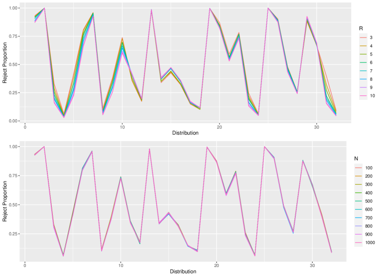
Figure 1: Univariate test under alternatives when $n=50$. The upper panel shows the empirical reject proportions under the $32$ alternative distributions when $N=500$ with different values of $R$. The lower panel shows the empirical reject proportions under the $32$ alternative distributions when $R=3$ with different values of $N$.

In the simulation study, the set of points $\{t_{1},\ldots,t_{N}\}$ is chosen randomly from $\{t\in\mathbb{R}^{p}:\|t\|\leq R\}$. The upper panel of Figure 1 shows the empirical reject proportions of our test in the univariate case for the $32$ distributions in the alternative hypothesis with different values $R$ when $N$ is fixed at $500$ when the sample size is $50$. It can be seen that the results are similar for $R$ increasing from $3$ to $10$. The lower panel of Figure 1 fixed $R=3$ with different values of $N$. We can see that different values of $N$ result in similar reject proportions. Similar results were obtained with different sets of random points.

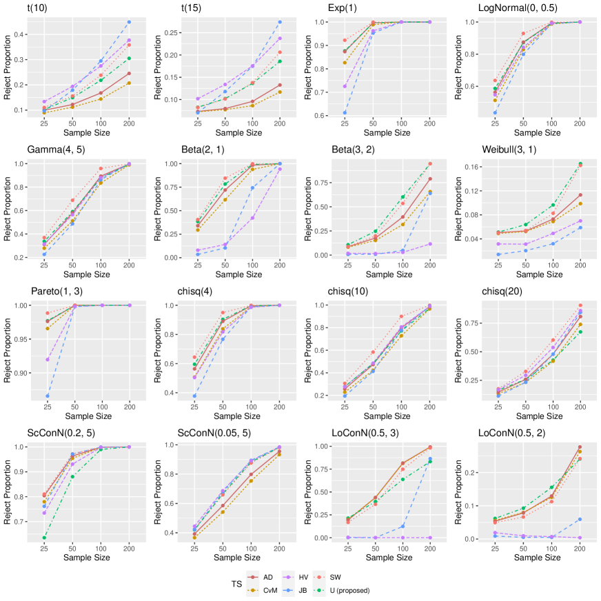
Figure 3: Univariate test under different alternative distributions (continued). Here $R=3$ and $N=500$ for our test statistic.

Figures 2 and 3 compare our proposed tests with other normality tests at different sample sizes. It can be seen that our test outperformed other tests, including the Shapiro-Wilk test, which is often considered as the best univariate normality test, when the true distribution has a bounded support and tend to have performance in between those of other tests in other distributions. Under $H_{0}$ (results not shown in the figures), the sizes of our tests are close to $0.05$, as our test statistic is distribution-free under $H_{0}$ and the critical value is determined using simulation.

For the multivariate case, we compare our proposed test statistic with the following tests: the energy test of Székely and Rizzo (2005), the Henze-Visagie (HV) test (defined in (10)), the Henze–Jiménez-Gamero (HJ) test (Henze and Jiménez-Gamero (2019), the Henze-Zirkler (HZ) test (Henze and Zirkler (1990)) and the Mardia’s test (Mardia (1970)) based on skewness (MS) and kurtosis (MK). A brief description of these tests is as follows. Székely and Rizzo (2005) proposed the test statistic

$$\mathcal{E}_{n}:=n\left(\frac{2}{n}\sum^{n}_{i=1}\mathbb{E}\|Z_{n,i}-X\|-\frac{2\Gamma((p+1)/2)}{\Gamma(p/2)}-\frac{1}{n^{2}}\sum^{n}_{i,j=1}\|Z_{n,i}-Z_{n,j}\|\right),$$

where the first expectation is taking with respect to $X$, which follows $N(0,\textbf{I}_{p})$, and

$$\mathbb{E}(\|a-X\|)=\frac{\sqrt{2}\Gamma(\frac{p+1}{2})}{\Gamma(\frac{p}{2})}+\sqrt{\frac{2}{\pi}}\sum^{\infty}_{k=0}\frac{(-1)^{k}}{k!2^{k}}\frac{\|a\|^{2k+2}}{(2k+1)(2k+2)}\frac{\Gamma(\frac{p+1}{2})\Gamma(k+\frac{3}{2})}{\Gamma(k+\frac{p}{2}+1)}.$$

The test using $\mathcal{E}_{n}$ is known as the energy test and we make use of the function mvnorm.etest in the R package engergy to compute the test statistic and its $p$-value. Székely and Rizzo (2005) concluded that the energy test is a powerful omnibus test having relatively good power against general alternatives compared with other tests. The Henze–Jiménez-Gamero test is based on the test statistic

$$HJ_{n,\beta}:=n\int_{\mathbb{R}^{p}}(M^{(n)}(t)-M(t))^{2}\exp(-\beta\|t\|^{2})dt,$$

where the test rejects $H_{0}$ for large values of $HJ_{n,\beta}$. We include HV and HJ tests for comparison because our test is also based on characterization of normality using a system of partial differential equations involving the moment generating function. It will be of interest to compare the performance of these tests. The Henze-Zirkler test is based on empirical characteristic function of the scaled residuals:

$$HZ_{n,\gamma}:=(2\pi\gamma^{2})^{-p/2}\int_{\mathbb{R}^{d}}\left|\frac{1}{n}\sum^{n}_{j=1}\exp(it^{\top}Z_{n,j})-\exp\left(-\frac{\|t\|^{2}}{2}\right)\right|^{2}\exp\left(-\frac{\|t\|^{2}}{2\gamma^{2}}\right)dt.$$

We compute the test statistics for HV, HJ and HZ tests using the functions HV, HJ, and HZ in the package mnt, respectively. Mardia’s test for multinormality based on sample skewness rejects $H_{0}$ for large values of $b_{1,p}$, where

$$b_{1,p}:=\frac{1}{n^{2}}\sum^{n}_{i,j=1}(Z^{\top}_{n,i}Z_{n,j})^{3}.$$

The sample kurtosis is given by

$$b_{2,p}:=\frac{1}{n}\sum^{n}_{i=1}\|Z_{n,i}\|^{4}.$$

See Mardia (1970) for their limiting null distributions. To perform the tests based on the sample skewness and kurtosis, we use the function mult.norm from the R package QuantPsyc. All the critical values for these multivariate tests are determined from $100,000$ independent replications under the null hypothesis.

For the distributions in the alternative hypothesis, we consider multivariate distributions with independent components where the marginal distributions are the $32$ alternative distributions considered in the univariate case, except for the normal mixture. In addition, we consider dependent multivariate distributions with normal marginals, where the dependence structure is generated from some common copulas, including the Clayton, Gumbel, Frank, Ali–Mikhail–Haq (AMH), and $t$ copulas (see Nelsen (2006)). Except for the $t$ copula, the other copulas are parameterized by one parameter. For $t$ copula, we use the notation tCopula($\rho$, df), where $\rho$ and df denote the parameter in the exchangeable dispersion structure and degrees of freedom, respectively. We also consider the setting where the dependence structure is generated from the Gaussian copula but the marginal distributions are non-normal.

Figure 4 shows the performance of the proposed test with different values of $R$ and $N$ when $n=50$. The results are similar and the test with $R=3$ performed the best over the distributions considered. For the values of $N$, as long as it is not too small, increasing $N$ will not increase the power of the test. Figures 5 and 6 compares the empirical reject proportions of the proposed test to other tests with different dimensions and when $n=50$, $R=3$ and $N=500$. We see that our test performs the best in many different multivariate distributions. Under $H_{0}$, all the tests considered have around $0.05$ sizes as the critical values can be determined by simulation.

More details of the simulation results for both the univariate and multivariate cases are given in the Appendix.

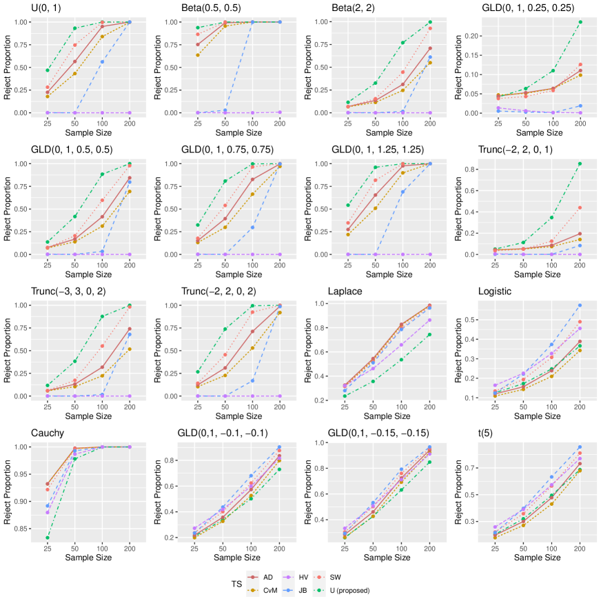
Figure 2: Univariate test under different alternative distributions. Here $R=3$ and $N=500$ for our test statistic.

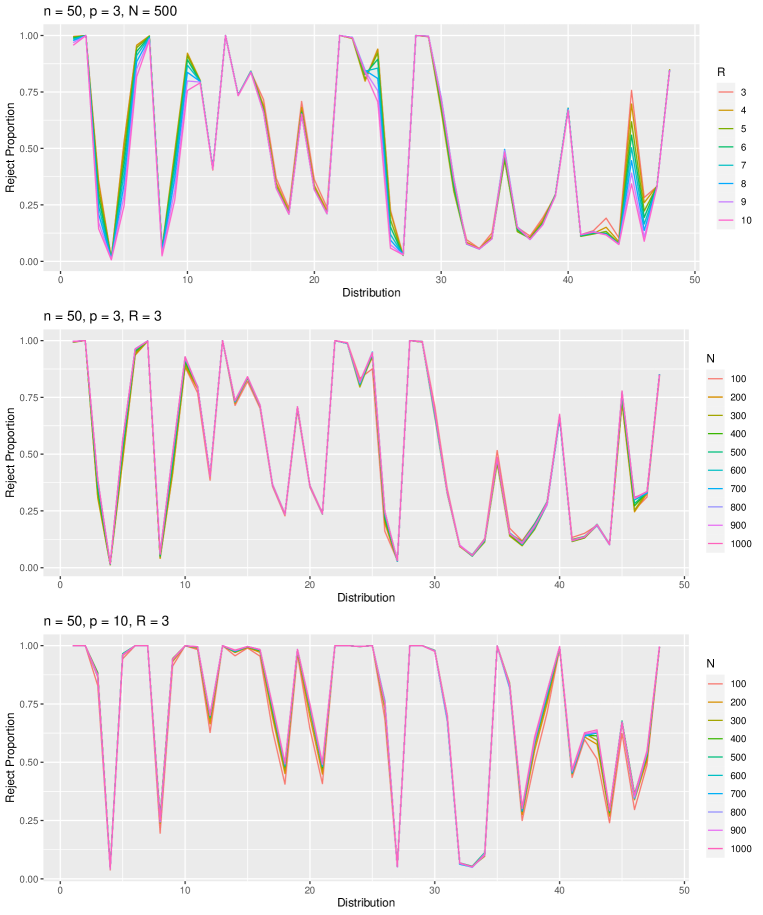
Figure 4: Multivariate test under alternatives when $n=50$. The upper panel shows the empirical reject proportions under the $48$ alternative distributions when $N=500$ and $p=3$ with different values of $R$. The middle panel shows the empirical reject proportions when $R=3$ and $p=3$ with different values of $N$. The lower panel shows the empirical reject proportions when $R=3$ and $p=10$ with different values of $N$.

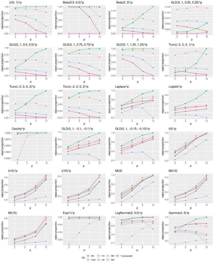
Figure 5: Multivariate test under different alternative distributions and different dimensions $p$ when $n=50$. Here $R=3$ and $N=500$ for our test statistic.

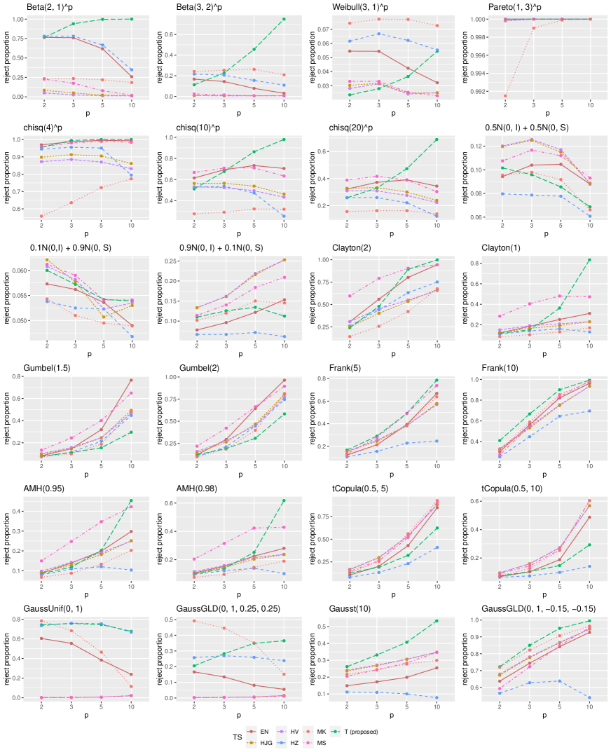
Figure 6: Multivariate test under different alternative distributions and different dimensions $p$ when $n=50$. Here $R=3$ and $N=500$ for our test statistic. $S$ is a matrix with all $0.5$’s in the off-diagonal entries and $1$’s in the diagonal entries.

5 Conclusion

In this article, a novel class of tests for multivariate normality is proposed. Our extensive Monte Carlo study suggested that our test is more powerful in many alternatives compared with existing common tests. We suggest performing our test with $R=3$ and $N=500$, where the set of points can be simulated uniformly from the ball centred at $0$ with radius $R$.

Another possible class of tests can be obtained replacing the moment generating function with the characteristic function in the definition of the cumulant generating function. The finite-sample performance of such a test is undergoing investigation. The idea of combining the dependence structure and marginal information can also be applied to other goodness-of-fit problems.

6 Appendix

To facilitate the proofs, we first define additional notations and describe some of their properties. Let

$$\Delta_{n,i}:=Z_{n,i}-X_{i}=(S^{-1/2}_{n}-\textbf{I}_{p})X_{i}-S^{-1/2}_{n}\overline{X}_{n}.$$ (11)

By Taylor’s theorem, for some $|\theta_{n,i}(t)|\leq 1$, we have

$$e^{t^{\top}\Delta_{n,i}}=1+t^{\top}\Delta_{n,i}+\frac{1}{2}(t^{\top}\Delta_{n,i})^{2}e^{\theta_{n,i}(t)t^{\top}\Delta_{ni}}.$$ (12)

Under $H_{0}$, by (2.13) of Henze and Wagner (1997), we have

$$\sqrt{n}(S^{-1/2}_{n}-\textbf{I}_{p})=-\frac{1}{2\sqrt{n}}\sum^{n}_{i=1}(X_{i}X_{i}^{\top}-\textbf{I}_{p})+O_{p}(n^{-1/2}),$$ (13)

which is $O_{p}(1)$ by the central limit theorem because $\mathbb{E}(X_{i}X_{i}^{\top}-\textbf{I}_{p})=0$. Define $\|\cdot\|_{2}$ to be the spectral norm of a matrix. From (11), we have

$$\|\Delta_{n,i}\|\leq\|(S^{-1/2}_{n}-\textbf{I}_{p})\|_{2}\cdot\|X_{i}\|+\|S^{-1/2}_{n}\|_{2}\cdot\|\overline{X}_{n}\|.$$ (14)

This inequality (14) together with (13) and the fact that $\max_{i=1,\ldots,n}\|X_{i}\|=O_{p}(\log n)$ (see Proposition A.1 in Henze et al. (2019)) imply that

$$\max_{i=1,\ldots,n}\|\Delta_{n,i}\|=O_{p}(n^{-1/2}\log n).$$ (15)

Recall that $M_{0}(t)$ denotes the moment generating function of $X\sim N_{p}(0,\textbf{I}_{p})$. By the strong law of large numbers, for each $t\in\mathbb{R}^{p}$, $M_{n,0}(t)\stackrel{{\scriptstyle a.s.}}{{\rightarrow}}M(t)=e^{\|t\|^{2}/2}$, $\triangledown M_{n,0}(t)\stackrel{{\scriptstyle a.s.}}{{\rightarrow}}\triangledown M_{0}(t)=te^{\|t\|^{2}/2}$, and $H_{M_{n,0}}(t)\stackrel{{\scriptstyle a.s.}}{{\rightarrow}}H_{M_{0}}(t)=(tt^{\top}+\textbf{I}_{p})e^{\|t\|^{2}/2}$. Finally, $\frac{1}{n}\sum^{n}_{i=1}e^{t^{\top}X_{i}}X_{i}X_{i}^{\top}X_{ih}\stackrel{{\scriptstyle a.s.}}{{\rightarrow}}\mathbb{E}(e^{t^{\top}X}XX^{\top}X_{h})$, where $X_{h}$ is the $h$-th component of $X$ and

$$\mathbb{E}(e^{t^{\top}X}XX^{\top}X_{h}) =\frac{\partial}{\partial t_{h}}\mathbb{E}(e^{t^{\top}X}XX^{\top})=\frac{\partial}{\partial t_{h}}\left\{(tt^{\top}+\textbf{I}_{p})e^{\|t\|^{2}/2}\right\}$$

$$=\frac{\partial tt^{\top}}{\partial t_{h}}e^{\|t\|^{2}/2}+tt^{\top}t_{h}e^{\|t\|^{2}/2}+t_{h}e^{\|t\|^{2}/2}\textbf{I}_{p}$$

$$=e^{\|t\|^{2}/2}\left(\frac{\partial tt^{\top}}{\partial t_{h}}+tt^{\top}t_{h}+t_{h}\textbf{I}_{p}\right).$$ (16)

6.1 Proofs for Section 2

Proof of Lemma 1.

1. By (11) and (12),

   $$\sqrt{n}(M^{(n)}(t)-M^{(n)}_{0}(t)) =\frac{1}{\sqrt{n}}\sum^{n}_{i=1}e^{t^{\top}X_{i}}(e^{t^{\top}\Delta_{n,i}}-1)$$

   $$=\frac{1}{\sqrt{n}}\sum^{n}_{i=1}e^{t^{\top}X_{i}}\left\{t^{\top}\Delta_{n,i}+\frac{1}{2}(t^{\top}\Delta_{n,i})^{2}e^{\theta_{n,i}(t)t^{\top}\Delta_{n,i}}\right\}$$

   $$=:A_{1n}+A_{2n}+A_{3n}+A_{4n},$$ (17)

   where

   $$A_{1n} :=\frac{1}{\sqrt{n}}\sum^{n}_{i=1}e^{t^{\top}X_{i}}t^{\top}(S^{-1/2}_{n}-\textbf{I}_{p})X_{i};$$

   $$A_{2n} :=-\frac{1}{\sqrt{n}}\sum^{n}_{i=1}e^{t^{\top}X_{i}}t^{\top}(S^{-1/2}_{n}-\textbf{I}_{p})\overline{X}_{n};$$

   $$A_{3n} :=-\frac{1}{\sqrt{n}}\sum^{n}_{i=1}e^{t^{\top}X_{i}}t^{\top}\overline{X}_{n};$$

   $$A_{4n} :=\frac{1}{\sqrt{n}}\sum^{n}_{i=1}e^{t^{\top}X_{i}}\frac{1}{2}(t^{\top}\Delta_{n,i})^{2}e^{\theta_{n,i}(t)t^{\top}\Delta_{n,i}}.$$

   For $A_{1n}$, we have

   $$A_{1n} =\frac{1}{n}\sum^{n}_{i=1}e^{t^{\top}X_{i}}X_{i}^{\top}\sqrt{n}(S^{-1/2}_{n}-\textbf{I}_{p})t$$

   $$=\left(\frac{1}{n}\sum^{n}_{i=1}e^{t^{\top}X_{i}}X_{i}^{\top}\right)\left\{-\frac{1}{2\sqrt{n}}\sum^{n}_{j=1}(X_{j}X_{j}^{\top}-\textbf{I}_{p})+O_{p}(n^{-1/2})\right\}t$$

   $$=\left(\frac{1}{n}\sum^{n}_{i=1}e^{t^{\top}X_{i}}X_{i}^{\top}\right)\left\{-\frac{1}{2\sqrt{n}}\sum^{n}_{j=1}(X_{j}X_{j}^{\top}-\textbf{I}_{p})\right\}t+o_{p}(1)$$

   $$=e^{\|t\|^{2}/2}t^{\top}\left\{-\frac{1}{2\sqrt{n}}\sum^{n}_{j=1}(X_{j}X_{j}^{\top}-\textbf{I}_{p})\right\}t+o_{p}(1)$$

   $$=-\frac{e^{\|t\|^{2}/2}}{2\sqrt{n}}\sum^{n}_{i=1}\left\{(t^{\top}X_{i})^{2}-\|t\|^{2}\right\}+o_{p}(1),$$ (18)

   where the second equality follows from (13) and the second last equality follows from the weak law of large numbers. For $A_{2n}$, by (13),

   $$A_{2n} =\bigg{(}-\frac{1}{n}\sum^{n}_{i=1}e^{t^{\top}X_{i}}t^{\top}\bigg{)}\sqrt{n}(S^{-1/2}_{n}-\textbf{I}_{p})\overline{X}_{n}$$

   $$=O_{p}(1)O_{p}(1)O_{p}(n^{-1/2})=o_{p}(1).$$ (19)

   For $A_{3n}$, by the weak law of large numbers,

   $$A_{3n} =\bigg{(}-e^{\|t\|^{2}/2}t^{\top}+o_{p}(1)\bigg{)}\sqrt{n}\cdot\overline{X}_{n}=-e^{\|t\|^{2}/2}\frac{1}{\sqrt{n}}\sum^{n}_{i=1}t^{\top}X_{i}+o_{p}(1).$$ (20)

   By (15), we have

   $$A_{4n} \leq\frac{\sqrt{n}}{2}\|t\|^{2}\max_{i=1,\ldots,n}\|\Delta_{n,i}\|^{2}e^{\|t\|\max_{i=1,\ldots,n}\|\Delta_{n,i}\|}\left(\frac{1}{n}\sum^{n}_{i=1}e^{t^{\top}X_{i}}\right)$$

   $$=\sqrt{n}O_{p}(n^{-1}(\log n)^{2})O_{p}(1)O_{p}(1)=o_{p}(1).$$ (21)

   The result then follows from (17)-(21).

2. By (11) and (12),

   $$\sqrt{n}(\triangledown M^{(n)}(t)-\triangledown M^{(n)}_{0}(t))$$

   $$=\frac{1}{\sqrt{n}}\sum^{n}_{i=1}(Z_{n,i}-X_{i})e^{t^{\top}Z_{n,i}}+\frac{1}{\sqrt{n}}\sum^{n}_{i=1}X_{i}\left(e^{t^{\top}Z_{n,i}}-e^{t^{\top}X_{i}}\right)$$

   $$=\frac{1}{\sqrt{n}}\sum^{n}_{i=1}\Delta_{n,i}e^{t^{\top}X_{i}}e^{t^{\top}\Delta_{n,i}}+\frac{1}{\sqrt{n}}\sum^{n}_{i=1}X_{i}e^{t^{\top}X_{i}}(e^{t^{\top}\Delta_{n,i}}-1)$$

   $$=B_{1n}+B_{2n}+B_{3n}+B_{4n},$$ (22)

   where

   $$B_{1n} :=\frac{1}{\sqrt{n}}\sum^{n}_{i=1}(S^{-1/2}_{n}-\textbf{I}_{p})X_{i}e^{t^{\top}X_{i}}e^{t^{\top}\Delta_{n,i}};$$

   $$B_{2n} :=-\frac{1}{\sqrt{n}}\sum^{n}_{i=1}(S^{-1/2}_{n}-\textbf{I}_{p})\overline{X}_{n}e^{t^{\top}X_{i}}e^{t^{\top}\Delta_{n,i}};$$

   $$B_{3n} :=-\frac{1}{\sqrt{n}}\sum^{n}_{i=1}\overline{X}_{n}e^{t^{\top}X_{i}}e^{t^{\top}\Delta_{n,i}};$$

   $$B_{4n} :=\frac{1}{\sqrt{n}}\sum^{n}_{i=1}X_{i}e^{t^{\top}X_{i}}\left\{t^{\top}\Delta_{n,i}+\frac{1}{2}(t^{\top}\Delta_{n,i})^{2}e^{\theta_{n,i}(t)t^{\top}\Delta_{n,i}}\right\}.$$

   By (13) and the weak law of large numbers,

   $$B_{1n} =\frac{1}{n}\sum^{n}_{i=1}\left\{-\frac{1}{2\sqrt{n}}\sum^{n}_{j=1}(X_{j}X_{j}^{\top}-\textbf{I}_{p})\right\}X_{i}e^{t^{\top}X_{i}}+o_{p}(1)$$

   $$=-\frac{1}{2\sqrt{n}}\sum^{n}_{i=1}(X_{i}X_{i}^{\top}-\textbf{I}_{p})\left(te^{\|t\|^{2}/2}+o_{p}(1)\right)+o_{p}(1)$$

   $$=-\frac{e^{\|t\|^{2}/2}}{2\sqrt{n}}\sum^{n}_{i=1}(X_{i}X_{i}^{\top}t-t)+o_{p}(1).$$ (23)

   By (13),

   $$\|B_{2n}\| \leq\left\|\frac{1}{n}\sum^{n}_{i=1}e^{t^{\top}X_{i}}\right\|\|S^{-1/2}_{n}-\textbf{I}_{p}\|_{2}\|\sqrt{n}\cdot\overline{X}_{n}\|e^{\|t\|\max_{i=1,\ldots,n}\|\Delta_{n,i}\|}$$

   $$=O_{p}(1)O_{p}(n^{-1/2})O_{p}(1)O_{p}(1)=o_{p}(1).$$ (24)

   By the weak law of large numbers,

   $$B_{3n} =-\frac{1}{n}\sum^{n}_{i=1}e^{t^{\top}X_{i}}\sqrt{n}\cdot\overline{X}_{n}+o_{p}(1)=-\frac{e^{\|t\|^{2}/2}}{\sqrt{n}}\sum^{n}_{i=1}X_{i}+o_{p}(1).$$ (25)

   Finally, by (11)

   $$B_{4n} =\frac{1}{\sqrt{n}}\sum^{n}_{i=1}X_{i}e^{t^{\top}X_{i}}t^{\top}\Delta_{n,i}+o_{p}(1)$$

   $$=\frac{1}{\sqrt{n}}\sum^{n}_{i=1}X_{i}e^{t^{\top}X_{i}}t^{\top}(S^{-1/2}_{n}-\textbf{I}_{p})X_{i}-\frac{1}{\sqrt{n}}\sum^{n}_{i=1}X_{i}e^{t^{\top}X_{i}}t^{\top}(S^{-1/2}_{n}-\textbf{I}_{p})\overline{X}_{n}$$

   $$\quad-\frac{1}{\sqrt{n}}\sum^{n}_{i=1}X_{i}e^{t^{\top}X_{i}}t^{\top}\overline{X}_{n}+o_{p}(1)$$

   $$=\frac{1}{\sqrt{n}}\sum^{n}_{i=1}e^{t^{\top}X_{i}}X_{i}X^{\top}_{i}(S^{-1/2}_{n}-\textbf{I}_{p})t-te^{\|t\|^{2}/2}\frac{1}{\sqrt{n}}\sum^{n}_{i=1}t^{\top}X_{i}+o_{p}(1)$$

   $$=-\frac{e^{\|t\|^{2}/2}}{2\sqrt{n}}(\textbf{I}_{p}+tt^{\top})\sum^{n}_{i=1}(X_{i}X_{i}^{\top}-\textbf{I}_{p})t-\frac{e^{\|t\|^{2}/2}}{\sqrt{n}}\sum^{n}_{i=1}tt^{\top}X_{i}+o_{p}(1),$$ (26)

   where the last equality follows from (13) and the weak law of large numbers. Combining (22), (23), (24), (25), and (26), we have

   $$\sqrt{n}(\triangledown M^{(n)}(t)-\triangledown M^{(0)}_{0}(t))$$

   $$=\frac{e^{\|t\|^{2}/2}}{\sqrt{n}}\sum^{n}_{i=1}\left\{-\frac{1}{2}(X_{i}X_{i}^{\top}t-t)-X_{i}-\frac{1}{2}(\textbf{I}_{p}+tt^{\top})(X_{i}X_{i}^{\top}-\textbf{I}_{p})t-tt^{\top}X_{i}\right\}+o_{p}(1)$$

   $$=\frac{e^{\|t\|^{2}/2}}{\sqrt{n}}\sum^{n}_{i=1}\left\{-(\textbf{I}_{p}+tt^{\top})X_{i}-\frac{1}{2}(2\textbf{I}_{p}+tt^{\top})(X_{i}X_{i}^{\top}-\textbf{I}_{p})t\right\}+o_{p}(1).$$

3. Note that

   $$Z_{n,i}Z_{n,i}^{\top}-X_{i}X_{i}^{\top} =(\Delta_{n,i}+X_{i})(\Delta_{n,i}+X_{i})^{\top}-X_{i}X_{i}^{\top}$$

   $$=\Delta_{n,i}\Delta^{\top}_{n,i}+\Delta_{n,i}X^{\top}_{i}+X_{i}\Delta^{\top}_{n,i}.$$

   Thus,

   $$\sqrt{n}(H_{M^{(n)}}(t)-H_{M^{(n)}_{0}}(t))$$

   $$=\frac{1}{\sqrt{n}}\sum^{n}_{i=1}(Z_{n,i}Z_{n,i}^{\top}-X_{i}X_{i}^{\top})e^{t^{\top}X_{i}}e^{t^{\top}\Delta_{n,i}}+\frac{1}{\sqrt{n}}\sum^{n}_{i=1}X_{i}X_{i}^{\top}e^{t^{\top}X_{i}}(e^{t^{\top}\Delta_{n,i}}-1)$$

   $$=C_{1n}+C_{2n}+C_{3n}+C_{4n},$$

   where

   $$C_{1n} :=\frac{1}{\sqrt{n}}\sum^{n}_{i=1}\Delta_{n,i}\Delta_{n,i}^{\top}e^{t^{\top}X_{i}}e^{t^{\top}\Delta_{n,i}};$$

   $$C_{2n} :=\frac{1}{\sqrt{n}}\sum^{n}_{i=1}\Delta_{n,i}X^{\top}_{i}e^{t^{\top}X_{i}}e^{t^{\top}\Delta_{n,i}};$$

   $$C_{3n} :=\frac{1}{\sqrt{n}}\sum^{n}_{i=1}X_{i}\Delta_{n,i}^{\top}e^{t^{\top}X_{i}}e^{t^{\top}\Delta_{n,i}};$$

   $$C_{4n} :=\frac{1}{\sqrt{n}}\sum^{n}_{i=1}X_{i}X_{i}^{\top}e^{t^{\top}X_{i}}\left\{t^{\top}\Delta_{n,i}+\frac{1}{2}(t^{\top}\Delta_{n,i})^{2}e^{\theta_{n,i}(t)t^{\top}\Delta_{n,i}}\right\}.$$

   For $C_{1n}$, by (15),

   $$\|C_{1n}\|_{2} \leq\sqrt{n}\left|\frac{1}{n}\sum^{n}_{i=1}e^{t^{\top}X_{i}}\right|\max_{i=1,\ldots,n}\|\Delta_{n,i}\|^{2}e^{\|t\|\max_{i=1,\ldots,n}\|\Delta_{n,i}\|}$$

   $$=\sqrt{n}O_{p}(1)O_{p}(n^{-1}(\log n)^{2})O_{p}(1)=o_{p}(1).$$

   For $C_{2n}$, by (13),

   $$C_{2n} =\frac{1}{\sqrt{n}}\sum^{n}_{i=1}(S^{-1/2}_{n}-\textbf{I}_{p})X_{i}X_{i}^{\top}e^{t^{\top}X_{i}}-\frac{1}{\sqrt{n}}\sum^{n}_{i=1}(S^{-1/2}_{n}-\textbf{I}_{p})\overline{X}_{n}X_{i}^{\top}e^{t^{\top}X_{i}}$$

   $$\quad-\frac{1}{\sqrt{n}}\sum^{n}_{i=1}\overline{X}_{n}X_{i}^{\top}e^{t^{\top}X_{i}}+o_{p}(1)$$

   $$=\frac{1}{n}\sum^{n}_{i=1}\left\{-\frac{1}{2\sqrt{n}}\sum^{n}_{j=1}(X_{j}X_{j}^{\top}-\textbf{I}_{p})+O_{p}(n^{-1/2})\right\}X_{i}X_{i}^{\top}e^{t^{\top}X_{i}}+O_{p}(n^{-1/2})$$

   $$\quad-\frac{1}{\sqrt{n}}\sum^{n}_{i=1}X_{i}\left(t^{\top}e^{\|t\|^{2}/2}+o_{p}(1)\right)+o_{p}(1)$$

   $$=-\frac{1}{2\sqrt{n}}\sum^{n}_{i=1}(X_{i}X_{i}^{\top}-\textbf{I}_{p})e^{\|t\|^{2}/2}(\textbf{I}_{p}+tt^{\top}+o_{p}(1))-\frac{e^{\|t\|^{2}/2}}{\sqrt{n}}\sum^{n}_{i=1}X_{i}t^{\top}+o_{p}(1)$$

   $$=-\frac{e^{\|t\|^{2}/2}}{2\sqrt{n}}\sum^{n}_{i=1}(X_{i}X_{i}^{\top}-\textbf{I}_{p})(\textbf{I}_{p}+tt^{\top})-\frac{e^{\|t\|^{2}/2}}{\sqrt{n}}\sum^{n}_{i=1}X_{i}t^{\top}+o_{p}(1).$$

   Since $C_{3n}=C_{2n}^{\top}$, we have

   $$C_{3n}=-\frac{e^{\|t\|^{2}/2}}{2\sqrt{n}}\sum^{n}_{i=1}(\textbf{I}_{p}+tt^{\top})(X_{i}X_{i}^{\top}-\textbf{I}_{p})-\frac{e^{\|t\|^{2}/2}}{\sqrt{n}}\sum^{n}_{i=1}tX^{\top}_{i}+o_{p}(1).$$

   For $C_{4n}$,

   $$C_{4n} =\frac{1}{\sqrt{n}}\sum^{n}_{i=1}X_{i}X_{i}^{\top}e^{t^{\top}X_{i}}t^{\top}(S^{-1/2}_{n}-\textbf{I}_{p})X_{i}-\frac{1}{\sqrt{n}}\sum^{n}_{i=1}X_{i}X_{i}^{\top}e^{t^{\top}X_{i}}t^{\top}(S^{-1/2}_{n}-\textbf{I}_{p})\overline{X}_{n}$$

   $$\quad-\frac{1}{\sqrt{n}}\sum^{n}_{i=1}X_{i}X_{i}^{\top}e^{t^{\top}X_{i}}t^{\top}\overline{X}_{n}+o_{p}(1)$$

   $$=\frac{1}{n}\sum^{n}_{i=1}e^{t^{\top}X_{i}}X_{i}X_{i}^{\top}X^{\top}_{i}\left\{-\frac{1}{2\sqrt{n}}\sum^{n}_{j=1}(X_{j}X_{j}^{\top}-\textbf{I}_{p})+O_{p}(n^{-1/2})\right\}t+O_{p}(n^{-1/2})$$

   $$\quad-\frac{e^{\|t\|^{2}/2}}{\sqrt{n}}(\textbf{I}_{p}+tt^{\top})\sum^{n}_{i=1}t^{\top}X_{i}+o_{p}(1)$$

   $$=\frac{1}{n}\sum^{n}_{i=1}e^{t^{\top}X_{i}}X_{i}X_{i}^{\top}X^{\top}_{i}\left\{-\frac{1}{2\sqrt{n}}\sum^{n}_{j=1}(X_{j}X_{j}^{\top}-\textbf{I}_{p})\right\}t-\frac{e^{\|t\|^{2}/2}}{\sqrt{n}}(\textbf{I}_{p}+tt^{\top})\sum^{n}_{i=1}t^{\top}X_{i}$$

   $$\quad+o_{p}(1).$$

   Denote $\tilde{C}_{n}:=-\frac{1}{2\sqrt{n}}\sum^{n}_{j=1}(X_{j}X_{j}^{\top}-\textbf{I}_{p})$. Note that

   $$\frac{1}{n}\sum^{n}_{i=1}e^{t^{\top}X_{i}}X_{i}X_{i}^{\top}X^{\top}_{i}\tilde{C}_{n}t$$

   $$=\frac{1}{n}\sum^{n}_{i=1}e^{t^{\top}X_{i}}X_{i}X_{i}^{\top}\sum^{p}_{h=1}\sum^{p}_{k=1}X_{ih}\tilde{C}_{n,hk}t_{k}$$

   $$=\sum^{p}_{h=1}\left\{\left(\frac{1}{n}\sum^{n}_{i=1}e^{t^{\top}X_{i}}X_{i}X_{i}^{\top}X_{ih}\right)\sum^{p}_{k=1}t_{k}\tilde{C}_{n,hk}\right\}$$

   $$=\sum^{p}_{h=1}\left\{\mathbb{E}(e^{t^{\top}X}XX^{\top}X_{h})\sum^{p}_{k=1}t_{k}\tilde{C}_{n,hk}\right\}+o_{p}(1)$$

   $$=-\frac{1}{2\sqrt{n}}\sum^{n}_{i=1}\left\{\sum^{p}_{h=1}\sum^{p}_{k=1}\mathbb{E}(e^{t^{\top}X}XX^{\top}X_{h})t_{k}(X_{ih}X_{ik}-\mathbbm{1}(h=k))\right\}+o_{p}(1).$$

   Thus, by (16),

   $$C_{4n} =-\frac{e^{\|t\|^{2}/2}}{2\sqrt{n}}\sum^{n}_{i=1}\left\{\sum^{p}_{h=1}\sum^{p}_{k=1}\left(\frac{\partial tt^{\top}}{\partial t_{h}}+tt^{\top}t_{h}+t_{h}\textbf{I}_{p}\right)t_{k}(X_{ih}X_{ik}-\mathbbm{1}(h=k))\right\}$$

   $$\quad-\frac{e^{\|t\|^{2}/2}}{\sqrt{n}}(\textbf{I}_{p}+tt^{\top})\sum^{n}_{i=1}t^{\top}X_{i}+o_{p}(1).$$

∎

Proof of Lemma 2.

1. We can write

   $$M^{(n)}_{0}(t)H_{M^{(n)}_{0}}(t)-\triangledown M^{(n)}_{0}(t)(\triangledown M^{(n)}_{0}(t))^{\top}-(M^{(n)}_{0}(t))^{2}\textbf{I}_{p}=E_{1n}+E_{2n}+E_{3n},$$

   where

   $$E_{1n} :=M_{0}(t)H_{M^{(n)}_{0}}(t)-\triangledown M_{0}(t)(\triangledown M^{(n)}_{0}(t))^{\top}-M_{0}(t)M^{(n)}_{0}(t)\textbf{I}_{p};$$

   $$E_{2n} :=\{M^{(n)}_{0}(t)-M_{0}(t)\}H_{M_{0}}(t)-\{\triangledown M^{(n)}_{0}(t)-\triangledown M_{0}(t)\}(\triangledown M_{0}(t))^{\top}$$

   $$\quad-\{M^{(n)}_{0}(t)-M_{0}(t)\}M_{0}(t)\textbf{I}_{p};$$

   $$E_{3n} :=\{M^{(n)}_{0}(t)-M_{0}(t)\}\{H_{M^{(n)}_{0}}(t)-H_{M_{0}}(t)\}$$

   $$\quad-\{\triangledown M^{(n)}_{0}(t)-\triangledown M_{0}(t)\}\{\triangledown M^{(n)}_{0}(t)-\triangledown M_{0}(t)\}^{\top}$$

   $$\quad-\{M^{(n)}_{0}(t)-M_{0}(t)\}\{M^{(n)}_{0}(t)-M_{0}(t)\}\textbf{I}_{p}.$$

   For $E_{1n}$, we have

   $$E_{1n} =\frac{1}{n}\sum^{n}_{i=1}\bigg{(}e^{\|t\|^{2}/2}X_{i}X_{i}^{\top}e^{t^{\top}X_{i}}-e^{\|t\|^{2}/2}tX_{i}^{\top}e^{t^{\top}X_{i}}-e^{\|t\|^{2}/2}e^{t^{\top}X_{i}}\textbf{I}_{p}\bigg{)}$$

   $$=\frac{e^{\|t\|^{2}/2}}{n}\sum^{n}_{i=1}e^{t^{\top}X_{i}}(X_{i}X_{i}^{\top}-tX_{i}^{\top}-\textbf{I}_{p}).$$

   For $E_{2n}$, we have

   $$E_{2n} :=\frac{1}{n}\sum^{n}_{i=1}(e^{t^{\top}X_{i}}-e^{\|t\|^{2}/2})\{H_{M_{0}}(t)-M_{0}(t)\textbf{I}_{p}\}$$

   $$\quad-\frac{1}{n}\sum^{n}_{i=1}(X_{i}e^{t^{\top}X_{i}}-te^{\|t\|^{2}/2})(\triangledown M_{0}(t))^{\top}$$

   $$=\frac{e^{\|t\|^{2}/2}}{n}\sum^{n}_{i=1}\left\{(e^{t^{\top}X_{i}}-e^{\|t\|^{2}/2})tt^{\top}-(X_{i}t^{\top}e^{t^{\top}X_{i}}-tt^{\top}e^{\|t\|^{2}/2})\right\}$$

   $$=\frac{e^{\|t\|^{2}/2}}{n}\sum^{n}_{i=1}\left\{e^{t^{\top}X_{i}}(tt^{\top}-X_{i}t^{\top})\right\}.$$

   By Lemma 1, $E_{3n}=O_{p}(n^{-1})$. Thus, the result follows.

2. Denote $F_{1n}:=M^{(n)}(t)H_{M^{(n)}}(t)$, $F_{2n}:=\triangledown M^{(n)}(t)(\triangledown M^{(n)}(t))^{\top}$ and $F_{3n}:=(M^{(n)}(t))^{2}\textbf{I}_{p}$. Then,

   $$M^{(n)}(t)H_{M^{(n)}}(t)-\triangledown M^{(n)}(t)(\triangledown M^{(n)}(t))^{\top}-(M^{(n)}(t))^{2}\textbf{I}_{p}=F_{1n}-F_{2n}-F_{3n}.$$

   Recall that $\mathbb{E}(f_{j}(X_{i};t))=0$, by the central limit theorem $n^{-1}\sum^{n}_{i=1}f_{j}(X_{i};t)=O_{p}(n^{-1/2})$ for $j=0,1,2$. By Lemma 1,

   $$F_{1n} =\left(M^{(n)}_{0}(t)+\frac{1}{n}\sum^{n}_{i=1}f_{0}(X_{i};t)+o_{p}(n^{-1/2})\right)\left(H_{M^{(n)}_{0}}(t)+\frac{1}{n}\sum^{n}_{i=1}f_{2}(X_{i};t)+o_{p}(n^{-1/2})\right)$$

   $$=M^{(n)}_{0}(t)H_{M^{(n)}_{0}}(t)+M^{(n)}_{0}(t)\left(\frac{1}{n}\sum^{n}_{i=1}f_{2}(X_{i};t)\right)+\left(\frac{1}{n}\sum^{n}_{i=1}f_{0}(X_{i};t)\right)H_{M^{(n)}_{0}}(t)+o_{p}(n^{-1/2})$$

   $$=M^{(n)}_{0}(t)H_{M^{(n)}_{0}}(t)+M_{0}(t)\left(\frac{1}{n}\sum^{n}_{i=1}f_{2}(X_{i};t)\right)+\left(\frac{1}{n}\sum^{n}_{i=1}f_{0}(X_{i};t)\right)H_{M_{0}}(t)+o_{p}(n^{-1/2}),$$

   where the last equality holds as $(M^{(n)}_{0}(t)-M_{0}(t))\left(n^{-1}\sum^{n}_{i=1}f_{2}(X_{i};t)\right)=O_{p}(n^{-1/2})O_{p}(n^{-1/2})=O_{p}(n^{-1})$ and $\left(n^{-1}\sum^{n}_{i=1}f_{0}(X_{i};t)\right)(H_{M^{(n)}_{0}}(t)-H_{M_{0}}(t))=O_{p}(n^{-1/2})O_{p}(n^{-1/2})=O_{p}(n^{-1})$, by the central limit theorem. Thus,

   $$F_{1n}=M^{(n)}_{0}(t)H_{M^{(n)}_{0}}(t)+\frac{e^{\|t\|^{2}/2}}{n}\sum^{n}_{i=1}\left\{f_{2}(X_{i};t)+(tt^{\top}+\textbf{I}_{p})f_{0}(X_{i};t)\right\}+o_{p}(n^{-1/2}).$$ (27)

   Similarly, by Lemma 1,

   $$F_{2n} =\left(\triangledown M^{(n)}_{0}(t)+\frac{1}{n}\sum^{n}_{i=1}f_{1}(X_{i};t)+o_{p}(n^{-1/2})\right)$$

   $$\quad\quad\left(\triangledown M^{(n)}_{0}(t)+\frac{1}{n}\sum^{n}_{i=1}f_{1}(X_{i};t)+o_{p}(n^{-1/2})\right)^{\top}$$

   $$=\triangledown M^{(n)}_{0}(t)(\triangledown M^{(n)}_{0}(t))^{\top}+\triangledown M^{(n)}_{0}(t)\left(\frac{1}{n}\sum^{n}_{i=1}f_{1}(X_{i};t)^{\top}\right)$$

   $$\quad+\left(\frac{1}{n}\sum^{n}_{i=1}f_{1}(X_{i};t)\right)(\triangledown M^{(n)}_{0}(t))^{\top}+o_{p}(n^{-1/2})$$

   $$=\triangledown M^{(n)}_{0}(t)(\triangledown M^{(n)}_{0}(t))^{\top}+\triangledown M_{0}(t)\left(\frac{1}{n}\sum^{n}_{i=1}f_{1}(X_{i};t)^{\top}\right)$$

   $$\quad+\left(\frac{1}{n}\sum^{n}_{i=1}f_{1}(X_{i};t)\right)(\triangledown M_{0}(t))^{\top}+o_{p}(n^{-1/2}).$$

   Thus,

   $$F_{n2}=\triangledown M^{(n)}_{0}(t)(\triangledown M^{(n)}_{0}(t))^{\top}+\frac{e^{\|t\|^{2}/2}}{n}\sum^{n}_{i=1}\left(tf^{\top}_{1}(X_{i};t)+f_{1}(X_{i};t)t^{\top}\right)+o_{p}(n^{-1/2}).$$ (28)

   Using the same argument, we have

   $$F_{3n} =\left(M^{(n)}_{0}(t)+\frac{1}{n}\sum^{n}_{i=1}f_{0}(X_{i};t)+o_{p}(n^{-1/2})\right)^{2}\textbf{I}_{p}$$

   $$=\left(\left(M^{(n)}_{0}(t)\right)^{2}+\frac{2M^{(n)}_{0}(t)}{n}\sum^{n}_{i=1}f_{0}(X_{i};t)+o_{p}(n^{-1/2})\right)\textbf{I}_{p}$$

   $$=\left(M^{(n)}_{0}(t)\right)^{2}\textbf{I}_{p}+\frac{e^{\|t\|^{2}/2}}{n}\sum^{n}_{i=1}(2f_{0}(X_{i};t)\textbf{I}_{p})+o_{p}(n^{-1/2}).$$ (29)

   The result follows by combining (27), (28), and (29) and part (a) of this lemma.

∎

Proof of Theorem 1.

By Lemma 1 (a) and Lemma 2 (b), we have

$$\sqrt{n}(H_{\Lambda_{n}}(t)-\textbf{I}_{p})$$

$$=(M^{(n)}(t))^{-2}\sqrt{n}\{M^{(n)}(t)H_{M^{(n)}}(t)-\triangledown M^{(n)}(t)(\triangledown M^{(n)}(t))^{\top}-(M^{(n)})^{2}(t)\textbf{I}_{p}\}$$

$$=M^{-2}_{0}(t)\sqrt{n}\{M^{(n)}(t)H_{M^{(n)}}(t)-\triangledown M^{(n)}(t)(\triangledown M^{(n)}(t))^{\top}-(M^{(n)})^{2}(t)\textbf{I}_{p}\}$$

$$\quad+\{(M^{(n)}(t))^{-2}-M^{-2}_{0}(t)\}\sqrt{n}\{M^{(n)}(t)H_{M^{(n)}}(t)-\triangledown M^{(n)}(t)(\triangledown M^{(n)}(t))^{\top}-(M^{(n)})^{2}(t)\textbf{I}_{p}\}$$

$$=\frac{1}{\sqrt{n}}\sum^{n}_{i=1}h(X_{i};t)+o_{p}(1)+O_{p}(n^{-1/2})O_{p}(1).$$

Thus, the results follow. ∎

6.2 Proofs for Section 3

The following lemma is a generalization of Proposition 5 in Henze and Visagie (2020), where that proposition corresponds to the case when $A=\textbf{I}_{p}$.

Lemma 3.

Let $A_{n}$ be a sequence of $p\times p$ symmetric positive definite matrices, $A$ be a $p\times p$ symmetric positive definite matrix, and $b_{n}$ be an increasing sequence of positive real numbers satisfying $\lim_{n\to\infty}b_{n}=\infty$. Suppose that $\lim_{n\to\infty}b_{n}\|A_{n}-A\|_{2}=0$, then

$$\lim_{n\to\infty}b_{n}\|A_{n}^{-1/2}-A^{-1/2}\|_{2}=0.$$

Proof of Lemma 3.

Note that

$$A_{n}-A= ~{}(A_{n}^{1/2}+A^{1/2})(A_{n}^{1/2}-A^{1/2})$$

$$= ~{}(A_{n}^{1/2}+A^{1/2})A_{n}^{1/2}(A^{-1/2}-A_{n}^{-1/2})A^{1/2}.$$

Thus, we have

$$b_{n}\|A^{-1/2}-A_{n}^{-1/2}\|_{2}\leq\|A_{n}^{-1/2}\|_{2}\cdot\|(A_{n}^{1/2}+A^{1/2})^{-1}\|_{2}\cdot\|A^{-1/2}\|_{2}\cdot(b_{n}\|A_{n}-A\|_{2}).$$ (30)

Since $\lim_{n\rightarrow\infty}b_{n}\|A_{n}-A\|_{2}=0$, it remains to show that the other terms on the RHS of (30) are bounded. Clearly, $\|A^{-1/2}\|_{2}<\infty$. Denote $\lambda_{\min}(B)$ to be the smallest eigenvalue of a matrix $B$. Let $\lambda_{1}:=\lambda_{\min}(A)>0$ since $A$ is positive definite. Since $\|\cdot\|_{2}$ is the spectral norm, by Weyl’s inequality, we have

$$\|(A_{n}^{1/2}+A^{1/2})^{-1}\|_{2}=\frac{1}{\lambda_{\min}\left(A^{1/2}_{n}+A^{1/2}\right)}\leq\frac{1}{\lambda_{\min}(A^{1/2}_{n})+\lambda_{1}^{1/2}}\leq\frac{1}{\lambda^{1/2}_{1}}<\infty.$$ (31)

Let $F_{n}:=A-A_{n}$. Since $\lim_{n\rightarrow\infty}b_{n}\|A_{n}-A\|_{2}=0$, there exists $n_{0}\in\mathbb{N}$ such that for all $n\geq n_{0}$, $\|F_{n}\|_{2}=\|A_{n}-A\|_{2}\leq\lambda_{1}/2$. For all $n\geq n_{0}$, by Weyl’s inequality again,

$$\|A_{n}^{-1}\|_{2}= ~{}\frac{1}{\lambda_{\min}(A_{n})}=\frac{1}{\lambda_{\min}(A-F_{n})}\leq\frac{1}{\lambda_{1}+\lambda_{\min}(-F_{n})}$$

$$\leq ~{}\frac{1}{\lambda_{1}-\|F_{n}\|_{2}}\leq\frac{1}{\lambda_{1}-\lambda_{1}/2}=\frac{2}{\lambda_{1}}<\infty.$$

This implies that $\|A_{n}^{-1/2}\|_{2}\leq\sqrt{2/\lambda_{1}}<\infty$ for all $n\geq n_{0}$. ∎

Let $\tilde{X}_{i}:=\Sigma^{-1/2}X_{i}$ for $i=1,\ldots,n$. Denote $\tilde{M}^{(n)}(t):=\frac{1}{n}\sum^{n}_{i=1}e^{t^{\top}\tilde{X}_{i}}$, $\triangledown\tilde{M}^{(n)}(t):=\frac{1}{n}\sum^{n}_{i=1}\tilde{X}_{i}e^{t^{\top}\tilde{X}_{i}}$ and $H_{\tilde{M}^{(n)}}(t):=\frac{1}{n}\sum^{n}_{i=1}\tilde{X}_{i}\tilde{X}_{i}e^{t^{\top}\tilde{X}_{i}}$.

Lemma 4.

Suppose that the moment generating function of $X$ exists and is twice differentiable. We have

1. $M^{(n)}(t)-\tilde{M}^{(n)}(t)\stackrel{{\scriptstyle a.s.}}{{\rightarrow}}0$;

2. $\|\triangledown M^{(n)}(t)-\triangledown\tilde{M}^{(n)}(t)\|\stackrel{{\scriptstyle a.s.}}{{\rightarrow}}0$;

3. $\|H_{M^{(n)}}(t)-H_{\tilde{M}^{(n)}}(t)\|_{2}\stackrel{{\scriptstyle a.s.}}{{\rightarrow}}0$.

Proof of Lemma 4.

Define

$$\tilde{\Delta}_{n,i}:=Z_{n,i}-\tilde{X}_{i}=(S^{-1/2}_{n}-\Sigma^{-1/2})X_{i}-S^{-1/2}_{n}\overline{X}_{n}.$$

Let $\xi_{n}:=\max_{i=1,\ldots,n}\|\tilde{\Delta}_{n,i}\|$. Then,

$$\xi_{n}\leq n^{1/4}\|S^{-1/2}_{n}-\Sigma^{-1/2}\|_{2}\cdot n^{-1/4}\max_{i=1,\ldots,n}\|X_{j}\|+\|S^{-1/2}_{n}\|_{2}\|\overline{X}_{n}\|.$$ (32)

Since the existence of the moment generating function implies that $\mathbb{E}\|X\|^{4}<\infty$, Theorem 5.2 of Barndorff-Nielsen (1963) gives $n^{-1/4}\max_{i=1,\ldots,n}\|X_{i}\|\rightarrow 0$ almost surely. As $S_{n}-\Sigma=n^{-1}\sum^{n}_{i=1}(X_{i}X_{i}^{\top}-\textbf{I}_{p})-\overline{X}_{n}\overline{X}^{\top}_{n}$, Kolmogorov’s variance criterion for averages (see Kallenberg (2021) p.113) implies that $n^{1/2-\varepsilon}\|S_{n}-\Sigma\|_{2}\rightarrow 0$ almost surely for any $\varepsilon>0$. Lemma 3 then yields $n^{1/2-\varepsilon}\|S^{-1/2}_{n}-\Sigma^{-1/2}\|_{2}\rightarrow 0$ almost surely. From the proof of Lemma 3, we also know that $\sup_{n\geq 1}\|S^{-1/2}_{n}\|_{2}<\infty$ almost surely. By the strong law of large numbers, $\|\overline{X}_{n}\|\rightarrow 0$ almost surely. In view of (32), with probability one,

$$\xi_{n}\leq o(n^{-1/4+\varepsilon})o(1)+o(1)=o(1)$$

for $\varepsilon<1/4$. Thus,

$$\lim_{n\rightarrow\infty}\xi_{n}=0,\quad\text{a.s.}$$ (33)

By Taylor’s theorem, for some $|\theta_{n,i}(t)|\leq 1$, we have

$$e^{t^{\top}\tilde{\Delta}_{n,i}}=1+t^{\top}\tilde{\Delta}_{n,i}+\frac{1}{2}(t^{\top}\tilde{\Delta}_{n,i})^{2}e^{\theta_{n,i}(t)t^{\top}\tilde{\Delta}_{n,i}}.$$ (34)

By (34),

$$M^{(n)}(t)-\tilde{M}^{(n)}(t) =\frac{1}{n}\sum^{n}_{i=1}e^{t^{\top}\tilde{X}_{i}}(e^{t^{\top}\tilde{\Delta}_{n,i}}-1)$$

$$=\frac{1}{n}\sum^{n}_{i=1}e^{t^{\top}\tilde{X}_{i}}\left\{t^{\top}\tilde{\Delta}_{n,i}+\frac{1}{2}(t^{\top}\tilde{\Delta}_{n,i})^{2}e^{\theta_{n,i}(t)t^{\top}\tilde{\Delta}_{n,i}}\right\}.$$

Thus, as $\xi_{n}=\max_{i=1,\ldots,n}\|\tilde{\Delta}_{n,i}\|$,

$$|M^{(n)}(t)-\tilde{M}^{(n)}(t)| \leq\left|\tilde{M}^{(n)}(t)\right|\max_{i=1,\ldots,n}\left|t^{\top}\tilde{\Delta}_{n,i}+\frac{1}{2}(t^{\top}\tilde{\Delta}_{n,i})^{2}e^{\theta_{n,i}(t)t^{\top}\tilde{\Delta}_{n,i}}\right|$$

$$\leq\left|\tilde{M}^{(n)}(t)\right|\max_{i=1,\ldots,n}\bigg{(}\|t\|\cdot\|\tilde{\Delta}_{n,i}\|+\frac{1}{2}\|t\|^{2}\cdot\|\tilde{\Delta}_{n,i}\|^{2}e^{\theta_{n,i}(t)\|t\|\cdot\|\tilde{\Delta}_{n,i}\|}\bigg{)}$$

$$\leq\left|\tilde{M}^{(n)}(t)\right|\bigg{(}\|t\|\xi_{n}+\frac{1}{2}\|t\|^{2}\xi_{n}^{2}e^{\|t\|\xi_{n}}\bigg{)}.$$ (35)

Recall that $\tilde{M}(t):=\mathbb{E}(e^{t^{\top}\tilde{X}})$. By the strong law of large numbers, $\tilde{M}^{(n)}(t)\stackrel{{\scriptstyle a.s.}}{{\rightarrow}}\tilde{M}(t)$. Combining (35) and (33), we deduce that

$$M^{(n)}(t)-\tilde{M}^{(n)}(t)\stackrel{{\scriptstyle a.s.}}{{\rightarrow}}0.$$ (36)

Similarly, using (34), we have

$$\triangledown M^{(n)}(t)-\triangledown\tilde{M}^{(n)}(t)$$

$$=\frac{1}{n}\sum^{n}_{i=1}(Z_{n,i}-\tilde{X}_{i})e^{t^{\top}Z_{n,i}}+\frac{1}{n}\sum^{n}_{i=1}\tilde{X}_{i}(e^{t^{\top}Z_{n,i}}-e^{t^{\top}\tilde{X}_{i}})$$

$$=\frac{1}{n}\sum^{n}_{i=1}e^{t^{\top}\tilde{X}_{i}}\tilde{\Delta}_{n,i}\cdot e^{t^{\top}\tilde{\Delta}_{n,i}}+\frac{1}{n}\sum^{n}_{i=1}\tilde{X}_{i}e^{t^{\top}\tilde{X}_{i}}\left\{t^{\top}\tilde{\Delta}_{n,i}+\frac{1}{2}(t^{\top}\tilde{\Delta}_{n,i})^{2}e^{\theta_{n,i}(t)t^{\top}\tilde{\Delta}_{n,i}}\right\}.$$

By the facts that $\tilde{M}^{(n)}(t)\stackrel{{\scriptstyle a.s.}}{{\rightarrow}}\tilde{M}(t)$, $\|\triangledown\tilde{M}^{(n)}(t)\|\stackrel{{\scriptstyle a.s.}}{{\rightarrow}}\|\triangledown\tilde{M}(t)\|$, and (33), we obtain that

$$\left\|\triangledown M^{(n)}(t)-\triangledown\tilde{M}^{(n)}(t)\right\|$$

$$\leq|\tilde{M}^{(n)}(t)|\max_{i=1,\ldots,n}\|\tilde{\Delta}_{n,i}e^{t^{\top}\tilde{\Delta}_{n,i}}\|+\|\triangledown\tilde{M}_{n}(t)\|\max_{i=1,\ldots,n}\left|t^{\top}\tilde{\Delta}_{n,i}+\frac{1}{2}(t^{\top}\tilde{\Delta}_{n,i})^{2}e^{\theta_{n,i}(t)t^{\top}\tilde{\Delta}_{n,i}}\right|$$

$$\leq|\tilde{M}^{(n)}(t)|\xi_{n}e^{\|t\|\xi_{n}}+\|\triangledown\tilde{M}_{n}(t)\|\left(\|t\|\xi_{n}+\frac{1}{2}\|t\|^{2}\xi_{n}^{2}e^{\|t\|\xi_{n}}\right)\stackrel{{\scriptstyle a.s}}{{\rightarrow}}0.$$

Similar to the proof of Lemma 1, we expand

$$H_{M^{(n)}}(t)-H_{\tilde{M}^{(n)}}(t) =:J_{1n}+J_{2n}+J_{3n}+J_{4n},$$

where

$$J_{1n} :=\frac{1}{n}\sum^{n}_{i=1}\tilde{\Delta}_{n,i}\tilde{\Delta}_{n,i}^{\top}e^{t^{\top}\tilde{X}_{i}}e^{t^{\top}\tilde{\Delta}_{n,i}};$$

$$J_{2n} :=\frac{1}{n}\sum^{n}_{i=1}\tilde{\Delta}_{n,i}\tilde{X}_{i}^{\top}e^{t^{\top}\tilde{X}_{i}}e^{t^{\top}\tilde{\Delta}_{n,i}};$$

$$J_{3n} :=\frac{1}{n}\sum^{n}_{i=1}\tilde{X}_{i}\tilde{\Delta}_{n,i}^{\top}e^{t^{\top}\tilde{X}_{i}}e^{t^{\top}\tilde{\Delta}_{n,i}};$$

$$J_{4n} :=\frac{1}{n}\sum^{n}_{i=1}\tilde{X}_{i}\tilde{X}_{i}^{\top}e^{t^{\top}\tilde{X}_{i}}\left\{t^{\top}\tilde{\Delta}_{n,i}+\frac{1}{2}(t^{\top}\tilde{\Delta}_{n,i})^{2}e^{\theta_{n,i}(t)t^{\top}\tilde{\Delta}_{n,i}}\right\}.$$

We shall show that the spectral norms of each of the above terms all converge to $0$ almost surely. For $J_{1,n}$, we see that

$$\|J_{1n}\|_{2}\leq\xi^{2}_{n}|\tilde{M}^{(n)}(t)|e^{\|t\|\xi_{n}}\stackrel{{\scriptstyle a.s.}}{{\rightarrow}}0.$$

For $J_{2n}$, we have

$$\|J_{2n}\|_{2}\leq\frac{1}{n}\sum^{n}_{i=1}\|\tilde{\Delta}_{n,i}\|\cdot\|\tilde{X}_{i}\|e^{t^{\top}\tilde{X}_{i}}e^{\|t\|\xi_{n}}\leq\xi_{n}e^{\|t\|\xi_{n}}\left(\frac{1}{n}\sum^{n}_{i=1}\|\tilde{X}_{i}\|e^{t^{\top}\tilde{X}_{i}}\right)\stackrel{{\scriptstyle a.s.}}{{\rightarrow}}0,$$

as $n^{-1}\sum^{n}_{i=1}\|\tilde{X}_{i}\|e^{t^{\top}\tilde{X}_{i}}\stackrel{{\scriptstyle a.s.}}{{\rightarrow}}\mathbb{E}(\|\tilde{X}\|e^{t^{\top}\tilde{X}})$. As $J_{3n}=J_{2n}^{\top}$, we have $\|J_{3n}\|_{2}\stackrel{{\scriptstyle a.s.}}{{\rightarrow}}0$. Finally, by the fact that $H_{\tilde{M}^{(n)}}(t)\stackrel{{\scriptstyle a.s.}}{{\rightarrow}}H_{\tilde{M}}(t)$ and (33),

$$\|J_{4n}\|_{2}\leq\|H_{\tilde{M}^{(n)}}(t)\|_{2}\left(\|t\|\xi_{n}+\frac{1}{2}\|t\|^{2}\xi_{n}^{2}e^{\|t\|\xi_{n}}\right)\stackrel{{\scriptstyle a.s.}}{{\rightarrow}}0.$$

∎

Proof of Theorem 2.

We only prove the multivariate case as the univariate case follows by changing the notation. Simple algebra shows that

$$H_{\Lambda^{(n)}}(t)-\textbf{I}_{p}=\frac{M^{(n)}(t)H_{M^{(n)}}(t)-\triangledown M^{(n)}(t)(\triangledown M^{(n)}(t))^{\top}}{(M^{(n)}(t))^{2}}-\textbf{I}_{p}=:Q_{1n}(t)+Q_{2n}(t)+Q_{3n}(t),$$

where

$$Q_{1n}(t) :=\frac{\tilde{M}^{(n)}(t)H_{\tilde{M}^{(n)}}(t)-\triangledown\tilde{M}^{(n)}(t)(\triangledown\tilde{M}^{(n)}(t))^{\top}}{(\tilde{M}^{(n)}(t))^{2}}-\textbf{I}_{p};$$

$$Q_{2n}(t) :=\left\{M^{(n)}(t)H_{M^{(n)}}(t)-\triangledown M^{(n)}(t)(\triangledown M^{(n)}(t))^{\top}\right\}\left\{\frac{(\tilde{M}^{(n)}(t))^{2}-(M^{(n)}(t))^{2}}{(M^{(n)}(t)\tilde{M}^{(n)}(t))^{2}}\right\};$$

$$Q_{3n}(t) :=\frac{1}{(\tilde{M}^{(n)}(t))^{2}}\bigg{\{}M^{(n)}(t)H_{M^{(n)}}(t)-\triangledown M^{(n)}(t)(\triangledown M^{(n)}(t))^{\top}$$

$$\quad\quad\quad-\tilde{M}^{(n)}(t)H_{\tilde{M}^{(n)}}(t)+\triangledown\tilde{M}^{(n)}(t)(\triangledown\tilde{M}^{(n)}(t))^{\top}\bigg{\}}.$$

By the strong law of large numbers,

$$Q_{1n}(t)\stackrel{{\scriptstyle a.s.}}{{\rightarrow}}\frac{\tilde{M}(t)H_{\tilde{M}}(t)-\triangledown\tilde{M}(t)(\triangledown\tilde{M}(t))^{\top}}{(\tilde{M}(t))^{2}}-\textbf{I}_{p}=H_{\tilde{\Lambda}}(t)-\textbf{I}_{p}.$$

According to Lemma 4, it is straightforward to show that $Q_{2n}(t)\stackrel{{\scriptstyle a.s.}}{{\rightarrow}}0$ and $Q_{3n}(t)\stackrel{{\scriptstyle a.s.}}{{\rightarrow}}0$. The claims in the theorem then follow from the continuous mapping theorem. ∎

6.3 Details of Simulation Results for Univariate Test

$R$	0.5	1	2	3	4	5	6	7	8	9	10
$N(0,1)$	5	6	5	5	5	5	5	5	5	6	5
$N(0,2)$	5	6	5	5	5	5	5	5	5	5	5
$N(2,1)$	5	5	5	6	5	5	5	5	5	5	5
$N(2,2)$	5	5	5	5	5	5	5	5	5	5	5
$U(0,1)$	0	0	77	93	92	92	92	91	89	88	87
Beta$(0.5,0.5)$	0	0	100	100	100	100	100	100	100	100	100
Beta$(2,2)$	0	0	15	33	29	26	23	21	19	17	16
GLD$(0,1,0.25,0.25)$	1	0	2	6	5	4	4	4	3	3	3
GLD$(0,1,0.5,0.5)$	0	0	22	42	38	34	33	29	27	24	22
GLD$(0,1,0.75,0.75)$	0	0	59	81	80	78	76	73	70	67	66
GLD$(0,1,1.25,1.25)$	0	0	85	96	96	95	95	94	94	93	93
Trunc$(-2,2,0,1)$	0	0	4	11	9	8	8	7	7	6	5
Trunc$(-3,3,0,2)$	0	0	19	38	36	34	34	31	29	26	26
Trunc$(-2,2,0,2)$	0	0	48	74	73	70	69	67	65	62	60
Laplace	43	47	41	36	36	38	40	41	42	42	41
Logistic	22	24	20	17	18	19	19	20	20	20	19
Cauchy	98	99	98	98	98	98	98	99	99	99	99
GLD$(0,1,-0.1,-0.1)$	39	43	39	34	35	35	37	37	38	37	38
GLD$(0,1,-0.15,-0.15)$	48	53	48	43	43	44	46	46	47	47	47
t$(5)$	37	40	37	32	32	33	35	35	36	36	36
t$(10)$	18	20	18	15	15	16	16	16	16	17	17
t$(15)$	13	14	12	10	10	10	11	12	12	12	12
Exp$(1)$	98	95	100	100	100	100	100	100	100	100	100
LogNormal$(0,0.5)$	88	81	87	87	85	85	84	83	83	83	82
Gamma$(4,5)$	62	51	60	59	57	57	56	55	54	54	53
Beta$(2,1)$	23	9	65	78	77	77	77	75	75	73	74
Beta$(3,2)$	3	1	13	25	22	20	19	17	16	14	13
Weibull$(3,1)$	4	3	4	6	6	5	6	5	5	5	5
Pareto$(1,3)$	100	100	100	100	100	100	100	100	100	100	100
chisq$(4)$	87	78	89	90	90	88	89	89	89	88	87
chisq$(10)$	54	45	50	48	47	46	47	46	45	44	44
chisq$(20)$	33	26	27	26	26	25	26	25	25	24	24
ScConN$(0.2,5)$	90	95	91	88	89	89	91	91	92	92	93
ScConN$(0.05,5)$	68	70	69	67	67	68	68	67	68	69	69
LoConN$(0.5,3)$	0	0	31	40	32	27	22	20	18	16	15
LoConN$(0.5,2)$	1	1	5	9	8	7	6	6	5	5	4

Table 1: Reject proportions of our proposed test $U^{(n)}_{N}$ in the univariate case when $n=50$ and $N=500$ with different values of $R$

N	100	200	300	400	500	600	700	800	900	1000
$N(0,1)$	5	5	5	5	5	5	5	5	5	5
$N(0,2)$	5	5	5	5	5	5	5	5	5	5
$N(2,1)$	5	5	5	5	5	5	5	5	5	5
$N(2,2)$	5	5	5	5	5	5	5	5	5	5
$U(0,1)$	93	93	93	93	93	93	93	93	93	93
Beta$(0.5,0.5)$	100	100	100	100	100	100	100	100	100	100
Beta$(2,2)$	33	33	33	33	32	32	32	31	31	32
GLD$(0,1,0.25,0.25)$	7	7	7	6	6	7	6	6	6	6
GLD$(0,1,0.5,0.5)$	44	42	42	43	42	42	42	41	41	41
GLD$(0,1,0.75,0.75)$	81	81	81	81	80	81	80	80	80	80
GLD$(0,1,1.25,1.25)$	96	96	96	96	96	96	96	95	96	96
Trunc$(-2,2,0,1)$	12	11	11	11	11	11	10	10	11	10
Trunc$(-3,3,0,2)$	39	39	40	38	37	38	38	38	37	39
Trunc$(-2,2,0,2)$	74	73	74	74	73	74	73	73	72	73
Laplace	36	36	36	36	36	35	36	35	35	34
Logistic	18	18	17	18	16	17	18	17	17	18
Cauchy	98	98	98	98	98	98	98	98	98	98
GLD$(0,1,-0.1,-0.1)$	34	34	34	34	34	33	34	33	34	34
GLD$(0,1,-0.15,-0.15)$	43	42	44	42	43	43	42	43	43	43
t$(5)$	32	33	31	32	32	32	32	32	32	31
t$(10)$	15	15	15	15	14	15	14	15	15	15
t$(15)$	11	10	10	10	10	11	10	10	10	10
Exp$(1)$	100	100	100	100	100	100	100	100	100	100
LogNormal$(0,0.5)$	88	87	87	87	87	87	87	87	87	87
Gamma$(4,5)$	60	59	60	60	59	60	59	58	58	59
Beta$(2,1)$	79	79	78	78	78	78	78	78	77	78
Beta$(3,2)$	26	25	25	25	25	25	25	24	24	24
Weibull$(3,1)$	7	7	7	7	6	6	6	6	6	6
Pareto$(1,3)$	100	100	100	100	100	100	100	100	100	100
chisq$(4)$	91	90	90	91	90	91	90	90	90	90
chisq$(10)$	49	49	48	49	49	49	48	49	49	49
chisq$(20)$	27	26	27	27	27	27	25	26	27	27
ScConN$(0.2,5)$	88	88	88	88	88	88	88	88	88	87
ScConN$(0.05,5)$	67	67	67	67	66	67	67	67	67	67
LoConN$(0.5,3)$	41	41	40	40	40	39	40	40	39	39
LoConN$(0.5,2)$	10	10	9	10	9	10	9	9	9	9

Table 2: Reject proportions of our proposed test $U^{(n)}_{N}$ in the univariate case when $n=50$ and $R=3$ with different values of $N$

	$U^{(25)}_{2,500}$	$U^{(25)}_{3,500}$	$U^{(25)}_{4,500}$	CvM	AD	SW	JB	HV
$N(0,1)$	5	5	5	5	5	5	3	5
$N(0,2)$	5	5	5	5	5	5	3	5
$N(2,1)$	5	5	5	5	5	5	3	5
$N(2,2)$	5	5	5	5	5	5	3	5
$U(0,1)$	31	47	47	18	23	29	0	0
Beta$(0.5,0.5)$	85	94	95	64	76	86	0	0
Beta$(2,2)$	6	12	10	6	7	6	0	0
GLD$(0,1,0.25,0.25)$	3	4	4	4	4	4	0	1
GLD$(0,1,0.5,0.5)$	8	14	13	7	8	8	0	0
GLD$(0,1,0.75,0.75)$	19	32	32	13	16	18	0	0
GLD$(0,1,1.25,1.25)$	37	54	54	22	27	35	0	0
Trunc$(-2,2,0,1)$	2	5	5	4	4	4	0	1
Trunc$(-3,3,0,2)$	6	12	12	6	6	6	0	0
Trunc$(-2,2,0,2)$	15	27	25	10	12	14	0	0
Laplace	27	24	23	32	32	32	28	32
Logistic	14	13	12	11	11	13	12	16
Cauchy	87	83	85	94	94	93	90	89
GLD$(0,1,-0.1,-0.1)$	24	21	21	20	22	24	24	27
GLD$(0,1,-0.15,-0.15)$	30	26	26	27	29	31	30	34
t$(5)$	23	20	19	17	19	22	22	25
t$(10)$	11	10	10	8	9	11	10	13
t$(15)$	9	8	8	7	8	9	7	10
Exp$(1)$	88	88	88	84	88	93	63	74
LogNormal$(0,0.5)$	60	59	57	53	57	64	44	54
Gamma$(4,5)$	34	34	33	27	30	36	22	31
Beta$(2,1)$	30	38	40	30	34	41	4	8
Beta$(3,2)$	7	11	10	8	9	9	1	2
Weibull$(3,1)$	4	5	5	5	5	5	2	3
Pareto$(1,3)$	97	98	98	96	97	98	86	91
chisq$(4)$	60	60	61	52	57	65	39	50
chisq$(10)$	29	28	28	22	25	31	18	26
chisq$(20)$	17	16	16	13	15	17	11	17
ScConN$(0.2,5)$	68	64	64	77	80	80	75	74
ScConN$(0.05,5)$	43	42	42	36	39	42	42	44
LoConN$(0.5,3)$	15	21	18	21	20	17	0	0
LoConN$(0.5,2)$	4	6	6	6	5	5	1	1

Table 3: Reject proportions of our proposed test $U^{(n)}_{N,R}$ ($R=2,3,4$, $N=500$) and other tests in the univariate case when $n=25$

	$U^{50}_{2,500}$	$U^{50}_{3,500}$	$U^{50}_{4,500}$	CvM	AD	SW	JB	HV
$N(0,1)$	5	5	5	5	5	5	4	5
$N(0,2)$	5	5	5	6	5	5	4	5
$N(2,1)$	5	6	5	5	5	5	4	5
$N(2,2)$	5	5	5	5	5	5	4	5
$U(0,1)$	78	93	92	44	57	76	0	0
Beta$(0.5,0.5)$	100	100	100	96	99	100	3	0
Beta$(2,2)$	16	33	29	12	14	16	0	0
GLD$(0,1,0.25,0.25)$	3	6	5	5	5	4	0	1
GLD$(0,1,0.5,0.5)$	23	42	38	14	17	21	0	0
GLD$(0,1,0.75,0.75)$	59	81	80	31	40	55	0	0
GLD$(0,1,1.25,1.25)$	85	96	96	52	66	83	0	0
Trunc$(-2,2,0,1)$	4	11	9	5	5	5	0	0
Trunc$(-3,3,0,2)$	17	38	36	10	12	16	0	0
Trunc$(-2,2,0,2)$	48	74	73	22	31	45	0	0
Laplace	42	36	36	54	55	53	52	47
Logistic	21	17	18	14	16	20	23	23
Cauchy	99	98	98	100	100	100	99	99
GLD$(0,1,-0.1,-0.1)$	39	34	35	32	35	40	44	42
GLD$(0,1,-0.15,-0.15)$	48	43	43	44	48	51	54	52
t$(5)$	37	32	32	26	30	35	40	39
t$(10)$	18	15	15	11	12	16	18	19
t$(15)$	12	10	10	8	8	10	12	13
Exp$(1)$	100	100	100	99	100	100	96	96
LogNormal$(0,0.5)$	87	87	85	83	87	92	79	84
Gamma$(4,5)$	60	59	57	52	59	69	50	57
Beta$(2,1)$	66	78	77	62	72	83	10	14
Beta$(3,2)$	13	25	22	15	17	20	1	2
Weibull$(3,1)$	5	6	6	6	6	6	2	4
Pareto$(1,3)$	100	100	100	100	100	100	100	100
chisq$(4)$	90	90	90	84	89	95	77	82
chisq$(10)$	49	48	47	42	48	58	42	49
chisq$(20)$	28	26	26	23	26	33	24	30
ScConN$(0.2,5)$	91	88	89	95	97	97	97	93
ScConN$(0.05,5)$	69	67	67	55	59	66	68	69
LoConN$(0.5,3)$	30	40	32	44	44	37	0	0
LoConN$(0.5,2)$	5	9	8	7	8	6	0	1

Table 4: Reject proportions of our proposed test $U^{(n)}_{R,N}$ ($R=2,3,4$, $N=500$) and other tests in the univariate case when $n=50$

	$U^{(100)}_{2,500}$	$U^{(100)}_{3,500}$	$U^{(100)}_{4,500}$	CvM	AD	SW	JB	HV
$N(0,1)$	5	5	5	5	5	5	4	5
$N(0,2)$	5	5	5	5	5	5	4	5
$N(2,1)$	5	5	5	5	5	5	4	5
$N(2,2)$	5	5	5	5	5	5	4	5
$U(0,1)$	99	100	100	84	95	100	56	0
Beta$(0.5,0.5)$	100	100	100	100	100	100	100	0
Beta$(2,2)$	42	77	73	25	31	45	2	0
GLD$(0,1,0.25,0.25)$	3	11	10	6	6	6	0	0
GLD$(0,1,0.5,0.5)$	58	88	86	31	42	60	3	0
GLD$(0,1,0.75,0.75)$	96	100	100	66	83	96	30	0
GLD$(0,1,1.25,1.25)$	100	100	100	90	98	100	69	0
Trunc$(-2,2,0,1)$	8	35	33	7	9	13	0	0
Trunc$(-3,3,0,2)$	51	88	88	22	32	55	2	0
Trunc$(-2,2,0,2)$	91	100	100	53	71	92	17	0
Laplace	61	54	55	82	83	80	79	66
Logistic	31	25	26	21	24	31	37	33
Cauchy	100	100	100	100	100	100	100	100
GLD$(0,1,-0.1,-0.1)$	58	50	52	53	57	62	68	60
GLD$(0,1,-0.15,-0.15)$	69	63	65	69	72	76	79	71
t$(5)$	56	50	51	43	48	57	63	57
t$(10)$	27	22	22	14	17	24	29	28
t$(15)$	17	14	14	9	10	14	17	18
Exp$(1)$	100	100	100	100	100	100	100	100
LogNormal$(0,0.5)$	99	99	99	99	99	100	99	99
Gamma$(4,5)$	86	88	86	84	89	96	86	88
Beta$(2,1)$	96	99	99	94	98	100	74	42
Beta$(3,2)$	29	60	56	32	39	53	5	3
Weibull$(3,1)$	5	10	9	7	7	8	3	5
Pareto$(1,3)$	100	100	100	100	100	100	100	100
chisq$(4)$	100	100	100	99	100	100	99	99
chisq$(10)$	75	77	74	73	80	90	78	81
chisq$(20)$	43	43	41	42	48	60	48	54
ScConN$(0.2,5)$	99	99	99	100	100	100	100	100
ScConN$(0.05,5)$	89	88	88	75	80	88	89	89
LoConN$(0.5,3)$	53	64	52	81	82	75	12	0
LoConN$(0.5,2)$	6	16	12	13	13	11	0	1

Table 5: Reject proportions of our proposed test $U^{(n)}_{R,N}$ ($R=2,3,4$, $N=500$) and other tests in the univariate case when $n=100$

	$U^{(200)}_{2,500}$	$U^{(200)}_{3,500}$	$U^{(200)}_{4,500}$	CvM	AD	SW	JB	HV
$N(0,1)$	5	5	5	5	5	5	5	5
$N(0,2)$	5	5	5	5	5	5	5	5
$N(2,1)$	5	5	5	5	5	5	5	5
$N(2,2)$	5	5	5	5	5	5	5	5
$U(0,1)$	100	100	100	100	100	100	100	0
Beta$(0.5,0.5)$	100	100	100	100	100	100	100	1
Beta$(2,2)$	82	100	100	55	71	92	62	0
GLD$(0,1,0.25,0.25)$	3	24	20	10	11	12	2	0
GLD$(0,1,0.5,0.5)$	94	100	100	69	85	98	80	0
GLD$(0,1,0.75,0.75)$	100	100	100	97	100	100	100	0
GLD$(0,1,1.25,1.25)$	100	100	100	100	100	100	100	0
Trunc$(-2,2,0,1)$	20	85	87	14	19	44	8	0
Trunc$(-3,3,0,2)$	91	100	100	52	74	98	67	0
Trunc$(-2,2,0,2)$	100	100	100	91	99	100	99	0
Laplace	81	74	76	98	98	98	96	86
Logistic	45	37	38	34	39	49	58	47
Cauchy	100	100	100	100	100	100	100	100
GLD$(0,1,-0.1,-0.1)$	79	73	73	80	83	87	90	81
GLD$(0,1,-0.15,-0.15)$	89	85	85	92	94	95	96	91
t$(5)$	76	69	71	68	74	81	86	77
t$(10)$	38	31	32	20	24	35	44	37
t$(15)$	24	19	19	12	13	21	27	24
Exp$(1)$	100	100	100	100	100	100	100	100
LogNormal$(0,0.5)$	100	100	100	100	100	100	100	100
Gamma$(4,5)$	99	100	99	99	100	100	100	100
Beta$(2,1)$	100	100	100	100	100	100	100	94
Beta$(3,2)$	62	95	92	66	80	95	65	12
Weibull$(3,1)$	5	17	15	10	11	16	6	7
Pareto$(1,3)$	100	100	100	100	100	100	100	100
chisq$(4)$	100	100	100	100	100	100	100	100
chisq$(10)$	96	97	96	97	99	100	99	99
chisq$(20)$	63	67	64	73	80	90	85	85
ScConN$(0.2,5)$	100	100	100	100	100	100	100	100
ScConN$(0.05,5)$	99	98	99	93	95	98	99	99
LoConN$(0.5,3)$	73	83	70	99	99	98	86	0
LoConN$(0.5,2)$	6	24	18	25	27	23	6	0

Table 6: Reject proportions of our proposed test $U^{(n)}_{R,N}$ ($R=2,3,4$, $N=500$) and other tests in the univariate case when $n=200$

6.4 Details Simulation Results for Multivariate Test

In Table 7, the empirical reject proportions of our test with different values of $R$ are shown when $n=50,p=3,N=500$. The results show that $R=3$ tend to perform well in different cases. In Tables 8 and 9, the empirical reject proportions of our test with different values of $N$ are shown when $n=50,p=3,R=3$ and $n=50,p=10,R=3$, respectively. In Tables 10 to 21, we present the empirical reject proportions of our test $T^{(n)}_{N}$ together with the energy test of Székely and Rizzo (2005), the Henze-Visagie (HV) test (defined in (10)), the Henze–Jiménez-Gamero (HJ) test (Henze and Jiménez-Gamero (2019), the Henze-Zirkler (HZ) test (Henze and Zirkler (1990)) and the Mardia’s test (Mardia (1970)) based on skewness (MS) and kurtosis (MK) for different sample sizes $n$ and dimensions $p$. The settings include $n=25,50,100$ and $p=2,3,5,10$, where $N=500$ and $R=3$. We also include the corresponding tests using only $H^{(n)}_{N}$ and $D^{(n)}_{N}$ defined in (6). For normal distributions, $m$ denotes the vector $(1,\ldots,p)$ and $S$ denotes the matrix with diagonal elements being $1$ and off-diagonal elements being $0.5$.

	0.5	1	2	3	4	5	6	7	8	9	10
$N(0,I)$	5	5	5	5	5	5	5	5	5	5	5
$N(0,S)$	5	5	5	5	5	5	5	5	5	5	5
$N(m,I)$	5	5	5	5	5	5	5	5	5	5	5
$N(m,S)$	5	5	5	5	5	5	5	5	5	5	5
$U(0,1)^{p}$	0	0	82	100	100	99	99	98	98	97	96
Beta$(0.5,0.5)^{p}$	0	0	100	100	100	100	100	100	100	100	100
Beta$(2,2)^{p}$	0	0	3	36	35	31	28	25	21	17	14
GLD$(0,1,0.25,0.25)^{p}$	1	0	0	1	2	1	1	1	1	1	1
GLD$(0,1,0.5,0.5)^{p}$	0	0	6	53	52	48	43	39	34	29	24
GLD$(0,1,0.75,0.75)^{p}$	0	0	51	96	96	95	93	91	88	85	82
GLD$(0,1,1.25,1.25)^{p}$	0	0	90	100	100	100	100	99	99	99	98
Trunc$(-2,2,0,1)^{p}$	0	0	0	5	6	6	5	5	4	3	2
Trunc$(-3,3,0,2)^{p}$	0	0	3	47	49	47	44	41	36	32	27
Trunc$(-2,2,0,2)^{p}$	0	0	35	92	92	91	89	87	84	80	76
Laplacep	68	71	74	80	80	80	80	80	80	79	79
Logisticp	34	35	38	40	41	41	41	41	41	41	41
Cauchyp	100	100	100	100	100	100	100	100	100	100	100
GLD$(0,1,-0.1,-0.1)^{p}$	64	67	69	73	74	74	74	74	74	73	73
GLD$(0,1,-0.15,-0.15)^{p}$	76	79	80	84	84	84	84	84	84	84	84
t$(5)^{p}$	71	73	73	72	69	68	67	66	66	66	66
t$(10)^{p}$	36	38	38	37	35	33	33	32	33	32	32
t$(15)^{p}$	24	25	25	24	22	22	21	21	21	21	21
Mt$(5)$	70	72	73	71	68	67	66	65	65	65	65
Mt$(10)$	36	38	38	36	34	32	32	32	32	32	32
Mt$(15)$	24	25	25	24	22	21	21	21	21	21	21
Exp$(1)^{p}$	100	100	100	100	100	100	100	100	100	100	100
LogNormal$(0,0.5)^{p}$	99	96	98	99	99	99	99	99	99	99	99
Gamma$(4,5)^{p}$	85	67	75	81	80	81	83	84	85	84	84
Beta$(2,1)^{p}$	23	2	58	94	94	92	90	86	81	76	71
Beta$(3,2)^{p}$	1	0	1	23	22	18	15	12	9	7	6
Weibull$(3,1)^{p}$	3	2	2	3	3	3	3	3	3	3	3
Pareto$(1,3)^{p}$	100	100	100	100	100	100	100	100	100	100	100
chisq$(4)^{p}$	99	93	98	99	100	100	100	100	100	100	100
chisq$(10)^{p}$	76	57	63	68	67	68	70	72	73	72	71
chisq$(20)^{p}$	44	31	33	33	31	31	34	36	37	36	36
0.5N(0,I) + 0.5N(0,S)	11	11	11	10	8	8	8	8	8	8	8
0.1N(0,I) + 0.9N(0,S)	6	5	6	6	6	6	5	5	5	5	6
0.9N(0,1) + 0.1N(0,S)	15	15	14	13	11	10	10	10	10	10	10
Clayton$(2)$	65	44	45	48	45	45	47	49	50	49	48
Clayton$(1)$	26	17	16	15	13	13	14	15	15	15	15
Gumbel$(1.5)$	15	13	12	11	10	10	10	10	10	10	10
Gumbel$(2)$	27	23	20	19	18	17	17	16	16	16	16
Frank$(5)$	26	25	26	29	30	29	29	29	29	29	29
Frank$(10)$	56	57	61	67	68	68	68	68	68	67	67
AMH$(0.95)$	16	13	12	12	11	11	11	12	12	12	12
AMH$(0.98)$	21	15	14	14	12	12	12	13	13	13	13
tCopula$(0.5,5)$	28	28	24	19	15	13	12	12	12	12	12
tCopula$(0.5,10)$	14	15	13	10	9	8	8	8	8	8	7
GaussUnif$(0,1)$	0	0	33	76	70	62	56	50	45	39	34
GaussGLD$(0,1,0.25,0.25)$	0	0	3	28	26	22	19	17	14	11	9
Gausst$(10)$	29	30	31	33	33	33	33	33	33	33	33
GaussGLD$(0,1,-0.15,-0.15)$	79	81	83	85	85	85	85	85	85	85	84

Table 7: $n=50,p=3,N=500$

$N$	100	200	300	400	500	600	700	800	900	1000
$N(0,I)$	5	5	5	5	5	5	5	5	5	5
$N(0,S)$	5	5	5	5	5	5	5	5	5	5
$N(m,I)$	5	5	5	5	5	5	5	5	5	5
$N(m,S)$	5	5	5	5	5	5	5	5	5	5
$U(0,1)^{p}$	99	99	99	99	100	100	100	100	100	100
Beta$(0.5,0.5)^{p}$	100	100	100	100	100	100	100	100	100	100
Beta$(2,2)^{p}$	31	31	32	34	36	37	39	39	39	39
GLD$(0,1,0.25,0.25)^{p}$	2	1	1	1	1	2	2	2	2	2
GLD$(0,1,0.5,0.5)^{p}$	48	47	49	52	53	54	56	56	56	56
GLD$(0,1,0.75,0.75)^{p}$	94	94	94	95	96	96	96	96	96	96
GLD$(0,1,1.25,1.25)^{p}$	100	100	100	100	100	100	100	100	100	100
Trunc$(-2,2,0,1)^{p}$	4	4	4	5	5	6	6	6	6	6
Trunc$(-3,3,0,2)^{p}$	42	41	43	46	47	48	50	50	50	50
Trunc$(-2,2,0,2)^{p}$	88	89	89	91	92	92	93	92	92	93
Laplacep	77	79	80	80	80	80	79	80	80	79
Logisticp	39	41	40	40	40	41	41	40	40	40
Cauchyp	100	100	100	100	100	100	100	100	100	100
GLD$(0,1,-0.1,-0.1)^{p}$	71	72	73	74	73	73	73	74	74	74
GLD$(0,1,-0.15,-0.15)^{p}$	82	84	83	84	84	84	84	84	84	84
t$(5)^{p}$	70	71	71	71	72	71	71	72	72	71
t$(10)^{p}$	36	36	36	36	37	36	36	37	37	36
t$(15)^{p}$	23	24	24	24	24	23	24	24	24	23
Mt$(5)$	69	71	70	70	71	71	71	71	71	71
Mt$(10)$	35	36	36	36	36	36	36	36	36	36
Mt$(15)$	23	24	24	24	24	24	24	24	24	24
Exp$(1)^{p}$	100	100	100	100	100	100	100	100	100	100
LogNormal$(0,0.5)^{p}$	99	99	99	99	99	99	99	99	99	99
Gamma$(4,5)^{p}$	83	80	80	81	81	81	81	81	82	82
Beta$(2,1)^{p}$	88	93	94	94	94	94	95	95	95	95
Beta$(3,2)^{p}$	16	20	21	22	23	23	25	25	24	25
Weibull$(3,1)^{p}$	3	3	3	3	3	3	3	3	3	3
Pareto$(1,3)^{p}$	100	100	100	100	100	100	100	100	100	100
chisq$(4)^{p}$	100	99	99	99	99	100	100	99	99	100
chisq$(10)^{p}$	71	68	66	68	68	67	68	69	69	69
chisq$(20)^{p}$	35	33	33	33	33	33	33	33	34	33
0.5N(0,I) + 0.5N(0,S)	10	9	9	10	10	10	10	10	10	10
0.1N(0,I) + 0.9N(0,S)	5	6	5	5	6	5	5	5	6	5
0.9N(0,1) + 0.1N(0,S)	13	12	11	12	13	12	12	12	12	13
Clayton$(2)$	52	47	46	47	48	48	48	48	48	49
Clayton$(1)$	17	15	14	15	15	15	15	15	15	15
Gumbel$(1.5)$	12	12	10	10	11	11	10	11	11	11
Gumbel$(2)$	19	19	17	17	19	18	18	19	18	18
Frank$(5)$	28	29	28	28	29	29	28	28	28	29
Frank$(10)$	66	67	66	66	67	67	65	67	67	68
AMH$(0.95)$	13	12	12	12	12	12	12	12	12	12
AMH$(0.98)$	15	14	13	13	14	14	14	14	13	13
tCopula$(0.5,5)$	19	19	19	19	19	18	19	19	19	19
tCopula$(0.5,10)$	10	10	10	10	10	10	10	10	10	10
GaussUnif$(0,1)$	73	72	74	75	76	77	78	77	77	78
GaussGLD$(0,1,0.25,0.25)$	25	25	25	27	28	30	31	30	30	31
Gausst$(10)$	31	33	33	33	33	33	33	34	34	34
GaussGLD$(0,1,-0.15,-0.15)$	84	84	85	85	85	85	85	85	85	85

Table 8: $n=50,p=3,R=3$

	100	200	300	400	500	600	700	800	900	1000
$N(0,I)$	5	5	5	5	5	5	5	5	5	5
$N(0,S)$	5	5	5	5	5	5	5	5	5	5
$N(m,I)$	5	5	5	5	5	5	5	5	5	5
$N(m,S)$	5	5	5	5	5	5	5	5	5	5
$U(0,1)^{p}$	100	100	100	100	100	100	100	100	100	100
Beta$(0.5,0.5)^{p}$	100	100	100	100	100	100	100	100	100	100
Beta$(2,2)^{p}$	83	87	88	88	88	87	87	87	87	88
GLD$(0,1,0.25,0.25)^{p}$	4	4	5	5	5	4	4	4	4	4
GLD$(0,1,0.5,0.5)^{p}$	94	96	96	96	97	96	96	96	96	96
GLD$(0,1,0.75,0.75)^{p}$	100	100	100	100	100	100	100	100	100	100
GLD$(0,1,1.25,1.25)^{p}$	100	100	100	100	100	100	100	100	100	100
Trunc$(-2,2,0,1)^{p}$	20	24	26	26	26	24	25	25	25	25
Trunc$(-3,3,0,2)^{p}$	91	93	94	94	94	94	94	94	94	94
Trunc$(-2,2,0,2)^{p}$	100	100	100	100	100	100	100	100	100	100
Laplacep	98	99	99	99	99	99	99	99	100	100
Logisticp	63	66	69	70	69	70	70	71	70	70
Cauchyp	100	100	100	100	100	100	100	100	100	100
GLD$(0,1,-0.1,-0.1)^{p}$	96	97	97	98	97	98	98	98	98	98
GLD$(0,1,-0.15,-0.15)^{p}$	99	99	99	100	100	100	100	100	100	100
t$(5)^{p}$	95	97	98	98	98	98	98	98	98	98
t$(10)^{p}$	64	69	71	72	73	73	74	74	74	75
t$(15)^{p}$	41	45	47	48	49	48	49	49	49	50
Mt$(5)$	96	97	98	98	98	98	98	98	98	98
Mt$(10)$	64	69	72	73	73	74	74	74	75	75
Mt$(15)$	41	45	47	48	48	48	48	49	49	50
Exp$(1)^{p}$	100	100	100	100	100	100	100	100	100	100
LogNormal$(0,0.5)^{p}$	100	100	100	100	100	100	100	100	100	100
Gamma$(4,5)^{p}$	100	100	100	100	100	100	100	100	100	100
Beta$(2,1)^{p}$	100	100	100	100	100	100	100	100	100	100
Beta$(3,2)^{p}$	69	73	73	75	75	76	76	75	75	76
Weibull$(3,1)^{p}$	5	5	6	5	5	5	5	5	5	5
Pareto$(1,3)^{p}$	100	100	100	100	100	100	100	100	100	100
chisq$(4)^{p}$	100	100	100	100	100	100	100	100	100	100
chisq$(10)^{p}$	98	98	98	98	98	98	98	98	98	98
chisq$(20)^{p}$	68	69	70	69	69	68	68	69	70	70
0.5N(0,I) + 0.5N(0,S)	7	7	6	6	7	6	6	7	7	7
0.1N(0,I) + 0.9N(0,S)	5	5	5	5	5	5	5	5	5	5
0.9N(0,1) + 0.1N(0,S)	10	10	10	11	11	10	10	11	10	10
Clayton$(2)$	100	100	100	100	100	100	100	100	100	100
Clayton$(1)$	82	83	84	83	83	82	82	83	83	83
Gumbel$(1.5)$	25	28	29	29	30	29	29	30	30	30
Gumbel$(2)$	50	55	57	58	58	59	59	59	60	61
Frank$(5)$	71	75	77	78	79	79	79	81	80	80
Frank$(10)$	99	99	99	99	99	99	99	99	100	100
AMH$(0.95)$	43	45	46	45	45	45	46	46	46	47
AMH$(0.98)$	60	61	62	62	62	61	61	62	62	63
tCopula$(0.5,5)$	51	58	59	61	63	63	63	63	63	64
tCopula$(0.5,10)$	24	27	28	28	29	29	29	29	29	30
GaussUnif$(0,1)$	62	66	67	68	68	67	67	67	67	67
GaussGLD$(0,1,0.25,0.25)$	30	34	35	36	36	35	34	35	35	36
Gausst$(10)$	49	51	52	53	53	54	54	54	55	55
GaussGLD$(0,1,-0.15,-0.15)$	99	99	99	99	100	99	99	99	100	100

Table 9: $n=50,p=10,R=3$

	$H_{n}$	$D_{n}$	$T_{n}$	EN	HV	HZ	HJG	MS	MK
$N(0,I)$	5	5	5	5	5	5	5	5	5
$N(0,S)$	5	5	5	5	5	5	5	5	4
$N(m,I)$	5	5	5	5	5	5	5	5	5
$N(m,S)$	5	5	5	5	5	5	5	5	5
$U(0,1)^{p}$	0	72	40	16	0	25	0	0	49
Beta$(0.5,0.5)^{p}$	0	99	95	65	0	77	0	0	82
Beta$(2,2)^{p}$	0	18	4	5	0	8	0	0	19
GLD$(0,1,0.25,0.25)^{p}$	1	5	2	4	1	5	1	1	6
GLD$(0,1,0.5,0.5)^{p}$	0	24	6	5	0	10	0	0	23
GLD$(0,1,0.75,0.75)^{p}$	0	54	23	11	0	18	0	0	39
GLD$(0,1,1.25,1.25)^{p}$	0	79	49	19	0	30	0	0	52
Trunc$(-2,2,0,1)^{p}$	0	7	1	3	1	5	1	1	9
Trunc$(-3,3,0,2)^{p}$	0	20	5	5	0	8	0	0	20
Trunc$(-2,2,0,2)^{p}$	0	46	17	8	0	14	0	0	33
Laplacep	47	28	46	40	40	33	39	38	40
Logisticp	21	14	21	13	19	11	19	18	15
Cauchyp	98	96	98	99	98	99	97	96	99
GLD$(0,1,-0.1,-0.1)^{p}$	39	28	39	28	35	23	34	33	31
GLD$(0,1,-0.15,-0.15)^{p}$	49	35	49	37	44	31	43	41	41
t$(5)^{p}$	37	23	37	30	38	25	37	36	34
t$(10)^{p}$	17	11	17	13	19	10	18	18	15
t$(15)^{p}$	12	8	12	9	13	7	13	12	10
Mt$(5)$	36	23	36	31	38	26	38	36	36
Mt$(10)$	18	11	18	13	19	10	18	18	15
Mt$(15)$	13	9	12	9	13	7	13	12	10
Exp$(1)^{p}$	45	98	94	95	80	93	82	89	54
LogNormal$(0,0.5)^{p}$	36	78	66	70	62	66	64	70	43
Gamma$(4,5)^{p}$	17	47	33	38	33	35	35	39	20
Beta$(2,1)^{p}$	1	61	28	33	4	38	6	8	13
Beta$(3,2)^{p}$	1	16	4	7	1	10	1	2	12
Weibull$(3,1)^{p}$	2	6	3	4	3	5	3	3	5
Pareto$(1,3)^{p}$	78	100	100	100	97	99	97	99	88
chisq$(4)^{p}$	28	82	66	69	55	65	58	65	34
chisq$(10)^{p}$	15	39	28	30	28	28	29	33	16
chisq$(20)^{p}$	10	21	15	16	16	15	17	18	11
0.5N(0,I) + 0.5N(0,S)	8	6	8	8	10	7	9	9	7
0.1N(0,I) + 0.9N(0,S)	6	5	6	5	5	5	5	5	5
0.9N(0,1) + 0.1N(0,S)	9	6	9	7	10	6	10	9	8
Clayton$(2)$	15	15	16	16	18	14	15	28	10
Clayton$(1)$	9	7	9	8	9	7	9	13	7
Gumbel$(1.5)$	7	6	7	7	8	7	8	9	6
Gumbel$(2)$	9	8	10	8	11	7	10	13	8
Frank$(5)$	13	7	12	9	11	8	11	10	8
Frank$(10)$	29	16	28	18	22	15	22	21	18
AMH$(0.95)$	8	6	8	7	7	6	7	9	6
AMH$(0.98)$	8	7	8	7	8	6	7	10	6
tCopula$(0.5,5)$	9	5	9	8	11	7	11	11	9
tCopula$(0.5,10)$	6	5	6	6	8	6	8	8	6
GaussUnif$(0,1)$	0	57	27	20	1	30	1	1	40
GaussGLD$(0,1,0.25,0.25)$	0	21	5	7	1	11	1	1	21
Gausst$(10)$	17	12	17	10	15	9	15	15	13
GaussGLD$(0,1,-0.15,-0.15)$	50	36	50	38	45	32	44	42	43

Table 10: $n=25,p=2$

	$H_{n}$	$D_{n}$	$T_{n}$	EN	HV	HZ	HJG	MS	MK
$N(0,I)$	6	5	5	5	5	5	5	5	5
$N(0,S)$	5	5	5	5	5	5	5	5	5
$N(m,I)$	5	5	5	5	5	5	5	5	5
$N(m,S)$	5	5	5	5	5	5	5	5	5
$U(0,1)^{p}$	0	83	58	9	0	22	0	0	46
Beta$(0.5,0.5)^{p}$	0	100	98	42	0	71	0	0	79
Beta$(2,2)^{p}$	0	23	7	3	1	7	0	1	19
GLD$(0,1,0.25,0.25)^{p}$	1	5	2	3	2	5	2	2	7
GLD$(0,1,0.5,0.5)^{p}$	0	30	10	4	0	9	0	0	22
GLD$(0,1,0.75,0.75)^{p}$	0	66	37	6	0	16	0	0	37
GLD$(0,1,1.25,1.25)^{p}$	0	88	68	11	0	27	0	0	51
Trunc$(-2,2,0,1)^{p}$	0	7	2	3	1	5	1	1	9
Trunc$(-3,3,0,2)^{p}$	0	25	8	3	0	7	0	0	20
Trunc$(-2,2,0,2)^{p}$	0	56	27	5	0	13	0	0	33
Laplacep	60	31	56	42	43	33	43	43	45
Logisticp	27	16	25	15	21	11	21	20	17
Cauchyp	100	99	100	100	99	100	99	99	100
GLD$(0,1,-0.1,-0.1)^{p}$	50	32	49	32	40	23	40	38	37
GLD$(0,1,-0.15,-0.15)^{p}$	61	41	59	44	50	33	49	49	49
t$(5)^{p}$	47	23	45	40	49	30	48	47	47
t$(10)^{p}$	22	11	20	17	24	12	24	24	20
t$(15)^{p}$	15	8	13	11	16	8	16	15	12
Mt$(5)$	47	23	45	41	49	30	49	47	47
Mt$(10)$	22	12	20	18	24	12	24	23	20
Mt$(15)$	15	9	14	11	15	8	16	15	12
Exp$(1)^{p}$	55	100	99	97	82	95	85	92	63
LogNormal$(0,0.5)^{p}$	45	88	79	77	65	69	68	75	47
Gamma$(4,5)^{p}$	19	58	43	41	34	34	36	40	20
Beta$(2,1)^{p}$	1	72	43	28	3	35	4	6	12
Beta$(3,2)^{p}$	0	19	6	6	1	9	2	2	12
Weibull$(3,1)^{p}$	2	6	3	4	3	5	3	3	5
Pareto$(1,3)^{p}$	89	100	100	100	98	100	99	100	94
chisq$(4)^{p}$	33	91	80	75	57	67	61	69	37
chisq$(10)^{p}$	16	47	34	33	28	27	30	32	16
chisq$(20)^{p}$	11	25	18	18	17	14	18	18	10
0.5N(0,I) + 0.5N(0,S)	8	6	8	9	10	7	10	10	7
0.1N(0,I) + 0.9N(0,S)	6	5	6	6	6	5	6	6	5
0.9N(0,1) + 0.1N(0,S)	8	6	8	8	11	6	11	10	8
Clayton$(2)$	19	34	28	26	25	22	23	39	15
Clayton$(1)$	9	13	11	11	12	9	11	17	8
Gumbel$(1.5)$	9	7	8	10	11	8	11	14	8
Gumbel$(2)$	14	9	13	15	17	11	17	21	12
Frank$(5)$	22	10	19	13	16	10	16	17	12
Frank$(10)$	47	24	44	31	35	22	35	37	32
AMH$(0.95)$	9	8	9	9	10	7	9	12	7
AMH$(0.98)$	9	10	10	9	10	8	10	14	7
tCopula$(0.5,5)$	12	5	10	13	18	9	18	17	14
tCopula$(0.5,10)$	7	4	7	8	11	7	11	11	8
GaussUnif$(0,1)$	0	56	30	16	1	30	1	1	31
GaussGLD$(0,1,0.25,0.25)$	0	22	8	5	1	11	1	1	19
Gausst$(10)$	20	14	20	12	17	9	17	17	14
GaussGLD$(0,1,-0.15,-0.15)$	62	41	60	45	52	35	52	51	50

Table 11: $n=25,p=3$

	$H_{n}$	$D_{n}$	$T_{n}$	EN	HV	HZ	HJG	MS	MK
$N(0,I)$	5	5	5	5	5	5	5	5	5
$N(0,S)$	5	5	5	5	5	5	5	5	5
$N(m,I)$	5	5	5	5	5	5	5	5	5
$N(m,S)$	5	5	5	5	5	5	5	5	5
$U(0,1)^{p}$	0	91	77	3	0	16	0	0	39
Beta$(0.5,0.5)^{p}$	0	100	100	10	0	47	0	0	67
Beta$(2,2)^{p}$	0	30	13	2	1	7	1	0	17
GLD$(0,1,0.25,0.25)^{p}$	0	6	2	3	2	5	2	1	7
GLD$(0,1,0.5,0.5)^{p}$	0	40	20	2	1	7	1	0	20
GLD$(0,1,0.75,0.75)^{p}$	0	78	57	2	0	12	0	0	33
GLD$(0,1,1.25,1.25)^{p}$	0	95	85	3	0	18	0	0	42
Trunc$(-2,2,0,1)^{p}$	0	9	3	2	1	5	1	1	10
Trunc$(-3,3,0,2)^{p}$	0	33	15	2	1	7	1	0	18
Trunc$(-2,2,0,2)^{p}$	0	69	46	2	0	10	0	0	29
Laplacep	76	38	72	45	47	28	47	50	50
Logisticp	34	17	32	16	20	10	20	21	17
Cauchyp	100	100	100	100	100	100	100	100	100
GLD$(0,1,-0.1,-0.1)^{p}$	65	38	62	36	43	19	42	43	40
GLD$(0,1,-0.15,-0.15)^{p}$	76	50	74	48	55	27	54	55	53
t$(5)^{p}$	61	21	56	58	64	37	64	65	64
t$(10)^{p}$	29	11	26	25	32	13	32	32	28
t$(15)^{p}$	18	8	16	15	21	9	21	21	16
Mt$(5)$	60	20	55	58	64	37	64	65	64
Mt$(10)$	29	10	25	25	32	13	32	32	28
Mt$(15)$	19	8	16	16	20	9	21	20	16
Exp$(1)^{p}$	75	100	100	97	82	94	85	93	70
LogNormal$(0,0.5)^{p}$	62	95	91	81	66	65	68	76	53
Gamma$(4,5)^{p}$	27	71	59	41	31	29	33	37	20
Beta$(2,1)^{p}$	1	83	64	18	3	26	3	3	10
Beta$(3,2)^{p}$	0	25	10	4	1	8	2	1	11
Weibull$(3,1)^{p}$	1	6	3	4	3	5	3	3	6
Pareto$(1,3)^{p}$	98	100	100	100	99	100	99	100	98
chisq$(4)^{p}$	48	96	92	75	55	61	58	67	39
chisq$(10)^{p}$	23	60	48	32	25	21	26	29	15
chisq$(20)^{p}$	13	29	23	17	15	12	16	16	9
0.5N(0,I) + 0.5N(0,S)	7	5	6	8	9	7	9	9	7
0.1N(0,I) + 0.9N(0,S)	5	5	5	6	6	5	6	6	5
0.9N(0,1) + 0.1N(0,S)	8	5	7	9	12	6	12	11	8
Clayton$(2)$	31	66	57	41	32	30	31	47	22
Clayton$(1)$	12	25	20	13	13	10	12	19	9
Gumbel$(1.5)$	11	7	10	16	15	11	15	19	11
Gumbel$(2)$	19	8	17	31	26	21	27	32	19
Frank$(5)$	33	13	29	20	23	12	23	26	19
Frank$(10)$	69	34	65	48	50	29	49	56	51
AMH$(0.95)$	11	13	13	11	12	9	12	16	9
AMH$(0.98)$	12	18	16	12	13	9	13	17	9
tCopula$(0.5,5)$	15	4	13	25	31	13	31	31	27
tCopula$(0.5,10)$	9	5	8	13	16	8	16	16	12
GaussUnif$(0,1)$	0	53	31	11	1	29	1	1	19
GaussGLD$(0,1,0.25,0.25)$	0	23	10	4	1	11	2	1	14
Gausst$(10)$	26	15	24	13	18	8	18	17	14
GaussGLD$(0,1,-0.15,-0.15)$	77	50	74	53	61	32	60	61	59

Table 12: $n=25,p=5$

	$H_{n}$	$D_{n}$	$T_{n}$	EN	HV	HZ	HJG	MS	MK
$N(0,I)$	5	5	5	5	5	5	5	5	5
$N(0,S)$	5	5	5	5	5	5	5	5	5
$N(m,I)$	5	5	5	5	5	5	5	5	5
$N(m,S)$	5	5	5	5	5	5	5	5	5
$U(0,1)^{p}$	0	94	85	1	1	8	1	0	21
Beta$(0.5,0.5)^{p}$	0	100	100	1	0	16	0	0	35
Beta$(2,2)^{p}$	0	37	20	1	1	6	1	1	12
GLD$(0,1,0.25,0.25)^{p}$	0	7	3	3	3	5	3	2	6
GLD$(0,1,0.5,0.5)^{p}$	0	48	29	1	1	6	1	1	13
GLD$(0,1,0.75,0.75)^{p}$	0	84	69	1	0	7	1	0	18
GLD$(0,1,1.25,1.25)^{p}$	0	97	91	1	0	9	0	0	22
Trunc$(-2,2,0,1)^{p}$	0	11	4	2	2	5	2	2	8
Trunc$(-3,3,0,2)^{p}$	0	40	22	1	1	6	1	1	12
Trunc$(-2,2,0,2)^{p}$	0	75	57	1	0	7	1	0	17
Laplacep	90	44	86	41	46	13	45	50	44
Logisticp	44	19	38	15	17	7	17	18	13
Cauchyp	100	100	100	100	100	100	100	100	100
GLD$(0,1,-0.1,-0.1)^{p}$	80	46	76	33	41	9	40	42	34
GLD$(0,1,-0.15,-0.15)^{p}$	90	62	88	47	57	13	56	57	49
t$(5)^{p}$	67	12	61	76	82	30	82	83	80
t$(10)^{p}$	32	8	26	38	46	11	46	47	39
t$(15)^{p}$	20	7	16	24	29	8	28	30	23
Mt$(5)$	66	12	59	76	82	29	82	84	80
Mt$(10)$	32	8	26	38	45	10	45	46	39
Mt$(15)$	20	7	16	24	28	8	28	30	23
Exp$(1)^{p}$	94	100	100	92	79	64	80	88	68
LogNormal$(0,0.5)^{p}$	83	99	98	73	64	32	65	69	49
Gamma$(4,5)^{p}$	40	82	74	30	24	12	25	26	15
Beta$(2,1)^{p}$	0	87	73	7	2	11	2	2	7
Beta$(3,2)^{p}$	0	31	16	3	2	6	2	2	8
Weibull$(3,1)^{p}$	1	7	3	4	3	5	3	3	5
Pareto$(1,3)^{p}$	100	100	100	100	100	98	100	100	99
chisq$(4)^{p}$	70	99	98	62	47	26	49	54	33
chisq$(10)^{p}$	32	71	61	24	19	10	20	20	11
chisq$(20)^{p}$	17	37	30	12	11	7	11	11	7
0.5N(0,I) + 0.5N(0,S)	5	5	5	7	7	6	7	8	6
0.1N(0,I) + 0.9N(0,S)	5	5	5	6	5	5	5	5	5
0.9N(0,1) + 0.1N(0,S)	6	5	6	8	12	5	12	10	7
Clayton$(2)$	55	91	86	51	37	29	37	47	30
Clayton$(1)$	18	51	41	13	13	8	13	16	8
Gumbel$(1.5)$	15	6	12	33	26	16	26	28	19
Gumbel$(2)$	28	5	23	57	44	27	46	49	37
Frank$(5)$	51	21	45	30	30	10	30	35	25
Frank$(10)$	85	49	82	62	66	21	65	72	64
AMH$(0.95)$	16	26	23	13	13	7	13	16	9
AMH$(0.98)$	18	37	30	13	13	8	13	16	9
tCopula$(0.5,5)$	17	4	13	47	55	13	54	55	49
tCopula$(0.5,10)$	10	4	8	24	28	8	28	30	23
GaussUnif$(0,1)$	0	45	27	12	5	24	5	5	7
GaussGLD$(0,1,0.25,0.25)$	0	23	11	4	2	10	3	2	7
Gausst$(10)$	29	15	26	13	17	6	17	16	12
GaussGLD$(0,1,-0.15,-0.15)$	88	56	85	56	66	16	66	65	58

Table 13: $n=25,p=10$

	$H_{n}$	$D_{n}$	$T_{n}$	EN	HV	HZ	HJG	MS	MK
$N(0,I)$	5	5	5	5	5	5	5	5	5
$N(0,S)$	5	5	5	5	5	5	5	5	5
$N(m,I)$	5	5	5	5	5	5	5	5	5
$N(m,S)$	5	5	5	5	5	5	5	5	5
$U(0,1)^{p}$	0	100	95	52	0	67	0	0	91
Beta$(0.5,0.5)^{p}$	0	100	100	99	0	100	0	0	100
Beta$(2,2)^{p}$	0	55	19	11	0	18	0	0	46
GLD$(0,1,0.25,0.25)^{p}$	0	8	1	4	1	6	1	1	11
GLD$(0,1,0.5,0.5)^{p}$	0	68	29	14	0	23	0	0	56
GLD$(0,1,0.75,0.75)^{p}$	0	97	82	36	0	50	0	0	83
GLD$(0,1,1.25,1.25)^{p}$	0	100	98	63	0	77	0	0	94
Trunc$(-2,2,0,1)^{p}$	0	17	3	5	0	7	0	0	20
Trunc$(-3,3,0,2)^{p}$	0	64	25	10	0	17	0	0	49
Trunc$(-2,2,0,2)^{p}$	0	95	72	26	0	39	0	0	76
Laplacep	67	47	66	67	59	61	58	51	68
Logisticp	33	22	32	19	29	14	28	25	27
Cauchyp	100	100	100	100	100	100	100	99	100
GLD$(0,1,-0.1,-0.1)^{p}$	60	46	60	47	55	39	54	47	57
GLD$(0,1,-0.15,-0.15)^{p}$	72	59	72	62	66	54	66	57	70
t$(5)^{p}$	58	41	57	50	59	42	59	51	61
t$(10)^{p}$	28	19	28	19	29	14	29	24	27
t$(15)^{p}$	18	12	18	11	19	9	19	16	16
Mt$(5)$	57	41	56	50	60	42	59	52	62
Mt$(10)$	28	19	28	19	29	14	28	24	26
Mt$(15)$	18	12	18	12	19	9	19	16	16
Exp$(1)^{p}$	63	100	100	100	99	100	99	100	82
LogNormal$(0,0.5)^{p}$	55	98	94	96	91	93	92	97	69
Gamma$(4,5)^{p}$	26	82	63	71	61	63	65	75	32
Beta$(2,1)^{p}$	0	96	77	77	5	78	8	23	23
Beta$(3,2)^{p}$	0	42	11	17	1	22	1	2	24
Weibull$(3,1)^{p}$	1	7	2	5	3	6	3	3	7
Pareto$(1,3)^{p}$	93	100	100	100	100	100	100	100	99
chisq$(4)^{p}$	43	99	95	97	87	94	90	96	56
chisq$(10)^{p}$	22	70	51	62	53	53	56	67	28
chisq$(20)^{p}$	14	37	26	32	31	26	33	39	16
0.5N(0,I) + 0.5N(0,S)	11	7	10	9	12	8	12	11	10
0.1N(0,I) + 0.9N(0,S)	6	5	6	6	6	5	6	6	5
0.9N(0,1) + 0.1N(0,S)	11	7	11	8	13	7	13	11	10
Clayton$(2)$	22	23	24	31	31	26	25	60	14
Clayton$(1)$	12	9	12	12	15	11	13	28	9
Gumbel$(1.5)$	8	6	8	8	10	8	10	13	7
Gumbel$(2)$	12	10	12	12	16	10	14	22	10
Frank$(5)$	18	10	17	12	16	11	15	13	12
Frank$(10)$	44	24	41	30	33	25	32	27	32
AMH$(0.95)$	9	7	9	9	10	8	9	15	7
AMH$(0.98)$	10	8	10	11	11	9	10	20	8
tCopula$(0.5,5)$	13	6	13	10	17	8	16	15	13
tCopula$(0.5,10)$	8	5	7	7	10	6	9	9	7
GaussUnif$(0,1)$	0	93	74	60	0	73	0	0	78
GaussGLD$(0,1,0.25,0.25)$	0	56	20	17	0	26	0	0	49
Gausst$(10)$	27	19	26	15	24	11	24	20	22
GaussGLD$(0,1,-0.15,-0.15)$	72	60	72	64	68	57	67	59	72

Table 14: $n=50,p=2$

	$H_{n}$	$D_{n}$	$T_{n}$	EN	HV	HZ	HJG	MS	MK
$N(0,I)$	5	5	5	6	5	6	5	6	5
$N(0,S)$	5	5	5	5	5	5	5	5	5
$N(m,I)$	5	5	5	5	5	5	5	5	5
$N(m,S)$	5	5	5	5	5	5	5	5	4
$U(0,1)^{p}$	0	100	100	40	0	65	0	0	91
Beta$(0.5,0.5)^{p}$	0	100	100	97	0	100	0	0	100
Beta$(2,2)^{p}$	0	68	36	7	0	17	0	0	48
GLD$(0,1,0.25,0.25)^{p}$	0	8	1	4	1	6	1	1	12
GLD$(0,1,0.5,0.5)^{p}$	0	82	53	10	0	22	0	0	57
GLD$(0,1,0.75,0.75)^{p}$	0	99	96	25	0	47	0	0	83
GLD$(0,1,1.25,1.25)^{p}$	0	100	100	48	0	73	0	0	94
Trunc$(-2,2,0,1)^{p}$	0	22	5	4	0	8	0	0	22
Trunc$(-3,3,0,2)^{p}$	0	79	47	8	0	17	0	0	50
Trunc$(-2,2,0,2)^{p}$	0	99	92	18	0	36	0	0	76
Laplacep	82	56	80	73	66	64	65	60	76
Logisticp	42	27	40	23	32	15	32	29	32
Cauchyp	100	100	100	100	100	100	100	100	100
GLD$(0,1,-0.1,-0.1)^{p}$	75	56	73	55	62	40	62	57	66
GLD$(0,1,-0.15,-0.15)^{p}$	85	69	84	70	74	58	73	68	79
t$(5)^{p}$	73	47	72	67	74	55	73	68	78
t$(10)^{p}$	39	21	37	27	38	18	38	34	38
t$(15)^{p}$	25	14	24	16	24	10	24	22	21
Mt$(5)$	73	45	71	67	73	54	73	68	77
Mt$(10)$	38	21	36	28	39	18	39	36	39
Mt$(15)$	25	14	24	17	26	11	26	23	23
Exp$(1)^{p}$	77	100	100	100	99	100	100	100	90
LogNormal$(0,0.5)^{p}$	67	100	99	99	93	96	95	99	78
Gamma$(4,5)^{p}$	31	91	81	80	62	66	67	80	37
Beta$(2,1)^{p}$	0	99	94	76	2	78	5	17	24
Beta$(3,2)^{p}$	0	54	23	14	1	21	1	1	25
Weibull$(3,1)^{p}$	1	8	3	5	3	7	3	3	8
Pareto$(1,3)^{p}$	99	100	100	100	100	100	100	100	100
chisq$(4)^{p}$	51	100	99	99	88	96	91	98	64
chisq$(10)^{p}$	26	83	68	69	52	54	57	71	29
chisq$(20)^{p}$	15	47	33	37	31	26	33	42	16
0.5N(0,I) + 0.5N(0,S)	10	6	10	10	13	8	12	12	10
0.1N(0,I) + 0.9N(0,S)	6	5	6	6	6	5	6	6	5
0.9N(0,1) + 0.1N(0,S)	13	7	13	10	16	7	16	14	12
Clayton$(2)$	27	59	48	56	45	44	40	79	26
Clayton$(1)$	12	19	15	19	19	14	17	41	10
Gumbel$(1.5)$	12	8	11	15	16	12	15	24	10
Gumbel$(2)$	20	12	19	29	28	21	27	42	19
Frank$(5)$	32	14	29	21	25	16	24	28	21
Frank$(10)$	70	40	67	56	54	45	53	55	59
AMH$(0.95)$	12	10	12	14	14	11	13	25	9
AMH$(0.98)$	12	14	14	15	16	12	14	31	10
tCopula$(0.5,5)$	21	6	19	20	30	13	29	26	25
tCopula$(0.5,10)$	11	5	10	10	16	7	16	14	13
GaussUnif$(0,1)$	0	91	76	55	0	76	0	0	68
GaussGLD$(0,1,0.25,0.25)$	0	59	28	13	0	27	0	0	45
Gausst$(10)$	34	23	33	17	27	11	27	24	24
GaussGLD$(0,1,-0.15,-0.15)$	86	71	85	74	78	63	78	72	82

Table 15: $n=50,p=3$

	$H_{n}$	$D_{n}$	$T_{n}$	EN	HV	HZ	HJG	MS	MK
$N(0,I)$	5	5	5	5	5	5	5	5	5
$N(0,S)$	5	5	5	5	5	5	5	5	5
$N(m,I)$	5	5	5	5	5	5	5	5	5
$N(m,S)$	5	5	5	4	5	5	5	5	5
$U(0,1)^{p}$	0	100	100	12	0	51	0	0	89
Beta$(0.5,0.5)^{p}$	0	100	100	63	0	97	0	0	100
Beta$(2,2)^{p}$	0	85	64	3	0	14	0	0	49
GLD$(0,1,0.25,0.25)^{p}$	0	10	3	3	1	6	1	1	13
GLD$(0,1,0.5,0.5)^{p}$	0	94	82	4	0	17	0	0	56
GLD$(0,1,0.75,0.75)^{p}$	0	100	100	8	0	37	0	0	82
GLD$(0,1,1.25,1.25)^{p}$	0	100	100	16	0	59	0	0	93
Trunc$(-2,2,0,1)^{p}$	0	32	12	2	0	7	0	0	24
Trunc$(-3,3,0,2)^{p}$	0	92	77	3	0	14	0	0	51
Trunc$(-2,2,0,2)^{p}$	0	100	99	6	0	29	0	0	75
Laplacep	94	66	93	77	72	62	72	71	83
Logisticp	56	30	52	26	34	14	34	33	34
Cauchyp	100	100	100	100	100	100	100	100	100
GLD$(0,1,-0.1,-0.1)^{p}$	89	67	87	62	69	39	69	67	75
GLD$(0,1,-0.15,-0.15)^{p}$	96	80	95	79	83	59	82	80	88
t$(5)^{p}$	89	48	87	87	89	70	89	88	93
t$(10)^{p}$	55	22	51	44	54	23	54	52	58
t$(15)^{p}$	35	14	31	25	35	12	35	34	35
Mt$(5)$	90	49	87	87	89	71	89	89	94
Mt$(10)$	55	22	50	43	54	23	54	53	58
Mt$(15)$	35	14	31	24	34	12	34	33	34
Exp$(1)^{p}$	93	100	100	100	99	100	100	100	96
LogNormal$(0,0.5)^{p}$	87	100	100	100	94	96	96	100	87
Gamma$(4,5)^{p}$	46	98	95	83	59	60	63	82	41
Beta$(2,1)^{p}$	0	100	100	62	1	67	2	8	22
Beta$(3,2)^{p}$	0	72	46	8	1	15	1	1	26
Weibull$(3,1)^{p}$	1	10	4	4	2	6	2	3	8
Pareto$(1,3)^{p}$	100	100	100	100	100	100	100	100	100
chisq$(4)^{p}$	71	100	100	99	87	95	90	99	72
chisq$(10)^{p}$	38	94	86	73	49	47	54	71	32
chisq$(20)^{p}$	21	60	47	39	28	22	30	39	16
0.5N(0,I) + 0.5N(0,S)	9	6	9	10	12	8	11	11	9
0.1N(0,I) + 0.9N(0,S)	5	5	5	5	5	5	5	5	5
0.9N(0,1) + 0.1N(0,S)	15	6	13	12	22	7	22	18	15
Clayton$(2)$	48	94	89	80	55	63	53	91	42
Clayton$(1)$	18	48	36	25	21	16	19	48	13
Gumbel$(1.5)$	18	8	15	32	25	21	24	40	19
Gumbel$(2)$	35	11	31	64	45	45	47	66	40
Frank$(5)$	55	22	49	39	38	23	38	49	39
Frank$(10)$	92	61	90	82	75	64	75	83	85
AMH$(0.95)$	18	19	20	20	19	12	18	35	13
AMH$(0.98)$	18	29	25	22	21	14	20	42	15
tCopula$(0.5,5)$	37	6	32	43	54	23	54	52	56
tCopula$(0.5,10)$	18	5	15	19	27	10	27	26	25
GaussUnif$(0,1)$	0	88	75	38	1	75	1	0	47
GaussGLD$(0,1,0.25,0.25)$	0	59	35	8	1	26	1	0	35
Gausst$(10)$	44	27	41	20	31	10	31	28	28
GaussGLD$(0,1,-0.15,-0.15)$	96	81	95	84	87	64	86	85	91

Table 16: $n=50,p=5$

	$H_{n}$	$D_{n}$	$T_{n}$	EN	HV	HZ	HJG	MS	MK
$N(0,I)$	5	5	5	5	5	5	5	5	5
$N(0,S)$	5	5	5	5	5	5	5	5	5
$N(m,I)$	5	5	5	5	5	5	5	5	5
$N(m,S)$	5	5	5	5	5	5	5	5	5
$U(0,1)^{p}$	0	100	100	1	0	27	0	0	78
Beta$(0.5,0.5)^{p}$	0	100	100	2	0	64	0	0	98
Beta$(2,2)^{p}$	0	96	88	1	0	11	0	0	40
GLD$(0,1,0.25,0.25)^{p}$	0	14	5	2	1	5	1	1	12
GLD$(0,1,0.5,0.5)^{p}$	0	99	97	1	0	12	0	0	46
GLD$(0,1,0.75,0.75)^{p}$	0	100	100	1	0	20	0	0	69
GLD$(0,1,1.25,1.25)^{p}$	0	100	100	1	0	30	0	0	83
Trunc$(-2,2,0,1)^{p}$	0	48	26	1	0	6	0	0	21
Trunc$(-3,3,0,2)^{p}$	0	99	94	1	0	10	0	0	41
Trunc$(-2,2,0,2)^{p}$	0	100	100	1	0	17	0	0	64
Laplacep	100	82	99	78	78	40	78	83	87
Logisticp	75	40	69	28	34	8	34	37	35
Cauchyp	100	100	100	100	100	100	100	100	100
GLD$(0,1,-0.1,-0.1)^{p}$	98	83	97	70	76	24	76	79	80
GLD$(0,1,-0.15,-0.15)^{p}$	100	94	100	86	89	41	89	91	93
t$(5)^{p}$	99	44	98	99	99	85	99	99	100
t$(10)^{p}$	79	19	73	76	80	29	80	84	86
t$(15)^{p}$	56	13	49	50	58	13	58	62	63
Mt$(5)$	99	44	98	99	99	85	99	99	100
Mt$(10)$	79	19	73	75	80	29	80	84	86
Mt$(15)$	55	13	48	50	57	14	57	62	62
Exp$(1)^{p}$	100	100	100	100	98	100	99	100	98
LogNormal$(0,0.5)^{p}$	99	100	100	100	94	86	95	100	93
Gamma$(4,5)^{p}$	66	100	100	83	54	36	57	76	43
Beta$(2,1)^{p}$	0	100	100	26	1	35	2	2	18
Beta$(3,2)^{p}$	0	90	75	3	1	11	1	1	21
Weibull$(3,1)^{p}$	1	12	5	3	2	6	2	2	7
Pareto$(1,3)^{p}$	100	100	100	100	100	100	100	100	100
chisq$(4)^{p}$	94	100	100	99	83	79	86	98	77
chisq$(10)^{p}$	58	99	98	70	43	25	46	63	32
chisq$(20)^{p}$	31	79	69	34	22	12	24	30	14
0.5N(0,I) + 0.5N(0,S)	7	5	7	9	9	6	9	9	7
0.1N(0,I) + 0.9N(0,S)	5	5	5	5	5	5	5	5	5
0.9N(0,1) + 0.1N(0,S)	13	5	11	15	25	6	25	21	15
Clayton$(2)$	82	100	100	94	65	75	67	94	68
Clayton$(1)$	32	90	83	31	23	13	23	47	17
Gumbel$(1.5)$	37	7	30	77	47	45	49	65	48
Gumbel$(2)$	66	9	58	96	77	75	80	90	81
Frank$(5)$	84	38	79	67	57	25	58	74	64
Frank$(10)$	100	80	99	96	93	70	93	98	98
AMH$(0.95)$	31	49	45	30	25	10	25	42	20
AMH$(0.98)$	31	71	62	28	24	10	24	43	19
tCopula$(0.5,5)$	69	5	63	85	88	41	88	91	93
tCopula$(0.5,10)$	36	5	29	49	57	14	57	60	61
GaussUnif$(0,1)$	0	82	68	24	2	67	2	2	11
GaussGLD$(0,1,0.25,0.25)$	0	57	36	6	2	24	2	1	15
Gausst$(10)$	59	32	53	25	35	8	35	35	30
GaussGLD$(0,1,-0.15,-0.15)$	100	92	100	93	95	54	95	96	96

Table 17: $n=50,p=10$

	$H_{n}$	$D_{n}$	$T_{n}$	EN	HV	HZ	HJG	MS	MK
$N(0,I)$	5	5	5	5	5	5	5	5	5
$N(0,S)$	5	5	5	5	5	5	5	5	5
$N(m,I)$	6	5	5	5	5	5	5	5	5
$N(m,S)$	5	5	5	5	5	6	5	5	5
$U(0,1)^{p}$	0	100	100	96	0	97	0	0	100
Beta$(0.5,0.5)^{p}$	0	100	100	100	0	100	0	0	100
Beta$(2,2)^{p}$	0	96	74	32	0	42	0	0	86
GLD$(0,1,0.25,0.25)^{p}$	0	14	2	6	0	9	0	1	22
GLD$(0,1,0.5,0.5)^{p}$	0	99	89	42	0	53	0	0	92
GLD$(0,1,0.75,0.75)^{p}$	0	100	100	84	0	90	0	0	100
GLD$(0,1,1.25,1.25)^{p}$	0	100	100	98	0	99	0	0	100
Trunc$(-2,2,0,1)^{p}$	0	58	16	8	0	12	0	0	46
Trunc$(-3,3,0,2)^{p}$	0	99	88	31	0	40	0	0	88
Trunc$(-2,2,0,2)^{p}$	0	100	100	73	0	81	0	0	99
Laplacep	85	71	84	93	80	91	79	59	93
Logisticp	47	35	46	31	42	23	41	31	47
Cauchyp	100	100	100	100	100	100	100	100	100
GLD$(0,1,-0.1,-0.1)^{p}$	81	70	81	73	76	65	75	59	84
GLD$(0,1,-0.15,-0.15)^{p}$	90	82	90	87	87	82	86	71	93
t$(5)^{p}$	78	65	78	76	80	67	80	65	87
t$(10)^{p}$	41	28	40	29	43	21	42	32	46
t$(15)^{p}$	26	18	26	15	27	11	27	20	26
Mt$(5)$	77	64	78	75	80	66	80	66	87
Mt$(10)$	41	29	40	28	43	20	42	32	46
Mt$(15)$	26	17	26	15	27	11	27	20	27
Exp$(1)^{p}$	79	100	100	100	100	100	100	100	98
LogNormal$(0,0.5)^{p}$	74	100	100	100	100	100	100	100	92
Gamma$(4,5)^{p}$	37	99	93	97	93	93	94	98	52
Beta$(2,1)^{p}$	0	100	100	100	18	99	32	72	42
Beta$(3,2)^{p}$	0	86	46	44	1	46	1	6	50
Weibull$(3,1)^{p}$	1	11	3	8	4	8	4	5	11
Pareto$(1,3)^{p}$	99	100	100	100	100	100	100	100	100
chisq$(4)^{p}$	57	100	100	100	100	100	100	100	83
chisq$(10)^{p}$	30	95	83	92	87	83	89	96	45
chisq$(20)^{p}$	19	62	43	62	59	47	63	75	24
0.5N(0,I) + 0.5N(0,S)	13	8	12	12	16	10	15	11	13
0.1N(0,I) + 0.9N(0,S)	6	5	6	6	6	5	6	6	5
0.9N(0,1) + 0.1N(0,S)	16	9	16	9	19	7	18	14	15
Clayton$(2)$	32	36	35	65	62	54	48	93	22
Clayton$(1)$	15	12	15	21	26	17	19	57	10
Gumbel$(1.5)$	11	7	11	11	15	10	13	24	9
Gumbel$(2)$	16	13	16	21	25	17	21	39	14
Frank$(5)$	24	12	22	19	21	16	20	14	17
Frank$(10)$	62	38	59	55	49	48	47	33	54
AMH$(0.95)$	12	8	11	15	15	12	13	30	8
AMH$(0.98)$	13	9	12	17	19	14	15	42	8
tCopula$(0.5,5)$	21	7	19	14	24	11	23	17	21
tCopula$(0.5,10)$	11	5	10	8	13	7	12	10	10
GaussUnif$(0,1)$	0	100	98	98	0	99	0	0	99
GaussGLD$(0,1,0.25,0.25)$	0	93	68	48	0	58	0	0	84
Gausst$(10)$	40	30	39	22	35	15	35	26	36
GaussGLD$(0,1,-0.15,-0.15)$	90	83	90	89	88	83	88	73	94

Table 18: $n=100,p=2$

	$H_{n}$	$D_{n}$	$T_{n}$	EN	HV	HZ	HJG	MS	MK
$N(0,I)$	5	5	5	5	5	5	5	5	5
$N(0,S)$	5	5	5	5	5	5	5	5	5
$N(m,I)$	5	5	5	5	5	5	5	5	5
$N(m,S)$	5	5	5	5	4	5	4	5	5
$U(0,1)^{p}$	0	100	100	94	0	98	0	0	100
Beta$(0.5,0.5)^{p}$	0	100	100	100	0	100	0	0	100
Beta$(2,2)^{p}$	0	99	94	25	0	40	0	0	88
GLD$(0,1,0.25,0.25)^{p}$	0	18	4	5	0	9	0	1	25
GLD$(0,1,0.5,0.5)^{p}$	0	100	99	36	0	53	0	0	94
GLD$(0,1,0.75,0.75)^{p}$	0	100	100	79	0	90	0	0	100
GLD$(0,1,1.25,1.25)^{p}$	0	100	100	97	0	99	0	0	100
Trunc$(-2,2,0,1)^{p}$	0	76	36	7	0	12	0	0	52
Trunc$(-3,3,0,2)^{p}$	0	100	99	26	0	40	0	0	90
Trunc$(-2,2,0,2)^{p}$	0	100	100	66	0	79	0	0	99
Laplacep	95	81	94	96	86	93	85	70	97
Logisticp	61	42	58	36	47	24	46	36	53
Cauchyp	100	100	100	100	100	100	100	100	100
GLD$(0,1,-0.1,-0.1)^{p}$	92	81	91	81	83	68	83	70	91
GLD$(0,1,-0.15,-0.15)^{p}$	97	91	97	93	93	87	93	82	97
t$(5)^{p}$	92	72	90	92	92	84	92	84	97
t$(10)^{p}$	56	33	54	42	57	28	56	45	64
t$(15)^{p}$	37	20	35	23	38	14	38	30	39
Mt$(5)$	91	72	90	91	92	83	92	83	97
Mt$(10)$	57	34	55	42	57	28	57	46	64
Mt$(15)$	36	20	34	22	37	13	37	29	39
Exp$(1)^{p}$	91	100	100	100	100	100	100	100	100
LogNormal$(0,0.5)^{p}$	86	100	100	100	100	100	100	100	96
Gamma$(4,5)^{p}$	44	100	99	99	93	94	96	99	60
Beta$(2,1)^{p}$	0	100	100	100	6	99	17	67	47
Beta$(3,2)^{p}$	0	95	73	43	0	45	1	4	55
Weibull$(3,1)^{p}$	1	14	4	7	3	8	3	4	12
Pareto$(1,3)^{p}$	100	100	100	100	100	100	100	100	100
chisq$(4)^{p}$	71	100	100	100	100	100	100	100	89
chisq$(10)^{p}$	39	99	95	97	87	87	91	98	50
chisq$(20)^{p}$	22	77	58	70	58	48	63	79	26
0.5N(0,I) + 0.5N(0,S)	13	7	12	14	17	12	17	14	14
0.1N(0,I) + 0.9N(0,S)	6	5	6	6	6	5	6	6	6
0.9N(0,1) + 0.1N(0,S)	21	9	19	12	26	8	25	18	20
Clayton$(2)$	37	83	71	94	82	82	73	99	43
Clayton$(1)$	16	31	24	40	35	26	28	80	14
Gumbel$(1.5)$	15	8	14	26	25	18	23	49	15
Gumbel$(2)$	28	15	27	55	48	39	45	75	31
Frank$(5)$	44	20	40	39	39	29	38	43	36
Frank$(10)$	88	63	86	86	78	78	76	72	87
AMH$(0.95)$	16	13	16	25	23	18	21	53	12
AMH$(0.98)$	16	18	18	32	29	21	24	67	14
tCopula$(0.5,5)$	34	8	31	31	45	19	44	34	46
tCopula$(0.5,10)$	16	6	14	13	22	9	22	17	19
GaussUnif$(0,1)$	0	100	98	98	0	99	0	0	96
GaussGLD$(0,1,0.25,0.25)$	0	92	73	47	0	63	0	0	80
Gausst$(10)$	51	37	49	27	42	16	42	33	43
GaussGLD$(0,1,-0.15,-0.15)$	98	92	97	95	95	89	94	86	98

Table 19: $n=100,p=3$

	$H_{n}$	$D_{n}$	$T_{n}$	EN	HV	HZ	HJG	MS	MK
$N(0,I)$	5	5	5	5	5	5	5	5	5
$N(0,S)$	5	5	5	5	5	5	5	5	5
$N(m,I)$	5	5	5	5	5	5	5	5	5
$N(m,S)$	5	5	5	5	5	5	5	5	5
$U(0,1)^{p}$	0	100	100	75	0	95	0	0	100
Beta$(0.5,0.5)^{p}$	0	100	100	100	0	100	0	0	100
Beta$(2,2)^{p}$	0	100	100	14	0	36	0	0	89
GLD$(0,1,0.25,0.25)^{p}$	0	25	8	4	0	8	0	1	28
GLD$(0,1,0.5,0.5)^{p}$	0	100	100	19	0	45	0	0	94
GLD$(0,1,0.75,0.75)^{p}$	0	100	100	53	0	83	0	0	100
GLD$(0,1,1.25,1.25)^{p}$	0	100	100	84	0	98	0	0	100
Trunc$(-2,2,0,1)^{p}$	0	93	73	4	0	12	0	0	54
Trunc$(-3,3,0,2)^{p}$	0	100	100	15	0	35	0	0	91
Trunc$(-2,2,0,2)^{p}$	0	100	100	40	0	71	0	0	99
Laplacep	100	92	99	97	92	93	92	86	99
Logisticp	79	51	75	41	53	22	53	46	62
Cauchyp	100	100	100	100	100	100	100	100	100
GLD$(0,1,-0.1,-0.1)^{p}$	99	91	98	90	91	71	91	85	97
GLD$(0,1,-0.15,-0.15)^{p}$	100	97	100	97	97	90	97	93	99
t$(5)^{p}$	99	80	99	99	99	96	99	98	100
t$(10)^{p}$	80	39	76	70	79	44	79	71	88
t$(15)^{p}$	56	23	51	39	55	20	55	47	63
Mt$(5)$	99	80	99	99	99	96	99	98	100
Mt$(10)$	80	38	75	69	78	43	79	71	88
Mt$(15)$	56	23	51	40	54	20	54	47	63
Exp$(1)^{p}$	99	100	100	100	100	100	100	100	100
LogNormal$(0,0.5)^{p}$	98	100	100	100	100	100	100	100	99
Gamma$(4,5)^{p}$	64	100	100	100	92	93	95	100	70
Beta$(2,1)^{p}$	0	100	100	99	1	98	4	47	49
Beta$(3,2)^{p}$	0	100	97	32	0	39	0	2	57
Weibull$(3,1)^{p}$	1	19	7	6	2	8	2	3	13
Pareto$(1,3)^{p}$	100	100	100	100	100	100	100	100	100
chisq$(4)^{p}$	89	100	100	100	100	100	100	100	95
chisq$(10)^{p}$	55	100	100	99	83	84	89	99	59
chisq$(20)^{p}$	31	90	80	77	51	43	57	80	28
0.5N(0,I) + 0.5N(0,S)	12	6	10	16	16	11	16	14	13
0.1N(0,I) + 0.9N(0,S)	5	5	5	5	6	5	6	6	5
0.9N(0,1) + 0.1N(0,S)	25	8	22	19	37	9	36	26	27
Clayton$(2)$	66	100	100	100	89	96	88	100	71
Clayton$(1)$	24	76	62	61	40	34	36	93	22
Gumbel$(1.5)$	26	9	23	66	42	43	43	78	34
Gumbel$(2)$	53	15	47	95	76	80	79	97	69
Frank$(5)$	75	34	69	71	61	47	61	79	66
Frank$(10)$	99	84	99	99	96	96	96	97	99
AMH$(0.95)$	26	27	29	44	34	22	33	76	24
AMH$(0.98)$	26	45	38	49	37	26	34	86	24
tCopula$(0.5,5)$	63	10	57	71	79	46	79	70	87
tCopula$(0.5,10)$	32	7	27	29	44	15	44	36	48
GaussUnif$(0,1)$	0	99	97	95	0	99	0	0	83
GaussGLD$(0,1,0.25,0.25)$	0	92	79	34	0	63	0	0	70
Gausst$(10)$	66	44	63	32	49	15	49	41	51
GaussGLD$(0,1,-0.15,-0.15)$	100	98	100	98	99	93	99	96	100

Table 20: $n=100,p=5$

	$H_{n}$	$D_{n}$	$T_{n}$	EN	HV	HZ	HJG	MS	MK
$N(0,I)$	5	5	5	4	5	5	5	5	5
$N(0,S)$	5	5	5	5	5	5	5	5	5
$N(m,I)$	5	5	5	5	5	5	5	5	5
$N(m,S)$	5	5	5	5	5	5	5	5	5
$U(0,1)^{p}$	0	100	100	9	0	76	0	0	100
Beta$(0.5,0.5)^{p}$	0	100	100	46	0	100	0	0	100
Beta$(2,2)^{p}$	0	100	100	2	0	25	0	0	87
GLD$(0,1,0.25,0.25)^{p}$	0	41	20	2	0	8	0	0	28
GLD$(0,1,0.5,0.5)^{p}$	0	100	100	2	0	30	0	0	93
GLD$(0,1,0.75,0.75)^{p}$	0	100	100	5	0	59	0	0	100
GLD$(0,1,1.25,1.25)^{p}$	0	100	100	10	0	82	0	0	100
Trunc$(-2,2,0,1)^{p}$	0	100	98	2	0	10	0	0	53
Trunc$(-3,3,0,2)^{p}$	0	100	100	2	0	26	0	0	89
Trunc$(-2,2,0,2)^{p}$	0	100	100	4	0	50	0	0	99
Laplacep	100	99	100	98	96	85	96	96	100
Logisticp	95	65	93	48	57	16	58	58	70
Cauchyp	100	100	100	100	100	100	100	100	100
GLD$(0,1,-0.1,-0.1)^{p}$	100	98	100	95	96	63	96	95	99
GLD$(0,1,-0.15,-0.15)^{p}$	100	100	100	99	99	86	99	99	100
t$(5)^{p}$	100	86	100	100	100	100	100	100	100
t$(10)^{p}$	98	43	97	97	97	71	97	97	100
t$(15)^{p}$	87	25	83	79	83	35	84	85	94
Mt$(5)$	100	86	100	100	100	100	100	100	100
Mt$(10)$	98	42	97	97	97	69	97	97	99
Mt$(15)$	87	25	82	79	84	35	84	85	94
Exp$(1)^{p}$	100	100	100	100	100	100	100	100	100
LogNormal$(0,0.5)^{p}$	100	100	100	100	100	100	100	100	100
Gamma$(4,5)^{p}$	88	100	100	100	83	81	88	100	77
Beta$(2,1)^{p}$	0	100	100	91	1	84	1	11	47
Beta$(3,2)^{p}$	0	100	100	12	0	25	0	0	55
Weibull$(3,1)^{p}$	0	31	15	3	2	6	2	2	12
Pareto$(1,3)^{p}$	100	100	100	100	100	100	100	100	100
chisq$(4)^{p}$	99	100	100	100	99	100	100	100	99
chisq$(10)^{p}$	80	100	100	99	72	65	78	98	64
chisq$(20)^{p}$	48	99	97	79	41	28	45	74	30
0.5N(0,I) + 0.5N(0,S)	10	6	8	12	11	8	11	11	9
0.1N(0,I) + 0.9N(0,S)	5	5	5	5	5	5	5	6	5
0.9N(0,1) + 0.1N(0,S)	25	6	21	26	46	8	46	34	30
Clayton$(2)$	96	100	100	100	90	99	93	100	95
Clayton$(1)$	46	100	99	74	38	29	39	95	35
Gumbel$(1.5)$	63	10	54	99	71	86	77	95	82
Gumbel$(2)$	92	17	88	100	96	99	98	100	99
Frank$(5)$	98	62	97	96	83	63	85	97	94
Frank$(10)$	100	98	100	100	100	99	100	100	100
AMH$(0.95)$	50	71	69	66	42	22	43	87	42
AMH$(0.98)$	48	93	89	67	40	22	41	91	39
tCopula$(0.5,5)$	97	12	95	99	99	86	99	99	100
tCopula$(0.5,10)$	72	7	64	78	83	34	84	84	94
GaussUnif$(0,1)$	0	98	94	69	1	99	1	1	23
GaussGLD$(0,1,0.25,0.25)$	0	90	79	16	1	59	0	1	36
Gausst$(10)$	86	56	81	42	59	12	59	55	62
GaussGLD$(0,1,-0.15,-0.15)$	100	100	100	100	100	94	100	100	100

Table 21: $n=100,p=10$

References

• Anderson and Darling (1954) Anderson, T. W. and D. A. Darling (1954). A test of goodness of fit. Journal of the American statistical association 49(268), 765–769.
• Barndorff-Nielsen (1963) Barndorff-Nielsen, O. (1963). On the limit behaviour of extreme order statistics. The Annals of Mathematical Statistics 34(3), 992–1002.
• Cramér (1928) Cramér, H. (1928). On the composition of elementary errors: First paper: Mathematical deductions. Scandinavian Actuarial Journal 1928(1), 13–74.
• Eaton and Perlman (1973) Eaton, M. L. and M. D. Perlman (1973). The non-singularity of generalized sample covariance matrices. The Annals of Statistics, 710–717.
• Ebner and Henze (2020) Ebner, B. and N. Henze (2020). Tests for multivariate normality—a critical review with emphasis on weighted $l^{2}$-statistics. Test 29(4), 845–892.
• Gan and Koehler (1990) Gan, F. F. and K. J. Koehler (1990). Goodness-of-fit tests based on p-p probability plots. Technometrics 32(3), 289–303.
• Hastings Jr et al. (1947) Hastings Jr, C., F. Mosteller, J. W. Tukey, and C. P. Winsor (1947). Low moments for small samples: a comparative study of order statistics. The Annals of Mathematical Statistics 18(3), 413–426.
• Henze and Jiménez-Gamero (2019) Henze, N. and M. D. Jiménez-Gamero (2019). A new class of tests for multinormality with iid and garch data based on the empirical moment generating function. Test 28(2), 499–521.
• Henze et al. (2019) Henze, N., M. D. Jiménez-Gamero, and S. G. Meintanis (2019). Characterizations of multinormality and corresponding tests of fit, including for garch models. Econometric Theory 35(3), 510–546.
• Henze and Visagie (2020) Henze, N. and J. Visagie (2020). Testing for normality in any dimension based on a partial differential equation involving the moment generating function. Annals of the Institute of Statistical Mathematics 72(5), 1109–1136.
• Henze and Wagner (1997) Henze, N. and T. Wagner (1997). A new approach to the bhep tests for multivariate normality. Journal of Multivariate Analysis 62(1), 1–23.
• Henze and Zirkler (1990) Henze, N. and B. Zirkler (1990). A class of invariant consistent tests for multivariate normality. Communications in statistics-Theory and Methods 19(10), 3595–3617.
• Jarque and Bera (1987) Jarque, C. M. and A. K. Bera (1987). A test for normality of observations and regression residuals. International Statistical Review/Revue Internationale de Statistique, 163–172.
• Kallenberg (2021) Kallenberg, O. (2021). Foundations of modern probability. Springer.
• Mardia (1970) Mardia, K. V. (1970). Measures of multivariate skewness and kurtosis with applications. Biometrika 57(3), 519–530.
• Mecklin and Mundfrom (2004) Mecklin, C. J. and D. J. Mundfrom (2004). An appraisal and bibliography of tests for multivariate normality. International Statistical Review 72(1), 123–138.
• Mises (1931) Mises, R. (1931). Wahrscheinlichkeitsrechnung und ihre Anwendung in der Statistik und theoretischen Physik. Mary S. Rosenberg.
• Nelsen (2006) Nelsen, R. B. (2006). An introduction to copulas. Springer science & business media.
• Ramberg and Schmeiser (1974) Ramberg, J. S. and B. W. Schmeiser (1974). An approximate method for generating asymmetric random variables. Communications of the ACM 17(2), 78–82.
• Shapiro and Wilk (1965) Shapiro, S. S. and M. B. Wilk (1965). An analysis of variance test for normality (complete samples). Biometrika 52(3/4), 591–611.
• Smirnov (1936) Smirnov, N. (1936). Sui la distribution de w2 (criterium de mrv mises). Comptes Rendus (Paris) 202, 449–452.
• Székely and Rizzo (2005) Székely, G. J. and M. L. Rizzo (2005). A new test for multivariate normality. Journal of Multivariate Analysis 93(1), 58–80.
• Szkutnik (2021) Szkutnik, Z. (2021). A comment on affine invariance and ancillarity in testing multivariate normality. Journal of Statistical Theory and Practice 15(2), 1–4.
• Thode (2002) Thode, H. C. (2002). Testing for normality. CRC press.
• Yap and Sim (2011) Yap, B. W. and C. H. Sim (2011). Comparisons of various types of normality tests. Journal of Statistical Computation and Simulation 81(12), 2141–2155.