On an Early – Post-AGB Instability

 

Alfred Gautschy

CBmA 4410 Liestal, Switzerland

Dynamical stellar-evolution modeling through the AGB phase reveals that radial pulsations with very fast-growing amplitudes develop if the luminosity to mass ratio of stars with tenuous envelopes exceeds a critical limit. An instability going nonlinear already after a few cycles might qualify as a source of the superwind – postulated to shed a substantial part of a star’s envelope over a very short time –  of hitherto persistently mysterious nature.

1. INTRODUCTION

The evolution of stars along the asymptotic giant-branch (AGB) is a realm of intricately interwoven threads of stellar microphysics (advanced nuclear burning and hydrodynamic mixing and transport processes), of macroscopic state changes due to thermal-pulse (ThP) cycles, mass-loss processes, and all the consequences these stars impose on the surrounding interstellar medium and the appearance of the stellar populations of the hosting stellar systems (Herwig, 2005; Van Winckel, 2003). Mass-loss in particular is an important actor because it potentially exposes chemically modified deeper stellar layers and it channels the intermediate- and low-mass stars into proto – white-dwarfs (WD) with a mass distribution of characteristic shape. Mass-loss along the AGB is usually attributed to a combination of dust- and pulsation-driven winds (Freytag & Höfner, 2023; Decin, 2021; Trabucchi et al., 2019). The mass-loss processes are far from easy to model quantitatively. Even if they were sufficiently well understood they might be beyond integration into stellar-evolution computations due to conflicting timescales and the computing power required. Therefore, mass-loss processes are typically added to evolution codes by means of observationally motivated fit formulae: e.g. (Reimers, 1975) for mass-loss along the first giant branch, and (Blöcker, 1995) for mass-loss along the AGB.

The top of the AGB is reached once the stellar envelopes, reduced by mass-loss, become thin enough so that further evolution drives the stars away from the AGB on comparatively short time scales. Depending on the rate of envelope-mass – shedding and/or burning – AGB stars morph into hot, proto-WDs within a few dozen to several tens of thousands of years (Van Winckel, 2003). During the early post-AGB phase a short-lived, intensive dense wind – baptized as superwind – was introduced to better reconcile evolution modeling and the observed characteristics of planetary nebulae (Renzini, 1981). This superwind became a canonical part of post-AGB evolution scenarios. Already at the inception, based on rudimentary simulations of Mira pulsations, some sort of violent relaxation oscillations that built up on top of large-amplitude radial pulsations were conjectured as triggers of a superwind (Wood, 1981). The pulsations of AGB-stars as an efficient superwind source could, however, not be substantiated over all the years, so the basis of the superwind remains speculative.

This exposition reports on rapidly growing pulsations that were encountered in some stellar-evolution computations around the terminal AGB. In contrast to comparable findings of Wagenhuber & Weiss (1994) the stellar-evolution results presented here were computed in dynamical mode and the instabilities are found to mostly not be restricted to particular phases within a ThP cycle so that it is conceivable that such pulsations could eventually serve as the source of the enigmatic superwind.

The report aims to attract the attention of specialists in AGB astrophysics with access to sufficient computational power to scrutinize and systematize the few proof-of-concept results presented here to stake the effects of such pulsations on the properties of post-AGB stars, their circumstellar neighborhood, and – most of all – to find out if such pulsations are compatible with the extensive, intricate web of observational constraints (e.g. Karakas & Lattanzio, 2014; Herwig, 2005).

2. COMPUTATIONAL APPROACH

Stellar models referred to henceforth were computed with the MESA software instrument in the version close to what was described in Paxton et al. (2019). Canonically, most evolutionary computations are made in quasi-hydrostatic equilibrium (QHE): Thermal imbalance is accounted for in the evolution equations but the velocity term in the momentum equation is neglected. However, most of the computations underlying this study were carried out in dynamical mode: The acceleration term in the momentum equation was switched on by setting change_v_flag = .true. and new_v_flag = .true. in MESA’s inlist file. The Appendix to this exposition contains relevant fragments of a representative inlist file; it might be useful to reproduce the reported results. In this rough exploratory study, sequences of model stars with $M_{\mathrm{ZAMS}}=1.1,1.5,1.8,2.0,$ and $3.0\,M_{\odot}$ were evolved from the ZAMS with homogeneous compositions $X=0.7,Z=0.02$ (assumed prototypical of PopI stars), and $X=0.757,Z=0.001$ to represent PopII stars. The model stars’ evolution was followed through central and shell helium burning to the departure from the AGB and whenever possible to the WD cooling regime.

3. EVOLVING STARS THROUGH THE TERMINAL AGB PHASE

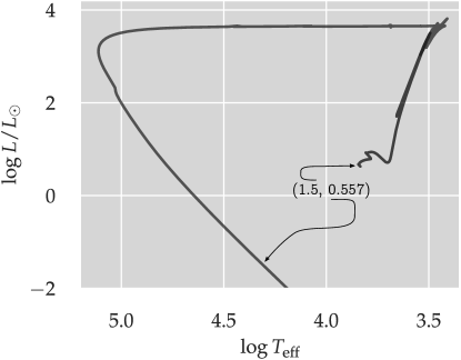
Figure 1: The evolutionary track from the ZAMS to advanced WD cooling of the $M_{\mathrm{ZAMS}}=1.5\,M_{\odot}$ model star that ended as a $0.557\,M_{\odot}$ DA white dwarf. In this report, initial and final masses are coded by tuples as used in the figure.

The mass-loss prescriptions adopted in the evolution computations boil down to quantifying the parameters that measure the strength of a Reimers- and a Blöcker-type mass-loss recipe (cf. Paxton et al., 2011). Initially, the canonical choices Reimers_scaling_factor = 0.1 and Blocker_scaling_factor = 0.2 were used to follow the stars’ evolution as far as possible past the tip of the AGB.

For easier restarts of evolutionary advanced sequences, a breakpoint was set in the computations at around the onset of the ThP-cycles. Additional model sequences (assuming hence the same $M_{\mathrm{ZAMS}}$) could be restarted at these breakpoint-epochs with different choices of the Blocker_scaling_factor. Varying the mass-loss efficiency caused the model stars to leave the AGB after having lived through a different number of ThP cycles, arriving hence at different final masses and also leaving the AGB at different phases within a ThP cycle. With respect to forcing stars off the AGB at different evolutionary stages, this approach reminds of fishing in muddy waters, which it actually is. Nonetheless, the outcome proofed sufficiently useful for this exploratory study.

Forcing the model stars to leave the AGB after different numbers of ThP cycles produced varying proto-WD masses. Leaving the AGB at different phases in their ThP cycles meant that they started departing the AGB at different luminosities and effective temperatures and hence had different $L/M$ ratios. It is important to emphasize that varying the Blocker_scaling_factor is not physically motivated; it is just a convenient numerical dial to turn to enforce departure from the AGB at will to observe the effect it has on the stability of the model stars.

Figure 1 shows the evolutionary track on the HR plane of an $M_{\mathrm{ZAMS}}=1.5\,M_{\odot}$ star model with an initially homogeneous ZAMS $X=0.7,Z=0.02$ composition. As the model evolved up the AGB, it passed through four ThP cycles before the remaining envelope mass got too thin and the star terminated its ascent. The model left the AGB with a remaining mass of $0.557\,M_{\odot}$. The essentially horizontal post-AGB locus shows some minor hiccups but otherwise quietly enters the terminal WD cooling phase. The apparent noise along the almost horizontal post-AGB track are, at closer examination, not signs of poor convergence of the models. Rather, they are phases in which small oscillations develop, but which quickly subside again.

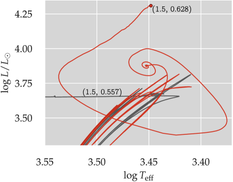
Figure 2: Zoom-in to the top of the AGB. The black locus is the same $1.5\,M_{\odot},Z=0.02$ track as shown in Fig. 1. Superimposed in red is the track from the $(1.5,0.628)$ sequence that was subjected to a different Blöcker-type mass-loss rate during its thermally pulsing AGB phase.

Very late during the AGB evolution, once the model stars’ envelopes get thin enough to initiate the evolution away from the AGB, pulsations with large growth rates were found to develop under favorable circumstances. Figure 2 illustrates how this looks like in the case of the $(1.5,0.628)$ sequence for which, after seven ThP cycles, a high-luminosity departure from the AGB was found for the Blocker_scaling_factor = 0.2 choice. The rapidly growing spiral traces the pulsational instability on the HR plane. Facing such an instability, the evolutionary computations were found to terminate either due to too short timesteps or failing convergence of MESA once the amplitude of the pulsation grows too large (the termination epoch is marked by the red dot in Fig. 2). The pulsationally stable $(1.5,0.557)$ sequence (grey locus) was computed with Blocker_scaling_factor = 0.4. As mentioned before, the respective star evolved through four ThP cycles before it left the AGB to transit to the WD cooling branch without any signs of an unfolding oscillatory instability.

3.1. THE PULSATIONAL INSTABILITY

To gather experience on the frequency of the occurrence of pulsations of the kind stumbled over in the $M_{\mathrm{ZAMS}}=1.5\,M_{\odot}$ case reported in the last section, additional model sequences were computed with different choices of Blocker_scaling_factor in the hope of discovering further cases that develop pulsations.

Table 1: $Z=0.02$ model sequences that developed pulsations. The pulsations of the highlighted row are representative and discussed vicariously in the text.

($M_{\mathrm{ZAMS}},M_{\mathrm{final}}$) in s.u.	$\log L/L_{\odot}$	P / d	$\#$ of puls. cycles	Blocker_scaling_factor
(1.5, 0.628)	3.87	1004	3	0.2
(1.8, 0.605)	3.80	436	7	0.1
(2.0, 0.570)	3.74	98	11	0.4
(2.0, 0.650)	3.85	779	3	0.1
(3.0, 0.781)	3.97	1288	3	0.1
(3.0, 0.641)	3.86	719	4	1.0

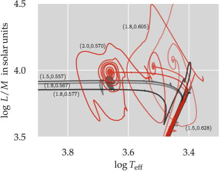
Figure 3: Selected evolutionary tracks of the PopI ($Z=0.02$) model sequences on the $T_{\rm eff}-L/M$ plane hint at tracks reaching sufficiently large $L/M$ ratios to be prone to pulsations.

Table 1 collects useful properties of those model sequences, characterized by the respective (initial-,final-mass) tuples in the first column, that developed radial pulsations at the end of their AGB evolution. The magnitude of the only parameter that was changed in the inlist for a given initial mass, Blocker_scaling_factor, is listed in column five. The number of pulsation cycles that could be followed with MESA before it stalled is collected in the fourth column. Column two lists the luminosity at which the pulsations started to grow. The third column finally contains the pulsation period in days, derived as the average over the computable pulsation cycles.

Columns two and three of Table 1 reveal that the pulsation period and the star’s luminosity are correlated. The brighter the star, the longer is the period. Mapping the data from the table onto the $PL$-relations in Trabucchi et al. (2019) shows, however, that the results reported here do not match a single branch of their relations. Compared with LPV pulsations discussed in the literature, the pulsations from Table 1 are generally overluminous at a given period.

As it is evident from Table 1, pulsations develop in all sequences with $M_{\mathrm{ZAMS}}>1.5M_{\odot}$. None of the mass-loss choices adopted in the $M_{\mathrm{ZAMS}}=1.1M_{\odot}$ case allowed the model stars to pulsate around the termination of their AGB evolution. Evidently, the higher the starting mass of the model stars is, the easier it seems for them to pick up rapidly-growing pulsations. The collection of evolutionary tracks devoid of pulsations (grey) and respective ones (i.e. same $M_{\mathrm{ZAMS}}$) with terminal pulsations (red) on the $\log T_{\rm eff}-\log L/M$ plane of Fig. 3 hints at the $L/M$ ratio to have to exceed a critical level for pulsations to develop. To keep Fig. 3 reasonably readable, only tracks of $1.5,1.8,$ and $2.0\,M_{\odot}$ sequences are included.

The horizontal post-AGB tracks of the stable (grey) evolutionary sequences in Fig. 3 all display a few noisy phases, some even with non-negligible amplitudes (such as along (1.5, 0.557) and (1.8, 0.567) tracks). Such fidgeting is not a sign of numerical convergence problems. Closer inspection of the larger-amplitude wiggles shows that these are associated with phases of small-amplitude pulsations that failed to overcome the first growth regime. The iterative process to compute a model star usually generates structural perturbations that may serve as seeds for such instabilities to grow. Along the grey loci, perturbations can apparently persist for a short while but eventually they damp out again. In contrast, along the red evolutionary tracks, pulsations unfold with large growth rates so that they reach the nonlinear regime within a few pulsation cycles.

3.2. POPULATION II STARS

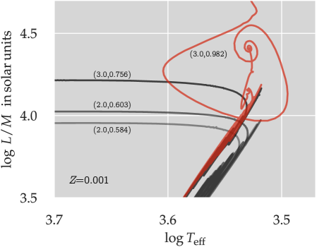
Figure 4: The red locus traces on the $\log T_{\rm eff}-\log L/M$ plane the final AGB evolution and the pulsation encountered in the (3.0,0.982) PopII sequence. The stable evolutionary tracks of the $M_{\mathrm{ZAMS}}=2.0$ and $3.0\,M_{\odot}$ choices are plotted in grey.

The results presented in Sect. 3.1 are appropriate for PopI-like stars only. In the astrophysical context of AGB evolution, the behavior of more metal-poor stars is relevant and pulsations are usually sensitive to the chemical composition of the stellar matter. Hence, additional model sequences were computed that started with a PopII-like homogeneous ZAMS composition of $X=0.758,Z=0.001$. Metal-poor stars are known to be bluer than their brethren with higher heavy-element abundances. The PopII evolutionary tracks up the AGB are comparatively hotter, and the configurations are therefore more compact than respective PopI model stars.

As Table 2 – the table-of-one-row – already hints at, in PopII stars early – post-AGB pulsations are harder to find than in PopI models. In case of the adopted PopII-like composition, stars with $M_{\mathrm{ZAMS}}\lesssim 3\,M_{\odot}$ fail to develop the sought pulsations. Currently, only one case can be reported: The $(3.0,0.982)$ sequence displayed on the $\log T_{\rm eff}-\log L/M$ plane of Fig. 4. The model departed from the AGB at around $\log L/L_{\odot}=4.4$, which is considerably higher than what is seen in respective PopI sequences. The pulsation period, averaged over the three computable cycles, was accordingly long with $1097$ days. The motivation to choose a low value of the Blöcker-type mass-loss was to force to star to stay longer, i.e. to live through more ThPs that take it further up along the AGB with each cycle. The $16$ pulses the $(3.0,0.982)$ sequence went through were eventually enough to build up a sufficiently tenuous outer envelope in which a pulsation developed. Figure 4 suggests that, compared with the $Z=0.02$ sequences, PopII stars require a larger $L/M$ ratio to host pulsations.

Table 2: The $Z=0.001$ model sequence that developed a terminal pulsation.

($M_{\mathrm{ZAMS}},M_{\mathrm{final}}$) in s.u.	$\log L/L_{\odot}$	P / d	$\#$ of puls. cycles	Blocker_scaling_factor
(3.0, 0.982)	4.4	1097	3	0.05

To reach sufficiently high $L/M$ ratios for pulsations to unfold, the lowest-mass model sequences, $(1.5,0.628)$ for PopI and $(3.0,0.982)$ for PopII composition, had both to be in the phase of a He-shell flash. Hence, at the low-mass end, the chances for pulsations to occur are low because the respective AGB star must be in the proper, comparatively short-lived phase of the ThP cycle during which the He-shell is thermally unstable. Going up in mass, pulsations can however develop essentially at any phase through a ThP cycle. In the higher-mass PopI model sequences computed in this study, the H- and He-shell were both active, with the H-shell being the dominant energy source, when the pulsations developed.

4. THE NATURE OF THE PULSATIONS

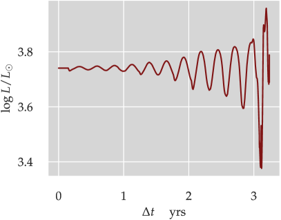
Figure 5: The temporal growth of the luminosity variation during the terminal pulsational instability of the $(2.0,0.570)$ sequence.

This section focuses on the pulsation that develops in the PopI $(2.0,0.570)$ sequence. It is the one whose terminal pulsation period is comparatively short with about $98$ days. The astrophysical variability behavior is nonetheless representative, it does not differ much from the longer-period pulsations of the sample presented here. The relatively large number of pulsation cycles that could be followed numerically invite some standard diagnostics from classical pulsation theory to be applied.

Figure 5 illustrates the rapid growth of the amplitude of the cyclic luminosity variation; the zero-point of the abscissa was chosen arbitrarily around the onset of the variability. Apparently, the pulsation does not grow out of computational noise but gets initiated by a small but finite amplitude-kick, which is likely picked up during the numerical relaxation process.

The pulsational radial velocity ($v_{\mathrm{puls}}$) of the star’s surface (Fig. 6) visualizes once again the rapid growth of the pulsation; the nonlinearity is well expressed after about six pulsation cycles. This development goes in par with the bolometric light change displayed in Fig. 5. The comparison of $v_{\mathrm{puls}}$ with the escape velocity from the surface ($v_{\mathrm{esc}}$) explains why MESA eventually fails to converge or stalls once the outermost layers approach escape velocity. It is a common feature of all the pulsating model sequences in Table 1 that their photospheric pulsation velocity approach escape velocity at the end of the simulation runs.

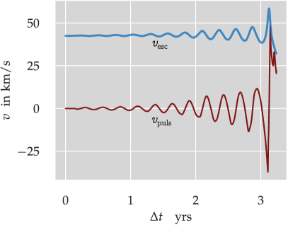
Figure 6: After less than a dozen pulsation cycles the pulsational radial velocity at the surface approaches escape speed.

The pulsational instability depicted in Figs. 5 and 6 gives the impression that it grows exponentially. This is indeed the case as can be directly deduced from a plot of the temporal evolution of the model star’s directed kinetic energy. The appropriate quantity, $E_{\mathrm{kin}}$, is plotted in Fig. 7 on a logarithmic scale. A decently matching linear fit to $E_{\mathrm{kin}}(\Delta t)$ yields an e-folding time of about 140 days. This means that the kinetic energy grows by a factor e in less than two pulsation cycles. According to Fig. 7, the directed kinetic energy starts at around $5\cdot 10^{38}$ erg and quickly grows to about $6\cdot 10^{42}$ erg. Within less than a dozen cycles, $E_{\mathrm{kin}}$ grows by about four orders of magnitude. Nonetheless, the total (potential and internal) energy of the star is of the order of $-10^{49}$ erg. Hence, the kinetic energy of the pulsation remains, even at maximum amplitude, a minor contribution to the energy budget of the star. From the energetic point of view, the initial growth of the coherent pulsational motion with its $5\cdot 10^{38}$ erg is – numerically seen – still developing out of the noise.

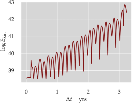
Figure 7: On a logarithmic scale, the growth of the star’s kinetic energy (measured in erg) is essentially linear.

The temporal variation over the almost 12 pulsation cycles of the photospheric radius (red) and radii of selected mass levels close to the star’s surface are assembled in Fig. 8. The deepest-lying mass level that is plotted lies at $\log(1-m/M_{\ast})=-3.0$; i.e. only the outermost about $10^{-3}$ of the star’s mass is contained in the plot. The various mass shells were chosen purely for illustrative purposes. To quantify the unusual behavior of the mass layers in the plot, two more of them are labeled numerically.

The $\log(1-m/M_{\ast})=-3.0$ mass-level is hardly affected by the pulsation. Even though it shows some cyclic modulation it contracts monotonically as does the majority of the star already. The mass-level tagged with $-3.10$ participates in the pulsation almost to the end of the simulation but eventually joins the contraction of the rest of the model star. Mass-layers above the $-3.12$ level, on the other hand, constitute a very thin envelope that oscillates to the very end of the computation and whose compression- and expansion-kinematics hints at the formation of shock fronts during contraction. The picture that emerges from Fig. 8 is that of a mostly contracting interior plus a thin pulsating outer envelope that evolves towards detachment on a time-scale of years or less. These two regions clamp a low-density cavitation-like layer that induces temporarily pronounced density inversions at its outer edge.

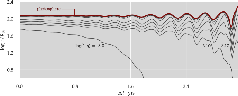
Figure 8: Temporal radius variation of selected mass shells close to the star’s photosphere. Only the very outermost layers participate in the cyclic variability.

During cycle 10, the second to the last cycle shown in Fig. 8, the amplitudes of the pulsation-induced variations in the outer envelope are considerable and nonlinearities are already well developed. Figure 9 illustrates from a complementary angle the relative radius variability contained in Fig. 8.

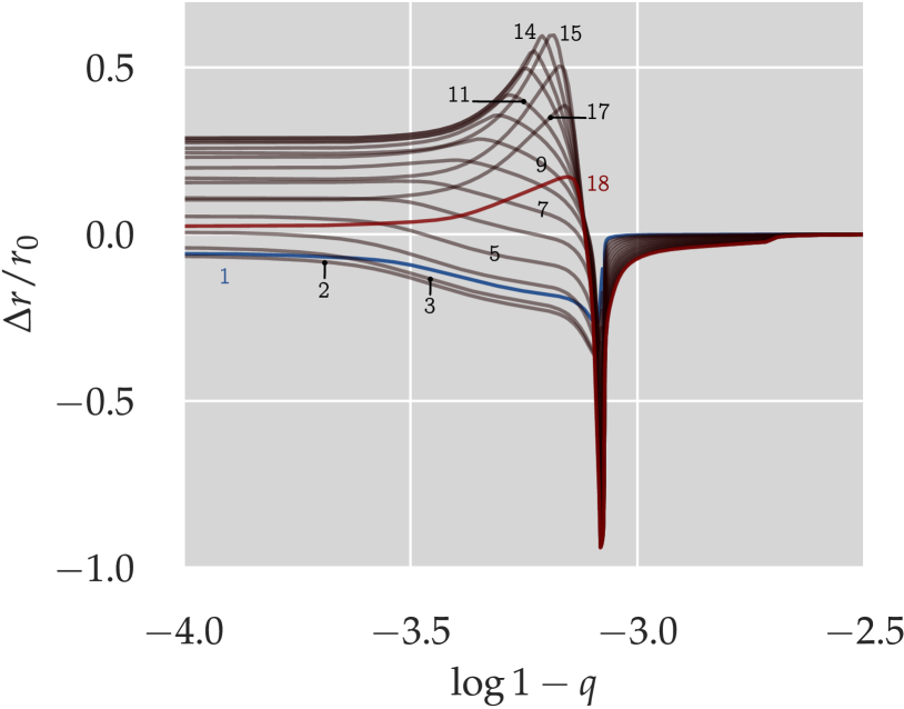
Figure 9: Relative radius-variation profiles at 18 epochs during pulsation-cycle 10.

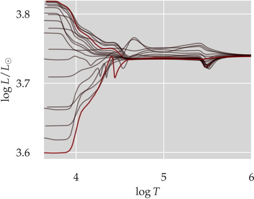
Figure 10: At the same phases as in Fig. 9, a collection of luminosity profiles.

MESA computed 18 epochs to cover pulsation-cycle 10. The arbitrary chosen epoch 0 serves as the reference profile relative to which the quantity $\Delta r/r_{0}\equiv(r-r_{0})/r_{0}$ is calculated. To help to read the progression of the relative radius change over a pulsation cycle the profiles in Fig. 9 are numbered. The first epoch is additionally colored in blue, the last epoch of the chosen cycle is plotted in red. This coloring helps to emphasize the temporal radius behavior in the region $\log(1-q)\gtrsim-3.1$: As pointed out in Fig. 8 already, these deeper layers do not participate in the oscillatory motion but only shrink monotonously. The contraction magnitude decreases with mass depth and vanishes before the outer edge of the H-burning shell is reached. All in all, the relative radius-variation over a cycle of our pulsating early – post-AGB stars does not resemble the eigenfunctions one is used to from classical pulsators.

The variation of the spatial luminosity profiles over pulsation cycle 10 is a further illustration of how different the pulsations of the early – post-AGB stars are from classical pulsators. In accordance with Fig. 8, the pulsation affects only the regions cooler than $10^{6}$ K. Between the $Z$-bump and the He⁺-partial ionization zone ($\log T\approx 4.5$), on the average the luminosity rises only; i.e. it is not an oscillation about a quasi-equilibrium configuration. This changes in regions closer to the photosphere, there the luminosity varies such that it falls below the luminosity prevailing in the pulsation-unaffected depth of the star ($\log T\gtrsim 6$) at some phases and exceeds that luminosity about half a cycle later. Except for the regions with $\log T\lesssim 4.5$, the spatial variability is unlike the harmonic behavior seen in the common pulsating stars. To emphasize the peculiarity of the variability profiles, maximum and minimum light phases are highlighted in red in Fig. 10.

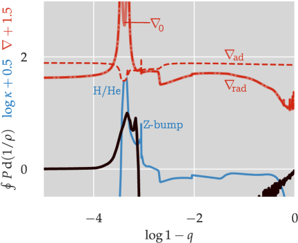
Figure 11: Differential work over a pulsation cycle (black) and the spatial run of the vertically shifted Rosseland opacity of the first model of the cycle (blue) to help to identify the source of pulsation driving.

None of the pulsations discussed here could ever be tracked to saturation, i.e. they never reached strict periodicity. Nonetheless, driving and damping regions in the envelopes were tried to be identified by computing the differential work integral

$$\Delta W=\oint\displaylimits_{\mathrm{cylce}}\!P\,{\mathrm{d}}_{t}\Delta V{\mathrm{d}}t\propto\oint\displaylimits_{\mathrm{cylce}}\!P\,{\mathrm{d}}\left(\frac{1}{\rho}\right)\,,$$

per mass shell $\Delta m$ over a pulsation cycle. The differential work integrals were computed during the still rather smooth cycles 8 and 9. Different initial phases, from which a quasi-cycle was defined, were tried out. The results all looked like what is plotted in Fig. 11, where the differential work is arbitrarily normalized to maximum driving. Even though the details of the driving region ($\Delta W>0$) varied depending on the starting phases of a cycle, the driving and damping region remained spatially stable, independent of the particular numerical choices. To correlate the driving region with envelope properties, Fig. 11 shows also the vertically shifted Rosseland-opacity profile of the starting model of the cycle. All the pulsation driving is confined to the partial ionization-region of H/He. At the base of the $Z$-bump, the pulsation is already strongly damped. The damping computed in the even deeper, i.e. hotter layers becomes eventually useless because the respective mass shells do not participate in the cyclic pulsation; they undergo purely monotonous state changes only (cf. Fig. 8) so that the path integral along a cycle has no basis anymore. The important take-away is that driving occurs in the partial ionization-regions of H and He. These regions coincide with the large-amplitude, also spatially pulsational variability seen in the profiles of the model stars.

We finish with the successful recovering the pulsations also in the QHE ansatz. A few cases only were computed so far. Particularly interesting are the $M_{\mathrm{ZAMS}}=2\,M_{\odot}$ cases: There, the QHE and dynamical evolution computations behave identical, as exemplified by the (2.0, 0.570) sequence shown in Figure 12 where the terminal evolutionary tracks on the AGB and the departure therefrom are mapped onto the HR plane. The result of the dynamical treatment is traced out by the red line. The broader grey line shows the evolution of the same model star in QHE mode. Even the small bumps along the evolutionary tracks are identical. The two $2\,M_{\odot}$ cases are important counterexamples to the interpretation of the pulsations presented here as radial acoustic modes. Thanks to the pulsations persisting also in the QHE approximation it is clear that these pulsations are not excited acoustic waves as known from classical pulsators. Furthermore, the dynamical treatment of the evolution problem does not lead to a more dynamic or even monotonic instability.

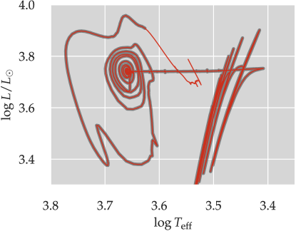
Figure 12: Terminal evolution along the AGB of the (2.0, 0.570) sequence, once computed dynamical (red) and once in QHE (thick grey line).

Under the physical conditions prevailing in the envelopes of very luminous AGB stars, thermal and dynamical timescales become comparable and the distinction between acoustic and thermal modes gets ever more difficult to maintain. It has been known for a long time (e.g. Wood, 1976; Gautschy & Glatzel, 1990; Saio et al., 1998) that strange modes that have no counterparts in the adiabatic acoustic mode-spectrum of a star might develop around $L/M\sim\mathcal{O}(10^{4})$ with pulsation periods that can exceed those of the fundamental radial p-mode. Such modes can go unstable with very large growth rates. These properties are all features which also fit in the pulsational instability encountered in the early – post-AGB model stars.

5. WRAPPING IT ALL UP

Lagrangian, dynamical MESA evolution computations revealed, under suitably favorable conditions, the development of rapidly growing radial pulsations shortly after or around the termination of the AGB evolution of initially low- and intermediate mass stars. The periods found range from about 100 to over 1000 days. The e-folding times of a few periods’ length are much shorter than what is encountered in classical pulsators. The behavior is reminiscent of the pulsations of massive red-supergiants (e.g. Yoon & Cantiello, 2010) that were also successfully tracked with MESA (Paxton et al., 2013). With the model sequences discussed in this proof-of-concept report, dynamical MESA computations demonstrate that they are capable of recovering oscillatory instabilities at the end of AGB evolution of low-mass stars as reported by Wagenhuber & Weiss (1994). The latter authors found such pulsations in their QHE computations confined to around maximum instability of the models’ He-shell. Within a few years of a star’s evolution time, i.e. after only a few pulsation cycles the model stars build up superficial radial pulsation velocities that approach escape speed. Eventually, convergence of the models failed due to the constraints of the numerical approach to evolve these stars.

In two MESA model sequence so far, the QHE and the dynamical evolution of the model stars are found to behave identical. Hence, this step beyond what Wagenhuber & Weiss (1994) found does not substantiate their expectation that the instability seen in their QHE treatment would turn into a dynamical instability. It is rather more obvious to understand these pulsations as thermal strange modes, seen directly in their nonlinear regime.

The pulsations are found to develop in a very thin – $\mathcal{O}(\lesssim 10^{-3}\,M_{\odot})$ – surface layer whose oscillation amplitude grows rapidly on top of a monotonously shrinking interior. Between these two regions a low-density cavitation-like region (cf. Fig. 8) builds up. At the low densities and the strong radiation fields that prevail in the outermost layers of the pulsating post-AGB stars, matter and radiation are likely out of equilibrium so that a radiation-hydrodynamic treatment of the problem is called for. More appropriate computational tools that can follow the dynamics also across the transition from the stellar surface into the circumstellar medium must scrutinize the pulsations found in the MESA computations. It will be interesting to learn if the pulsations persist and if they do, what the dynamics of the density-inversion region (the cavitation) is, and how much mass the pulsation is able to shed.

Even in the coolest early – post-AGB pulsators (e.g. Fig. 3) the envelope convection zones are shallow. Mostly, the regions around the opacity $Z$-bump and the H/He partial ionization zones are convectively unstable. The way mixing-length convection is treated in stellar evolution computations means that convection adapts instantaneously to the local physical states through the star. The encountered pulsation periods of hundreds of days are, however, not that different from the convection timescale. Figure 11 shows representatively (in red) the pertinent temperature gradients in early – post-AGB pulsators. The dashed line traces $\nabla_{\mathrm{ad}}$, $\nabla_{\mathrm{rad}}$ is shown as a dot-dashed line, which is mostly covered by the thicker, transparent full line of $\nabla_{0}$, the effectively prevailing temperature gradient. The very thin (in mass) convection zone at the $Z$-bump is still adiabatic. In contrast, the convection region around H/He partial ionization, where pulsation driving occurs, is very non-adiabatic. Hence, only a fraction of the total flux is effectively transported by material motion in the driving region. As it was already called for by Wagenhuber & Weiss (1994) under comparable circumstances, the effect of time-dependent convection on the instability needs to be investigated. Such an endeavor should be feasible now after the local, time-dependent convection formalism of Kuhfuß was added to MESA’s toolbox (Jermyn et al., 2023).

Based on the presented results, early – Post-AGB pulsations can emerge over a broad range of phases of a ThP cycle. The rapid growth of the instability has the potential to shed much of the superficial layers – of the order of $10^{-4}-10^{-3}\,M_{\odot}$ – within a few years. It should be interesting to learn what fraction of the observed $25\%$ H-poor central stars of planetary nebulae could be produced by first-time descendants from the AGB already, i.e. by pulsating early – post-AGB stars. If this is possible, this should induce a mass-dependent signature. For lower-$M_{\mathrm{ZAMS}}$ stars to develop pulsations a He-shell instability seems to be necessary . Hence, this scenario would naturally satisfy the requirement of a correlation of mass-loss and thermal-pulse cycle (Blöcker, 2001). Higher initial masses, on the other hand, are seen to leave the AGB and develop pulsations almost at any phase during the ThP cycle. Furthermore, a metallicity dependence is to be expected too. Metal-poorer stars were found to develop early – post-AGB pulsations for comparatively higher $M_{\mathrm{ZAMS}}$ only.

Post-AGB stars that live through a (very) late thermal pulse (Blöcker, 2001) can return to the AGB as so-called born-again AGB stars and reach thereby sufficiently high luminosities and low effective temperatures to (possibly once again) develop pulsations of the kind presented in this study. The peculiar variable stars FG Sge (Jurcsik & Montesinos, 1999), V 605 Aql, and Sakurai’s object (Lawlor & MacDonald, 2002) might be examples of or candidates for such objects. During such a very late phase of recurring dynamical mass-loss, any remaining thin H-rich envelope might become either very depleted or even get completely lost.

This report raises more questions than it answers. Nevertheless, a selfconsistent mechanism – computationally established with complete stellar-evolution models – is reiterated on to argue that it might serve as the physical machinery that drives the hitherto hypothetical superwind. The preliminary results computed with MESA hint at several promising and potentially rewarding research avenues in the field of AGB and post-AGB stellar astrophysics that should be accessible now to the available computational tools.

ACKNOWLEDGEMENTS: This work relied substantially on NASA’s Astrophysics Data System. The model stars were computed with the MESA  software-instrument, version r$21.12.1$ (Paxton et al., 2019). Postprocessing MESAstar models and plotting benefited from Warrick Ball’s tomso, numpy (Harris et al., 2020), scipy (Virtanen et al., 2020), and matplotlib (Hunter, 2007), respectively. I am profoundly grateful to have had free access to all these software tools and to the full texts of much of the cited scientific literature.

APPENDIX

&star_job
      !...Nuclear physics
      change_net    = .true.
      new_net_name  = ’approx21.net’

      ! Macrophysics part
      change_v_flag = .true.
      new_v_flag    = .true.
/ !end of star_job namelist

&eos
     ! eos options
     ! see eos/defaults/eos.defaults
/ ! end of eos namelist

&kap
      kap_file_prefix      = ’a09’
      kap_lowT_prefix      = ’lowT_fa05_a09p’
      kap_CO_prefix        = ’a09_co’
      use_Type2_opacities  = .true.
      Zbase                = 0.02d0
/ ! end of kap namelist

&controls
      !...to start evolution from ZAMS
      initial_mass = 1.5d0
      initial_z    = 0.02d0

      energy_eqn_option   = ’dedt’
      use_gold_tolerances = .true.

      !...Convection
      mixing_length_alpha = 1.8d0
      MLT_option          = ’Cox’

      use_Ledoux_criterion  = .false.
      do_conv_premix        = .false.

      !...Overshooting
      overshoot_scheme(1)    = ’exponential’
      overshoot_zone_type(1) = ’burn_H’
      overshoot_zone_loc(1)  = ’core’
      overshoot_bdy_loc(1)   = ’top’
      overshoot_f(1)         = 0.012
      overshoot_f0(1)        = 0.002

      overshoot_scheme(2)    = ’exponential’
      overshoot_zone_type(2) = ’nonburn’
      overshoot_zone_loc(2)  = ’shell’
      overshoot_bdy_loc(2)   = ’bottom’
      overshoot_f(2)         = 0.022
      overshoot_f0(2)        = 0.002

      make_gradr_sticky_in_solver_iters = .true.

      !...Mass-loss processes
      cool_wind_RGB_scheme   = ’Reimers’
      Reimers_scaling_factor = 0.1
      cool_wind_AGB_scheme   = ’Blocker’
      Blocker_scaling_factor = 0.2
      RGB_to_AGB_wind_switch = 1d-4   Ψ

      !...time-step & grid control
      delta_HR_limit    = 0.02

/ ! end of controls namelist

References

- Blöcker (1995) Blöcker, T. 1995, A&A, 297, 727
- Blöcker (2001) Blöcker, T. 2001, Ap&SS, 275, 1
- Decin (2021) Decin, L. 2021, ARAA, 59, 337
- Freytag & Höfner (2023) Freytag, B. & Höfner, S. 2023, A&A, 669, A155
- Gautschy & Glatzel (1990) Gautschy, A. & Glatzel, W. 1990, MNRAS, 245, 597
- Harris et al. (2020) Harris, C. R., Millman, K. J., van der Walt, S. J., et al. 2020, Nature, 585, 357
- Herwig (2005) Herwig, F. 2005, ARAA, 43, 435
- Hunter (2007) Hunter, J. 2007, CSE, 9, 90
- Jermyn et al. (2023) Jermyn, A. S., Bauer, E. B., Schwab, J., et al. 2023, ApJS, 265, 15
- Jurcsik & Montesinos (1999) Jurcsik, J. & Montesinos, B. 1999, NewAR, 43, 415
- Karakas & Lattanzio (2014) Karakas, A. I. & Lattanzio, J. C. 2014, PASA, 31, e030
- Lawlor & MacDonald (2002) Lawlor, T. M. & MacDonald, J. 2002, in ASP Conf. Ser., Vol. 279, Exotic Stars as Challenges to Evolution, IAU Coll. 187, ed. C. A. Tout & W. V. Hamme, 193
- Paxton et al. (2011) Paxton, B., Bildsten, L., Dotter, A., et al. 2011, ApJS, 192, 3
- Paxton et al. (2013) Paxton, B., Cantiello, M., Arras, P., et al. 2013, ApJS, 208, 4
- Paxton et al. (2019) Paxton, B., Smolec, R., Schwab, J., et al. 2019, ApJS, 243, 10
- Reimers (1975) Reimers, D. 1975, in Problems in Stellar Atmospheres and Envelopes, ed. B. Baschek, W. H. Kegel, & G. Traving (Springer Verlag), 229
- Renzini (1981) Renzini, A. 1981, in ASSL, Vol. 88, Physical Processes in Red Giants, 431
- Saio et al. (1998) Saio, H., Baker, N., & Gautschy, A. 1998, MNRAS, 294, 622
- Trabucchi et al. (2019) Trabucchi, M., Wood, P. R., Montalbán, J., et al. 2019, MNRAS, 482, 929
- Van Winckel (2003) Van Winckel, H. 2003, ARAA, 41, 391
- Virtanen et al. (2020) Virtanen, P., Gommers, R., Oliphant, T. E., et al. 2020, Nature Methods, 17, 261
- Wagenhuber & Weiss (1994) Wagenhuber, J. & Weiss, A. 1994, A&A, 290, 807
- Wood (1976) Wood, P. R. 1976, MNRAS, 174, 531
- Wood (1981) Wood, P. R. 1981, in ASSL, Vol. 88, Physical Processes in Red Giants, 205
- Yoon & Cantiello (2010) Yoon, S.-C. & Cantiello, M. 2010, ApJ, 717, L62