A Bayesian Approach To The Halo-Galaxy-SMBH Connection Through Cosmic Time

Abstract

Aims. We study the co-evolution of dark matter halos, galaxies and supermassive black holes using an empirical galaxy evolution model from $z=0$ – $10$. We demonstrate that by connecting dark matter structure evolution with simple empirical prescriptions for baryonic processes, we are able to faithfully reproduce key observations in the relation between galaxies and their supermassive black holes.

Methods. By assuming a physically-motivated, direct relationship between the galaxy and supermassive black hole properties to the mass of their host halo, we construct expressions for the galaxy stellar mass function, galaxy UV luminosity function, active black hole mass function and quasar bolometric luminosity function. We calibrate the baryonic prescriptions using a fully Bayesian approach in order to reproduce observed population statistics. The obtained parametrizations are then used to study the relation between galaxy and black hole properties, as well as their evolution with redshift.

Results. The galaxy stellar mass – UV luminosity relation, black hole mass – stellar mass relation, black hole mass – AGN luminosity relation, and redshift evolution of these quantities obtained from the model are qualitatively consistent with observations. Based on these results, we present upper limits on the expected number of sources for $z=5$ up to $z=15$ for scheduled JWST and Euclid surveys, thus showcasing that empirical models can offer qualitative as well as quantitative prediction in a fast, easy and flexible manner that complements more computationally expensive approaches.

1 Introduction

The scaffolding of galaxy formation and evolution is provided by the distribution of dark matter in the Universe. It is well established that galaxies form and grow within gravitationally bound dark matter halos, leading to tight correlations between the properties of galaxies and their host halos (e.g. Fall & Efstathiou, 1980; Efstathiou & Silk, 1983; Blumenthal et al., 1984; Wechsler & Tinker, 2018).

In standard Lambda Cold Dark Matter ($\Lambda$CDM) cosmology, the growth of dark matter halos is thought to occur hierarchically (Peebles, 1965; Silk, 1968; White & Rees, 1978), with steady accretion of intergalactic matter and merging of gravitationally bound halos playing significant roles (e.g. Toomre & Toomre, 1972; White & Rees, 1978; Barnes, 1988). Since the behaviour of dark matter on large scales is governed solely by gravity, dark matter structure formation is generally considered a well-understood process supported by analytical and numerical models (Press & Schechter, 1974; Sheth et al., 2001; Despali et al., 2015). The evolution of galaxies within these halos on the other hand, is a more complex process, involving a large variety of baryonic processes across all scales regulating galaxy growth. The gravitational evolution of galaxies is dominated by the much more massive halos they inhabit, but simultaneously, non-gravitational interactions such as radiative cooling, stellar evolution, and feedback from stars and active galactic nuclei (AGN) add an additional layer of complexity (e.g. Dekel et al., 1986; White & Frenk, 1991; Naab & Ostriker, 2017). An area of particular interest is the connection between galaxies and their central supermassive black holes (SMBHs), as research has revealed they have properties that are closely related (Gebhardt et al., 2000; Ferrarese & Merritt, 2000; Davis et al., 2017), suggesting their evolution to be tightly interconnected. The existence of a near-linear relationship between star-formation rate and stellar mass, known as the galaxy main sequence, suggests that these baryonic processes play a major role in regulating galaxy growth and star formation (Brinchmann et al., 2004; Whitaker et al., 2014; Tomczak et al., 2014; Popesso et al., 2019; Sherman et al., 2021; Lilly et al., 2013). In order to gain a comprehensive understanding of galaxy evolution, it is therefore necessary to study the evolution of dark matter, galaxies, and black holes in conjunction.

Star formation and active galactic nuclei (AGN) powered by accretion onto the central SMBH are principal contributors to gas heating and outflows in galaxies. Stars inject a considerable amount of energy and momentum into the interstellar medium through stellar winds, electromagnetic radiation and supernovae. These processes heat or directly eject gas from the galaxy, thereby depleting it of fuel for further star formation (e.g. Larson, 1974a, b; Dekel et al., 1986; Hopkins et al., 2012). At the same time, the accretion of matter onto SMBHs at the center of galaxies releases enormous amounts of energy and momentum into its surrounding, which heats and eject the nearby gas, similarly affecting star formation (Silk & Rees, 1998; Croton et al., 2006). Dekel et al. (1986) have shown that stellar feedback can be an effective mechanism for removing gas from low mass galaxies as the gas within is less tightly bound to the parent galaxy, while Silk & Rees (1998) have argued that AGN feedback is more effective in removing gas from massive galaxies, while its role in dwarf galaxies is still uncertain (Dashyan et al., 2018; Koudmani et al., 2019, 2021, 2022; Trebitsch et al., 2018; Sharma et al., 2020). These arguments are largely in agreement with observational studies on the stellar mass – halo mass relation (e.g. Guo et al., 2010; Moster et al., 2010; Behroozi et al., 2010; Reddick et al., 2013; Moster et al., 2013) and galaxy stellar mass function (e.g. Ilbert et al., 2013; Duncan et al., 2014; Davidzon et al., 2017). Furthermore, Bower et al. (2017) argue that the shutdown of stellar-driven outflows in massive galaxies causes accretion rates onto SMBHs to increase and thus increases the efficiency of AGN feedback. Consequently, it is essential to consider the effects of stellar and AGN feedback concurrently when modeling the evolution of galaxies and SMBHs.

No single model can fully capture all aspects of galaxy evolution, which involves a wide range of physical scales and processes. As a result, a variety of modeling techniques have been developed, each with their own trade-offs between complexity and comprehensiveness. The most commonly used methods are semi-analytical and semi-numerical models that combine numerical simulations of dark matter with analytical prescriptions for baryonic physics (White & Frenk, 1991; Kauffmann et al., 1993; Cole et al., 1994; Somerville & Primack, 1999; Benson et al., 2002; Lacey et al., 2016; Poole et al., 2016) and full hydrodynamical simulations that jointly track the assembly of dark and baryonic matter (Navarro & White, 1994; Vogelsberger et al., 2014; Schaye et al., 2015; Dubois et al., 2016; Nelson et al., 2019). These models have been instrumental in advancing our understanding of galaxies, but they come at the cost of being computationally expensive and time-consuming to run, making it challenging to explore the available parameter space. Additionally, many of the processes involved in galaxy evolution remain below the resolution limit of simulations, and need to be parameterized based on physical or empirical arguments. For these types of models, the prescriptions used are often physics-based, meaning that they are based on fundamental physical processes that lead to specific properties of galaxies that can be compared to observational data.

Empirical models on the other hand, rely on observational relations and conceptual arguments alone to infer physical constraints (White & Frenk, 1991; Rodríguez-Puebla et al., 2016; Sharma & Theuns, 2019). Such models can be fully analytical or merger tree-based, and can include a wide range of physical processes or be be stripped down to key components important for studying a particular question at hand. Examples of such models are EMERGE (Moster et al., 2018), UniverseMachine (Behroozi et al., 2019) and Trinity (Zhang et al., 2022), which are comprehensive empirical models containing around 50 free parameters and datasets of 10 observational constraints, aimed to study the evolution of galaxies, SMBHs, and their connection to halos from $z=0$ – $10$. These models produce detailed results, but they also come with a high computational cost and can be challenging to interpret the impact of individual parameters. On the other hand, the simple model proposed by Salcido et al. (2020), aimed at connection halo and stellar population statistics, has few and easily interpretable parameters but does not include SMBHs and does not account for evolution in baryonic processes.

In this study, we aim to bridge this gap in empirical models of the co-evolution of halos, galaxies, and AGN. We develop a model that connects halos to the properties of galaxies and AGN using simple analytical relations, which are calibrated using observational data on the galaxy stellar mass function (GSMF, $z=0-10$), galaxy UV luminosity function (UVLF, $z=0-10$), active black hole mass function (active BHMF, $z=0-5$) and quasar bolometric luminosity function (QLF, $z=0-7$). This allows us to study the co-evolution of these four quantities over a redshift range of $z=0-10$.

The simplicity of our model makes it easy to interpret the involved parameters and their evolution, and its reduced computational complexity allows us to perform a full Bayesian exploration of parameter space, providing a comprehensive understanding of the scope and limitations of the model, while utilizing all the information in the observational data. We validate our model using independent observational datasets on the relationships between the observables, specifically the galaxy stellar mass – UV luminosity relation, SMBH mass – stellar mass relation, and SMBH mass - AGN bolometric luminosity relation, and make predictions on the expected number densities of galaxies at as-of-yet unobserved redshift that are in good agreement with preliminary JWST Early Data Release results (Donnan et al., 2022; Harikane et al., 2022). This model, being easy to interpret and computationally efficient, can be used to gain a qualitative understanding of galaxy evolution over the observed redshift range and to inform more complex and computationally expensive models in a straightforward manner, as well as make quantitative predictions for upcoming instruments such as Euclid.

The paper is organized as follows: We begin by presenting the theoretical framework of our model, including the assumptions we use to develop analytical relations for the observables in Section 2. In Section 3, we describe the datasets used to calibrate the model, as well as the statistical method employed to match our model to these observations. Validation of the model is covered in Section 4 where we compare the model output against independent datasets on the interrelationship between the observables, and also examine the limitations of the assumptions made. In Section 5, we explore the evolution of our model’s parameters with redshift, and provide predictions for as-of-yet unobserved redshift. Finally, in Section 6, we summarize our findings and provide an overview of the implications and potential applications of our model.

2 Model Description

Our model connects observable baryonic structures and their host halos using empirical relations. We assign properties to galaxies and SMBHs based on the mass of their host halos, in order to reproduce average relations and the evolution of observed quantities with redshift. This approach allows us to probe the relations of observable quantities, detailed in this section. We describe the connection of the number of galaxies and SMBHs to the number density of halos, as well as the parametrization of the physical processes involved. A summary of the model and its parameter can be found in Table 1.

2.1 Connecting Observables To Halo Statistics

The number density of halos at a given redshift is described by the halo mass function (HMF), which can be obtained analytically assuming knowledge about the matter density power spectrum (Press & Schechter, 1974) and is closely matched by results obtained from dark matter assembly simulations. In its analytical form, the HMF is given by

$$\phi(M_{\mathrm{h}})=\diff{n}{\log M_{\mathrm{h}}}(M_{\mathrm{h}},z)=\frac{\overline{\rho}}{M_{\mathrm{h}}}f\left(\nu(M_{\mathrm{h}},z)\right)\left|\diff{\log\nu(M_{\mathrm{h}},z)}{\log M_{\mathrm{h}}}\right|,$$ (1)

where $\bar{\rho}$ is the mean matter density, $\nu$ is the mass variance at a given mass scale and $f$ is called the multiplicity function which depends on the details of the dark matter collapse model (see Appendix A for details). For this work, we use the Sheth–Tormen HMF (Sheth et al., 2001) for ellipsoidal collapse.

To construct our model, we make two simplifying assumptions:

1. The total number $n$ of halos and central galaxies and supermassive black holes in a given cosmic volume are identical, meaning every halo hosts exactly one galaxy and one SMBH (i.e. the occupation fractions $\equiv 1$ across all mass ranges).

2. The observable quantity $q$ in question of the galaxy is, completely determined by an invertible function of the halo mass (but may evolve with redshift), i.e.

   $$q=\mathcal{Q}(M_{\mathrm{h}};z).$$ (2)

The second assumption will not hold true for individual galaxies, which are subject to a wide range of physical mechanisms, but can be understood in a statistical sense when averaged over a large number of objects. For this reason, we expect the model to be able to reproduce average relations between halo mass and observables, but not the scatter in these relations.

Under these two assumptions, the number density of the observables is directly linked to the HMF. For example, given a stellar mass – halo mass relation $M_{\star}=\mathcal{Q}(M_{\mathrm{h}})$, the stellar mass function is given by

$$\phi(M_{\star})=\diff{n}{\log M_{\star}}\left(\mathcal{Q}(M_{\mathrm{h}})\right)=\diff{n}{\log M_{\mathrm{h}}}(M_{\mathrm{h}})\cdot\diff{\log M_{\mathrm{h}}}{\log M_{\star}}\left(\mathcal{Q}(M_{\mathrm{h}})\right)$$ (3)

($\log=\log_{10}$). Thus, the form of Equation 2 fully determines the population statistics of the observables, and by matching this number density to observations we can constrain the quantity – halo mass relation. Further, thanks to the invertibility of Equation 2 we can directly link various observable quantities (see Section 2.4).

Differences in the shape of the HMF and number density of observable properties are attributed to the influence of baryonic processes, including the effects of stellar and AGN feedback, on the formation and evolution of galaxies. We distinguish three feedback regimes (see also Salcido et al., 2020):

• Stellar Feedback Regime: In low mass halos, the star formation injects sufficient amounts of energy into galaxy and efficiently drive gas outflows. This regulates the gas budget of the galaxy and prevents gas build-up in the galactic centre, inhibiting star formation and black hole growth.

• Turnover Regime: In this regime, the mass approaches a critical value at which gravity overcomes the stellar-driven outflows, leading to a build-up of gas in the galaxy, leading to rapid star formation and black hole growth.

• AGN Feedback Regime: In massive halos, black holes grow large enough for AGN to drive effective gas outflows, again regulating gas content and slowing star formation and black hole growth.

Depending on halo mass, galaxies will be dominated by different feedback mechanisms. In order to connect the observed population statistics to the HMF, we need to account for these effects.

Table 1: Summary of modelled population statistics, their parameter and asymptotic behaviour.

Number Density Function	Parameter	Interpretation	Low Mass Slope	High Mass Slope
Galaxy Stellar Mass Function	$A_{\star}$	Average stellar mass – halo mass ratio at $M_{\mathrm{h}}=M_{\mathrm{c}}^{*}$.	$\nicefrac{{\alpha_{\mathrm{HMF}}}}{{(1+\gamma_{\star})}}$	exponential
	$\gamma_{\star}$	Strength of stellar feedback.
	$\delta_{\star}$	Strength of AGN feedback.
	$M_{\mathrm{c}}^{*}$	Turnover (halo) mass for stellar and AGN feedback-dominated regime.
Galaxy UV Luminosity Function	$A_{\mathrm{UV}}$	Average UV luminosity – halo mass ratio at $M_{\mathrm{h}}=M_{\mathrm{c}}$.	$\nicefrac{{\alpha_{\mathrm{HMF}}}}{{(1+\gamma_{\mathrm{UV}})}}$	exponential
	$\gamma_{\mathrm{UV}}$	Strength of stellar feedback.
	$\delta_{\mathrm{UV}}$	Strength of AGN feedback.
	$M_{\mathrm{c}}^{\mathrm{UV}}$	Turnover (halo) mass for stellar and AGN feedback-dominated regime
Black Hole Mass Function	$B$	Average mass of SMBH at $M_{\mathrm{h}}=M_{\mathrm{c}}^{\bullet}$.	$\nicefrac{{\alpha_{\mathrm{HMF}}}}{{\eta}}$	exponential
	$\eta$	Slope of BH mass growth with halo mass for acreeting SMBHs.
	$M_{\mathrm{c}}^{\bullet}$	Critical (halo) mass for SMBH mass model.
Quasar Luminosity Function	$C$	Average bolometric AGN luminosity at $M_{\mathrm{h}}=M_{\mathrm{c}}^{\mathrm{bol}}$ and $\lambda=1$.	$\nicefrac{{\alpha_{\mathrm{HMF}}}}{{\theta}}$	$-\rho$
	$\theta$	Slope of luminosity increase with halo mass for acreeting SMBHs.
	$\lambda_{\mathrm{c}}$	Critical Eddington ratio for power law drop-off of ERDF.
	$\rho$	Slope of ERDF drop-off.
	$M_{\mathrm{c}}^{\mathrm{bol}}$	Critical (halo) mass for AGN luminosity model.

2.2 Star-Forming Galaxies

Figure 1: Demonstration of Feedback Effects on GSMF: Least squares regression of Equation 3 to the observed galaxy stellar mass function at $z=0$ (black dots, see text and Figure 3 for details). The black curve shows the maximum likelihood estimate for a model without feedback ($\gamma_{\star}=\delta_{\star}=0$), i.e. a simple scaling of the HMF; the light grey curve is a stellar feedback-only model ($\gamma_{\star}>0$, $\delta_{\star}=0$), while the purple curve includes stellar and AGN feedback ($\gamma_{\star},\delta_{\star}>0$).

The interplay between stellar and AGN feedback at different halo mass scales leads to a characteristic relation in the stellar mass – halo mass relation. Studies have shown that the galaxy stellar mass function is steeper at the low and high mass end compared to the halo mass function, leading Moster et al. (2010) to propose a double power law relation between halo and stellar mass. This parametrization has been found to closely match the observed relation at $z=0$ obtained from abundance matching, clustering analysis and empirical modelling with an turnover halo mass $M_{\mathrm{c}}\approx 10^{12}M_{\odot}$ (Wechsler & Tinker, 2018). Assuming that feedback processes regulate the rate of star formation, it is reasonable to expect that similar relations will hold for the population of newly formed stars, which are primarily responsible for the UV luminosity of actively star-forming galaxies. We can therefore parameterize Equation 2 the total stellar mass and UV luminosity by

$${\mathcal{Q}}(M_{\mathrm{h}})=A\frac{M_{\mathrm{h}}}{\left(\frac{M_{\mathrm{h}}}{M_{\mathrm{c}}^{\star}}\right)^{-\gamma}+\left(\frac{M_{\mathrm{h}}}{M_{\mathrm{c}}^{\star}}\right)^{\delta}},$$ (4)

where $\mathcal{Q}$ is the stellar mass $M_{\star}$, or UV luminosity $L_{\mathrm{UV}}$, and $A$, $\gamma$, $\delta>0$. In this parameterization, the critical mass $M_{\mathrm{c}}$ indicates the mass scale at which the two feedback processes are of equal strength.

Equation 4 is motivated by the fact that in the low halo mass limit (stellar feedback regime), this function behaves as a power law $q\propto M_{\mathrm{h}}^{1+\gamma}$, while in the high mass limit (AGN feedback regime) we get $q\propto M_{\mathrm{h}}^{1-\delta}$, which resulting in the expected alteration of the halo mass function. For $\delta>1$, the function becomes non-invertible with a maximum at $M_{\mathrm{max}}=M_{\mathrm{c}}\left(\frac{\gamma+1}{\delta-1}\right)^{\frac{1}{\gamma+\delta}}$, meaning parameter space is restricted to $0\leq\delta<1$. To construct the GSMF and UVLF of the observable quantities (stellar mass and UV luminosity) specified by Equation 3, we need the derivative of this function given by

$$\diff{\log q}{\log M_{\mathrm{h}}}(M_{\mathrm{h}})=1-\left[\ \frac{-\gamma\left(\frac{M_{\mathrm{h}}}{M_{\mathrm{c}}}\right)^{-\gamma}+\delta\left(\frac{M_{\mathrm{h}}}{M_{\mathrm{c}}}\right)^{\delta}}{\left(\frac{M_{\mathrm{h}}}{M_{\mathrm{c}}}\right)^{-\gamma}+\left(\frac{M_{\mathrm{h}}}{M_{\mathrm{c}}}\right)^{\delta}}\right].$$ (5)

In the low mass limit, the this relation (which inversely contributes to expression for the number density) becomes $1+\gamma$, while in the high mass end it becomes $1-\delta$. The resulting number density is therefore suppressed at the low and high mass end compared to the HMF. In $\Lambda$CDM, the HMF is given by a Schechter – like function: a power law at the low mass end and an exponential drop-off after some critical value (although it is more complicated in reality, see Appendix A). If the power law slope of the HMF is denoted by $-\alpha_{\mathrm{HMF}}$, the corresponding observable quantity will exhibit a low-mass slope given by $-\alpha=-\frac{\alpha_{\mathrm{HMF}}}{1+\gamma}$.

Equation 5 having an inflection point at

$$M_{\mathrm{in}}=M_{\mathrm{c}}\left(\frac{\gamma+\delta-1}{\gamma+\delta+1}\right)^{\frac{1}{\gamma+\delta}},$$ (6)

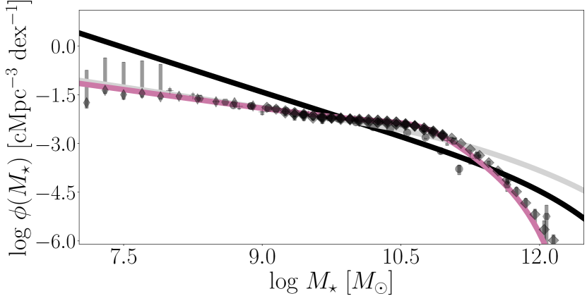
results in the number density function having distinct slopes on either end of the mass scale $M_{\mathrm{h}}\approx M_{\mathrm{c}}$, as long as $\gamma+\delta>1$. This is in agreement with observational evidence that the galaxy stellar mass function and UV luminosity function are more accurately described by a double Schechter function, in contrast to the single Schechter function that describes the halo mass function (Tomczak et al., 2014; Weigel et al., 2016; McLeod et al., 2021). Finally, note that for $\gamma=\delta=0$ (a model without feedback), the relation turns into $q\propto M_{\mathrm{h}}$ and $\diff{\log q}{\log M_{\mathrm{h}}}(M_{\mathrm{h}})=1$. The resulting number density is therefore identical in shape to the HMF, but shifted by $A/2$. If $\gamma\neq 0$ and $\delta=0$, we get a model without AGN feedback where the number density that is suppressed at the low mass end but traces the HMF at high masses. In Figure 1, we show model galaxy stellar mass functions for all three cases imposed on observations at $z=0$. It is evident that both feedback mechanisms are needed in order to reproduce the shape of the observed GSMF.

2.3 Supermassive Black Holes

Despite the challenge of estimating the masses and properties of SMBHs, particularly for those that are not actively accreting, tight correlations between the properties of supermassive black holes and their host galaxies have been robustly established at low redshift, suggesting a co-evolution between the two. This is primarily demonstrated by the stellar mass – velocity dispersion ($M-\sigma$) relation (Gebhardt et al., 2000; Ferrarese & Merritt, 2000; Davis et al., 2017), and to a lesser extent, the black hole mass-bulge mass (Kormendy & Ho, 2013) and black hole mass-stellar mass (Reines & Volonteri, 2015) relations. Given that stellar properties are closely linked to halo properties, we can connect the observed SMBH number density directly to the halo mass function in a similar fashion as for the galaxy properties. In this work, we will specifically focus on the black hole mass function (BHMF) and the bolometric luminosity function of active black holes, also known as the Quasar luminosity function (QLF).

2.3.1 Black Hole Mass Function

In accordance with the three regimes of galaxy formation we have discussed earlier, we model black hole growth to occur in three distinct phases: a slow growth phase in the stellar feedback regime, rapid growth in the turnover phase and slower growth again in the AGN feedback regime. This picture is supported by the empirically discovery that SMBHs growth appears to commence anti-hierarchically, with more massive SMBH forming first (Kelly & Shen, 2013). A simple parametrization for this idea is given by be

$$M_{\bullet}=B\cdot\begin{cases}\left(\frac{M_{\mathrm{h}}}{M_{\mathrm{c}}^{\bullet}}\right)^{\eta_{1}}&\text{for }M_{\mathrm{h}}\ll M_{\mathrm{c}}^{\bullet},\\ \left(\frac{M_{\mathrm{h}}}{M_{\mathrm{c}}^{\bullet}}\right)^{\eta_{2}}&\text{for }M_{\mathrm{h}}\approx M_{\mathrm{c}}^{\bullet},\\ \left(\frac{M_{\mathrm{h}}}{M_{\mathrm{c}}^{\bullet}}\right)^{\eta_{3}}&\text{for }M_{\mathrm{h}}\gg M_{\mathrm{c}}^{\bullet},\\ \end{cases}$$ (7)

where we expect $\eta_{2}>\eta_{1}>\eta_{3}$. However, as will be come clear in the following sections, the observational datasets we use are restricted to actively accreting black holes, suggesting the available data to only constraint the rapid growth phase. We will therefore restrict our model to a single power law,

$$M_{\bullet}=B\cdot\left(\frac{M_{\mathrm{h}}}{M_{\mathrm{c}}^{\bullet}}\right)^{\eta}.$$ (8)

The derivative of this equation is

$$\diff{\log M_{\bullet}}{\log M_{\mathrm{h}}}=\eta,$$ (9)

which is similar to the low mass behaviour of Equation 4 and similarly flattens the slope of the power law part of the number density function.

2.3.2 Quasar Luminosity Function

Actively accreting supermassive black holes are among the brightest objects in the Universe, resulting in the QLF being well-sampled up to $z\sim 3$ and partially constrained up to $z\sim 7$. This makes it the primary tool for understanding AGN evolution, with the bolometric luminosity of AGN in particular being tightly connected to the accretion rate of the black holes. Unlike the previous quantities, the number statistics of AGN luminosities differ qualitatively from the that of the halo masses. While the GSMF and UVLF are well-described by a Schechter function similar to the HMF, and arguments can be made that the BHMF has a similar functional form, the QLF is better described by a broken power law (e.g. Hasinger et al., 2005; Schneider et al., 2010; Ueda et al., 2014). It is challenging to reproduce this form using the formalism presented up to this point, as it is based on the HMF, which has an asymptotically exponential behavior. This difference can be linked to the much weaker correlation of the bolometric luminosity to the black hole mass (and thus halo mass, as described by our BHMF model), compared to the other quantities. In theory, two SMBHs of the same mass, hosted by halos of identical mass, can have bolometric luminosities that differ by tens of orders of magnitude, ranging from effectively inactive black holes that have no detectable emissions to luminosities that are close to the Eddington limit or beyond. In the literature, it is common to describe the relation between the black hole mass and bolometric luminosity using the Eddington luminosity relation

$$L_{\mathrm{bol}}=\lambda\cdot 10^{38.1}\cdot\frac{M_{\bullet}}{M_{\odot}}\quad\mathrm{erg\,s^{-1}},$$ (10)

where $\lambda$ is the Eddington ratio and $L_{\mathrm{bol}}(\lambda=1)$ is the Eddington luminosity.

The Eddington ratio for a given SMBH depends on physical quantities beside the black hole mass, and the exact relations are still poorly understood. In modelling approaches, it is therefore common to to assume the Eddington ratio to be a random variable following an Eddington ratio distribution function (ERDF), commonly denoted $\xi(\lambda)$, which may depend on black hole mass, halo mass, redshift and various other quantities, such as the central gas density and temperature. We can include this intrinsic spread in our model, by arguing that the observed bolometric luminosity function is the expectation value over all possible values of $\lambda$ weighted by the probability for a given $\lambda$ as given by the ERDF,

$$\phi(L_{\mathrm{bol}})=\int_{0}^{\infty}\phi_{\lambda}(L_{\mathrm{bol}},\lambda)\xi(\lambda)d\lambda.$$ (11)

Various shapes and functional dependencies of the ERDF have been proposed in the literature (see Shankar et al., 2013). Caplar et al. (2015), and subsequently Weigel et al. (2017), have shown that a $M_{\mathrm{h}}$-independent ERDF with a power law-like behaviour as $\lambda\rightarrow\infty$ is able to reproduce the bright end behaviour of the QLF. Caplar et al. (2015) have calculated the ERDF with an unbroken as well as a broken power law form and found that in this approach the faint end of the QLF is only weakly affected by the chosen ERDF, while the bright end is dominated the the $\lambda\rightarrow\infty$ behaviour of the ERDF and insensitive to the $\lambda\rightarrow 0$ end. Following this approach, we construct the QLF model using the following ingredients:

$$L_{\mathrm{bol}}=C\cdot\lambda\cdot\left(\frac{M_{\mathrm{h}}}{M_{\mathrm{c}}^{\mathrm{bol}}}\right)^{\theta},$$ (12)

$$\diff{\log L_{\mathrm{bol}}}{\log M_{\mathrm{h}}}=\theta$$ (13)

$$\xi(\lambda)\operatorname{d\!}\lambda=\frac{\frac{1}{1+\left(\frac{\lambda}{\lambda_{\mathrm{c}}}\right)^{\rho}}}{{\int_{-\infty}^{\infty}}\frac{1}{1+\left(\frac{\lambda}{\lambda_{\mathrm{c}}}\right)^{\rho}}\operatorname{d\!}\lambda}\operatorname{d\!}\lambda,$$ (14)

$$\phi(L_{\mathrm{bol}})=\int_{0}^{\infty}\phi_{\mathrm{\lambda}}(L_{\mathrm{bol}},\lambda)\xi(\lambda)d\lambda,$$ (15)

where Equation 12 is the relation between halo mass and bolometric AGN luminosity with ($C,\theta$) being free parameters, Equation 14 being the ERDF with ($\lambda_{c},\rho$) being free parameters. The model for the observed QLF is calculated using Equation 15, where $\phi_{\mathrm{\lambda}}$ is calculated using Equation 3 and Equation 13. The value under the integral in Equation 15 is the contribution to the bolometric luminosity function for a given value of $\lambda$, and if normalised to unity represents the conditional probability of a observing a given Eddington ratio for a fixed bolometric luminosity, i.e.

$$\xi(\lambda|L_{\mathrm{bol}})=\frac{\phi_{\lambda}(L_{\mathrm{bol}},\lambda)\xi(\lambda)}{\int\phi_{\lambda}(L_{\mathrm{bol}},\lambda)\xi(\lambda)}.\operatorname{d\!}\lambda,$$ (16)

It is worth noting that this function can vary for different bolometric luminosities even though the original ERDF was assumed mass-independent, due to the varying number densities of halos for different masses. An example of this is shown in Figure 2. The conditional distribution has a maximum approximately when $\phi_{\mathrm{bol,\lambda}}(L_{\mathrm{bol}},\lambda)\approx\xi(\lambda)$. In the limit $\lambda\rightarrow 0$ it is dominated by the exponential decay of the HMF and asymptotically has the same exponential behaviour, while in the limit $\lambda\rightarrow\infty$ the function decays as a power law (under the assumption that the HMF has a power law-like behaviour in the low mass limit), the asymptotic slope of $\xi(\lambda|L_{\mathrm{bol}})$ is given by $-\left(\rho-\frac{\alpha_{\mathrm{HMF}}}{\theta}\right)$. Note that we require $\rho>1$ in order for the ERDF to be normalisable and $\rho-\frac{\alpha_{\mathrm{HMF}}}{\theta}>1$ in order for the $\phi_{\mathrm{bol}}$ integral to converge. The cumulative distribution function for Equation 14 is given by $F(\lambda)=\lambda\cdot{}_{2}F_{1}\left(1,\frac{1}{\rho};1+\frac{1}{\rho},\left(\frac{\lambda}{\lambda_{\mathrm{c}}}\right)^{\rho}\right)$, where ${}_{2}F_{1}(\lambda)$ is the hypergeometric function. If the previous conditions are met, the resulting observed bolometric luminosity function will have the shape of a broken power law with an asymptotic faint end slope $\frac{\alpha_{\mathrm{HMF}}}{\theta}$ and an asymptotic bright end slope $-\rho$.

Figure 2: Luminosity-Dependence of the Conditional ERDF: While our ERDF model given by Equation 14 is independent of halo and black hole properties, the conditional ERDF defined by Equation 16 varies as a function of the bolometric luminosity: higher luminosities are associated with larger Eddington ratios due to the lower number density of high mass black holes. Shown are the conditional ERDFs for a set of luminosities at $z=0$ and $(C,\theta,\lambda_{\mathrm{c}},\rho)=(40,2,-2,2)$.

2.4 Relation Between Observable Properties

Since in our model all observable quantities are dependent solely to the halo mass (and redshift) through invertible relations, we can express any observable quantity $q_{1}$ as a function of any other quantity $q_{2}$ by $q_{1}(M_{\mathrm{h}})=q_{1}\left(M_{\mathrm{h}}(q_{2})\right)=q_{1}(q_{2})$. This allows us to study the relations between these quantities directly from their observed number densities. In particular we are able to relate galaxy and black hole properties using this method.

We choose to study the performance of our model (Section 4) using three relations:

• The galaxy stellar mass – UV luminosity relation: A proxy for the galaxy main sequence which has been robustly observed up to at least $z=6$ (Santini et al., 2017).

• The SMBH mass – stellar mass relation: One of the main clues that SMBHs and galaxies might co-evolve and well established at low redshift, albeit with a large scatter than the $M$ – $\sigma$ relation.

• The SMBH mass – AGN bolometric luminosity relation: One of the main avenues to study AGN and black hole accretion.

The asymptotic limits of the $M_{\bullet}$ – $M_{\star}$ and $L_{\mathrm{UV}}$ – $M_{\star}$ relations can be easily calculated since their parameterizations are all asymptotically power laws, resulting in the same behaviour for the interrelations between observable quantities. For example, combining Equation 4 and Equation 8 yields $M_{\bullet}\sim M_{\star}^{\nicefrac{{\eta}}{{(1+\gamma_{\star})}}}$ for $M_{\mathrm{h}}\ll M_{\mathrm{c}}$. The power law slopes for these two relations and different limiting cases of $M_{\mathrm{h}}$ can be found in Table 2.

The situation is a little more complicated for the $M_{\bullet}$ – $L_{\mathrm{bol}}$ relation, due to the adapted approach for modelling the QLF. Combing the relations for black hole mass and bolometric luminosity given by Equations 8 and 12 yields $L_{\mathrm{bol}}\sim\lambda\cdot M_{\bullet}^{\nicefrac{{\eta}}{{\theta}}}$, with behaviour of this relation depending on the distribution of $\lambda$: if the AGN sample selection is based on the host halo mass, the form of Equation 14 guarantees that the expectation value $\langle\lambda\rangle=\int\lambda\xi(\lambda)\operatorname{d\!}\lambda$ is $M_{\mathrm{h}}$-independent and $\langle L_{\mathrm{bol}}\rangle\sim M_{\bullet}^{\nicefrac{{\eta}}{{\theta}}}$ behaves as a power law. In practice, AGN samples are however primarily selected on luminosity, so that we have to use

$$\langle\lambda|L_{\mathrm{bol}}\rangle=\int\lambda\xi(\lambda|L_{\mathrm{bol}})\operatorname{d\!}\lambda=\frac{\int\lambda\phi_{\lambda}(L_{\mathrm{bol}},\lambda)\xi(\lambda)}{\int\phi_{\lambda}(L_{\mathrm{bol}},\lambda)\xi(\lambda)}\operatorname{d\!}\lambda,$$ (17)

which will differ for varying values of $L_{\mathrm{bol}}$, altering the functional form of the relation.

Table 2: Power law slopes for black hole mass $M_{\bullet}$ – stellar mass $M_{\star}$ relation and UV luminosity $L_{\mathrm{UV}}$ – stellar mass $M_{\star}$ relation for different halo mass limits.

Relation	$M_{\mathrm{h}}\rightarrow 0$	$M_{\mathrm{h}}\approx M_{\mathrm{c}}$	$M_{\mathrm{h}}\rightarrow\infty$
$M_{\bullet}$ – $M_{\star}$	$\nicefrac{{\eta}}{{(1+\gamma_{\star})}}$	$\eta$	$\nicefrac{{\eta}}{{(1-\delta_{\star})}}$
$L_{\mathrm{UV}}$ – $M_{\star}$	$\nicefrac{{(1+\gamma_{\mathrm{UV}})}}{{(1+\gamma_{\star})}}$	$1$	$\nicefrac{{(1-\delta_{\mathrm{UV}})}}{{(1-\delta_{\star})}}$

3 Observational Datasets And Model Calibration

Figure 3: Credible Regions of Modelled Galaxy Stellar Mass Functions: The model number densities as calculated from Equation 3 matched to observational data. The credible regions cover (in decreasing order of color saturation) 68%, 95% and 99.7% of the posterior distributions. The shaded area in the background marks the regime where the two feedback mechanisms contribute about equally to the stellar mass – halo mass relation given by Equation 4, the white area on the low mass side is dominated by stellar feedback, $(\left(\nicefrac{{M_{\mathrm{h}}}}{{M_{\mathrm{c}}^{\star}}}\right)^{\delta_{\star}+\gamma_{\star}}<0.1)$, while the area on the high mass side is AGN feedback-dominated, $\left(\nicefrac{{M_{\mathrm{h}}}}{{M_{\mathrm{c}}^{\star}}}\right)^{\delta_{\star}+\gamma_{\star}}>10$. The regime borders are calculated as the median value from a sample of GSMFs drawn from the posterior.

Figure 4: Credible Regions of Modelled Galaxy UV Luminosity Functions: Similar to Figure 3. Here, the white region on the bright side is AGN feedback-dominated regime, while the area on the faint end is stellar feedback dominated.

Figure 5: Credible Regions of Modelled Black Hole Mass Functions: Note that the available data does not constitute the full BHMF, but the mass function of Type 1 AGN (Section 3.1.3).

Figure 6: Credible Regions of Modelled Quasar Luminosity Functions: The ERDF parameter $(\lambda_{\mathrm{c}},\rho)$ are free at $z=0$, but fixed to the $z=0$ MAP estimates $(\lambda_{\mathrm{c}},\rho)\approx(-2.2,1.4)$ for $z>0$.

The strength our simple empirical model is not found in precise quantitative predictions, but rather a qualitative understanding of the evolution and importance of the physical mechanisms involved. For this reason, we turn to a probabilistic approach for calibrating our model: rather than focusing on expectation values or best-fit parameter, we study the evolution of the probability distributions for the parameter as a whole. This approach leverages the computational simplicity of the model and is especially useful for sparsely sampled data (e.g. at high redshift) and when making predictions beyond current observational limits. In this section, we describe the datasets used to calibrate the model, the statistical framework and assumption made for the statistical inference in order to match the observed number density functions.

3.1 The Datasets

We have collected observational dataset from a variety of sources and homogenized (e.g. for the assumed IMF) in order for them to be comparable. Nonetheless, there will be differences in the way the data was processed by the original authors. We try to take this into account by adding an additional uncertainty whenever dataset from multiple authors are used. (see Section 3.2 for details).

3.1.1 GSMF Data

We collect data on the GSMF from a variety of sources (Baldry et al., 2012; Moustakas et al., 2013; Ilbert et al., 2013; Duncan et al., 2014; Tomczak et al., 2014; Song et al., 2016; Davidzon et al., 2017; Bhatawdekar et al., 2018; Stefanon et al., 2021) spanning $z=0$ – $10$, correcting the data for assumed IMF (we employ a Chabrier (2003) IMF with a mass range of $0.1$–$100M_{\star}$) when necessary and re-binning into integer redshift bins (e.g. mapping $0.5\leq z\leq 1.5$ to $z\sim 1$). The stellar masses have primarily been constructed by SED fitting to available photometry, and have been corrected for dust extinction. The GSMF is best described by a double Schechter function for $z<3$ (Davidzon et al., 2017), while at higher redshift a single Schechter function suffices. The low mass slope of the GSMF has been robustly found to decrease towards lower redshift, while the overall number density increases.

3.1.2 Galaxy UVLF Data

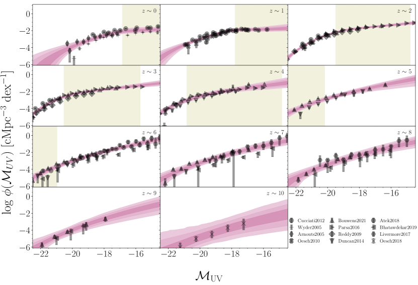
The galaxy UV luminosity (rest frame wavelength centred around $\lambda\approx 1500$-$1600$ Å) data also spans a redshift range from $z=0$ – $10$, collected from multiple sources (Wyder et al., 2005; Parsa et al., 2016; Cucciati et al., 2012; Duncan et al., 2014; Atek et al., 2018; Arnouts et al., 2005; Livermore et al., 2017; Bhatawdekar et al., 2018; Bouwens et al., 2021). The provided data is corrected for dust extinction, and when necessary is adjusted for different IMFs. The UVLF is best constrained for $z\geq 2$ for which the rest frame UV is redshifted to the optical and IR bands. The UVLF peaks across most luminosities around $z=2$ – $3$, which is known to be the peak of star formation (cosmic noon) and drops towards higher and lower redshift. Similar to the GSMF, the UVLF slope increases robustly between $z=2$ and $z=10$, with some debate on the evolution on the very faint end (Bowler et al., 2015, 2017; Harikane et al., 2022). The evolution for $z<2$ is more strongly contested but seemingly consistent with a constant slope (Cucciati et al., 2012).

3.1.3 Data On The Active BHMF Of Type 1 AGN

While we have managed to construct a model relating the mass of SMBHs to that of their halos, the remaining challenge are the observational constraints of the BHMF. Current constrains on the SMBH masses from direct kinematic modelling are limited to a small sample of local galaxies (Kormendy & Ho, 2013) from which no reliable number statistics can be discerned. Larger and more distant samples can be inferred using indirect methods in AGN, predominantly by estimating velocity dispersion (and consequently virial mass) of the accretion disk from the broad line emission width for Type 1 (unobscured) AGN (Vestergaard & Peterson, 2006), although broad line - narrow line correlations have been used to extend the estimation to Type 2 (obscured) AGN as well (Baron & Ménard, 2019). These types of studies can be used to constrain the BHMF up to $z=5$ (Kelly & Shen, 2013), but with the caveat that these are limited to the sub population of active black holes rather than the total black hole population. We employ the active black hole mass function of Type 1 AGN as collected by Zhang et al. (2021) based on the work of Schulze & Wisotzki (2010), Kelly & Shen (2013) and Schulze et al. (2015). These active BHMFs follow the known evolution of the AGN population: number densities peak between $z=2$ and $3$, which corresponds to the era of peak star formation and black hole growth (and thus increased black hole activity), and number densities at high masses dropping faster towards low redshift compared to lower mass black holes (cosmic downsizing). It needs to be stressed that the relation between the number densities of Type 1 AGN and the total SMBH population is not trivial and that we have not included a mechanism in our model that accounts for this selection of the sub-population. Interpreting the results of the redshift evolution of the BHMF and relating the black hole masses to other quantities in the model therefore needs to be done in light of this limitation (see Section 4).

3.1.4 QLF Data

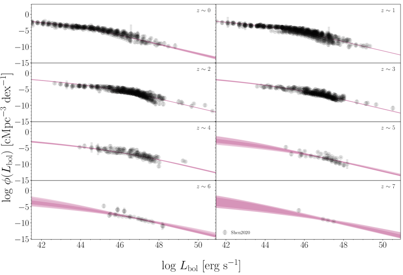
We employ the quasar bolometric luminosity functions constructed by Shen et al. (2020) covering $z=0$-$7$ . These QLFs are based on observations in the IR, optical, UV and X-ray bands from which the bolometric luminosities have been constructed using a template quasar SED constructed by the authors, where the bolometric luminosity is defined to cover from the range 30$\mu$m (far IR) up to 500keV (ultra-hard X-ray). The QLFs show a considerable redshift evolution in normalisation as well as slope, with similar signs of cosmic downsizing (Cowie et al., 1996; Hasinger et al., 2005). For example, the number density of AGN with $\log L_{\mathrm{bol}}\approx 46$ erg s^-1 appear to peak at $z\approx 2.4$ (Shen et al., 2020).

Figure 7: The Galaxy UV Luminosity – Stellar Mass Relation at $\mathbf{z=4-7}$ : The purple line shows the model median, with the shaded area being as the 95% credible region. The reference data is obtained from Song et al. (2016, grey points), while the grey lines are their reported best-fit $\log(M_{\star})$ – $\mathcal{M}_{\mathrm{UV}}$ relations.

3.2 Optimization Prescription: Likelihood Function And Priors

We construct the parameter probability distributions using a least squares approach and sample the posterior distributions using the MCMC algorithm emcee (Foreman-Mackey et al., 2013). We assume a Gaussian likelihood function

$$\ln\mathcal{L}(z;p)=-\frac{1}{2}{\sum_{i}}\left[\frac{\mathrm{R}_{i}(z;p)^{2}}{s_{i}(z;p)^{2}}+\ln\left(2\pi s_{i}(z;p)^{2}\right)\right],$$ (18)

where we calculate the residuals $R_{i}(z;p)=\log\phi_{\mathrm{obs}}\left(q_{i},z\right)-\log\phi_{\mathrm{model}}\left(q_{i}(M_{\mathrm{h}}),z;p\right)$ in log space. For the BHMF and QLF, which were collected from a single source each, we use the relative uncertainties to weight the residuals, $s_{i}(z;p)=r_{i}(q_{i})$ (we use the relative uncertainties since we work in log space), while we consider two contributions to the variance for the GSMF and UVLF, $s_{i}(z;p)=r_{i}(q_{i})+\sigma\left(R_{i}(z;p)\right)$: in addition to the reported uncertainties, combining the data from multiple groups introduces an additional systematic uncertainty since every group performs the data reduction in their own ways using varying assumptions and methods (such as dust correction prescription, SED templates, etc.). It is prohibitively difficult to account for these discrepancies in detail, so for simplicity we assume a Gaussian distribution for these effects and use the variance of the residuals $\sigma^{2}\left(R_{i}(z;p)\right)$ as an estimate for the spread of this distribution.

A simple, redshift-independent prior would be a set of independent uniform distributions for every parameter within some sensible bounds $a_{i}$, $P_{z}(p_{i})=\mathcal{U}_{[a_{i},b_{i}]}$, with $a_{i}$ and $b_{i}$ being the lower and upper bounds for the parameter $p_{i}$, respectively, so that the total prior probability is given by $P(p)=\prod_{i}P(p_{i})$. This approach assumes that initially, all possible parameter combinations are equally likely and only the data given in a redshift bin alters the probability for the parameter. We however choose a successive prior approach, meaning we use the posterior distribution at a redshift $z$ as prior for the distribution at redshift $z+1$, so that the posterior is given by $P_{z}(p)=\frac{\mathcal{L}(z;p)P_{z-1}(p)}{\int\mathcal{L}(z;p)P_{z-1}(p)\operatorname{d\!}p}$, where $\mathcal{L}$ is the likelihood function defined in Equation 18 and we assume a uniform prior at $z=0$. In essence, this approach adds the additional assumption that, if an evolution in the parameter occurs, this evolution will be gradual and smooth across redshift so that distributions should not widely differ between different redshift bins. By starting with this baseline assumption, we can make use of the stronger constraints at low redshift (where more data is available) and work ourselves up to the less constrained redshift regime, at the cost of the distributions not being independent between redshift bins.

3.3 Recreating The Population Statistics

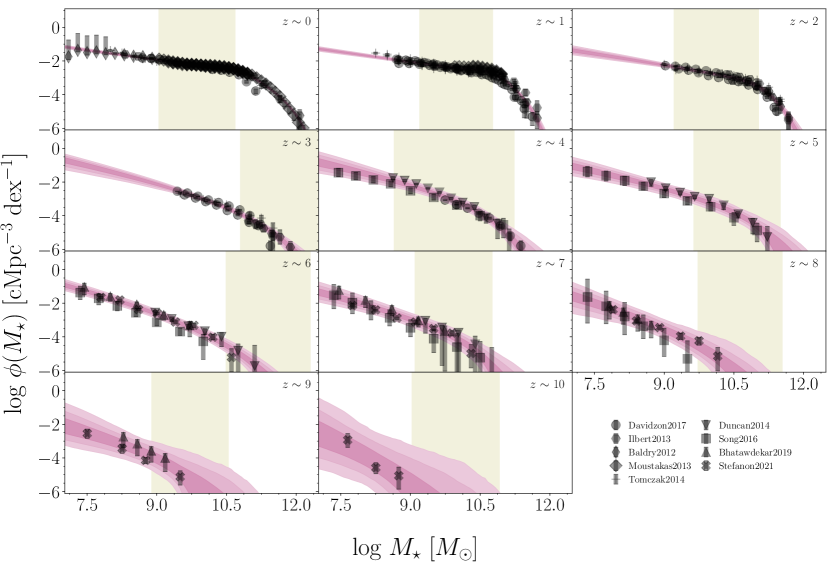
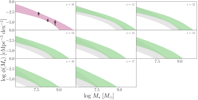
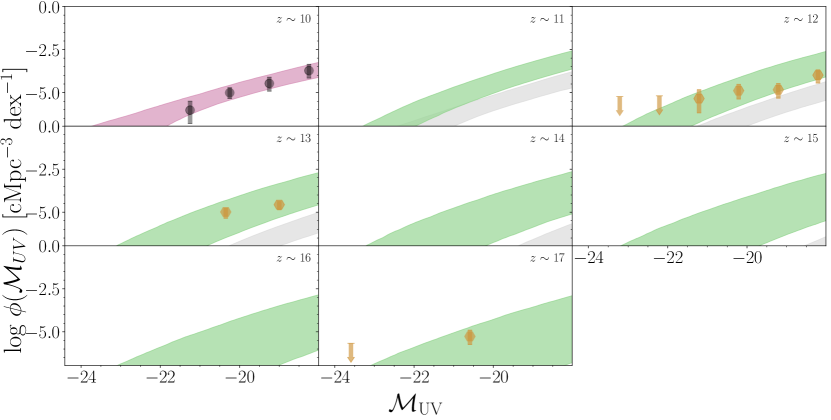
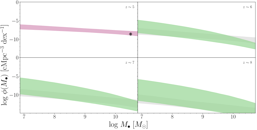
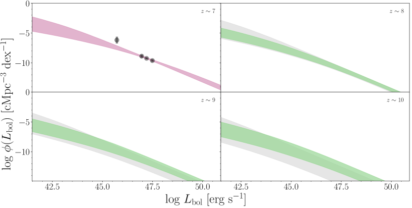
We constrain the free parameters of the model by matching the observed number density functions (Section 3.1) to our model (Section 2) using the previously described probabilistic approach (Section 3.2); from this we obtain probability distributions for the parameter which can be used to create sample number density functions. A summary of the parameter distributions can be found in Appendix C. The result of this procedure is shown in Figures 3, 4, 5 and 6 where we mark the 68%, 95% and 99.7% credible regions for the average number densities at every redshift. In order for the parameter distributions to be well-behaved, especially at high redshift where data is sparse, we have to make a number of additional assumptions:

• For the GSMF and UVLF, we treat the the critical mass $M_{\mathrm{c}}$ and AGN feedback parameter $\delta$ as free parameters up to redshift $z=2$ and $4$, respectively. At higher redshift, the two parameter are marginalised over when needed, since the AGN-dominated regime is not sampled (see Figures 3 and 4) and the parameter weakly constrained.

• For the GSMF, we enforce an upper limit on the normalisation parameter A so that ${M_{\star}}/{M_{\mathrm{h}}}$ peaks at the cosmic baryon fraction $\approx 0.2$.

• For the BHMF and QLF, we fix the critical mass $M_{\mathrm{c}}$ to the most likely parameter estimates, given by the maximum a posteriori (MAP) estimator, of the GSMF to reduce complexity of the model.

• For the QLF, we fix the parameter of the ERDF ($\lambda_{\mathrm{c}}$, $\rho$) for $z>0$ to the MAP estimates at $z=0$, i.e. assume an unevolving ERDF.

The limited availability of data on the high mass end of the GSMF and bright end of the UVLF due to low number density make it impossible to study the parameter evolution of $M_{\mathrm{c}}$ and $\delta$ in detail, however the number densities can still be closely matched when treated as nuisance parameter and some information about their evolution can be inferred (see Section 5). There is no strong reason to assume the ERDF is unevolving, however the observations are still reasonably well reproduced at higher redshift justifying this assumption. Note that the distributions for the bright end of the QLF are extremely localized for $z=1$-$3$; this is exemplifies that the bright end is completely determined by the shape of the ERDF (while the faint end is strongly constrained by the amounts of available observations).

4 Assessing The Relation Between Observables

In the previous section, we demonstrated that our model is able to produce number densities that closely match available observations. However, using observed number densities to constrain the model parameters is not a sufficient indicator of the model’s performance. To truly assess the model’s validity, we must also compare the model output to data that was not used in the calibration process. Since a key feature of the model is the ability to relate different observable quantities (see Section 2.4), it in insightful to compare these interrelations to available datasets.

Figure 8: The SMBH Mass – Galaxy Stellar Mass Relation at $\mathbf{z=0}$: The reference observations are obtained from Baron & Ménard (2019) for a sample of Type 1 and Type 2 AGN at $z<0.3$. The purple line shows the model median and the 95% credible region. The grey and black lines show the relation using MAP estimates for the parameter of the GSMF and BHMF models when the observed SMBH mass number densities are scaled up by a factor of 10, 30 and 100, respectively.

4.1 Galaxy Stellar Mass – UV Luminosity Relation

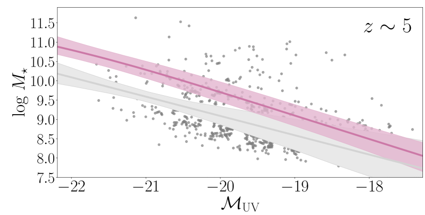
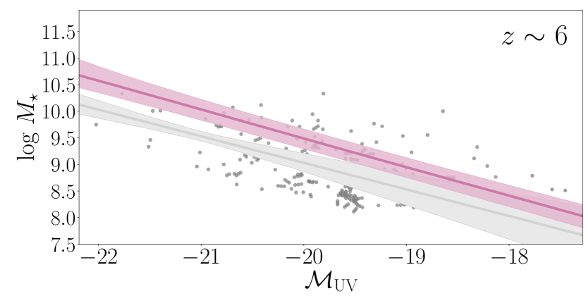
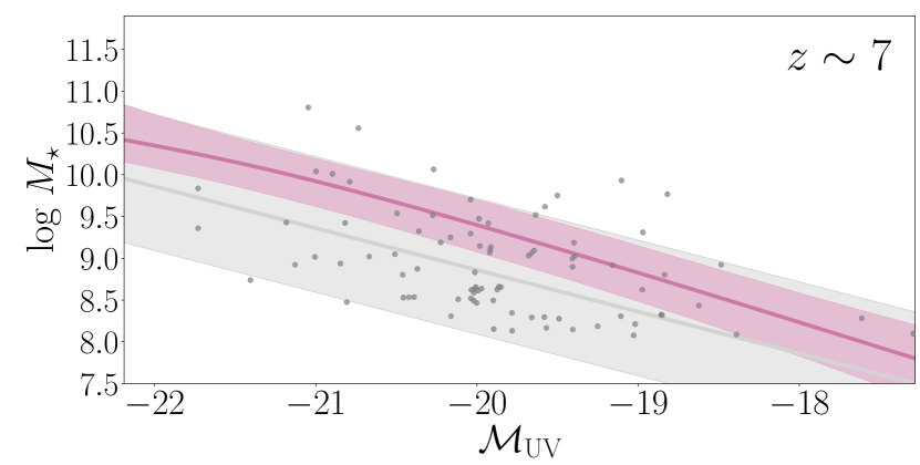
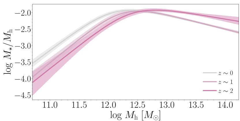
The galaxy main sequence is a well-studied near-linear relation between the stellar mass and star formation rate (SFR) of star-forming galaxies (Brinchmann et al., 2004; Whitaker et al., 2014; Sherman et al., 2021), and since the intrinsic UV luminosity of a galaxy is a tracer of the instantaneous star formation rate, the stellar mass – UV luminosity relation can be used as a proxy to study the evolution of the galaxy main sequence. We gather data on this relation from Song et al. (2016) covering $z=4$-$7$; this redshift range is ideal to study our model output since the GSMF and UVLF are well-sampled over this range. Figure 7 shows the expected relation obtained from the model compared to the observational data. The model falls within the range of observations but consistently overpredicts stellar masses for a given UV luminosity when compared to the $\log(M_{\star})$ – $\mathcal{M}_{\mathrm{UV}}$ relation as inferred by Song et al. (2016).

A hint for a potential resolution of this mismatch can be found in the data itself: for a fixed luminosity bin, the stellar mass distribution is strongly skewed, being more spread out towards high masses. This can be reasoned by the data most likely covering two distinct galaxy populations: those galaxies that are actively star-forming and follow the main sequence, leading to a tight relation in the $\log(M_{\star})$ – $\mathcal{M}_{\mathrm{UV}}$ plane, and a population of dusty star-forming or quiescent galaxies as might be hinted at from recent JWST observations (Naidu et al., 2022). Note that the asymmetry increases towards lower redshift as the (observed) quiescent fraction increases. The modelled relation falls roughly midway between the minimum and maximum observed stellar mass per luminosity bin, suggesting that the source of the mismatch is our model assumption of a one-to-one relation between stellar mass/UV luminosity and halo mass given by Equation 4. This is a simplifying assumption, as one in reality would expected a distribution of stellar masses and UV luminosities for a given halo mass. Indeed, recent ALMA observations are beginning to show galaxies that lie significantly above the ”main sequence” (Algera et al., 2023). If this distribution were symmetric and reasonably localized, it would not strongly affect the expected stellar mass/UV luminosity – halo mass relation and primarily create a scatter around the relation. However, the distributions being skewed as hinted at here (so that the expectation value is identical but a large part of the distribution is concentrated around values lower or higher than the expectation value) may lead to an overestimation of the modelled mean values due to lower mass halos contributing more strongly owing to their intrinsic higher number densities. In principle, this effect can be taken into account in the model by including this asymmetric distribution using the machinery described in Appendix B, but in practice the distribution of stellar mass/UV luminosity for a given halo mass is hard to constrain observationally; an proof-of-concept example is shown in Figure 18. At this stage, the model reproduces the stellar mass – UV luminosity relation reasonably well given the simplicity of the model and scatter in the observed relation, but it is good to keep this systematic bias in mind if the model is used in practice.

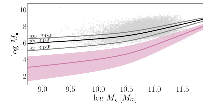
4.2 SMBH Mass – Galaxy Stellar Mass Relation

Besides being able to connect different stellar properties of the galaxies, we are also able link stellar and AGN properties using our model. The relation between galaxy stellar mass and mass of the central SMBH is relatively well constrained in the local universe and suits itself to test our model. For this we use the dataset gathered by Baron & Ménard (2019) for Type 1 and Type 2 AGN at $z<0.3$. Figure 8 shows the SMBH mass as a function of stellar mass as obtained from our model at $z=0$. It is quite clear, that the model systematically underpredicts the black hole mass for a given stellar mass, and that this discrepancy becomes more pronounced at low stellar masses. This mismatch is not surprising, since the black hole mass functions we used to constrain our model are for Type 1 AGN only, which constitutes only a sub-population of all AGN and more generally a sub-population of all SMBH (see Section 3.1.3). Since our model connects observable quantities through their number densities, and we effectively underestimate the number density of SMBH by only considering this sub-population, a systematic bias towards lower black hole masses is produced. To get a consistent stellar mass - black hole mass relation using our model, we would need a black hole mass function for all SMBH and not only Type 1 AGN, which is observationally hard to constrain for non-active black holes, especially at high redshift. However, studies suggest that selection biases in the observation of active and non-active populations lead to a discrepancy in their respective $M_{\bullet}$ – $M_{\star}$ relations (Shankar et al., 2016, 2019).

We can easily study the effect an increased number density of BHs by simply scaling the BHMF by some constant value. A rough estimate for the appropriate magnitude can be obtained as follows: the BHMF we use is constructed exclusively for Type 1 AGN; Hatziminaoglou et al. (2009) suggests a Type 2-to-Type 1 ratio of  2-2.5 for their low-luminosity, low-redshift AGN sample. To a first approximation, we can therefore scale the observed active BHMF at $z=0$ by a factor of 3-3.5 to obtain an estimate for the mass function of all active SMBH.

Further, we need to estimate the ratio of active to non-active SMBHs. For this, we can use the ERDF obtained by the modelling the QLF (Section 2.3.2), and argue that SMBH below a cutoff Eddington ratio can be considered inactive. For this cutoff, we choose an Eddington ratio of $\lambda_{\mathrm{cutoff}}=0.01$, since this is the regime where AGN switch between Jet mode and radiative mode (Heckman & Best, 2014) and the because the sample collected by Baron & Ménard (2019) primarily contains supermassive black holes with $\lambda>0.01$. For the MAP parameter estimate of the ERDF at $z=0$, the probability of a randomly selected black hole have an Eddington ratio below 0.01 is  0.90 and since we assume our ERDF to be mass-independent this means we expect 1 in 10 black holes to be active. Therefore, to estimate the number densities of the full SMBH population, we scale the BHMF for all active SMBH by a factor of 10 (or consequently the observed BHMF for Type 1 AGN by a factor of 30-35). The calculated stellar mass - black hole mass function using this rescaled BHMF is shown in Figure 8 and constitutes a much closer match to the data.

Of course, the actual relation between the mass function for active Type 1 AGN and for all SMBH is a lot more complicated than this simple scaling. Gilli et al. (2007); Hatziminaoglou et al. (2009) and U (2022) suggest that the Type 2-to-Type 1 ratio evolves with black hole luminosity (with is in our model directly linked to black hole mass), and the ratio between active and non-active black holes (commonly described through the occupation fraction and duty cycle) is expected to evolve with black hole mass and redshift (Shankar et al., 2013; Volonteri et al., 2017; Heckman & Best, 2014) which is related to the cosmic downsizing discussed earlier. In particular, the fact that our way of estimating the active to non-active ratio using the ERDF, which is constructed using the quasar luminosity function (i.e. only active BHs) and is only weakly constrained on the low-Eddington ratio end (see Section 2.3.2), leads to such a good match to the available data may be in part a coincidence, but seems to suggest the correct order of magnitude increase needed to reconcile the model with the available data.

Figure 9: Distribution of Black Hole Masses for $\log L_{\mathrm{bol}}=45.2$ [erg s^-1] at $\mathbf{z=0}$: The purple line shows the model median distribution with the 95% credible region, while the histogram shows the observational data on Type 1 AGN gathered from (Baron & Ménard, 2019). The grey vertical lines show where the Eddington ratio reaches 0.01 and 1, which marks the boundaries where we expect additional effects to play a role that are not included in the model. The grey dotted line is the expected distribution calculated from the MAP parameter estimates, when invoking a hard cutoff outside of these boundaries. Doing so decreases the mismatch between the distribution means from 0.5 dex to 0.3 dex compared to the observational sample.

4.3 SMBH Mass – AGN Bolometric Luminosity Relation

Finally, we can connect the properties of active SMBH. As described in Section 2.4, the relation between black hole mass and AGN luminosity is a power law with a slope given by $\eta/\theta$, and since both parameters are assumed to be positive, the model predicts that average AGN luminosity increases with black hole mass. As argued before however, the number statistics of black hole masses plays a crucial role in observed black hole quantities. To include this effect, we can estimate the black hole mass distribution from the conditional ERDF (see Section 2.3.2) and calculating the mean black hole mass for every luminosity this way. This approach does not only take the intrinsic AGN luminosities into account, but also the number statistics of black hole masses. An added advantage to this approach is that is only requires information from the bolometric luminosity function, and therefore circumvents the uncertainties related with scaling the BHMF. At low luminosities, the number densities play no significant role and the produced relation is similar to the direct calculation (and is within model uncertainties and the proposed scaling of the BHMF). For luminosities $>10^{45}$ erg s^-1 (at $z=0$), the exponential drop in the BHMF becomes dominant and the expected black hole mass stops to grow with luminosity. Simply put, at $z=0$ active black holes with $M_{\bullet}>10^{8.5}M_{\odot}$ are expected to be so rare that high luminosities are much more likely caused by large Eddington ratios rather than very massive black holes. The difference between the two predictions is in essence a selection effect: if AGN are selected based on their luminosity (as is done in observational surveys), the flattening relation is to be expected. If the AGN were selected based on their mass (so that the number statistics of the BHMF play no role), we’d expect the simple power law relation.

In Figure 9, we show the the empirical black hole mass distribution from a luminosity-selected sample of ~2000 Type 1 AGN from Baron & Ménard (2019), with mean bolometric luminosity of $10^{45.2}$ erg s^-1 and a scatter of ~0.2 dex, and the modelled distribution obtained from the conditional ERDF. The two distributions are in overall good agreement, however the expected and observed mean black hole mass differ by ~ 0.5 dex and the model underpredicts the probability for high Eddington ratios (and vise versa) compared to data, as well as predicting wider tails to the distribution. At the bright end, the simple Eddington model of isotropic accretion breaks down for $\lambda\geq 1$. It is therefore expected that our model, which is built on the linear $L_{\mathrm{bol}}$-$M_{\bullet}$ relation derived from Eddington theory, would not match observations in this regime. Previous studies have shown that the fraction of AGN drops sharply for accretion rates with $\lambda\geq 1$ (Heckman et al., 2004). At the high mass end (low Eddington ratios, $\lambda\sim 0.01$), AGN tend to be more likely supported by advection-dominated accretion flows, with geometrically thick and optically thin accretion disks, which affects the black hole mass - luminosity relation as well as the ability to estimate black hole masses using broad line emissions (Narayan, 2005); similarly effects which we did not explicitly include in the model. The radiative mode – Jet mode transition does not occur at instantaneously at any specific Eddington ratio, but becomes more likely as the Eddington ratio decreases (Best & Heckman, 2012; Russell et al., 2013), which matches the discrepancy in our model for $\lambda\sim 0.01$. If we, for simplicity, invoke hard cutoffs for $\lambda<0.01$ and $\lambda>1$ (and normalise the distribution accordingly), the mismatch between expected and observed mean black hole mass decreases to ~0.3 dex, as can be seen from the dotted grey line in Figure 9.

5 Evolution Of The Population Statistics Over Cosmic Time

(a) Stellar mass function parameter sample. The critical mass parameter $M_{\mathrm{c}}^{\star}$ and AGN feedback parameter $\delta$ are weakly constrained at $z>2$ and treated as nuisance parameter at higher redshift.

(b) UV luminosity function parameter sample. The normalisation $A_{\mathrm{UV}}$ is given in erg s^-1 Hz^-1 $M_{\odot}^{-1}$.
.

(c) Type 1 active black hole mass function parameter sample.
.

(d) Quasar luminosity function parameter sample. The normalisation $C$ is given in erg s^-1 $M_{\odot}^{-1}$.

Figure 10: Parameter sample across redshift: A random sample of the model parameter drawn from the posterior distributions at every redshift. Increased color saturation indicates a larger value for the probability density.

With the validity of the model established and and potential caveats and pitfalls demonstrated, we can turn to redshift evolution of the model quantities. By matching the model to observations at every integer redshift bin individually, we obtain a non-parametric estimate of the observable quantity – halo mass relations throughout the observed redshift ranges. This section is split into two parts, first we interpret the evolution of the modelled number density function and compare it to more comprehensive modelling approaches, while the second part is focused on extrapolating the observed trends to as of yet unobserved redshift.

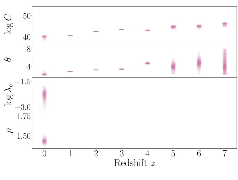
5.1 Comparison With Observations And Other Models

Figure 10 shows $10^{4}$ samples of the parameter posterior distribution drawn at every redshift bin and for every quantity, with the level of color saturation representing the posterior probability. The parameter distributions for the GSMF and UVLF (Figures 10(a) and 10(b)) are marginalised over the critical mass $M_{\mathrm{c}}$ and the AGN feedback parameter $\delta$ after $z=2$ and $z=4$, respectively.

5.1.1 Galaxy Evolution

(a) stellar mass – halo mass ratio at low redshift.

(b) stellar mass – halo mass ratio at high redshift. The shown ranges coincides with the observed GSMFs. The high mass slope is outside of the observed range.

Figure 11: stellar mass – halo mass ratio across redshift: The SHMR is calculated to the parameter samples shown in Figure 10. The purple line shows the model median while the shaded areas represent the 95% credible regions.

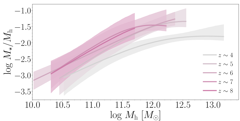
For the galaxy stellar mass function, we find the critical mass $M_{\mathrm{c}}^{*}$ increases with redshift up to the last constrained redshift bin $z=2$, as well as an increase in the overall normalisation parameter $A$ up to values close to cosmic baryon fraction at $z=6$. The feedback parameters $\gamma$ and $\delta$ vary somewhat over their respective redshift ranges but are consistent with little to no evolution. A clear way to analyse these trends is looking at the stellar mass – halo mass ratio (SHMR), shown in Figure 11. At $z<3$, the evolution of the SHMR is consistent with an unevolving slope and normalisation, with a robust change only in the critical mass (location of the turnover point in the SHMR). At $z>3$, we only plot the SHMR over the ranges we have observational data for the GSMF, which exemplifies that the AGN feedback-dominated high mass slope is unconstrained at high redshift. The stellar feedback-dominated low mass slope is is consistent with being unchanging within the credible regions of the model, while the critical mass seemingly decreases with increasing redshift. The normalisation is higher than at low redshift, but too uncertain to infer an evolution.

When compared to the SHMR obtained by a more comprehensive empirical model such as UniverseMachine (Behroozi et al., 2019), we find that the evolution of the critical mass and low mass slope are consistent with their results. On the other hand, in UniverseMachine the high mass slope of the SHMR consistently increases with redshift, while they find a stronger evolution in the normalisation which consistently decreases with redshift. UniverseMachine has a larger focus on environmental effects and constructs the galaxy properties by populating dark matter halo in a probabilistic fashion, which leads to a more diverse galaxy population compared to our simple model, which likely contributes to this discrepancy. In particular, Behroozi et al. (2019) find a redshift- and halo mass-dependent scatter in the stellar mass – halo mass relation, with an average of $\approx 0.25$ dex.

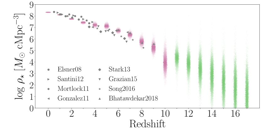
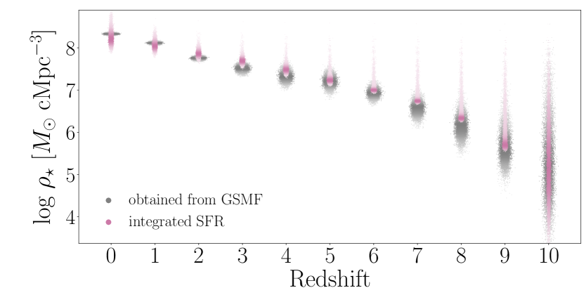
In Figure 19, we show the effects of scatter on our estimate of the GSMF, when calculated as described in Appendix B: The high mass slope highly sensitive to the amount of scatter, as well as the normalisation, while the low mass slope is unaffected, which are exactly the discrepancies found with UniverseMachine. This also explains why we find a consistently higher normalisation (which even approaches the cosmic baryon fraction at high redshift) in the stellar mass – halo mass relation. Nonetheless, in our model framework, we are able to reasonably reproduce the GSMF with an stellar mass – halo mass relation that only evolves in the critical mass and normalisation while feedback slopes are fixed. Further, we find the total stellar mass density, defined as

$$\rho_{M_{\star}}=\int_{\log M_{\star}^{\mathrm{min}}}^{\log M_{\star}^{\mathrm{max}}}M_{\star}\diff{n}{\log M_{\star}}\operatorname{d\!}\log M_{\star},$$ (19)

where we employ $M_{\star}^{\mathrm{min}}=10^{8}M_{\odot}$ and $M_{\star}^{\mathrm{max}}=10^{13}M_{\odot}$ for comparability with earlier studies, to decrease with redshift in a log-linear fashion (Figure 12(a)) that is consistent in slope and normalisation with observations (Bhatawdekar et al., 2018).

We find a a slightly different picture for the UV luminosity function (Figure 10(b)), where the posterior suggest an unchanging critical mass but a consistent increase in normalisation with redshift. The AGN feedback parameter is also consistent with being unchanging, while the stellar feedback parameter has larger values at $z=0$ and $z=1$ before decreasing to a more consistent value at larger redshift. It is likely that this behaviour at low redshift is caused by the comparably large spread in different estimates of the UVLF rather than physical effects, due to the lag of large UV surveys at low redshift, which manifests in the large uncertainties of the parameter estimates at low redshift. The estimates are much more robust for $z\geq 2$, when the emitted UV is shifted to the rest-frame optical bands. We show the integrated star formation rate for $z\geq 4$ in Figure 12(b). They are consistent with observational estimates for high redshift surveys (Oesch et al., 2018; Bhatawdekar et al., 2018) and shows a similar trend to UniverseMachine, although their estimated SFR density drops more slowly with redshift. For consistency, we compare the stellar mass density calculated from the GSMF to the one obtained by integrating the star formation rate density over cosmic time. To include all relevant contributions, we integrate the model GSMF and UVLF over the same range defined by through the halo mass, i.e. we integrate from compare $q^{\mathrm{min}}={q(M_{\mathrm{h}}^{\mathrm{min}})}$ to $q^{\mathrm{max}}={q(M_{\mathrm{h}}^{\mathrm{max}})}$ where we impose $M_{\mathrm{h}}^{\mathrm{min}}=10^{3}M_{\odot}$ and $M_{\mathrm{h}}^{\mathrm{max}}=10^{21}M_{\odot}$. The stellar mass density can be obtained from the star formation rate density using

$$\rho_{\star}^{\mathrm{UV}}(z) =\left(1-R\right)\int_{0}^{t(z)}\psi\operatorname{d\!}t^{\prime}$$

$$=\left(1-R\right)\int_{t(z=10)}^{t(z)}\psi\operatorname{d\!}t^{\prime}+\rho_{\star}(z=10),$$ (20)

where $R=0.41$ is the return fraction for a Chabrier (2003) IMF and $\rho_{\star}(z=10)$ is the stellar mass density obtained from integrating the GSMF at $z=10$. Figure 13 shows that both methods produce similar result for the stellar mass density. It is worth noting that this consistent result is not necessarily expected. Madau & Dickinson (2014), for example, show that the integrated star formation rate slightly overestimates the stellar mass density compared with direct measurements, particularly at $z<2$. Due to the relatively poor constraints on the UV luminosity function in this regime, we are however unable to find a statistically significant difference in our model.

(a) Stellar mass density.

(b) Star formation rate density.

(c) Type 1 active black hole mass density.

(d) AGN bolometric luminosity density.

Figure 12: Redshift evolution of the integrated densities: Integrated number density function calculated for a sample of model parameter drawn from the posterior. Increased color saturation indicates a larger value for the probability density. Distributions in purple have been constrained by data, while green distributions are linearly extrapolated. For Figure 12(a) and Figure 12(b), observations collected by Bhatawdekar et al. (2018) are shown in grey.

5.1.2 AGN Evolution

Figure 13: Evolution of the stellar mass density: Shown is are samples of the stellar mass density predicted by the model, calculated by integrating the GSMF at every redshift (grey) and by integrating the model star formation rate density over cosmic time (purple).

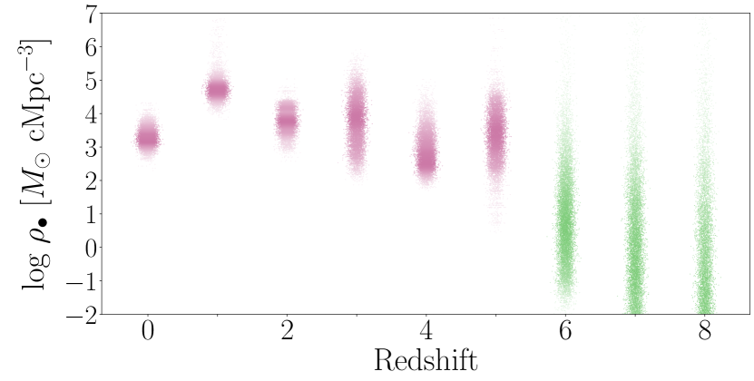
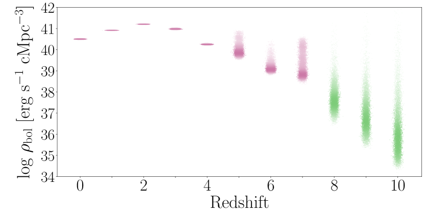
The parameter distribution for the mass function of the active Type 1 AGN (Figure 10(c)) show a consistent increase of the normalisation and slope as redshift increases, meaning the model suggests that at higher redshift SMBHs are more massive for a given halo mass and increase in mass faster with halo mass. This is consistent with cosmic downsizing as discussed earlier, and found in previous studies on the active BHMF (Kelly & Shen, 2013; Schulze et al., 2015). The comprehensive halo – galaxy – SMBH evolution model Trinity (Zhang et al., 2021) find similar results, in the sense that more massive black holes becomes less active earlier in cosmic time compared to smaller black holes. The evolution of the parameter distribution for the QLF (Figure 10(d)) is consistent with this finding, where the normalisation and slope similarly increase with redshift, meaning for a given halo mass the model predicts AGN to become more luminous with increasing redshift, under the assumption of a fixed Eddington ratio distribution function. Put together, this means the model predict that at higher redshift massive and luminous AGN will be hosted in lower mass compared to AGN at low redshift, suggesting that massive black holes grow early. This holds at least under the assumption of an unevolving ERDF, which is able to reproduce the observational data. Trinity in comparison suggests that the ERDF evolves, with the average Eddington ratio increasing with redshift. Integrated quantities like the mass density of active SMBH and the AGN luminosity density peak at z 2-3, consistent with the peak of SMBH growth. In comparison, Trinity suggest that total SMBH mass density decreases with increasing redshift and and has no peak. This reinforces the idea that the active fraction evolves with redshift (and/or halo mass), meaning the simple scaling done in Section 4.2 is therefore only a crude approximation and even if done, scaling factors likely different in different redshift bins.

5.2 Extrapolating The Population Statistics To Higher Redshift

Table 3: Upper limits on the expected number of galaxies for JWST surveys detected in in rest-frame UV: The expected number of objects is calculated by integrating the UV luminosity function up to the $5\sigma$ depth of the surveys. The redshift bins encompass $[z-0.5,z+0.5]$. Shown are the upper limits, given by the 95th percentile of the distribution obtained from sampling the model UVLF at different redshifts. $5\sigma$ depth and survey areas taken from Casey et al. (2022).

Survey	Area (arcmin2)	$5\sigma$ Depth	$z=7$	$z=9$	$z=11$	$z=13$	$z=15$
CEERS	100	29.2	54	3	3	2	2
Cosmos-Web	1929	28.2	224	10	8	6	8
JADES-Deep	46	30.7	205	20	17	12	11
JADES-Medium	190	29.8	247	18	16	14	11
PRIMER	378	29.5	319	20	18	15	13

Table 4: Upper limits on the expected number of galaxies for Euclid deep field surveys detected in rest-frame UV: Same as Table 3. $5\sigma$ depth taken from van Mierlo et al. (2021).

Survey	Area (arcmin2)	$5\sigma$ Depth	$z=5$	$z=6$	$z=7$	$z=8$	$z=11$
Euclid DF North	72000	26.4	5286	776	325	116	5
Euclid DF South	72000	26.4	5286	776	325	116	5
Euclid DF Fornax	36000	26.4	2647	399	160	53	3

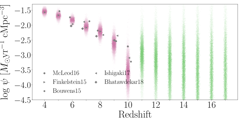
The simplicity of the model makes it comparably easy to extrapolate the result found in the previous section to higher, as of yet unobserved redshift bins. We do this in two ways: in the first approach we fix the quantity – halo mass relations to the parameter distributions found at the last included redshift ($z=10$ for the UVLF/GSMF, $z=5$ for the Type 1 AGN BHMF, $z=7$ for the QLF) and only evolving the HMF, and secondly by linearly extrapolating the quantity – halo mass relations to higher redshift. The extrapolation is done by drawing parameter samples from different redshift bins ($z=5-10$ for the GSMF/UVLF, $z=1-5$ for the Type 1 AGN BHMF and $z=2-7$ for the QLF), and calculating the linear trend using multivariate regression. The extrapolated number density functions are shown in Figure 14 (GSMF), Figure 15 (UVLF), Figure 16 (BHMF) and Figure 17 (QLF), with the bands covering the 68% credible regions. For all quantities, the extrapolation method leads to larger expected number densities compared with purely evolving the HMF. This is consistent with the results found in the previous subsection, which suggests the quantity – halo mass relations tend to increase in normalisation with redshift. We find that the extrapolation of our model is well in agreement with the recent estimates of the high-z UVLF from the JWST Early Data Release by Harikane et al. (2022) and Donnan et al. (2022).

From the linearly extrapolated parameter samples we also calculate the stellar mass density and other integrated quantities (shown in green in Figure 12, see Section 5.1), which show a continued decrease with increasing redshift despite the inferred increases in the relation between galaxy and halo properties, which lead to the larger expected number densities. This suggests that the decrease in the integrated densities is primarily driven by the evolution of the halo mass function, rather than changes in the quantity – halo mass relations.

Finally, in Table 3 and Table 4 we present an upper limit on the expected number of galaxies detected in the rest-frame UV for the Euclid deep field and JWST CEERS, Cosmos-Web, JADES and PRIMER surveys, based on our modelled UV luminosity function. We calculate the expected number of galaxies by integrating the UV luminosity function up to the reported $5\sigma$ depths (van Mierlo et al., 2021; Casey et al., 2022) and for redshift bins $\Delta z=1$. The upper limits are given by the 95th percentile of expected number of objects calculated from the model UVLFs shown in Figure 4 and Figure 15. Based on our estimation Euclid will be able to detect thousands of galaxies at $z\sim 5$, and some of the brightest galaxies up to $z\sim 11$. Across the different JWST surveys, dozens to hundreds of galaxies can be expected at $z>10$ including fainter galaxies representative down to $\mathcal{M}_{\mathrm{UV}}\approx 20$ at $z=15$. This will be further enhanced by JWST lensing surveys like GLASS (Roberts-Borsani et al., 2022), which we have not considered in our calculations.

6 Conclusion

We present an empirical model for the co-evolution of galaxies, SMBHs and dark matter halos by connecting the evolution of the halo mass function with prescriptions for baryonic physics. The model is fully analytical and computationally simple, which makes a full Bayesian treatment feasible. We show that this simple prescription is able to reproduce the observed galaxy stellar mass function, galaxy UV luminosity function, active black hole mass function and quasar bolometric luminosity function up to $z=10$, is able to link different observable properties to one another and makes predictions for quantities at weakly constrained or unobserved redshift.

The strength of this modelling approach lies in with which model parameter can be adjusted and physically interpreted. We show that the by calibrating our baryonic parametrizations to the observed number densities of the different physical quantities, we are to qualitatively reproduce the observed relations between these quantities. In particular, we are able to reproduce the slope of the UV luminosity – stellar mass relation, as well as the SMBH mass - galaxy stellar mass relation. Both of these relations have a systematic offset compared with observations, which are able to relate to model assumption. In particular, the former is likely caused by the assumption that observable properties and halo masses are connected uniquely, while the later can be explained by the fact that we do not explicitly model the duty cycles and active fraction of black holes. We discuss a potential avenue to include the effect of scatter in Appendix B. The model is further able to reproduce expected black hole mass distribution of a sample of Type 1 AGN, only by calibrating the model quasar luminosity function to observations.

Using the model, we are able to disentangle the effects of dark matter structure evolution and baryonic physics on the evolution of the observed galaxy properties, and are in particular able to study the evolution of the relation between dark matter halo mass and the baryonic properties. Key results are

1. Within uncertainties, the stellar mass – halo mass relation is consistent with an unevolving low mass slope up to $z=10$ and an unevolving high mass slope up to at least $z=2$. The main evolution takes place in the overall normalisation which increases with redshift, as well as an increase in feedback turnover-mass, which increases from $\sim 10^{12}M_{\odot}$ to $\sim 10^{12.4}M_{\odot}$ between $z=0$ and $z=2$.

2. Similarly, the UV luminosity – halo mass relation has an unevolving faint end slope between $z=2$-$10$ and an unevolving bright end slope at least for $z=2$-$4$. The overall normalisation increases with redshift, while the feedback turnover-mass stays constant at $\sim 10^{11.8}M_{\odot}$ between $z=2$-$4$. At $z<2$, data-related issues makes us unable to make reliable statements.

3. The observed quasar luminosity function can be reproduced up to $z=7$ with an redshift- and halo mass-independent Eddington rate distribution function.

The model is able to reproduce the observed stellar mass density for $z=1-9$ and observed star-formation rate density $z=4-10$, and produces a self-consistent with in the evolution of the stellar mass density when calculated directly and inferred from the star-formation rate. The model that the stellar mass density, star-formation rate density, black hole mass density and bolometric luminosity density are all decreasing for $z>3$ in a near log-linear fashion.

Based on these results, we present predictions on the number densities for redshift beyond the ones used for calibration by linearly extrapolating the calibrated baryonic parametrizations. Direct comparison of our prediction for the UVLF and Early Science Release for the JWST show that the predictions seem to be reasonable. Using these extrapolations, we are able to present upper limits on the expected number of objects for scheduled JWST (Table 3) and Euclid (Table 4) surveys.

In conclusion, we have shown that our simple empirical model is able to faithfully reproduce the observed evolution in galaxy and SMBH properties, and has the predictive power to make qualitative as well as quantitative statements about the interrelation of these properties and their evolution beyond the observations used to constrain the model. Conceptual and empirical models therefore provide an fast, easy, interpretable and adaptable framework for studying galaxy evolution, which can be use complementary to more comprehensive and computationally expensive models.

Figure 14: Extrapolated Galaxy Stellar Mass Function: The predicted GSMF is calculated by extrapolating the stellar mass – halo mass relation to the redshift in question and evolving the HMF (green), and by fixing the stellar mass – halo mass relation to the distribution at $z=10$ and only evolving the HMF(grey). The purple band is the last GSMF constrained by data. The shown bands correspond to the 68% credible regions.

Figure 15: Extrapolated Galaxy UV Luminosity Functions: Similar to Figure 14. The orange data points correspond to the estimates obtained from the JWST early data release estimated by Harikane et al. (2022) and Donnan et al. (2022).

Figure 16: Extrapolated Type 1 Active Black Hole Mass Functions: Similar to Figure 14.

Figure 17: Extrapolated Quasar Luminosity Functions: Similar to Figure 14.

Data Availability

The code, data used for calibration and posterior parameter distributions obtained from the MCMC sampling can be accessed under https://doi.org/10.5281/zenodo.7552484.

Appendix A The Halo Mass Function

Compared to the evolution of galaxies and baryonic matter in general, the formation and evolution of dark matter halos is a well-understood process, due to the comparably simple physics involved in the process. The halo mass function describes the distribution of dark matter halo masses across cosmic history and redshift $z$. If $\diff{n}{\log M_{\mathrm{h}}}$ denotes the number density $\operatorname{d\!}n$ of halos (per comoving Mpc) per infinitesimal mass bin $\operatorname{d\!}\log M_{\mathrm{h}}$, this quantity can be expressed as

$$\phi(M_{\mathrm{h}})=\diff{n}{\log M_{\mathrm{h}}}(M_{\mathrm{h}},z)=\frac{\overline{\rho}}{M_{\mathrm{h}}}f\left(\nu(M_{\mathrm{h}},z)\right)\left|\diff{\log\nu(M_{\mathrm{h}},z)}{\log M_{\mathrm{h}}}\right|,$$ (21)

Integration over $M_{\mathrm{h}}$, yields the total number density of halos in the mass range $[M_{1},M_{2}]$ at redshift z,

$$n(z)\bigg{|}_{M_{1}}^{M_{2}}=\int_{M_{1}}^{M_{2}}\frac{\overline{\rho}}{M_{\mathrm{h}}^{2}}f\left(\nu(M_{\mathrm{h}},z)\right)\left|\diff{\log\nu(M_{\mathrm{h}},z)}{\log M_{\mathrm{h}}}\right|\operatorname{d\!}M_{\mathrm{h}}.$$ (22)

Here, $\overline{\rho}$ is the comoving mean matter density and $\nu$ is defined by $\nu(M_{\mathrm{h}},z)=\frac{\delta^{2}_{\mathrm{c}}(z)}{\sigma^{2}(M_{\mathrm{h}},z)}$, where $\delta_{\mathrm{c}}(z)$ critical overdensity needed for the collapse of a halo and $\sigma^{2}(M_{\mathrm{h}},z)$ is the mass variance of the smoothed overdensity field (see e.g. Mo et al. (2010) for more details). Finally, the function $f(\nu)$ is called the multiplicity function and is given by

$$f(\nu)=C\left(1+\frac{1}{\nu^{\prime p}}\right)\left(\frac{\nu^{\prime}}{2\pi}\right)^{\nicefrac{{1}}{{2}}}e^{\nicefrac{{-\nu^{\prime}}}{{2}}},$$ (23)

where $\nu^{\prime}=a\nu$. (It is common in the literature to define a function $\widetilde{f}(\nu)$ instead, with $f(\nu)=\nu\widetilde{f}(\nu)$.) The parameters $(a,p,C)$ define the high mass cutoff, the shape at lower masses, and the normalisation of the curve, respectively (Sheth et al. 2001; Despali et al. 2015). These parameters can be estimated in various ways from theoretical considerations (Press & Schechter 1974; Sheth et al. 2001) or numerical simulations (Tinker et al. 2008; Despali et al. 2015). Though there has been much debate (Tinker et al. 2008; Courtin et al. 2010), it is assumed that the functional form and parameters $(a,p,A)$ of the multiplicity function are to a good approximation universal, meaning they are independent of redshift and specific cosmology (Despali et al. 2015). Discussions are still ongoing how much the idea of universality can be extended, and to what degree universality holds (Bocquet et al. 2015, 2020; Diemer 2020). Nonetheless, mass functions that are well described by Equation 23, and even the simple analytical expression such as the Press-Schechter (Press & Schechter 1974) and extended Press-Schechter (Bond et al. 1991; Sheth et al. 2001) formalisms seem to be good first-order approximations, especially at low to medium redshift. For our quantitative analysis, we have used the extended Press-Schechter HMF for ellipsoidal collapse given by Sheth et al. (2001). They derive a HMF of the form given by Equation 23 with the parameter set $(a,p,C)=(0.84,0.3,0.644)$. For many $\Lambda$CDM simulations, the extended Press-Schechter halo mass function yields a good approximation of the HMFs derived from numerical simulations up to $z\approx 15-20$.

Appendix B The Effect of Scatter

The focus of this work is on reproducing average relations between physical quantities, using the simplifying assumption that the observables and halo masses are linked by a one-to-one relation given by Equation 2. In reality however, environmental effects, the inherent stochastic nature of baryonic processes lead to a scatter in this relation, this means each halo mass will have an associated distribution for every observable quantities. As described in Section 2.3.2 for the Eddington ratios, large scatter in primary quantities can have striking effects on the number statistics and need to be included in order for the model to be able to match observations.

To include these effects in a systematic manner, it helps to recast the model as we have described in Section 2.1 in the language of probability distributions. The HMF, if normalised to unity (where we can introduce a low mass cutoff in case that the integral diverges), constitutes the probability density function (PDF) of halo masses in a given cosmic volume, i.e.

$$f_{M_{\mathrm{h}}}(m_{\mathrm{h}})=\frac{\phi(m_{\mathrm{h}})}{N},\quad\text{where}\quad N=\int_{m_{\mathrm{min}}}^{\infty}\phi(m_{\mathrm{h}})\operatorname{d\!}m_{\mathrm{h}}$$ (24)

is the total number of halos in the volume. The PDF $f_{Q}(q)$ for the observable $q$ is then obtained by a simple change of variables using Equation 2. To include scatter, rather than performing a change of variables we define a joint probability distribution,

$$f_{Q,M_{\mathrm{h}}}(q,m_{\mathrm{h}})=f_{Q|M_{\mathrm{h}}}\left(q|M_{\mathrm{h}}=m_{\mathrm{h}}\right)\cdot f_{M_{\mathrm{h}}}(m_{\mathrm{h}}),$$ (25)

where we now treat $Q$ and $M_{\mathrm{h}}$ as random variables. The conditional probability $f_{Q|M_{\mathrm{h}}}(q|M_{\mathrm{h}}=m_{\mathrm{h}})$ of $q$ with respect to $m_{\mathrm{h}}$ describes the the distribution of the quantity $Q$ at a fixed halo mass $M_{\mathrm{h}}=m_{\mathrm{h}}$, i.e. the scatter in the relation we want to include. The marginal distribution for the $Q$ is given by

$$f_{Q}(q) =\int_{m_{\mathrm{min}}}^{\infty}f_{Q,M_{\mathrm{h}}}(q,m_{\mathrm{h}})\operatorname{d\!}m_{\mathrm{h}}$$

$$=\int_{m_{\mathrm{min}}}^{\infty}f_{Q|M_{\mathrm{h}}}(q|M_{\mathrm{h}}=m_{\mathrm{h}})\cdot f_{M_{\mathrm{h}}}(m_{\mathrm{h}})\operatorname{d\!}m_{\mathrm{h}},$$ (26)

and the number density of the observable is $\phi(q)=N\cdot f_{Q}(q)$.

As an example, a scatter-free relation between observable and halo mass as described by Equation 2 would be described by a conditional probability of the form

$$f_{Q|M_{\mathrm{h}}}(q|M_{\mathrm{h}}=m_{\mathrm{h}})=\delta\left(q-\mathcal{Q}(m_{\mathrm{h}})\right),$$ (27)

with $\delta$ being the Dirac delta distribution. The marginal probability for $Q$ in this case is given by

$$f_{Q}(q) =\int_{m_{\mathrm{min}}}^{\infty}f_{Q,M_{\mathrm{h}}}(q,m_{\mathrm{h}})\operatorname{d\!}m_{\mathrm{h}}$$

$$=\int_{m_{\mathrm{min}}}^{\infty}\delta\left(q-\mathcal{Q}(m_{\mathrm{h}})\right)\cdot f_{M_{\mathrm{h}}}(m_{\mathrm{h}})\operatorname{d\!}m_{\mathrm{h}}$$

$$=\int_{m_{\mathrm{min}}}^{\infty}\frac{\delta(m_{\mathrm{h}}-m_{\mathrm{h}}^{*})}{|\mathcal{Q}^{\prime}(m_{\mathrm{h}}^{*})|}\cdot f_{M_{\mathrm{h}}}(m_{\mathrm{h}})\operatorname{d\!}m_{\mathrm{h}}$$

$$=\frac{f_{M_{\mathrm{h}}}(m_{\mathrm{h}}^{*})}{|\mathcal{Q}^{\prime}(m_{\mathrm{h}}^{*})|},$$ (28)

which recovers Equation 3 obtained in the original approach. Here, $m_{\mathrm{h}}^{*}$ is the halo mass that solves Equation 2 for a given $q$ and we make use of the function composition property of the delta distribution. To include scatter, we could e.g. assume the marginal distribution to be a Gaussian with a central value given by Equation 2 and a halo mass-independent variance $\sigma^{2}$,

$$f_{Q|M_{\mathrm{h}}}(q|M_{\mathrm{h}}=m_{\mathrm{h}})=\mathcal{N}\left(\mathcal{Q}(m_{\mathrm{h}}),\sigma^{2}\right).$$ (29)

This generalized approach has a number of advantages beside the ability to include scatter. For one, there is no need for the function $\mathcal{Q}$ to be invertible anymore, since multiple halo masses can be assigned to the same observable value. Further, it is easy to calculate higher moments of the various quantities, enabling the study of the scatter and skewness of the distributions rather than just mean relations. To study the interrelation of observables, one can construct the probability distributions of one quantity with respect to another, i.e.

$$p(q_{1}|q_{2})=\int_{m_{\mathrm{min}}}^{\infty}f_{Q_{1}|M_{\mathrm{h}}}(q_{1}|m_{\mathrm{h}})\cdot f_{M_{\mathrm{h}}|Q_{2}}(m_{\mathrm{h}}|q_{2})\operatorname{d\!}m_{\mathrm{h}},$$ (30)

where $f_{M_{\mathrm{h}}|Q_{2}}(m_{\mathrm{h}}|q_{2})$ is given by

$$f_{M_{\mathrm{h}}|Q_{2}}(m_{\mathrm{h}}|q_{2})=\frac{f_{Q_{2},M_{\mathrm{h}}}(q_{2},m_{\mathrm{h}})}{f_{Q_{2}}(q_{2})}.$$ (31)

Figure 18: Influence of scatter on the stellar mass – UV luminosity relation: Shown are the conditional probability distributions of the galaxy stellar mass for a fixed UV magnitude $\mathcal{M}_{\mathrm{UV}}=-20$ when including scatter in the stellar mass – halo mass and UV luminosity – halo mass relations, calculated using Equation 30 for a fixed set of model parameter. The grey line shows the probability distribution when assuming $\log M_{\star}$ and $\log L_{\mathrm{UV}}$ are distributed according to a Gaussian distribution with $\sigma_{M_{\star}}=0.05$ and $\sigma_{L_{\mathrm{UV}}}=0.25$. The purple line assumes a skewnormal distribution (a generalisation of the normal distribution that allows for non-zero skewness) for $L_{\mathrm{UV}}$ with a skewness parameter $\alpha=-40$. All distributions have a median given by Equation 2. The black vertical line shows the value of $M_{\star}$ calculated without assuming scatter. Evidently, the scatter influences the location and shape of the distributions, the skewed case produces a distributions that more closely matches the observations shown in Figure 7.

Figure 19: Influence of scatter on the GSMF: Shown are the modelled stellar mass functions for a fixed set of model parameter at $z=0$. The grey line shows the GSMF calculated assuming a one-to-one relationship between the quantities and halo masses, as done throughout this paper. The purple lines show the GSMF calculated using the same parameter but adding a Gaussian scatter to the stellar mass – halo mass relation with different variances. The high mass slope is strongly sensitive to the amount of scatter, while the normalisation is weakly affected and low mass slope unaffected.

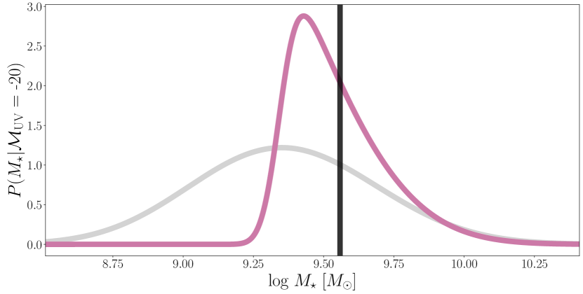
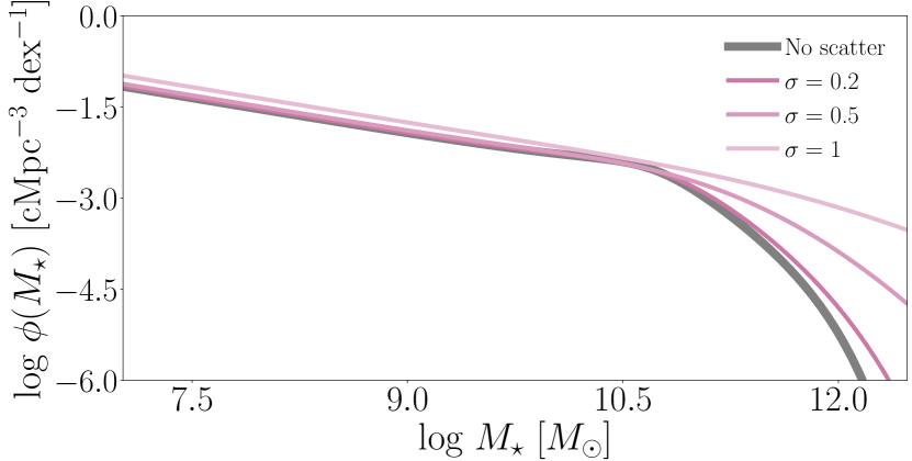
Appendix C Parameter Table

Table 5 and Table 6 show the median parameters values obtained by MCMC sampling of the posterior distribution, as well as the range that encapsulates the 95% credible interval.

Table 5: Reference list for the galaxy property-related parameter: Given are the median parameter values and uncertainties that cover the 95% credible interval. Note that the median values do not necessarily correspond to the most likely parameter (as defined by the MAP estimator). For calculations, the provided MCMC chains should be used. For $z>3$ ($M_{\star}$) and $z>5$ ($L_{\mathrm{UV}}$), we marginalise over $M_{\mathrm{c}}$ and $\delta$ in our analysis, so that no values are given.

$z$	$\log M_{\mathrm{c}}^{\star}$	$\log A_{\star}$	$\gamma_{\star}$	$\delta_{\star}$	$\log M_{\mathrm{c}}^{\mathrm{UV}}$	$\log A_{\mathrm{UV}}$	$\gamma_{\mathrm{UV}}$	$\delta_{\mathrm{UV}}$
0	$12.1_{-0.05}^{+0.06}$	$-1.69_{-0.04}^{+0.04}$	$1.32_{-0.1}^{+0.1}$	$0.43_{-0.02}^{+0.02}$	$11.66_{-0.35}^{+0.39}$	$15.44_{-0.21}^{+0.18}$	$1.67_{-0.76}^{+1.57}$	$0.36_{-0.19}^{+0.14}$
1	$12.24_{-0.07}^{+0.07}$	$-1.72_{-0.04}^{+0.04}$	$1.45_{-0.15}^{+0.16}$	$0.44_{-0.04}^{+0.03}$	$11.5_{-0.15}^{+0.19}$	$16.01_{-0.12}^{+0.11}$	$2.34_{-1.18}^{+1.46}$	$0.23_{-0.12}^{+0.12}$
2	$12.4_{-0.17}^{+0.17}$	$-1.72_{-0.09}^{+0.07}$	$1.4_{-0.25}^{+0.34}$	$0.3_{-0.13}^{+0.12}$	$11.39_{-0.17}^{+0.17}$	$16.65_{-0.06}^{+0.05}$	$1.17_{-0.25}^{+0.32}$	$0.33_{-0.05}^{+0.05}$
3		$-1.27_{-0.35}^{+0.63}$	$0.61_{-0.13}^{+0.36}$		$11.44_{-0.24}^{+0.3}$	$16.99_{-0.11}^{+0.08}$	$1.19_{-0.39}^{+0.49}$	$0.3_{-0.11}^{+0.11}$
4		$-1.61_{-0.22}^{+0.72}$	$0.89_{-0.4}^{+0.59}$		$11.24_{-0.34}^{+0.91}$	$17.08_{-0.14}^{+0.22}$	$1.19_{-0.67}^{+0.94}$	$0.08_{-0.08}^{+0.26}$
5		$-1.11_{-0.3}^{+0.64}$	$1.16_{-0.33}^{+0.56}$			$17.6_{-0.31}^{+0.66}$	$0.44_{-0.18}^{+0.59}$
6		$-0.8_{-0.39}^{+0.39}$	$0.88_{-0.16}^{+0.21}$			$17.9_{-0.36}^{+0.64}$	$0.42_{-0.11}^{+0.2}$
7		$-1.2_{-0.3}^{+0.69}$	$1.25_{-0.4}^{+0.62}$			$18.31_{-0.6}^{+1.03}$	$0.53_{-0.17}^{+0.27}$
8		$-0.92_{-0.6}^{+0.49}$	$1.12_{-0.43}^{+0.84}$			$18.52_{-0.79}^{+1.51}$	$0.64_{-0.24}^{+0.52}$
9		$-1.34_{-0.65}^{+0.9}$	$1.52_{-0.89}^{+1.99}$			$18.76_{-0.8}^{+1.66}$	$0.61_{-0.25}^{+0.52}$
10		$-1.63_{-1.0}^{+1.15}$	$1.02_{-0.89}^{+2.64}$			$19.25_{-1.49}^{+4.12}$	$1.1_{-0.61}^{+2.1}$

Table 6: Reference list for the SMBH property-related parameter: Same as Table 5, but the the SMBH parameter. The black hole mass function related parameter ($B$, $\eta$ are estimated up to $z=5$. For the quasar luminosity function, the Eddington ratio-related parameter are fixed to the MAP estimator at $z=0$.

$z$	$\log B$	$\eta$	$\log C$	$\theta$	$\log\lambda_{\mathrm{c}}$	$\rho$
0	$4.17_{-1.48}^{+1.13}$	$1.5_{-0.35}^{+0.48}$	$40.08_{-1.13}^{+0.62}$	$2.23_{-0.25}^{+0.42}$	$-2.35_{-0.55}^{+0.43}$	$1.44_{-0.05}^{+0.05}$
1	$6.23_{-1.85}^{+0.76}$	$1.56_{-0.47}^{+1.53}$	$40.77_{-0.12}^{+0.12}$	$2.88_{-0.06}^{+0.05}$
2	$6.03_{-1.5}^{+0.76}$	$2.01_{-0.41}^{+0.81}$	$42.5_{-0.11}^{+0.11}$	$3.24_{-0.07}^{+0.07}$
3	$6.73_{-3.93}^{+1.19}$	$2.21_{-0.78}^{+2.73}$	$43.52_{-0.17}^{+0.17}$	$3.4_{-0.14}^{+0.14}$
4	$6.35_{-4.79}^{+1.42}$	$3.22_{-1.27}^{+4.62}$	$43.06_{-0.27}^{+0.25}$	$4.73_{-0.23}^{+0.25}$
5	$2.78_{-2.67}^{+5.56}$	$10.95_{-8.4}^{+7.74}$	$44.72_{-0.97}^{+0.78}$	$3.99_{-1.57}^{+1.2}$
6			$44.97_{-0.98}^{+0.7}$	$4.83_{-1.83}^{+1.57}$
7			$46.23_{-1.29}^{+0.39}$	$4.49_{-2.28}^{+3.29}$