DehazeNeRF: Multiple Image Haze Removal and 3D Shape Reconstruction using Neural Radiance Fields

Abstract

Neural radiance fields (NeRFs) have demonstrated state-of-the-art performance for 3D computer vision tasks, including novel view synthesis and 3D shape reconstruction. Yet, these methods fail in adverse weather conditions that are crucial for applications such as autonomous driving. To address this challenge, we introduce DehazeNeRF as a framework that robustly operates in hazy conditions. DehazeNeRF extends the volume rendering equation by physically realistic terms that model atmospheric scattering. These act as inductive network biases in our pipeline and, together with several regularization strategies, allow DehazeNeRF to demonstrate successful multi-view haze removal, novel view synthesis, and 3D shape reconstruction where existing approaches fail.

1 Introduction

Neural radiance fields (NeRFs) [46] have emerged as a powerful approach to solving 3D computer vision problems, such as novel view synthesis and 3D reconstruction [64]. Existing NeRF approaches are successful in many scenarios, but they fail to accurately reconstruct the geometry and appearance of a 3D scene in adverse weather conditions such as haze (see Fig. 6). This poses a critical limiting factor for many real-life applications, including autonomous driving among others.

The problem of applying NeRF to hazy input images is the ambiguity between light-reflecting solid surfaces and light-scattering atmospheric particles in free space – both are interchangeably modeled as a light-emitting volume by NeRF and cannot be disambiguated. Most state-of-the-art dehazing methods adopt feedforward neural networks [62, 1], but applying these to the input views as a preprocessing step to standard NeRFs leads to poor reconstruction results, in part because these techniques tend to overfit to the training data and generalize poorly to real-world data [55, 61].

Figure 1: Given a set of posed hazy images, our method estimates the haze-free scene using a neural radiance field that includes physically based terms for scattering. Here, we show results of an experimentally captured scene.

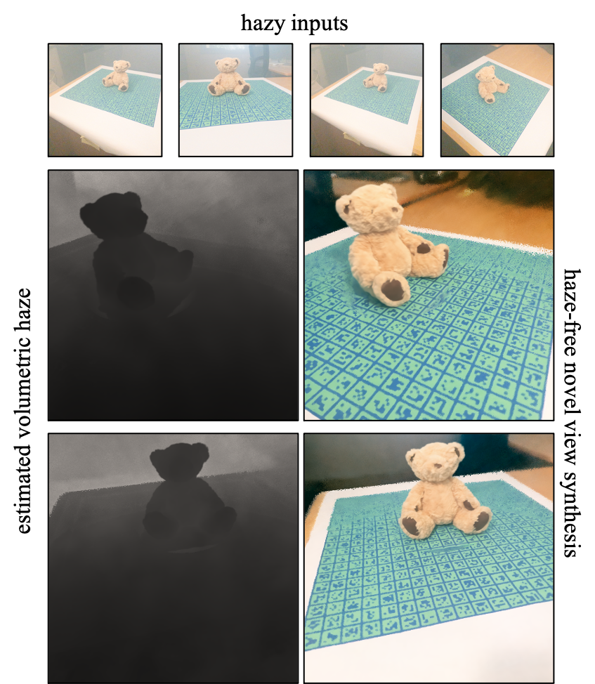
To address this limitation, we develop a differentiable physically based 3D haze model that seamlessly integrates into the volume rendering framework used by NeRF. In the absence of scattering, our model is equivalent to NeRF. For the inverse problem of estimating the scene parameters from multiple posed input views, our 3D haze model is used in conjunction with several regularization strategies that disentangle solid object surfaces from scattering volumetric particles. Our proposed framework jointly learns the 3D shape and haze components of a scene and allows for significantly improved and multi-view-consistent novel view synthesis as well as more accurate 3D shape reconstruction compared to previous work. Our approach does not require large collections of paired hazy-clear images and it circumvents the sim2real gap of data-driven dehazing methods by building an inductive bias based on the physics of scattering into the network architecture.

Specifically, our contributions include:

• extending the volume rendering equation of NeRF by a physically based 3D haze image formation model to accurately model the in-scattering phenomenon prevalent in hazy conditions;

• introducing multiple physically inspired inductive biases as well as optimization regularizers to effectively disambiguate the surface appearance thus achieving accurate clear-view appearance and geometry reconstruction using only hazy image as inputs.

We demonstrate state-of-the-art results using simulation and experimental data for 3D multi-view construction and novel view synthesis under hazy condition. Code and data will be made available for research purposes.

2 Related Work

DehazeNeRF integrates knowledge from several areas of research. We briefly review these next.

2.1 3D Scene Reconstruction with NeRF

Neural radiance fields (NeRFs) [46] were introduced for novel view synthesis applications. By combining differentiable volumetric rendering from classic computer graphics and learnable radiance field, NeRF can jointly optimize for the geometry and appearance of a static 3D scene from posed RGB images. As the performance of the original NeRF noticeably deteriorates under imperfect capturing conditions, much research has investigated the robustness of NeRF under a variety of challenging conditions, such as blur [40], noise [52], reflection [19], low resolution [69], low dynamic range [22, 45], and occlusion [41, 8]. In this paper, we address haze, an unexplored yet common scenario in real-life captures. Our method leverages a scattering-aware rendering equation to model the haze phenomenon and disambiguate the surface and haze by using physically inspired inductive biases. Among those, we adopt a surface-like density field parameterization [71] to encourage solid geometry, although other surface priors may be equally applied in our method [49, 75, 71, 50].

2.2 Dehazing

We provide a brief summary of existing dehazing methods and refer to [62] for a comprehensive review. Early works aim to design strong priors to recover the transmission map, global atmospheric light, and scene radiance [83, 5, 13, 20, 2], thus they struggle on scenes where these priors do not hold [39]. More recently, data-driven methods [39, 7, 10, 43, 79, 18] achieve better quality using deep learning and large datasets [32], but have difficulty generalizing to images in the real world [61]. More related to our work are multi-image dehazing methods, which exploit the consistency between neighboring frames. Similar to single-image approaches, multi-image approaches can be divided into prior-based or data-driven categories. The former adds photo-consistency regularization between neighboring frames using jointly estimated or known depth [80, 33, 14], while the latter achieves more temporal stability by fusing features from a small number of neighboring frames [57, 72, 82]. Yet both approaches are subject to the aforementioned problems exhibited in the single-image scenario. Furthermore, none of these dehazing methods estimates a holistic 3D structure, and therefore they are not directly applicable to novel view synthesis.

Estimating Scattering Coefficients.

In addition to estimating the 3D geometry and haze-free appearance in novel views, we also jointly optimize for the scattering coefficient. Prior work mainly computes the scattering coefficient based on handcrafted priors such as average saturation [17], dark channel mean [9], polarization [58], and gamma correction [26]. In data-driven approaches, the scattering coefficient can be estimated explicitly as an intermediary output [74, 68]. Our method directly estimates the scattering coefficient in 3D, while at the same time utilizing 2D priors such as dark channel mean to address the ambiguity with other physical properties such as airlight.

Seeing through Scattering Media.

Various methods have been developed to solve the challenging problem of imaging through and within scattering media. These methods can be classified as interference of light, relying on ballistic photons, and being based on diffuse optical tomography. For methods based on interference of light, they leverage information in the speckle pattern to reconstruct the image [54, 29, 3] or adopt wavefront shaping to focus light through or within scattering media [21, 66]. On the other hand, ballistic photons can avoid scattered photons since they can travel through a medium without scattering and can be isolated by adopting time-gating [56, 70], coherence-gating [23, 11], or coherent probing and detection of a target at different illumination angles [28]. The last class is to adopt non-line-of-sight imaging techniques [67, 38, 51, 36, 12, 37, 77] or diffuse optical tomography [4, 15, 35] to recover objects by modeling and inverting scattering of light explicitly. However, these methods all require exotic hardware setups, which are usually expensive, and are limited to some scenarios such as long propagation distance of light or scale of resolution. Our approach removes the scattering effect using inverse rendering, requiring only a set of RGB images of a hazy scene. Similar principles have been explored in concurrent and independent work [31] for underwater scene reconstruction.

3 Method

Our method, DehazeNeRF, extends the volume rendering equation to accurately reconstruct the geometry and appearance robust to hazy conditions. Our key idea is to introduce a series of important biases in the network architecture along with regularizers in the loss function that together underpin physically based scattering phenomena.

3.1 Preliminary on Neural Radiance Fields

Neural Radiance Fields (NeRFs) [46] map a 3D sample point $\mathbf{p}$ into a color $\mathbf{c}$ and volume density $\sigma$. Considering only emission from classic volume rendering [27, 63], the expected color ${C}(\mathbf{r})$ of a camera ray $\mathbf{r}(t)=\mathbf{o}+t\mathbf{d}$ with the near and far boundary $t_{n}$ and $t_{f}$ can be written as

$${C}(\mathbf{r},\mathbf{d})=\int_{t_{n}}^{t_{f}}T(t)\sigma(\mathbf{r}(t))c(\mathbf{r}(t),\mathbf{d})\ dt\;\textrm{with}$$ (1)

$$T(t)=\mathrm{exp}\left(-\int_{t_{n}}^{t}\sigma(\mathbf{r}(t^{\prime}))\ dt^{\prime}\right),$$ (2)

where $T(t)$ is the accumulated transmittance between the ray section $t_{n}$ to $t$. The predicted pixel value is then compared to the ground truth $\widehat{C}(\mathbf{r},\mathbf{d})$ for optimization.

3.2 3D Haze Formation

To address the 3D dehazing problem, we propose an alternative rendering equation to the image formation model. We start from the radiative transfer equation (RTE) [6, 65], which describes the behavior of light in a medium that absorbs, scatters and emits radiation. Assuming, a ray $\mathbf{r}\left(t\right)=\mathbf{o}+t\mathbf{d}$ hits a surface point at $\mathbf{r}\left(t_{0}\right)$, the incident radiance at the near image plane $t_{n}$ can be divided into three parts [53]:

$$C(\mathbf{r},\mathbf{d}) =C_{\textrm{emission}}(\mathbf{r})+C_{\textrm{surface}}(\mathbf{r})+C_{\textrm{in-scattering}}(\mathbf{r})$$

$$C_{\textrm{emission}}(\mathbf{r},\mathbf{d}) =\int_{t_{n}}^{t_{0}}\epsilon\left(\mathbf{r}\left(t\right),\mathbf{d}\right)T_{\sigma_{t}}\left(t\right)dt$$

$$C_{\textrm{surface}}(\mathbf{r},\mathbf{d}) =C_{e}\left(\mathbf{r}\left(t_{0}\right),\mathbf{d}\right)T_{\sigma_{t}}\left(t_{0}\right)$$

$$C_{\textrm{in-scattering}}(\mathbf{r},\mathbf{d}) =\int_{t_{n}}^{t_{0}}c_{\textrm{s}}\left(\mathbf{r}\left(t\right),\mathbf{d}\right)\sigma_{s}\left(\mathbf{r}\left(t\right)\right)T_{\sigma_{t}}\left(t\right)dt,$$

where $\epsilon$ is the emission, $C_{e}$ is the outgoing radiance at the surface intersection, $c_{\textrm{s}}\left(\mathbf{r}\left(t\right),\mathbf{d}\right)$ is the in-scattered light and $\sigma_{s}$ is the scattering coefficient. In particular, the transmittance here is computed from the attenuation coefficient $\sigma_{t}$, i.e., $T_{\sigma_{t}}\left(t\right)=\exp\left(-\int_{t_{n}}^{t}\sigma_{t}(t^{\prime})dt^{\prime}\right)$, where $\sigma_{t}=\sigma_{a}+\sigma_{s}$ including the absorption and out-scattering effect. For common haze formation, the participating particles are considered non-luminous [48], therefore we can drop the emission part, which leads to

$$\begin{split}C(\mathbf{r},\mathbf{d})={}&C_{e}(\mathbf{r}\left(t_{0}\right),\mathbf{d})T_{\sigma_{t}}\left(t_{0}\right)+\\ &\int_{t_{n}}^{t_{0}}c_{\textrm{s}}\left(\mathbf{r}\left(t\right),\mathbf{d}\right)\sigma_{s}\left(\mathbf{r}\left(t\right)\right)T_{\sigma_{t}}\left(t\right)dt.\end{split}$$ (3)

Following NeRF [46], we represent the surface as a continuous density field with emission $\epsilon\left(\mathbf{r}\left(t\right),\mathbf{d}\right)\coloneqq c\left(\mathbf{r}\left(t\right),\mathbf{d}\right)\sigma\left(\mathbf{r}\left(t\right)\right)$. Meanwhile, the absorption part in the attenuation $\sigma_{t}$ can be interpreted as the surface density $\sigma$, since the volume density $\sigma$ is equal to absorption coefficient $\sigma_{a}$ in that they both determine the probability of a photon or a ray terminating at a given location. As a result, we can write the rendering equation as

$$\begin{split}C(\mathbf{r},\mathbf{d})=&\underbrace{\int_{t_{n}}^{t_{0}}c(\mathbf{r}(t),\mathbf{d})\sigma(t)T_{\sigma+\sigma_{s}}\left(t\right)dt}_{C_{\textrm{Surface}}}+\\ &\underbrace{\int_{t_{n}}^{t_{0}}c_{s}(\mathbf{r}(t))\sigma_{s}(t)T_{\sigma+\sigma_{s}}\left(t\right)dt}_{C_{\textrm{Haze}}}.\end{split}$$ (4)

Eq. 4 formally disentangles the surface and haze, represented by $\left\{c,\sigma\right\}$ and $\left\{c_{s},\sigma_{s}\right\}$ respectively, in a principled manner. Once successfully optimized (see the next Section), the clear-view surfaces can be recovered using $\left\{c,\sigma\right\}$:

$$C(\mathbf{r},\mathbf{d})=\int_{t_{n}}^{t_{0}}c(\mathbf{r}(t),\mathbf{d})\sigma(t)T_{\sigma}\left(t\right)dt.$$ (5)

Figure 2: DehazeNeRF architecture. Given a set of hazy images, our method augments the existing NeRF pipeline (gray) with a haze module (yellow), which explicitly models the scattering phenomenon using atmospheric light and scattering coefficient. During training, we render the hazy reconstruction as a composition of surface and haze, which is compared to the input hazy images to optimize the learnable parameters (in green) jointly. During inference, we use the surface module (gray) to render clear views.

3.3 Haze-aware Neural Radiance Field

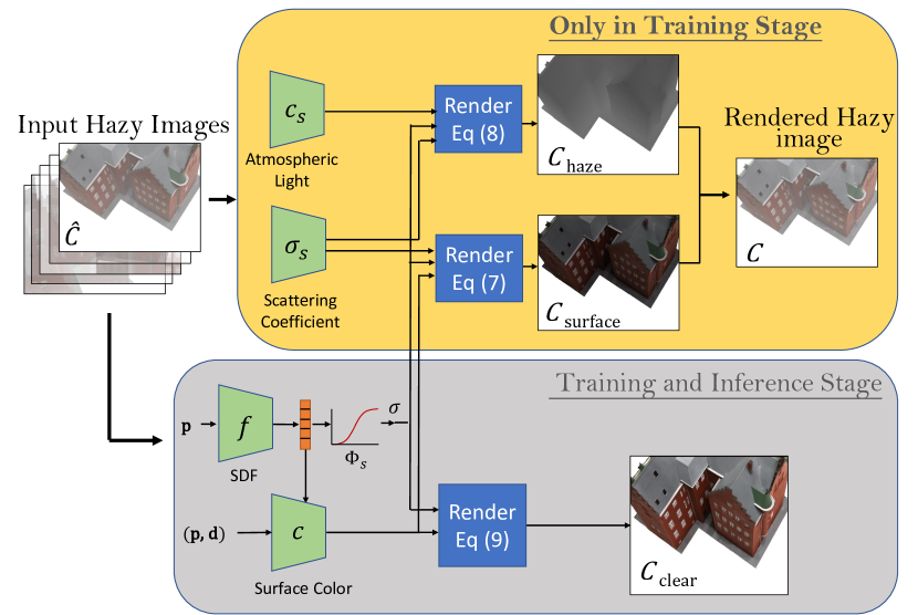
Given multiple images of a hazy scene, we aim to jointly optimize for the surface appearance and geometry, $\left\{c,\sigma\right\}$ as well as the haze’s scattering coefficient and in-scattered light (atmospheric light), $\left\{c_{s},\sigma_{s}\right\}$ based on the enhanced scattering-aware rendering equation Eq. 4. However, the effects of these variables are interdependent. In order to correctly disentangle them, our model adopts suitable architecture designs and training regularizers to capture the distinct physical properties of haze and surface. An overview of DehazeNeRF is illustrated in Fig. 2.

Architecture.

Now we introduce inductive biases to match the physical properties of haze and surface. For clarity, we highlight the quantities directly modeled by neural networks in green.

Modeling a Surface. Recall our goal is to learn the surface appearance and geometry, $\left\{c,\sigma\right\}$. Similar to previous works [46], we model the appearance ${\color[rgb]{0,0,0}\definecolor[named]{pgfstrokecolor}{rgb}{0,0,0}c}\left(\mathbf{p},\mathbf{d}\right)$ with an MLP, which takes the sample location $\mathbf{p}$ and viewing direction $\mathbf{d}$ as inputs. However, in order to encourage volume density $\sigma$ to form a well-defined solid surface, instead of directly learning the volume density, we adopt the reparameterization of the volume density using signed distance function (SDF), ${\color[rgb]{0,0,0}\definecolor[named]{pgfstrokecolor}{rgb}{0,0,0}f}\left(\mathbf{r}\left(t\right)\right)\in\mathbb{R}$, as proposed in NeuS [71, 73]. The modified surface volume density $\sigma\left(\mathbf{r}\left(t\right)\right)$, referred to as opaque density, can be parameterized as ${\color[rgb]{0,0,0}\definecolor[named]{pgfstrokecolor}{rgb}{0,0,0}f}\left(\mathbf{r}\left(t\right)\right)$:

$$\sigma\left(\mathbf{r}\left(t\right)\right)=s\left(\Phi_{s}\left({\color[rgb]{0,0,0}\definecolor[named]{pgfstrokecolor}{rgb}{0,0,0}f}\left(\mathbf{r}\left(t\right)\right)\right)-1\right)\nabla{\color[rgb]{0,0,0}\definecolor[named]{pgfstrokecolor}{rgb}{0,0,0}f}\left(\mathbf{r}\left(t\right)\right)\mathbf{d},$$ (6)

where $\Phi_{s}(x)$ is the sigmoid function $\Phi_{s}(x)=(1+e^{-sx})^{-1}$, whose derivative is a bell-shaped density function centered at 0 and has a learnable standard deviation of $\nicefrac{{1}}{{s}}$. We derive the discrete approximate following [46, 63]. It samples $n$ points $\left\{\mathbf{p}_{i}=\mathbf{o}+t_{n}\mathbf{d}|n=1,...,N,t_{n}<t_{n+1}\right\}$ along the ray. The approximate pixel color of the ray is computed based on quadrature rule [42], yielding

$$\begin{gathered}C_{\textrm{surface}}(\mathbf{r},\mathbf{d})=\sum_{n=1}^{N}\frac{\sigma^{n}}{\sigma_{t}^{n}}T_{t}^{n}\alpha_{t}^{n}{\color[rgb]{0,0,0}\definecolor[named]{pgfstrokecolor}{rgb}{0,0,0}c}^{n}\textrm{ with }T_{t}^{n}=\prod_{m=1}^{n-1}\left(1-\alpha_{t}^{m}\right),\end{gathered}$$ (8)

where $\alpha_{t}$ denotes the discrete $\alpha$-compositional weight defined as [71, 73]

where $\sigma_{t}^{n}=\sigma^{n}+{\color[rgb]{0,0,0}\definecolor[named]{pgfstrokecolor}{rgb}{0,0,0}\sigma_{s}}^{n}$ denotes the total attenuation at sample $n$, including the attenuation due to surface occlusion and the out-scattering.

Modeling Haze. We use a low-frequency prior to compute the scattering coefficient and atmospheric light, $\left\{c_{s},\sigma_{s}\right\}$, since these components usually vary slowly in a common hazy scenes [33]. In practice, we use a small band-limited MLP [34] for the scattering coefficient $\sigma_{s}$ to capture inhomogenous haze. Analogous to Eq. 8, the haze color can be approximated as

$$\begin{gathered}C_{\textrm{haze}}(\mathbf{r})=\sum_{n=1}^{N}\frac{{\color[rgb]{0,0,0}\definecolor[named]{pgfstrokecolor}{rgb}{0,0,0}\sigma_{s}}^{n}}{\sigma_{t}^{n}}T_{t}^{n}\alpha_{t}^{n}{\color[rgb]{0,0,0}\definecolor[named]{pgfstrokecolor}{rgb}{0,0,0}c_{s}}^{n}.\end{gathered}$$ (9)

During optimization, the color for an arbitrary input hazy image can be written as $C=C_{\textrm{surface}}+C_{\textrm{haze}}$. At test time, we can reconstruct the clear-view color by discretizing Eq. 5, namely:

$$C_{\textrm{clear}}\left(\mathbf{r},\mathbf{d}\right)=\sum_{n=1}^{N}T_{\sigma}^{n}\alpha^{n}{\color[rgb]{0,0,0}\definecolor[named]{pgfstrokecolor}{rgb}{0,0,0}c}^{n},$$ (10)

Optimization.

While the inductive biases separate the high-frequency surface appearance and geometry from the low-frequency color and density of the scattering medium, we introduce further regularizers to guide the optimization process to converge to more plausible clear-view geometry and color.

Koschmieder Consistency. Given an accurate depth map $D$, assuming globally constant scattering coefficient $\bar{\sigma}_{s}$ and airlight $\bar{c}_{s}$, the relation between a clear-view image $C_{\textrm{clear}}$ and the hazy image $C$ can be described by the Koschmieder law [24] as

This model is widely adopted as the basis for image-based single and multiview dehazing. The Koschmider model is an approximation of our rendering equation Eq. 4 under the assumption of spatially-invariant (i.e., homogeneous) scattering coefficient and an ideal surface

$$C_{\textrm{surface}}\left(\mathbf{r}\right) \approx C_{\textrm{clear}}(\mathbf{r})\exp(-\bar{\sigma}_{s}D(\mathbf{r}))=\tilde{C}_{\textrm{surface}}\left(\mathbf{r}\right)$$ (12)

$$C_{\textrm{haze}}\left(\mathbf{r}\right) \approx\bar{c}_{s}(1-\exp(-\bar{\sigma}_{s}D(\mathbf{r}))=\tilde{C}_{\textrm{haze}}\left(\mathbf{r}\right),$$ (13)

We promote this relation with

$$\mathcal{L}_{\textrm{2D}}=\left\|C_{\textrm{surface}}\left(\mathbf{r}\right)-\tilde{C}_{\textrm{surface}}\left(\mathbf{r}\right)\right\|_{1}$$ (14)

$$+ \left\|C_{\textrm{haze}}\left(\mathbf{r}\right)\!-\!\tilde{C}_{\textrm{haze}}\left(\mathbf{r}\right)\right\|_{1}\!\!+\!\left\|C\!-\!\tilde{C}_{\textrm{surface}}\left(\mathbf{r}\right)\!-\!\tilde{C}_{\textrm{haze}}\left(\mathbf{r}\right)\right\|_{1}\!,$$

where $\bar{\sigma}_{s}$ and $\bar{c}_{s}$ are the average over the samples on the ray, while the depth value $D\left(\mathbf{r}\right)$ is computed via the learned surface geometry [46, 78] by accumulating over ray-length over all the samples on a ray:

$$D\left(\mathbf{r}\right)=\sum_{n=1}^{N}T_{\sigma}^{n}\alpha^{n}t^{n}.$$ (15)

Color Prior. Without knowing the original image, the heavily attenuated color in the hazy image can be explained by the haze but also by a dull surface color. In order to reconstruct plausible clear-view colors, we adopt the popular 2D prior widely used in image-based dehazing methods, Dark Channel Prior (DCP) [20], which arises from the observation, that for most pixels in a natural haze-free image, the minimum of three color channels is close to zero. We apply this prior to the estimated clear image $C_{\textrm{clear}}$

$$DC(C_{\textrm{clear}})\left(\mathbf{x}\right) =\underset{\mathbf{y}\in\Omega\left(\mathbf{x}\right)}{\min}\left(\underset{c\in\left\{r,g,b\right\}}{\min}C_{\textrm{clear}}^{c}\left(\mathbf{y}\right)\right),$$ (16)

$$\mathcal{L}_{\textrm{dcp}} =\frac{1}{K}\sum\limits_{k=1}^{K}\|DC\left(C_{\textrm{clear}}\right)\|_{1}.$$ (17)

3.4 Implementation Details

We adopt the same setting as that in HF-NeuS [71] wherever possible. This includes the MLPs for the surface SDF, ${\color[rgb]{0,0,0}\definecolor[named]{pgfstrokecolor}{rgb}{0,0,0}f}$ and the view-dependent surface color, ${\color[rgb]{0,0,0}\definecolor[named]{pgfstrokecolor}{rgb}{0,0,0}c}$, as well as the sampling strategy, the background composition, and learning rate schedule.

Loss.

Our loss is composed of several terms:

$$\mathcal{L}=\mathcal{L}_{\textrm{color}}+\lambda\mathcal{L}_{\textrm{eikonal}}+\alpha\mathcal{L}_{\textrm{dcp}}+\beta\mathcal{L}_{\textrm{2D}},$$ (18)

where $\mathcal{L}_{\textrm{dcp}}$ and $\mathcal{L}_{\textrm{2D}}$ are the regularizations introduced in Sec. 3.3, while the photo-consistency loss, $\mathcal{L}_{\textrm{color}}$, is the standard NeRF loss, and the eikonal loss, $\mathcal{L}_{\textrm{eikonal}}$, is commonly used to regularize SDF [16],

$$\mathcal{L}_{\textrm{color}} =\frac{1}{K}\sum_{k=1}^{K}\left\|\widehat{C}_{k}(\mathbf{r},\mathbf{d})-C_{k}(\mathbf{r},\mathbf{d})\right\|_{1},$$ (19)

$$\mathcal{L}_{\textrm{eikonal}} =\frac{1}{KN}\sum_{k}^{K}\sum_{n}^{N}(\|\nabla f({\mathbf{r}}_{k}(t_{n}))\|_{2}-1)^{2},$$ (20)

where $\widehat{C}_{k}(\mathbf{r},\mathbf{d})$ is the pixel color. $N$ and $K$ denote the total sampling points on a ray and the total number of rays sampled per training batch.

Finally, because of the surface representation using SDF, we can optionally adopt the object masks for supervision [75, 71, 73]. Specifically, given the object mask, $M$, the mask loss $\mathcal{L}_{\textrm{mask}}$ for a sampled ray $k$ is defined as

$$\mathcal{L}_{\textrm{mask}}=\text{BCE}(M_{k},\hat{O}_{k}),$$ (21)

where $\hat{O}_{k}=\sum_{i=1}^{N}T_{\sigma}^{i}\alpha^{i}$ is the total weight for the clear-view surface color along the camera ray, and BCE is the binary cross entropy loss.

NeuS	COLMAP + NeuS	ImDehaze+NeuS	VidDehaze + NeuS	DehazeNeRF	Ground Truth

Figure 3: Qualitative comparison on synthetic data. Our method successfully removes heterogeneous haze in the synthesized views, showing the best appearance fidelity compared with baseline methods. The reconstructed geometry is more accurate, less noisy, and contains more details.

4 Experiments with Synthetic Scenes

In this section, we detail our experiments using synthetic data. Our goal is to quantifiably evaluate the contribution of each proposed component in a controlled setting. We report our main findings here and refer the readers to the supplement for more detailed evaluations.

4.1 Data Preparation

We synthesize haze using 10 scenes from the DTU dataset [25]. The scattering coefficient is modeled using the sum of 4 scaled Gaussian blobs located inside the spatial bounding box with a standard deviation uniformly sampled from 1.0 to 3.0; the 3-D atmospheric light is sampled from a uniform distribution in the range $[0.7,0.9]$. 10% of the images in each synthetic scene are held out as the test set.

4.2 Comparisons

Baselines.

We compare DehazeNeRF with the following baselines:

1. NeuS: train HF-NeuS [73] on hazy images,

2. ImDehaze+NeuS: train HF-NeuS on dehazed images obtained using the state-of-the-art single-image dehazing method [18],

3. VidDehaze+NeuS: train HF-NeuS on dehazed images obtained using the state-of-the-art video dehazing method [82],

4. COLMAP+NeuS: train HF-NeuS on dehazed images obtained by estimating the transmission maps using the dense depth map from COLMAP [59, 60].

With HF-NeuS as the backbone surface model [73], all approaches observe the same surface prior. While the first baseline neglects haze entirely, baselines 2 to 4 increasingly incorporate more multiview information for haze modeling, with ours being the most 3D-aware and physically accurate, as it models the spatial-variant scattering coefficient in 3D space and optimizes the 3D geometry, surface appearance, and the haze parameters jointly. For the last baseline, we use the method proposed by [20] to estimate the global airlight from the object regions (masked by [76]) in all images. Then we use 300 pairs of feature correspondences to estimate the global scattering coefficient, where each pair computes a candidate scattering coefficient as follows $\frac{1}{D_{b}\left(\mathbf{x}_{b}\right)-D_{a}\left(\mathbf{x}_{a}\right)}\ln\left(\frac{I_{a}\left(\mathbf{x}_{a}\right)-\bar{c}_{s}}{I_{b}\left(\mathbf{x}_{b}\right)-\bar{c}_{s}}\right)$. $\left(I_{a},D_{a}\right)$ and $\left(I_{b},D_{b}\right)$ are RGB images and depth maps in two views, and $\mathbf{x}_{a}$ and $\mathbf{x}_{b}$ are the image coordinates of a pair of matched SIFT features. The final result is obtained after filtering out negative or invalid estimations, which may occur due to specularities and noisy depth estimation.

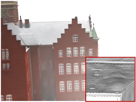
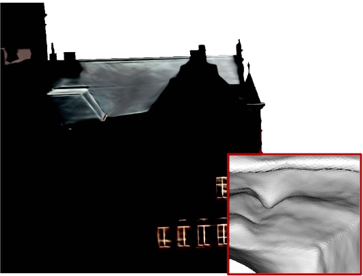
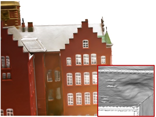
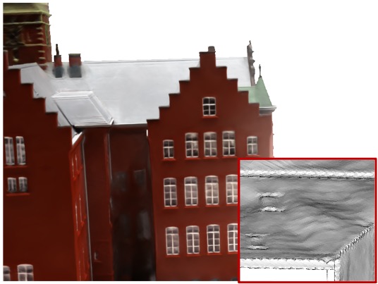
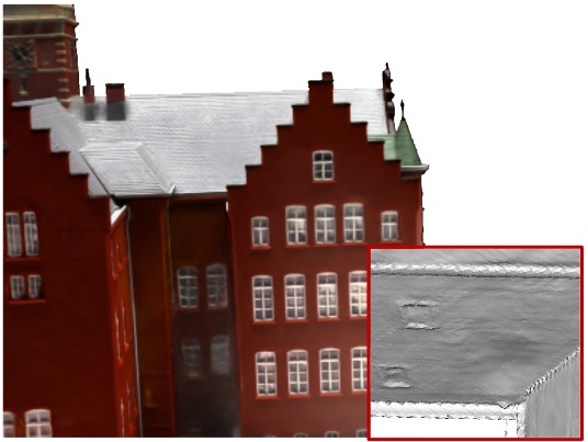
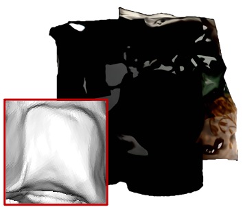
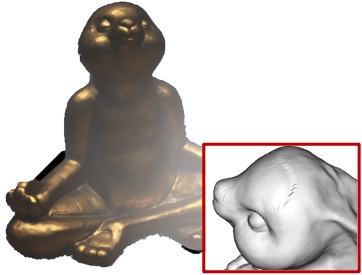
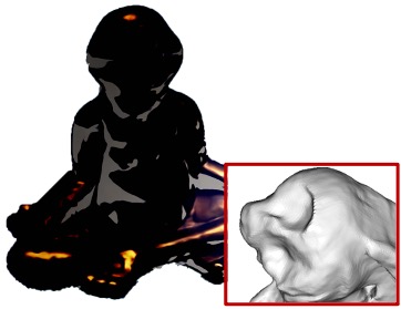
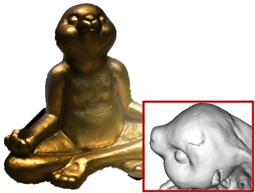
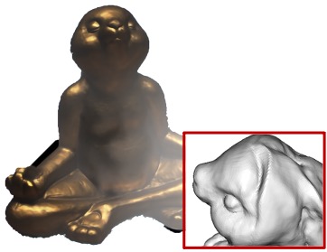
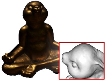
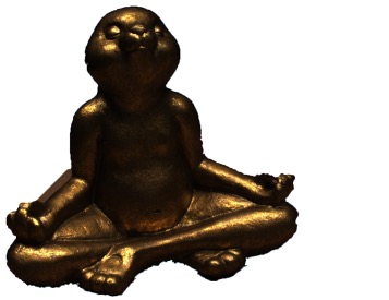
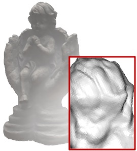
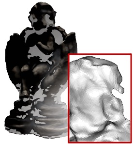
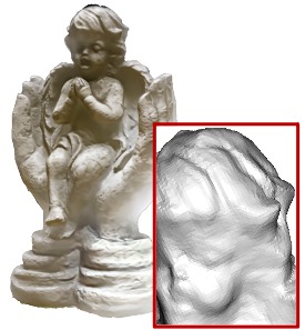
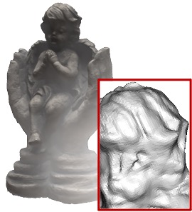
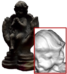
Qualitative Evaluation. We demonstrate some examples of the dehazed results and reconstructed geometry in Fig. 3. Despite having a surface prior, naïvely training HF-NeuS directly from hazy images is equivalent to averaging the scattering-induced geometry-dependent irradiance variance observed across different views and attributing it the surface color. Consequently, the view synthesis is hazy and blurred. For two-stage strategies, the rendered results have color distortion of various degrees, as indicated by the PSNR evaluation in Tab. S.1, since it is difficult to accurately estimate the airlight and coefficient when the presented data does not comply with the specific assumptions or fall in the distribution of the training data. Moreover, our method clearly reconstructs the geometry with more surface details compared to all other baselines that adopt the surface prior formulated in NeuS, since our method can dehaze different views more consistently thanks to the underlying geometry that is optimized jointly.

Quantitative Evaluation. We measure the image quality using peak signal-to-noise ratio (PSNR), structural similarity (SSIM), and perceptual similarity (LPIPS). The geometry quality is measured using Chamfer Distances (CD) using the DTU standard protocol. As shown in Tab. S.1, DehazeNeRF achieves the best results compared to all baselines, with superior performance in PSNR, a metric sensitive to low-frequency color shift. This indicates that while other methods struggle to estimate the true air light and scattering coefficient from either statistical or data priors, our method benefits from jointly optimizing these quantities along with the scene appearance and geometry.

((a)) Without $\mathcal{L}_{\textrm{dcp}}$

((b)) With $\mathcal{L}_{\textrm{dcp}}$

((c)) Ground Truth

((d)) Without $\mathcal{L}_{\textrm{2D}}$

((e)) With $\mathcal{L}_{\textrm{2D}}$

((f)) Ground Truth

Figure 4: Ablation: $\mathcal{L}_{\textrm{dcp}}$ and $\mathcal{L}_{\textrm{2D}}$ lead to more accurate clear-view color photometric details.

Figure 5: Ablation on $\mathcal{L}_{\textrm{2D}}$. We compare the validation results during training with and without $\mathcal{L}_{\textrm{2D}}$: With $\mathcal{L}_{\textrm{2D}}$ the image quality continuously improve.

Method	PSNR ($\uparrow$)	SSIM ($\uparrow$)	LPIPS ($\downarrow$)	Chamfer ($\downarrow$)
NeuS	16.722	0.879	0.087	2.635
COLMAP + NeuS	16.750	0.785	0.225	5.971
ImDehaze[18] + NeuS	17.887	0.899	0.078	2.298
VidDehaze[82] + NeuS	18.324	0.901	0.087	2.349
DehazeNeRF	25.702	0.920	0.052	2.066

Table 1: Quantitative comparison using synthetic data with heterogeneous haze. DehazeNeRF yields better reconstruction both in image quality and geometry accuracy.

4.3 Ablation Study

We conduct ablation studies for the optimization regularizers on 3 scenes and report their average in Tab. 2.

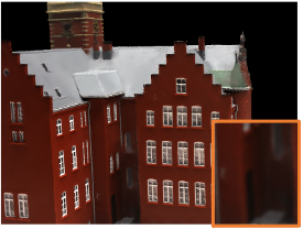
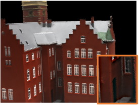
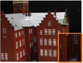
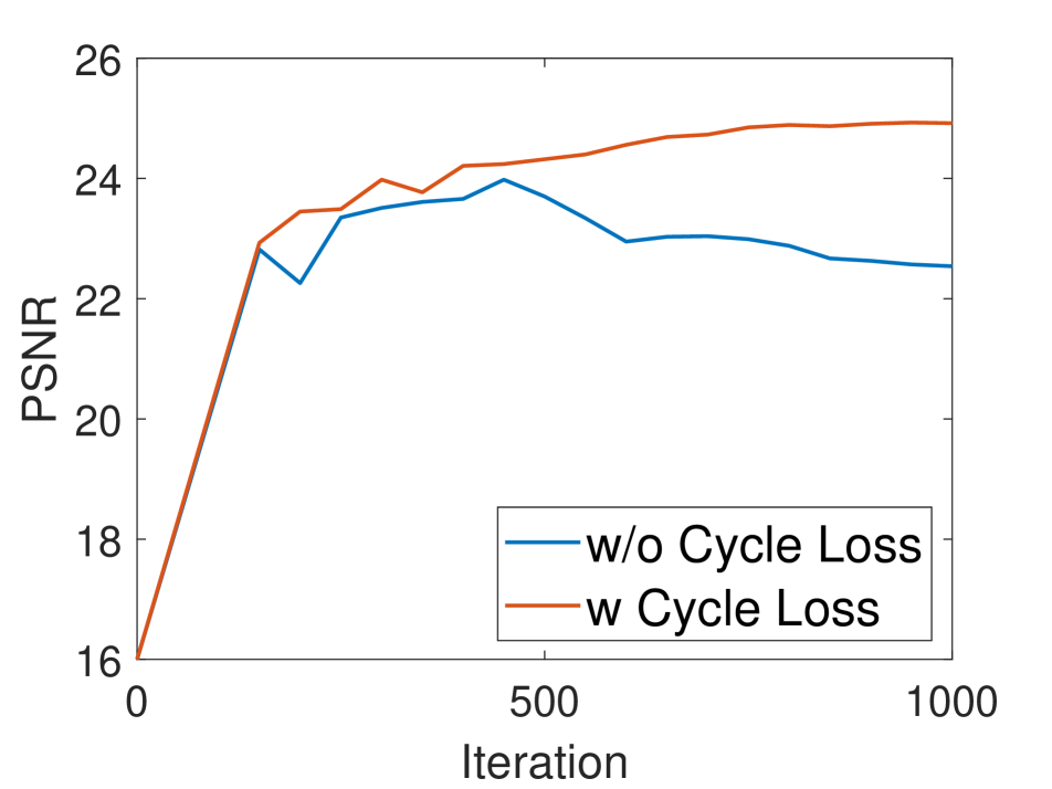
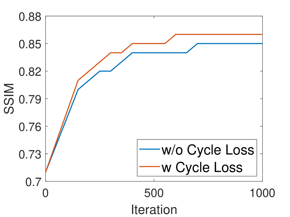
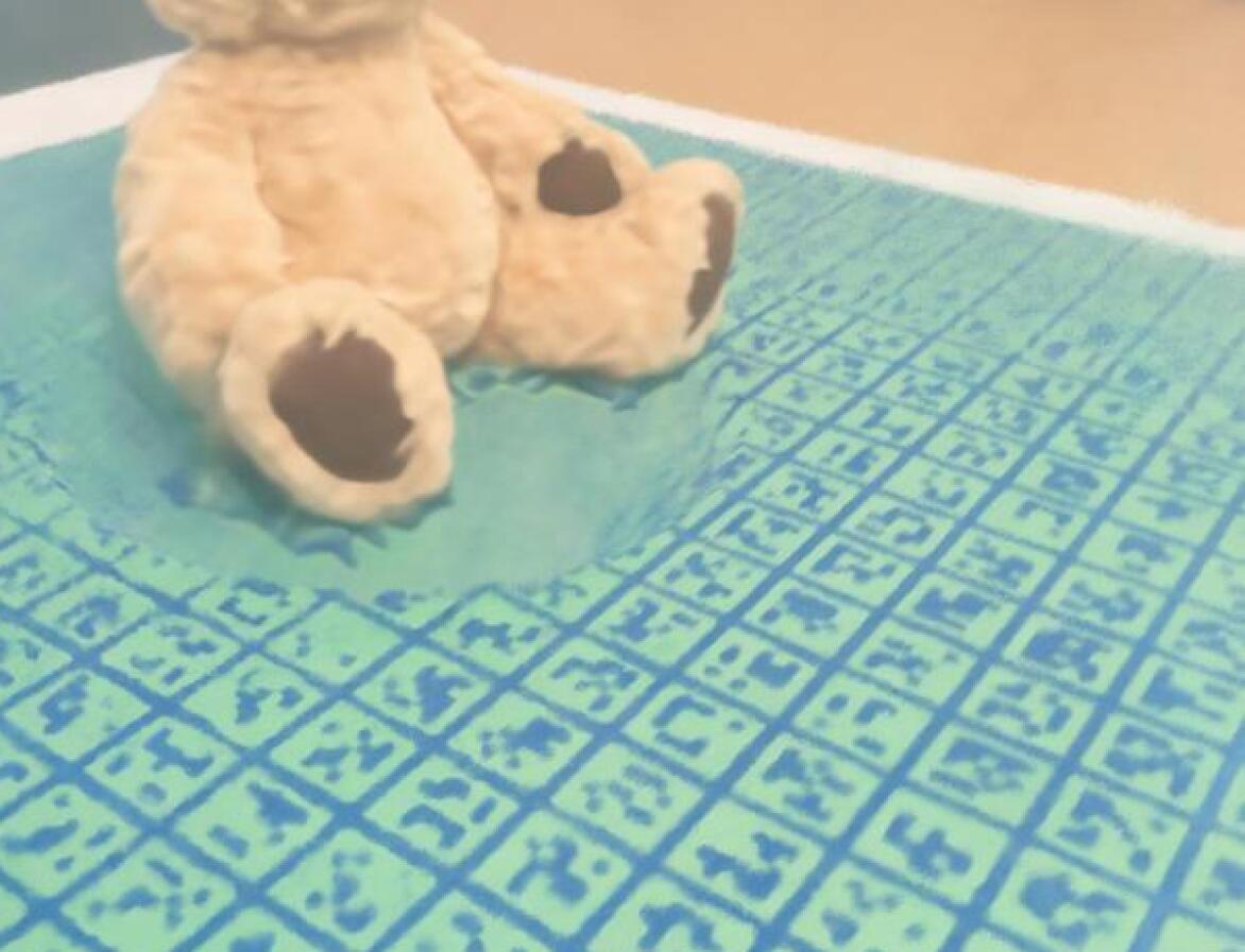
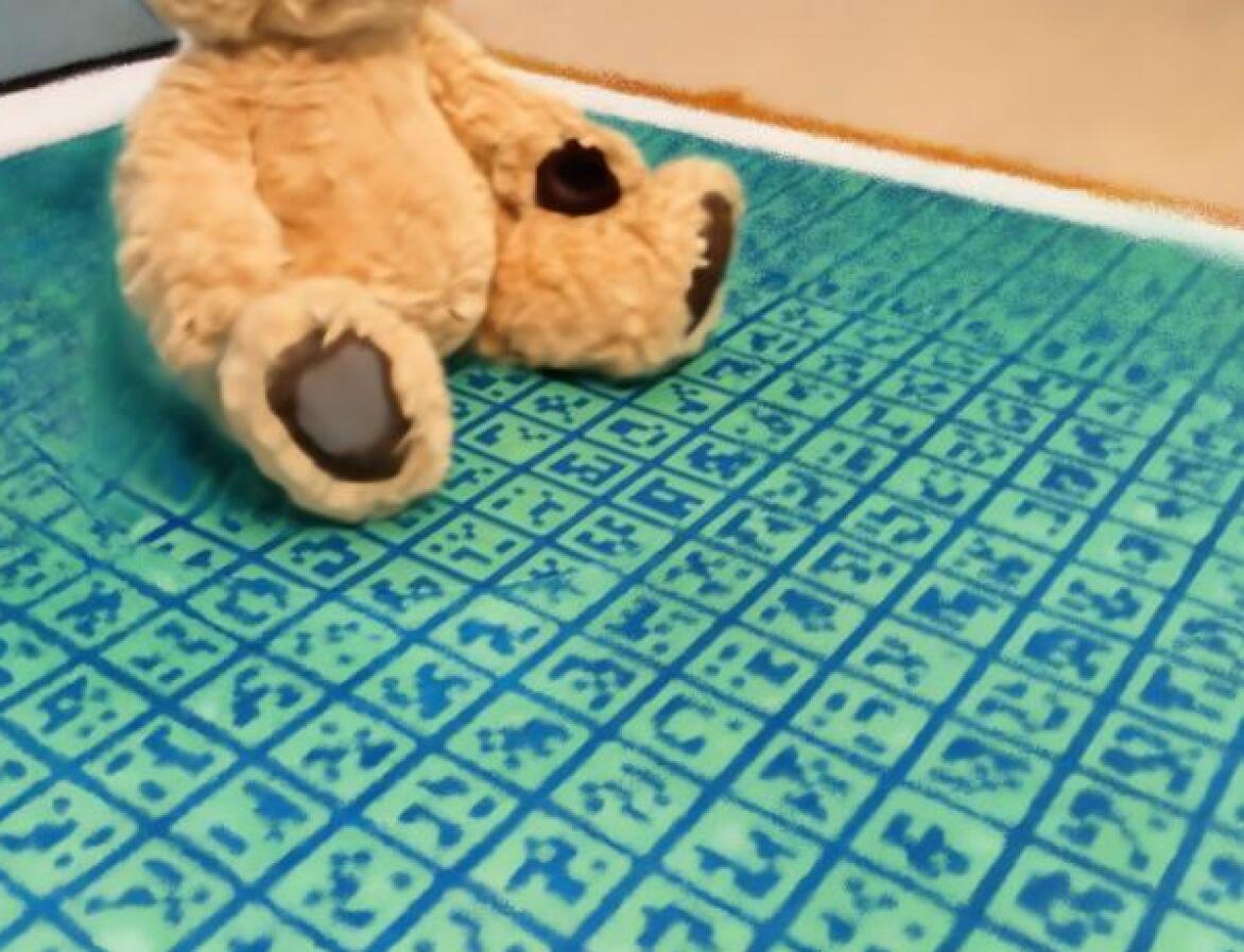
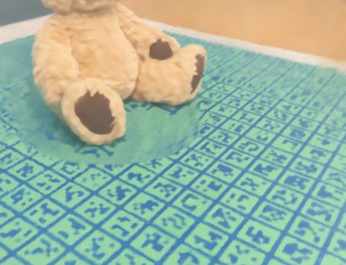
As Tab. 2 shows, both $\mathcal{L}_{\textrm{2D}}$ and $\mathcal{L}_{\textrm{dcp}}$ contribute positively to the image quality and surface reconstruction accuracy. The $\mathcal{L}_{\textrm{dcp}}$ has a prominent effect in reducing global color shift as indicated by the PSNR value. Similarly, from the visual comparison in Figs. 4(a), 4(b) and 4(c), we can observe that by adopting $\mathcal{L}_{\textrm{dcp}}$, the residual haze can be suppressed effectively. Moreover, as shown in Figs. 4(d), LABEL:sub@fig:ablation_cyle_ours and LABEL:sub@fig:ablation_cyle_gt, the results optimized with $\mathcal{L}_{\textrm{2D}}$ show more accurate structure (see orange bounding boxes). In addition, we plot the evolution of validation PSNR and SSIM in Fig. 5. $\mathcal{L}_{\textrm{2D}}$ improves the convergence behavior and yields better validation results.

Method	PSNR ($\uparrow$)	SSIM ($\uparrow$)	LPIPS ($\downarrow$)	Chamfer ($\downarrow$)
w/o $\mathcal{L}_{\textrm{2D}}+\mathcal{L}_{\textrm{dcp}}$	18.21	0.88	0.09	2.47
w $\mathcal{L}_{\textrm{2D}}$	18.53	0.89	0.09	2.44
w $\mathcal{L}_{\textrm{dcp}}$	24.02	0.90	0.06	2.44
DehazeNeRF	25.23	0.91	0.05	2.41

Table 2: Ablations on regularization. Each of the proposed two regularizations can individually improve the image and geometry reconstruction, and the best quality is achieved with both. The results are averaged from 10 test scenes from the DTU dataset.

NeuS	COLMAP + NeuS	ImDehaze + NeuS	VidDehaze + NeuS	DehazeNeRF	Ground Truth

Figure 6: Qualitative comparison on captured data. Our method recovers the haze-free scenes with more image details and colors closer to the ground truth.

Method	PSNR ($\uparrow$)	SSIM ($\uparrow$)	LPIPS ($\downarrow$)
NeuS	12.60	0.48	0.38
COLMAP + NeuS	9.27	0.38	0.47
ImDehaze + NeuS	13.35	0.49	0.36
VidDehaze + NeuS	14.56	0.50	0.34
DehazeNeRF	17.47	0.68	0.16

Table 3: Quantitative evaluation on experimentally captured data averaged over 3 scenes. Our method outperforms other methods by a large margin.

5 Experimentally Captured Results

5.1 Data Collection

We captured three indoor hazy scenes using two professional haze machines and an iPhone 12 Pro. The scenes contain 38, 82, and 68 hazy images and 79, 47, and 47 clear images for testing respectively. To ensure temporal consistency (dynamic haze is out of scope for this paper), we capture the data after the haze has settled and appears steady. After the capturing, we merge hazy images and clear images under the same scene and adopt COLMAP to register camera positions, which yields a consistent registration for the hazy and clear view for ease of evaluation. We scale and translate the object such that it lies inside the unit sphere and roughly at the center of the world coordinates. More details on the data capture are described in the supplement.

5.2 Implementation details.

Several changes are applied to the model to facilitate the optimization for captured data. First, we remove the mask loss ( Eq. 21). Second, similar to NeuS [71], the region outside uses the parameterization of NeRF++[81], for which we also applied the haze attenuation following Eqs. 8, 3.3 and 9.

5.3 Comparison

For evaluation, we adopt the same baselines described in Sec. 4.2. The 2D photometric quality is evaluated using the same metrics, and geometry reconstruction quality is omitted due to the lack of ground truth.

Quantitative Evaluation.

The results are reported in Tab. 3. One can observe that our method outperforms other baselines in all metrics, demonstrating the robustness of the proposed method in the real-world scenario.

Qualitative Evaluation.

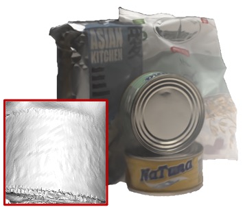
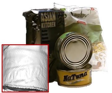
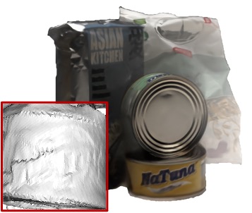
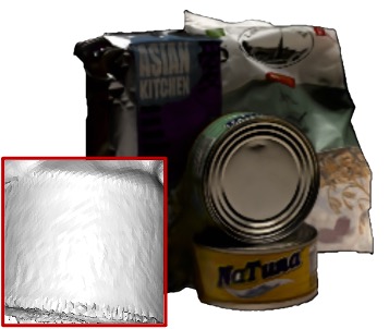
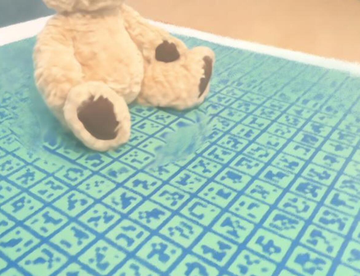
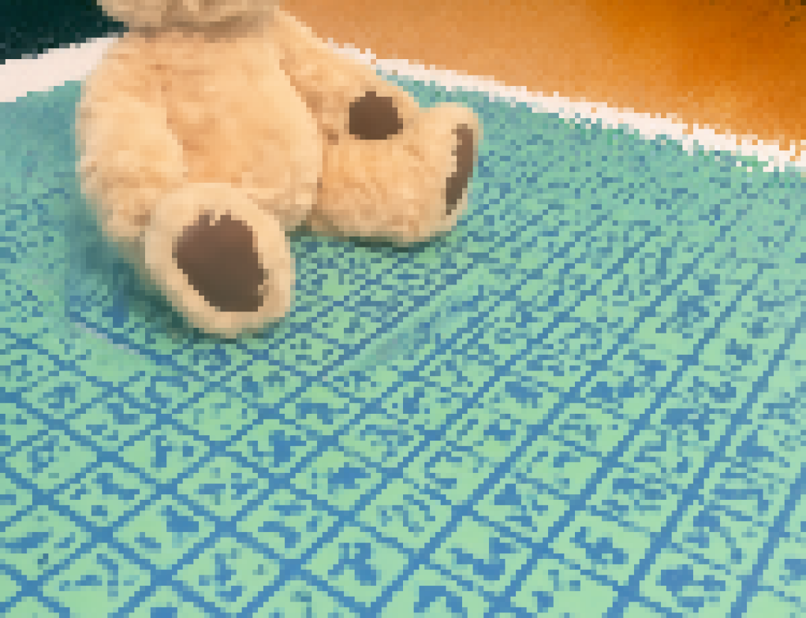
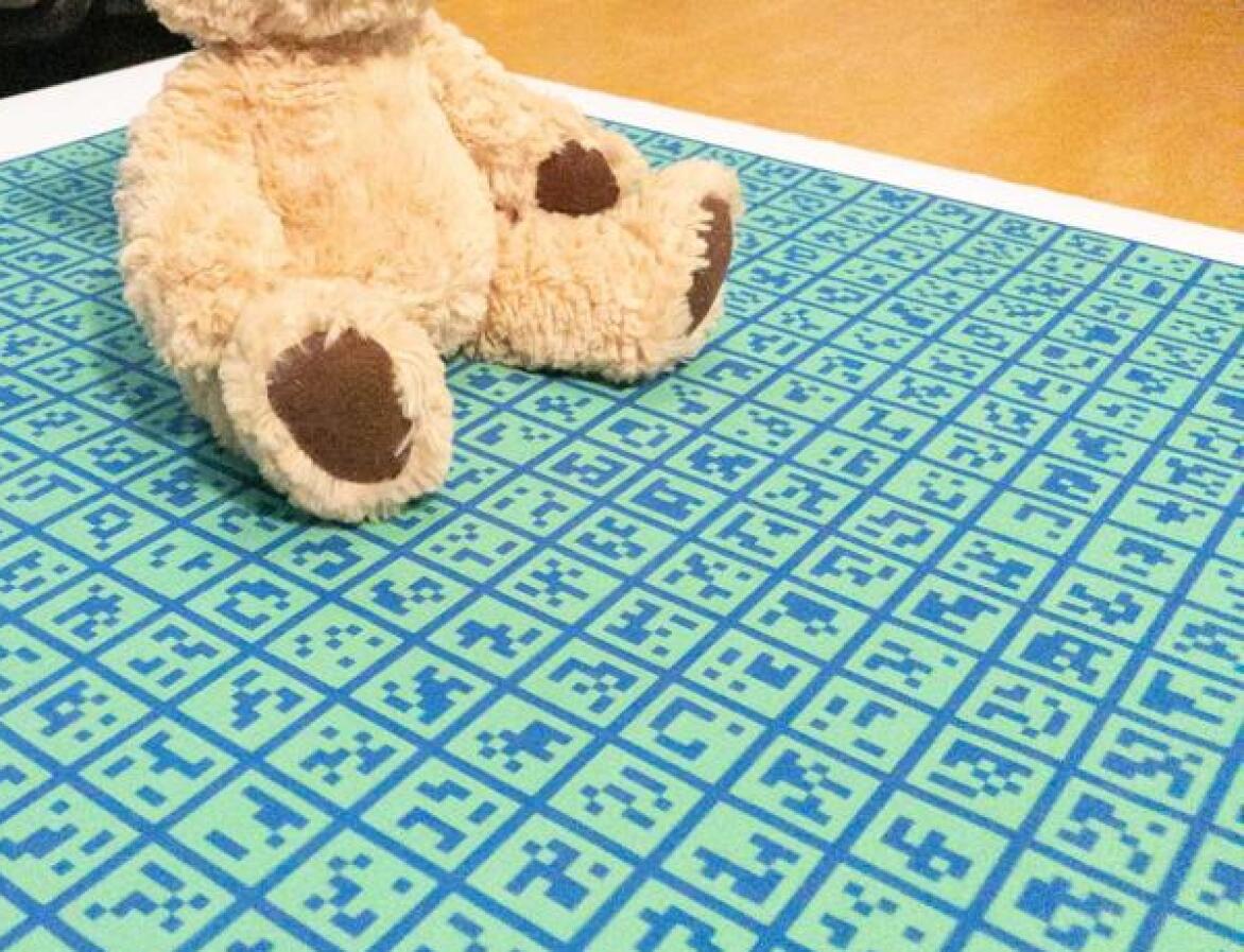
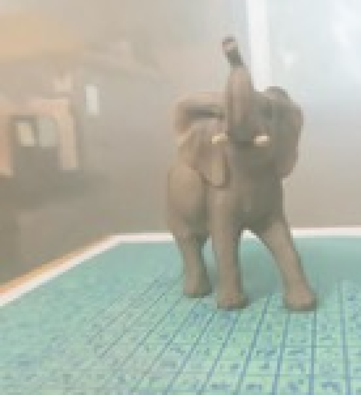
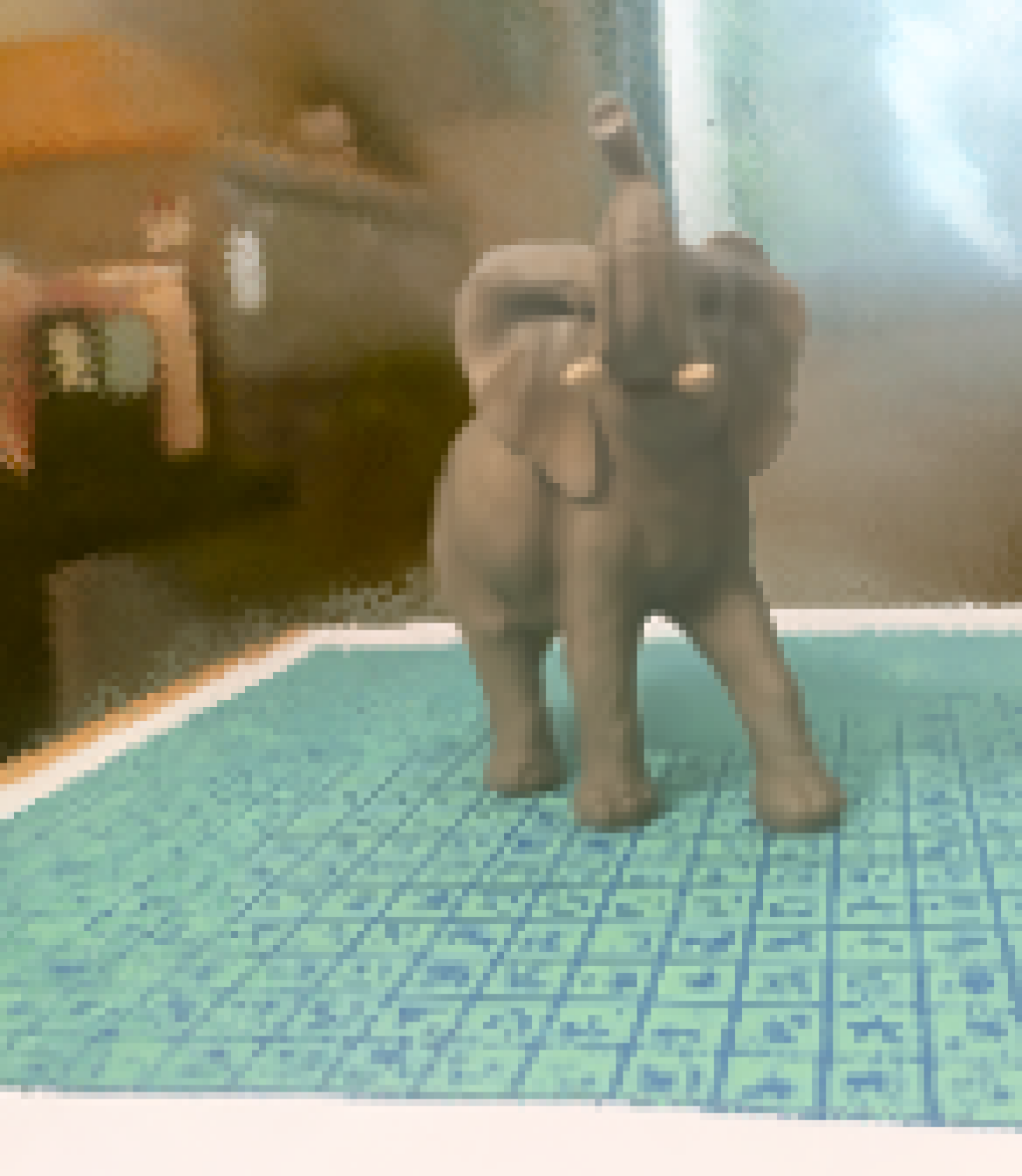
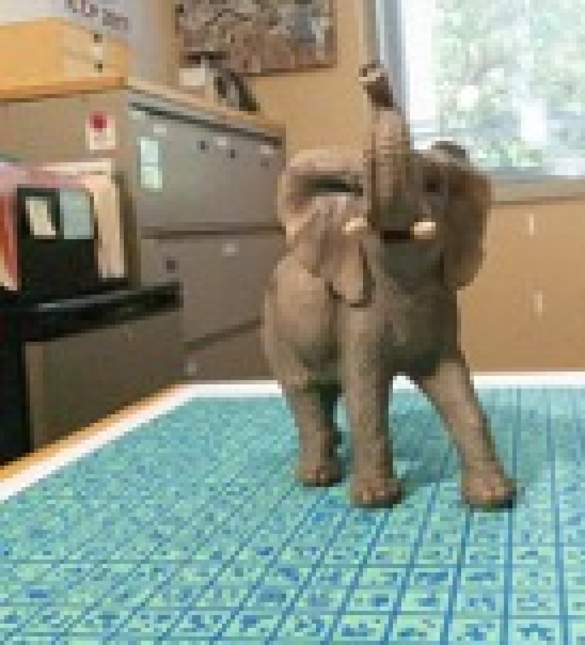
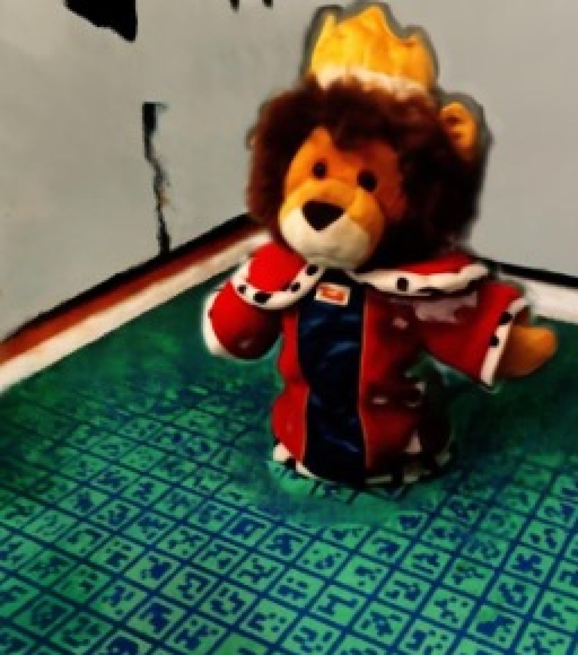
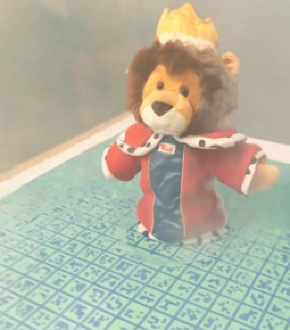
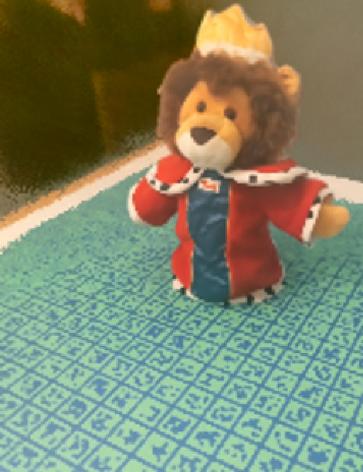
As shown in Fig. 6, vanilla NeuS includes haze in the synthesized views. On the other hand, adopting 2D image dehazing or video dehazing methods as pre-processing also cannot generate desired clear results since these learning-based models have limited generalization ability in real-world data. Although using COLMAP as pre-processing can suppress residual haze, the dehazed results tend to have the color distortion problem and the limited structure (see the background at the $3^{rd}$ column of Fig. 6). Our method achieves significantly better visual quality compared to other baselines.

6 Discussion

In this paper, we address challenges to apply NeRFs in hazy scenes. Our method jointly learns the 3D structure and the plausible clear-view appearance of the scene, as well as the haze properties (airlight and scattering coefficient) from hazy observations. Our key technical contributions are: 1. incorporating the scattering phenomena in NeRF’s rendering equation; 2. deploying physically inspired inductive biases and haze-specific regularizers to disambiguate haze and clear-view components. The proposed techniques take a significant step towards adopting NeRF-related approaches in real-life scenarios where adverse weather conditions are detrimental to 3D reconstruction.

Relation to the Koschmieder Law.

Koschmieder model is a 2D image formation model that describes the relationship between the clear-view and the hazy images. Assuming homogeneous scattering, our formulation can be simplified to Koschmieder’s model, which reduces to supervising with Eq. S.7 and $\mathcal{L}_{\textrm{dcp}}$. Our $\mathcal{L}_{\textrm{2D}}$ exploits this relation to improve the convergence as shown in Sec. 4.3. In Tab. 4, we examine this relation by comparing this simplified method (denoted as Koschm) with a variant of DehazeNeRF that uses a learnable scalar instead of the proposed MLP to model the scattering coefficient (denoted as Scalar). For both synthetic and real data, the Scalar and Koschm solutions are comparable, which validates the relation to Koschmieder law; our full model shows a considerable advantage in both scenarios thanks to its more general formulation.

Method	Synthetic Data (Scene24)				Real Data (“Elephant” Scene)
	PSNR	SSIM	LPIPS	Chamfer	PSNR	SSIM	LPIPS
Koschm	18.62	0.79	0.13	1.44	16.84	0.69	0.18
Scalar	18.50	0.79	0.13	1.46	16.80	0.69	0.18
DehazeNeRF	22.78	0.82	0.09	1.22	17.87	0.73	0.15

Table 4: Relation to the 2D Koschmieder Law. When using a scalar to model the scattering coefficient (Scalar), our method can simplify to supervising with the 2D Koschmieder law (Koschm). Our full model using an MLP to model the spatially varying scattering coefficient has a clear advantage for heterogeneous haze.

Limitations and future work.

While we have demonstrated the effectiveness of our method to capture data, certain scenarios are not addressed in the scope of this paper and are research directions for future work. These include severe haze scenes, where camera registration fails due to the lack of discriminative image features, and dynamic haze, where the haze distribution change not only spatially but also temporally. Nonetheless, we believe that our method is an important step towards anticipated application scenarios, such as autonomous driving or underwater imaging. The principle of incorporating physics into the neural rendering is also applicable to other ill-posed low-level vision tasks, such as image denoising, image brightening, and super-resolution.

Supplemental Materials

Data	Method	PSNR $\uparrow$	SSIM $\uparrow$	LPIPS $\downarrow$	Chamfer $\downarrow$
Scan 24	NeuS	13.93	0.72	0.19	1.51
	COLMAP+NeuS	11.82	0.41	0.54	6.22
	ImDehaze[18]+NeuS	16.83	0.80	0.18	1.60
	VidDehaze[82]+NeuS	16.73	0.77	0.19	1.59
	DehazeNeRF	22.78	0.82	0.09	1.22
Scan 37	NeuS	20.64	0.88	0.06	1.44
	COLMAP+NeuS	13.34	0.75	0.23	3.04
	ImDehaze[18]+NeuS	21.55	0.90	0.06	1.90
	VidDehaze[82]+NeuS	20.90	0.88	0.08	2.16
	DehazeNeRF	21.61	0.90	0.06	1.43
Scan 83	NeuS	20.25	0.94	0.05	7.03
	COLMAP+NeuS	17.23	0.92	0.08	7.10
	ImDehaze[18]+NeuS	22.89	0.94	0.05	7.01
	VidDehaze[82]+NeuS	21.12	0.95	0.05	7.03
	DehazeNeRF	28.46	0.95	0.03	6.91
Scan 97	NeuS	17.32	0.91	0.07	2.08
	COLMAP+NeuS	16.93	0.77	0.25	2.96
	ImDehaze[18]+NeuS	18.18	0.93	0.07	2.02
	VidDehaze[82]+NeuS	18.61	0.93	0.07	2.05
	DehazeNeRF	24.41	0.92	0.05	1.89
Scan 105	NeuS	18.98	0.93	0.07	2.65
	COLMAP+NeuS	15.65	0.77	0.33	3.78
	ImDehaze[18]+NeuS	18.84	0.94	0.06	2.64
	VidDehaze[82]+NeuS	17.74	0.92	0.09	2.95
	DehazeNeRF	26.18	0.95	0.04	2.65
Scan 106	NeuS	14.57	0.84	0.11	4.24
	COLMAP+NeuS	17.03	0.78	0.22	2.29
	ImDehaze[18]+NeuS	15.45	0.86	0.09	1.34
	VidDehaze[82]+NeuS	17.20	0.89	0.11	1.67
	DehazeNeRF	28.41	0.92	0.07	1.23
Scan 110	NeuS	15.21	0.86	0.13	1.90
	COLMAP+NeuS	19.01	0.84	0.20	2.88
	ImDehaze[18]+NeuS	17.53	0.89	0.10	2.30
	VidDehaze[82]+NeuS	15.69	0.86	0.13	2.11
	DehazeNeRF	23.28	0.93	0.06	1.76
Scan 114	NeuS	16.88	0.90	0.07	0.86
	COLMAP+NeuS	15.60	0.82	0.17	1.19
	ImDehaze[18]+NeuS	17.39	0.92	0.06	0.80
	VidDehaze[82]+NeuS	19.96	0.93	0.06	0.87
	DehazeNeRF	22.73	0.91	0.06	0.84
Scan 118	NeuS	14.47	0.86	0.09	2.64
	COLMAP+NeuS	18.28	0.82	0.17	1.90
	ImDehaze[18]+NeuS	15.14	0.88	0.07	1.66
	VidDehaze[82]+NeuS	17.57	0.91	0.08	1.53
	DehazeNeRF	28.28	0.92	0.05	1.25
Scan 122	NeuS	15.35	0.90	0.07	1.23
	COLMAP+NeuS	19.83	0.85	0.17	1.57
	ImDehaze[18]+NeuS	15.95	0.92	0.06	1.35
	VidDehaze[82]+NeuS	18.05	0.92	0.08	1.22
	DehazeNeRF	28.55	0.94	0.06	0.99
Average	NeuS	16.72	0.88	0.09	2.64
	COLMAP+NeuS	16.75	0.79	0.23	5.97
	ImDehaze[18]+NeuS	17.89	0.90	0.08	2.30
	VidDehaze[82]+NeuS	18.32	0.90	0.09	2.35
	DehazeNeRF	25.70	0.92	0.05	2.07

Table S.1: Quantitative evaluation for synthetic haze dataset.

Appendix A Data generation

A.1 Synthetic Data

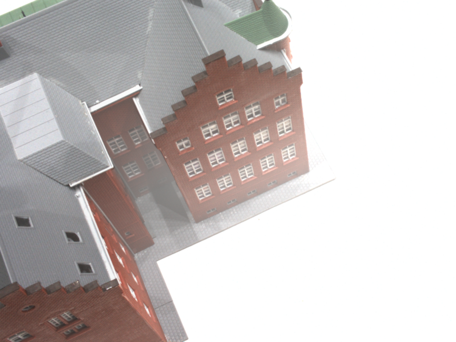
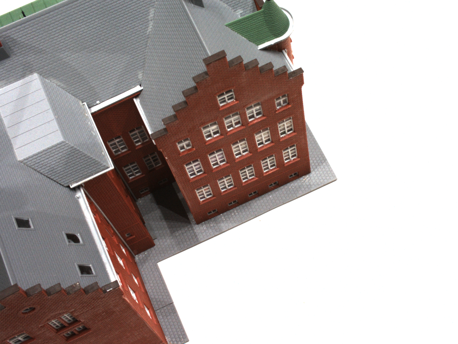
An example of our synthesized results are shown in Fig. S.1. The scattering coefficient is modeled using the sum of 4 scaled Gaussian blobs located inside the spatial bounding box with a standard deviation uniformly sampled from 1.0 to 3.0; the 3-D atmospheric light is sampled from a uniform distribution in the range $[0.7,0.9]$.

Figure S.1: An example of the synthetic data. Right: original input image. Left: synthetic hazy input with heterogeneous scattering.

A.2 Real Data Collection

We use two professional haze machines to generate a dense vapor. These haze generators adopt cast or platen-type aluminum heat exchangers, which make evaporation of the water-based haze liquid. We capture our scenes in a hermetic chamber. First, we captured clear reference images from different view directions. Then, we employed 2 minutes for both haze machines and waited for another 2 minutes until the haze was temporally stable. We then captured hazy images from different viewpoints. An iPhone 12 was used as our camera. The camera’s settings including exposure, iso, and focal length were the same for all captures.

After the capturing, we merge hazy images and clear images under the same scene and run COLMAP [59, 60] to register camera positions.

Appendix B Evaluation

Quantitative Evaluation on Synthetic Dataset

We present the complete quantitative results on DTU dataset [25] in Tab. S.1. One can see that the proposed DehazeNeRF outperforms other baselines in most of the scenes in terms of image quality and geometric reconstruction.

Surface Prior	PSNR$\uparrow$	SSIM$\uparrow$	LPIPS$\downarrow$	Chamfer$\downarrow$
None	21.331	0.901	0.071	4.013
via NeuS	26.039	0.921	0.056	2.863

Table S.2: The effect of NeuS surface prior evaluated on 5 test scenes.

Additional Ablation

Here, we present an additional ablation to demonstrate the effect of using the NeuS surface prior. To this end, we replace the NeuS backbone with a NeRF [46] backbone and compare the image quality and geometry reconstruction performance. As shown in Tab. S.2, by adopting a surface prior, implemented via the surface-based parameterization of the volume density NeuS, the model can converge to a better solution in terms of haze-surface disambiguation leading to significantly better image and geometry reconstruction quality.

Appendix C Implementation Detail

Network architecture

We adopt a similar network architecture as HF-NeuS [73]. It contains two MLPs to encode surface SDF and surface color respectively. The SDF MLP consists of 8 hidden layers with hidden size of 256. A skip connection is applied from the input to the fourth hidden layer. The color MLP contains 4 hidden layers with size of 256. It takes the spatial location p, the view direction d, the normal vector of SDF, and a 256-dimensional feature vector from the SDF MLP. Positional encoding is applied to spatial location and view direction with 6 and 4 frequencies, respectively.

For the spatially variant scattering coefficient, we adopt band-limited coordinate networks [34] using 3 hidden layers, where each layer has 32 channels and the frequency parameter set to 10.

Training and inference details

We train the proposed DehazeNeRF by using the Adam optimizer [30]. We set the learning rate linearly from 0 to $5\times 10^{-4}$ by warmed up strategy in the first 5k iterations. Then, we reduce the learning rate by the cosine decay schedule to the minimum learning rate $2.5\times 10^{-5}$. We train our model for 24 hours (for the ‘w/ mask’ setting) and 26 hours (for the ‘w/o mask’ setting) on a single Nvidia Tesla V100 GPU with batch size 512, respectively. For the first 300k iterations, we set the scattering coefficients and atmospheric light as zero and train the model based on the vanilla HF-NeuS. In this stage, we disable the Koschmieder Consistency and dark channel losses. After 300k iterations, the scattering coefficients and atmospheric light are introduced and optimized with the Koschmieder Consistency and dark channel losses. We train our network for 800k and 50k iterations for synthetic and captured data, respectively. The scale factors $\lambda$, $\alpha$, and $\beta$ in the loss function are set to 0.1, 5000, and 0.01 for synthetic data and 0.1, 1.0, and 0.01 for the captured dataset, respectively. The scale factor of mask loss is set to 0.1. For the inference stage, it takes 200 seconds to render an image in resolution of $1600\times 1200$.

Appendix D Deriving DehazeNeRF

D.1 Radiative Transfer Equation

Radiative transfer equation (RTE) [6, 65] describes the behaviour of light in a medium that absorbs, scatters and emits radiation. Assuming, a ray $\mathbf{r}\left(t\right)=\mathbf{o}+t\mathbf{d}$ hits a surface point at $\mathbf{r}\left(t_{0}\right)$, the incident radiance at the near image plane $t_{n}$ can be divided into three parts [53]:

$$\begin{split}C(\mathbf{r},\mathbf{d})=&\underbrace{\int_{t_{n}}^{t_{0}}\epsilon\left(\mathbf{r}\left(t\right),\mathbf{d}\right)T_{\sigma_{t}}\left(t\right)dt}_{\textrm{emission}}\\ &+\underbrace{\int_{t_{n}}^{t_{0}}c_{\textrm{s}}\left(\mathbf{r}\left(t\right),\mathbf{d}\right)\sigma_{s}\left(\mathbf{r}\left(t\right)\right)T_{\sigma_{t}}\left(t\right)dt}_{\textrm{in-scattering}}\\ &+\underbrace{C_{e}\left(\mathbf{r}\left(t_{0}\right),\mathbf{d}\right)T_{\sigma_{t}}\left(t_{0}\right)}_{\textrm{surface reflection}},\end{split}$$ (S.1)

where $\epsilon$ is the emission, $C_{e}$ is the outgoing radiance at the surface intersection, $c_{\textrm{s}}\left(\mathbf{r}\left(t\right),\mathbf{d}\right)$ is the in-scattered light and $\sigma_{s}$ is the scattering coefficient. In particular the transmittance here is computed from the attenuation coefficient $\sigma_{t}$, i.e., $T_{\sigma_{t}}\left(t\right)=\exp\left(-\int_{t_{n}}^{t}\sigma_{t}(t^{\prime})dt^{\prime}\right)$, where $\sigma_{t}=\sigma_{a}+\sigma_{s}$ including the absorption and out-scattering effect.

Based on this equation, we then connect it to the neural radiance field (NeRF) and hazy image formation model.

D.2 From RTE to NeRF

For the volume rendering equation adopted in NeRF, there are two assumptions: (i) no scattering and (ii) only absorption and emission are considered. The volume rendering equation can be derived by the RTE equation by dropping the in-scattering term and combining the surface reflection term into the emission term. It can be presented as: [42, 71, 75]

$$\begin{split}C(\mathbf{r},\mathbf{d})=&\underbrace{\int_{t_{n}}^{t_{0}}\epsilon\left(\mathbf{r}\left(t\right),\mathbf{d}\right)T_{\sigma_{a}}\left(t\right)dt}_{\textrm{emission}}\\ &+\underbrace{C_{e}\left(\mathbf{r}\left(t_{0}\right),\mathbf{d}\right)T_{\sigma_{a}}\left(t_{0}\right)}_{\textrm{surface reflection}}.\end{split}$$ (S.2)

Since NeRF treats each point as an emission point, the radiance of the surface can be considered as emission at $t_{0}$. Thus, the surface reflection in Eq. S.2 becomes

Therefore Eq. S.2 can be written as:

$$\begin{split}C(\mathbf{r},\mathbf{d})&=\int_{t_{n}}^{t_{0}}\epsilon_{\textrm{combined}}\left(\mathbf{r}\left(t\right),\mathbf{d}\right)T_{\sigma_{a}}\left(t\right)dt,\end{split}$$ (S.4)

where $\epsilon_{\textrm{combined}}=\epsilon\left(\mathbf{r}\left(t\right),\mathbf{d}\right)+\epsilon_{o}\left(\mathbf{r}\left(t_{0}\right),\mathbf{d}\right)\delta(t-t_{0})$.

By further setting $\epsilon_{\textrm{combined}}\left(\mathbf{r}\left(t\right),\mathbf{d}\right)=c(\mathbf{r}(t),\mathbf{d})\sigma(\mathbf{r}(t))$ and $\sigma_{a}=\sigma$, we can see Eq. S.4 is the same as famous NeRF rendering equation below:

$$\begin{split}{C}(\mathbf{r},\mathbf{d})=\int_{t_{n}}^{t_{f}}c(\mathbf{r}(t),\mathbf{d})\sigma(\mathbf{r}(t))T(t)\ dt.\end{split}$$ (S.5)

In practice, absorption coefficient $\sigma_{a}(\mathbf{r}(t))$ describes the probability of a photon being absorbed at position $\mathbf{r}\left(t\right)$, while $\sigma(\mathbf{r}(t))$ (called volume density in NeRF) illustrates the probability of a ray terminating at location $\mathbf{r}\left(t\right)$. That is, $\sigma_{a}$ is the same meaning as $\sigma$ physically since NeRF only considers the absorption. Moreover, generally, we can assume that when the ray hits the object, the attenuation term (accumulative transmittance) may become zero. That is, $T(t)\cong 0$ when $t>t_{0}$. Thus, the integral from $t_{n}$ to $t_{f}$ is approximately equal to that from $t_{n}$ to $t_{0}$.

D.3 From RTE to Koschmieder Model

For the conventional haze formation model, there are three assumptions[44, 47]: (i) no emission, (ii) only consider single scattering, and (iii) only consider scattering since absorption in atmospheric particles is relatively small. Therefore, Eq. S.1 simplifies to

$$C(\mathbf{r},\mathbf{d})= \underbrace{\int_{t_{n}}^{t_{0}}c_{\textrm{s}}\left(\mathbf{r}\left(t\right),\mathbf{d}\right)\sigma_{s}\left(\mathbf{r}\left(t\right)\right)T_{\sigma_{s}}\left(t\right)dt}_{\textrm{in-scattering}}$$

$$+\underbrace{C_{e}\left(\mathbf{r}\left(t_{0}\right),\mathbf{d}\right)T_{\sigma_{s}}\left(t_{0}\right)}_{\textrm{surface reflection}}.$$ (S.6)

Assuming the scattering coefficient and atmospheric light are isotropic and homogeneous, i.e., $\sigma_{s}\left(\mathbf{r}\left(t\right)\right)\equiv\bar{\sigma}_{s}$ and $c_{s}\left(\mathbf{r}\left(t\right),\mathbf{d}\right)\equiv\bar{c}_{s}$, setting $t_{n}=0$ and $C_{e}\left(\mathbf{r}\left(t_{0}\right),\mathbf{d}\right)=C_{\textrm{clear}}$, we can rewrite Eq. S.6 to the Koschmieder model [24], namely

D.4 3D Haze Formation in DehazeNeRF

In this part, we bring Eq. S.6 to a similar form as NeRF so that we can learn the geometry and color through samples in the 3D space.

First, we bring back volume density $\sigma$, i.e., replace $\sigma_{s}$ with $\sigma_{t}=\sigma_{s}+\sigma$:

$$\begin{split}C(\mathbf{r},\mathbf{d})=\int_{t_{n}}^{t_{0}}c_{\textrm{s}}\left(\mathbf{r}\left(t\right),\mathbf{d}\right)\sigma_{s}\left(\mathbf{r}\left(t\right)\right)T_{\sigma_{t}}\left(t\right)dt\\ +C_{e}\left(\mathbf{r}\left(t_{0}\right),\mathbf{d}\right)T_{\sigma_{t}}\left(t_{0}\right),\end{split}$$ (S.8)

which corresponds to Eq. (3) in the main paper. Using the same trick in Eq. S.3, we can combine the surface reflection term into the integral and obtain the rendering equation used in DehazeNeRF (Eq. (4) in the main paper):

$$C(\mathbf{r},\mathbf{d})= \int_{t_{n}}^{t_{0}}c_{\textrm{s}}\left(\mathbf{r}\left(t\right),\mathbf{d}\right)\sigma_{s}\left(\mathbf{r}\left(t\right)\right)T_{\sigma_{t}}\left(t\right)dt$$

$$+\int_{t_{n}}^{t_{0}}\underbrace{\epsilon_{\textrm{surface}}\left(\mathbf{r}\left(t_{0}\right),\mathbf{d}\right)}_{\epsilon_{o}\left(\mathbf{r}\left(t_{0}\right),\mathbf{d}\right)\delta(t-t_{0})}T_{\sigma_{t}}\left(t\right)dt$$

$$= {\int_{t_{n}}^{t_{0}}c_{\textrm{s}}\left(\mathbf{r}\left(t\right),\mathbf{d}\right)\sigma_{s}\left(\mathbf{r}\left(t\right)\right)T_{\sigma_{t}}\left(t\right)dt}$$

$$+{\int_{t_{n}}^{t_{0}}\underbrace{c\left(\mathbf{r}\left(t\right),\mathbf{d}\right)\sigma\left(\mathbf{r}\left(t\right)\right)}_{\epsilon_{\textrm{surface}}\left(\mathbf{r}\left(t_{0}\right),\mathbf{d}\right)}T_{\sigma_{t}}\left(t\right)dt}.$$ (S.9)

The first term (denoted as $C_{\text{haze}}$) captures the radiance caused by haze scattering. The second term (denoted as $C_{\textrm{surface}}$) is equivalent to NeRF for a scene with only solid surfaces.

References

- [1] Codruta O Ancuti, Cosmin Ancuti, Radu Timofte, Luc Van Gool, Lei Zhang, and Ming-Hsuan Yang. Ntire 2019 image dehazing challenge report. In Proceedings of the IEEE/CVF Conference on Computer Vision and Pattern Recognition Workshops, pages 0–0, 2019.
- [2] Dana Berman, Shai Avidan, et al. Non-local image dehazing. In Proceedings of the IEEE conference on computer vision and pattern recognition, pages 1674–1682, 2016.
- [3] Jacopo Bertolotti, Elbert G Van Putten, Christian Blum, Ad Lagendijk, Willem L Vos, and Allard P Mosk. Non-invasive imaging through opaque scattering layers. Nature, 2012.
- [4] David A Boas, Dana H Brooks, Eric L Miller, Charles A DiMarzio, Misha Kilmer, Richard J Gaudette, and Quan Zhang. Imaging the body with diffuse optical tomography. IEEE signal processing magazine, 18(6):57–75, 2001.
- [5] Trung Minh Bui and Wonha Kim. Single image dehazing using color ellipsoid prior. IEEE Transactions on Image Processing, 27(2):999–1009, 2017.
- [6] Subrahmanyan Chandrasekhar. Radiative transfer. Courier Corporation, 2013.
- [7] Wei-Ting Chen, Jian-Jiun Ding, and Sy-Yen Kuo. Pms-net: Robust haze removal based on patch map for single images. In Proceedings of the IEEE/CVF Conference on Computer Vision and Pattern Recognition, pages 11681–11689, 2019.
- [8] Xingyu Chen, Qi Zhang, Xiaoyu Li, Yue Chen, Ying Feng, Xuan Wang, and Jue Wang. Hallucinated neural radiance fields in the wild. In Proceedings of the IEEE/CVF Conference on Computer Vision and Pattern Recognition, pages 12943–12952, 2022.
- [9] Won Young Chung, Sun Young Kim, and Chang Ho Kang. Image dehazing using lidar generated grayscale depth prior. Sensors, 22(3):1199, 2022.
- [10] Hang Dong, Jinshan Pan, Lei Xiang, Zhe Hu, Xinyi Zhang, Fei Wang, and Ming-Hsuan Yang. Multi-scale boosted dehazing network with dense feature fusion. In Proceedings of the IEEE/CVF conference on computer vision and pattern recognition, pages 2157–2167, 2020.
- [11] C Dunsby and PMW French. Techniques for depth-resolved imaging through turbid media including coherence-gated imaging. Journal of Physics D: Applied Physics, 36(14):R207, 2003.
- [12] Daniele Faccio, Andreas Velten, and Gordon Wetzstein. Non-line-of-sight imaging. Nature Reviews Physics, 2(6):318–327, 2020.
- [13] Raanan Fattal. Dehazing using color-lines. ACM transactions on graphics (TOG), 34(1):1–14, 2014.
- [14] Yuki Fujimura, Motoharu Sonogashira, and Masaaki Iiyama. Dehazing cost volume for deep multi-view stereo in scattering media. In Proceedings of the Asian Conference on Computer Vision, 2020.
- [15] Adam Gibson and Hamid Dehghani. Diffuse optical imaging. Philosophical Transactions of the Royal Society A: Mathematical, Physical and Engineering Sciences, 367(1900):3055–3072, 2009.
- [16] Amos Gropp, Lior Yariv, Niv Haim, Matan Atzmon, and Yaron Lipman. Implicit geometric regularization for learning shapes. arXiv preprint arXiv:2002.10099, 2020.
- [17] Zhenfei Gu, Mingye Ju, and Dengyin Zhang. A single image dehazing method using average saturation prior. Mathematical Problems in Engineering, 2017, 2017.
- [18] Chun-Le Guo, Qixin Yan, Saeed Anwar, Runmin Cong, Wenqi Ren, and Chongyi Li. Image dehazing transformer with transmission-aware 3d position embedding. In Proceedings of the IEEE/CVF Conference on Computer Vision and Pattern Recognition, pages 5812–5820, 2022.
- [19] Yuan-Chen Guo, Di Kang, Linchao Bao, Yu He, and Song-Hai Zhang. Nerfren: Neural radiance fields with reflections. In Proceedings of the IEEE/CVF Conference on Computer Vision and Pattern Recognition, pages 18409–18418, 2022.
- [20] Kaiming He, Jian Sun, and Xiaoou Tang. Single image haze removal using dark channel prior. IEEE transactions on pattern analysis and machine intelligence, 33(12):2341–2353, 2010.
- [21] Roarke Horstmeyer, Haowen Ruan, and Changhuei Yang. Guidestar-assisted wavefront-shaping methods for focusing light into biological tissue. Nature photonics, 9(9):563–571, 2015.
- [22] Xin Huang, Qi Zhang, Ying Feng, Hongdong Li, Xuan Wang, and Qing Wang. Hdr-nerf: High dynamic range neural radiance fields. In Proceedings of the IEEE/CVF Conference on Computer Vision and Pattern Recognition, pages 18398–18408, 2022.
- [23] Guy Indebetouw and Prapong Klysubun. Imaging through scattering media with depth resolution by use of low-coherence gating in spatiotemporal digital holography. Optics Letters, 25(4):212–214, 2000.
- [24] Hans Israël and Fritz Kasten. Koschmieders theorie der horizontalen sichtweite. In Die Sichtweite im Nebel und die Möglichkeiten ihrer künstlichen Beeinflussung, pages 7–10. Springer, 1959.
- [25] Rasmus Jensen, Anders Dahl, George Vogiatzis, Engil Tola, and Henrik Aanæs. Large scale multi-view stereopsis evaluation. In 2014 IEEE Conference on Computer Vision and Pattern Recognition, pages 406–413. IEEE, 2014.
- [26] Mingye Ju, Can Ding, Y Jay Guo, and Dengyin Zhang. Idgcp: Image dehazing based on gamma correction prior. IEEE Transactions on Image Processing, 29:3104–3118, 2019.
- [27] James T Kajiya and Brian P Von Herzen. Ray tracing volume densities. ACM SIGGRAPH computer graphics, 18(3):165–174, 1984.
- [28] Sungsam Kang, Seungwon Jeong, Wonjun Choi, Hakseok Ko, Taeseok D Yang, Jang Ho Joo, Jae-Seung Lee, Yong-Sik Lim, Q-Han Park, and Wonshik Choi. Imaging deep within a scattering medium using collective accumulation of single-scattered waves. Nature Photonics, 9(4):253–258, 2015.
- [29] Ori Katz, Pierre Heidmann, Mathias Fink, and Sylvain Gigan. Non-invasive single-shot imaging through scattering layers and around corners via speckle correlations. Nature photonics, 8(10):784–790, 2014.
- [30] Diederik P Kingma and Jimmy Ba. Adam: A method for stochastic optimization. arXiv preprint arXiv:1412.6980, 2014.
- [31] Deborah Levy, Amit Peleg, Derya Akkaynak, Naama Pearl, Dan Rosenbaum, Simon Korman, and Tali Treibitz. Seathru-nerf: Neural radiance fields in scattering media. In Proceedings of the IEEE/CVF Conference on Computer Vision and Pattern Recognition, 2023.
- [32] Boyi Li, Wenqi Ren, Dengpan Fu, Dacheng Tao, Dan Feng, Wenjun Zeng, and Zhangyang Wang. Benchmarking single-image dehazing and beyond. IEEE Transactions on Image Processing, 28(1):492–505, 2018.
- [33] Zhuwen Li, Ping Tan, Robby T Tan, Danping Zou, Steven Zhiying Zhou, and Loong-Fah Cheong. Simultaneous video defogging and stereo reconstruction. In Proceedings of the IEEE conference on computer vision and pattern recognition, pages 4988–4997, 2015.
- [34] David B Lindell, Dave Van Veen, Jeong Joon Park, and Gordon Wetzstein. Bacon: Band-limited coordinate networks for multiscale scene representation. In Proceedings of the IEEE/CVF Conference on Computer Vision and Pattern Recognition, pages 16252–16262, 2022.
- [35] David B Lindell and Gordon Wetzstein. Three-dimensional imaging through scattering media based on confocal diffuse tomography. Nat. Commun., 11(4517), 2020.
- [36] David B Lindell, Gordon Wetzstein, and Matthew O’Toole. Wave-based non-line-of-sight imaging using fast fk migration. ACM Transactions on Graphics (ToG), 38(4):1–13, 2019.
- [37] Xiaochun Liu, Sebastian Bauer, and Andreas Velten. Phasor field diffraction based reconstruction for fast non-line-of-sight imaging systems. Nature communications, 11(1):1–13, 2020.
- [38] Xiaochun Liu, Ibón Guillén, Marco La Manna, Ji Hyun Nam, Syed Azer Reza, Toan Huu Le, Adrian Jarabo, Diego Gutierrez, and Andreas Velten. Non-line-of-sight imaging using phasor-field virtual wave optics. Nature, 572(7771):620–623, 2019.
- [39] Yang Liu, Jinshan Pan, Jimmy Ren, and Zhixun Su. Learning deep priors for image dehazing. In Proceedings of the IEEE/CVF international conference on computer vision, pages 2492–2500, 2019.
- [40] Li Ma, Xiaoyu Li, Jing Liao, Qi Zhang, Xuan Wang, Jue Wang, and Pedro V Sander. Deblur-nerf: Neural radiance fields from blurry images. In Proceedings of the IEEE/CVF Conference on Computer Vision and Pattern Recognition, pages 12861–12870, 2022.
- [41] Ricardo Martin-Brualla, Noha Radwan, Mehdi SM Sajjadi, Jonathan T Barron, Alexey Dosovitskiy, and Daniel Duckworth. Nerf in the wild: Neural radiance fields for unconstrained photo collections. In Proceedings of the IEEE/CVF Conference on Computer Vision and Pattern Recognition, pages 7210–7219, 2021.
- [42] Nelson Max. Optical models for direct volume rendering. IEEE Transactions on Visualization and Computer Graphics, 1(2):99–108, 1995.
- [43] Armin Mehri, Parichehr B Ardakani, and Angel D Sappa. Mprnet: Multi-path residual network for lightweight image super resolution. In Proceedings of the IEEE/CVF Winter Conference on Applications of Computer Vision, pages 2704–2713, 2021.
- [44] William Edgar Knowles Middleton. Vision through the atmosphere. In geophysik ii/geophysics ii, pages 254–287. Springer, 1957.
- [45] Ben Mildenhall, Peter Hedman, Ricardo Martin-Brualla, Pratul P Srinivasan, and Jonathan T Barron. Nerf in the dark: High dynamic range view synthesis from noisy raw images. In Proceedings of the IEEE/CVF Conference on Computer Vision and Pattern Recognition, pages 16190–16199, 2022.
- [46] Ben Mildenhall, Pratul P Srinivasan, Matthew Tancik, Jonathan T Barron, Ravi Ramamoorthi, and Ren Ng. Nerf: Representing scenes as neural radiance fields for view synthesis. In European conference on computer vision, pages 405–421. Springer, 2020.
- [47] Srinivasa G Narasimhan. Models and algorithms for vision through the atmosphere. Columbia University, 2004.
- [48] Srinivasa G. Narasimhan and Shree K. Nayar. Contrast restoration of weather degraded images. IEEE transactions on pattern analysis and machine intelligence, 25(6):713–724, 2003.
- [49] Michael Niemeyer, Jonathan T Barron, Ben Mildenhall, Mehdi SM Sajjadi, Andreas Geiger, and Noha Radwan. Regnerf: Regularizing neural radiance fields for view synthesis from sparse inputs. In Proceedings of the IEEE/CVF Conference on Computer Vision and Pattern Recognition, pages 5480–5490, 2022.
- [50] Michael Oechsle, Songyou Peng, and Andreas Geiger. Unisurf: Unifying neural implicit surfaces and radiance fields for multi-view reconstruction. In Proceedings of the IEEE/CVF International Conference on Computer Vision, pages 5589–5599, 2021.
- [51] Matthew O’Toole, David B Lindell, and Gordon Wetzstein. Confocal non-line-of-sight imaging based on the light-cone transform. Nature, 555(7696):338–341, 2018.
- [52] Naama Pearl, Tali Treibitz, and Simon Korman. Nan: Noise-aware nerfs for burst-denoising. In Proceedings of the IEEE/CVF Conference on Computer Vision and Pattern Recognition, pages 12672–12681, 2022.
- [53] Matt Pharr, Wenzel Jakob, and Greg Humphreys. Physically based rendering: From theory to implementation. Morgan Kaufmann, 2016.
- [54] Sébastien Popoff, Geoffroy Lerosey, Mathias Fink, Albert Claude Boccara, and Sylvain Gigan. Image transmission through an opaque material. Nature communications, 1(1):1–5, 2010.
- [55] Yanyun Qu, Yizi Chen, Jingying Huang, and Yuan Xie. Enhanced pix2pix dehazing network. In Proceedings of the IEEE/CVF Conference on Computer Vision and Pattern Recognition (CVPR), June 2019.
- [56] Albert Redo-Sanchez, Barmak Heshmat, Alireza Aghasi, Salman Naqvi, Mingjie Zhang, Justin Romberg, and Ramesh Raskar. Terahertz time-gated spectral imaging for content extraction through layered structures. Nature communications, 7(1):1–7, 2016.
- [57] Wenqi Ren, Jingang Zhang, Xiangyu Xu, Lin Ma, Xiaochun Cao, Gaofeng Meng, and Wei Liu. Deep video dehazing with semantic segmentation. IEEE transactions on image processing, 28(4):1895–1908, 2018.
- [58] Yoav Y Schechner, Srinivasa G Narasimhan, and Shree K Nayar. Instant dehazing of images using polarization. In Proceedings of the 2001 IEEE Computer Society Conference on Computer Vision and Pattern Recognition. CVPR 2001, volume 1, pages I–I. IEEE, 2001.
- [59] Johannes Lutz Schönberger and Jan-Michael Frahm. Structure-from-motion revisited. In Conference on Computer Vision and Pattern Recognition (CVPR), 2016.
- [60] Johannes Lutz Schönberger, Enliang Zheng, Marc Pollefeys, and Jan-Michael Frahm. Pixelwise view selection for unstructured multi-view stereo. In European Conference on Computer Vision (ECCV), 2016.
- [61] Yuanjie Shao, Lerenhan Li, Wenqi Ren, Changxin Gao, and Nong Sang. Domain adaptation for image dehazing. In Proceedings of the IEEE/CVF Conference on Computer Vision and Pattern Recognition, pages 2808–2817, 2020.
- [62] Dilbag Singh and Vijay Kumar. A comprehensive review of computational dehazing techniques. Archives of Computational Methods in Engineering, 26(5):1395–1413, 2019.
- [63] Andrea Tagliasacchi and Ben Mildenhall. Volume rendering digest (for nerf). arXiv preprint arXiv:2209.02417, 2022.
- [64] Ayush Tewari, Justus Thies, Ben Mildenhall, Pratul Srinivasan, Edgar Tretschk, W Yifan, Christoph Lassner, Vincent Sitzmann, Ricardo Martin-Brualla, Stephen Lombardi, et al. Advances in neural rendering. In Computer Graphics Forum, volume 41, pages 703–735. Wiley Online Library, 2022.
- [65] MCW van van Rossum and Th M Nieuwenhuizen. Multiple scattering of classical waves: microscopy, mesoscopy, and diffusion. Reviews of Modern Physics, 71(1):313, 1999.
- [66] Ivo M Vellekoop and AP Mosk. Focusing coherent light through opaque strongly scattering media. Optics letters, 32(16):2309–2311, 2007.
- [67] Andreas Velten, Thomas Willwacher, Otkrist Gupta, Ashok Veeraraghavan, Moungi G Bawendi, and Ramesh Raskar. Recovering three-dimensional shape around a corner using ultrafast time-of-flight imaging. Nature communications, 3(1):1–8, 2012.
- [68] Cong Wang, Yan Huang, Yuexian Zou, and Yong Xu. Fully non-homogeneous atmospheric scattering modeling with convolutional neural networks for single image dehazing. arXiv preprint arXiv:2108.11292, 2021.
- [69] Chen Wang, Xian Wu, Yuan-Chen Guo, Song-Hai Zhang, Yu-Wing Tai, and Shi-Min Hu. Nerf-sr: High quality neural radiance fields using supersampling. In Proceedings of the 30th ACM International Conference on Multimedia, pages 6445–6454, 2022.
- [70] L Wang, PP Ho, C Liu, G Zhang, and RR Alfano. Ballistic 2-d imaging through scattering walls using an ultrafast optical kerr gate. Science, 253(5021):769–771, 1991.
- [71] Peng Wang, Lingjie Liu, Yuan Liu, Christian Theobalt, Taku Komura, and Wenping Wang. Neus: Learning neural implicit surfaces by volume rendering for multi-view reconstruction. Advances in Neural Information Processing Systems, 34:27171–27183, 2021.
- [72] Xintao Wang, Kelvin CK Chan, Ke Yu, Chao Dong, and Chen Change Loy. Edvr: Video restoration with enhanced deformable convolutional networks. In Proceedings of the IEEE/CVF Conference on Computer Vision and Pattern Recognition Workshops, pages 0–0, 2019.
- [73] Yiqun Wang, Ivan Skorokhodov, and Peter Wonka. Hf-neus: Improved surface reconstruction using high-frequency details. In Advances in Neural Information Processing Systems.
- [74] Yang Yang, Chaoyue Wang, Risheng Liu, Lin Zhang, Xiaojie Guo, and Dacheng Tao. Self-augmented unpaired image dehazing via density and depth decomposition. In Proceedings of the IEEE/CVF Conference on Computer Vision and Pattern Recognition, pages 2037–2046, 2022.
- [75] Lior Yariv, Jiatao Gu, Yoni Kasten, and Yaron Lipman. Volume rendering of neural implicit surfaces. Advances in Neural Information Processing Systems, 34:4805–4815, 2021.
- [76] Lior Yariv, Yoni Kasten, Dror Moran, Meirav Galun, Matan Atzmon, Basri Ronen, and Yaron Lipman. Multiview neural surface reconstruction by disentangling geometry and appearance. Advances in Neural Information Processing Systems, 33:2492–2502, 2020.
- [77] Sean I Young, David B Lindell, Bernd Girod, David Taubman, and Gordon Wetzstein. Non-line-of-sight surface reconstruction using the directional light-cone transform. In Proceedings of the IEEE/CVF Conference on Computer Vision and Pattern Recognition, pages 1407–1416, 2020.
- [78] Zehao Yu, Songyou Peng, Michael Niemeyer, Torsten Sattler, and Andreas Geiger. Monosdf: Exploring monocular geometric cues for neural implicit surface reconstruction. arXiv preprint arXiv:2206.00665, 2022.
- [79] Syed Waqas Zamir, Aditya Arora, Salman Khan, Munawar Hayat, Fahad Shahbaz Khan, Ming-Hsuan Yang, and Ling Shao. Multi-stage progressive image restoration. In Proceedings of the IEEE/CVF Conference on Computer Vision and Pattern Recognition, pages 14821–14831, 2021.
- [80] Jiawan Zhang, Liang Li, Yi Zhang, Guoqiang Yang, Xiaochun Cao, and Jizhou Sun. Video dehazing with spatial and temporal coherence. The Visual Computer, 27(6):749–757, 2011.
- [81] Kai Zhang, Gernot Riegler, Noah Snavely, and Vladlen Koltun. Nerf++: Analyzing and improving neural radiance fields. arXiv preprint arXiv:2010.07492, 2020.
- [82] Xinyi Zhang, Hang Dong, Jinshan Pan, Chao Zhu, Ying Tai, Chengjie Wang, Jilin Li, Feiyue Huang, and Fei Wang. Learning to restore hazy video: A new real-world dataset and a new method. In Proceedings of the IEEE/CVF Conference on Computer Vision and Pattern Recognition, pages 9239–9248, 2021.
- [83] Qingsong Zhu, Jiaming Mai, and Ling Shao. A fast single image haze removal algorithm using color attenuation prior. IEEE transactions on image processing, 24(11):3522–3533, 2015.