Here comes the : multivariate quantum gates and gradients
Abstract
Variational quantum algorithms use non-convex optimization methods to find the optimal parameters for a parametrized quantum circuit in order to solve a computational problem. The choice of the circuit ansatz, which consists of parameterized gates, is crucial to the success of these algorithms. Here, we propose a gate which fully parameterizes the special unitary group . This gate is generated by a sum of non-commuting operators, and we provide a method for calculating its gradient on quantum hardware. In addition, we provide a theorem for the computational complexity of calculating these gradients by using results from Lie algebra theory. In doing so, we further generalize previous parameter-shift methods. We show that the proposed gate and its optimization satisfy the quantum speed limit, resulting in geodesics on the unitary group. Finally, we give numerical evidence to support the feasibility of our approach and show the advantage of our gate over a standard gate decomposition scheme. In doing so, we show that not only the expressibility of an ansatz matters, but also how it’s explicitly parameterized.
I Introduction
Variational quantum computing is a paradigm of quantum computing that uses optimization algorithms to find the optimal parameters for a parameterized quantum circuit Cerezo2021vqa ; Tilly2022vqe . Crucial for the success of such algorithms is the choice of circuit ansatz, which usually consists of multiple parameterized one and two-qubit gates. Typically, these gates are parameterized unitary matrices generated by single Pauli-string operators that can locally rotate a state around some axis: , where is a gate parameter and a Pauli string. For a specific family of cost functions, there exist a variety of methods that allow one to obtain the gradient with respect to Li2017grads ; Mitarai2018grads ; Schuld2019grads ; Crooks2019grads ; Izmaylov2021grads ; Wierichs2022grads ; Oleksandr2021grads on quantum hardware. With these gradients, the cost function can be minimized via any gradient-descent-based algorithm.
Instead of considering a gate generated by a single Pauli string, one can construct more general parameterized gates that can perform an arbitrary rotation in , the special unitary group. These general rotations are used in a variety of quantum algorithms Theis2022proper ; Slattery2022uniblock ; Liu2019fewer ; Abhinav2017hardware . In practice, rotations in can be implemented by composing several simple parameterized gates together into a more complicated one. For example, for single and two-qubit gates (where , respectively), there exist several general decomposition schemes of such gates into products of single-qubit gates and CNOTs Khaneja2001cartan ; kraus2001optimal ; Vatan2004opt2qubit ; vatan2004realization ; Vartiainen2004 ; Dalessandro2006decompuni . In practice, this compilation comes with hardware-specific challenges, since quantum hardware usually has a set of native gates into which all others have to be decomposed Zulehner2019compiling ; Foxen2020compiling .
Choosing the right parameterization for a function is important because it can significantly affect the properties of its gradients. Reparameterizing functions to obtain more useful gradients is a well-known method in statistics and machine learning. For example, in restricted maximum likelihood methods one can ensure numerical stability of quasi-Newton methods by decomposing covariance matrices into Cholesky factors groeneveld1994reparameterization . In addition, methods like auxiliary linear transformations raiko2012deep , batch normalization ioffe2015batch and weight normalization salimans2016weight are used to improve the gradients in neural networks. In variational inference, the reparameterization trick price1958useful is at the core of variational autoencoder approaches and allows for gradients for stochastic back-propagation rezende2014stochastic ; welling2014vae . In light of this, it may be worthwhile to investigate alternative parameterizations of quantum gates for variational quantum algorithms.
In this work, we propose a family of parameterized unitaries called gates and provide a method to evaluate their gradients on quantum hardware. In doing so, we generalize the prior literature one step further, since many past schemes can be understood as special cases of our proposal Li2017grads ; Mitarai2018grads ; Schuld2019grads ; Crooks2019grads ; Izmaylov2021grads ; Wierichs2022grads ; Oleksandr2021grads . We provide numerical results to support the validity of our approach and give several examples to illustrate the capabilities of the gate. We show that this gate satisfies the quantum speed limit and that it is easier to optimize compared to parameterizations that consist of products of gates. We argue that this is the case because the product of unitaries creates a “bias” in the Lie algebra that deforms the cost landscape. In addition, we highlight the connections between our formalism and the properties of semisimple Lie algebras and establish a bound on the computational complexity of the gradient estimation using tools from representation theory.
II gates
A quantum gate is a unitary operation that acts on a quantum state in a complex Hilbert space. If we ignore a global phase, then a gate acting on qubits is an element of the special unitary group (see App. A), where . Note that all of the following works for any , but here we restrict ourselves to the qubit case. We are interested in constructing a quantum gate that parameterizes all of . To achieve this, we make use of the theory of Lie algebras. We will not be concerned with the formal treatment of this topic, which can be found in many excellent textbooks hall2013lie ; fulton2013representation ; rossmann2002lie .
To construct our gate, we realize that is a (semisimple) Lie group and so there exists a unique connection between its elements and the Lie algebra via the so-called Lie correspondence, or Lie’s third theorem Serre2009lie ; rossmann2002lie . In particular, each can be identified with an via the exponential map . For our purposes, we can understand the Lie algebra as a vector space of dimension that is closed under the commutator, for . For , we choose as a basis the tensor products of Pauli matrices multiplied by the imaginary unit :
| (1) |
where and .
We choose the following parameterization of :
where and . The coordinates are called the canonical coordinates, which uniquely parameterize through the Lie algebra . Note that this type of gate is quite natural for many quantum hardware platforms, since the physical control of qubits is achieved by evolving the system under a controllable Hamiltonian. These Hamiltonians often have multiple independently tunable fields which can be active at the same time and do not necessarily commute.
To use this gate in a gradient-based variational quantum algorithm, we have to be able to obtain partial derivatives of with respect to each parameter . Although there exist a variety of works that provide analytical expressions for gradients through quantum circuits via the parameter-shift rule Li2017grads ; Mitarai2018grads ; Schuld2019grads ; Crooks2019grads ; Izmaylov2021grads ; Wierichs2022grads ; Oleksandr2021grads ; leng2022differentiable , these works almost uniformly assume that the gate is of the form , where is a Hermitian operator. As far as we are aware, the only methods to obtain gradients of Eq. 2 with respect to are the stochastic and Nyquist parameter-shift rules of Crooks2019grads and Theis2022proper , respectively. The first approach relies on an integral identity for bounded operators that is estimated via Monte Carlo Wilcox1967exponential , whereas the latter is based on a theorem in Fourier analysis whittaker1915 .
III Obtaining the gradient
Here, we provide a new approach to obtain the gradient of Eq. 2 that makes use of differentiable programming, which is efficient for gates acting on a small number of qubits. To start, we note that the partial derivative with respect to a parameter is given by
| (3) |
Here, denotes the adjoint action of the Lie algebra given by the commutator rossmann2002lie . Furthermore, we write , hence denotes a nested commutator of terms. For more details, see App. B. Note that the term on the right of in Eq. 3 is an element of the Lie algebra, since and so the commutator keeps the entire sum in the algebra. For notational clarity we define
| (4) |
where is a skew-Hermitian operator that generates a unitary, which we call the effective generator. Given that Eq. 4 is an infinite series of nested commutators it is not clear how can be calculated in practice without truncating the sum.
We can think of as a function that we evaluate at the point . Since is a differentiable manifold, we can define a set of local coordinates on the group and represent as a matrix described by real numbers. Hence, we can think of our gate as a coordinate transformation between the parameters and the entries of the matrix representing the unitary. Since depends smoothly on via the matrix exponential, this coordinate transformation comes with a corresponding Jacobian (or more accurately, pushforward) that maps vectors tangential to to vectors tangential to . We can obtain this Jacobian by differentiating the elements with respect to :
| (5) |
To obtain the above matrix function numerically, we rely on the fact that the matrix exponential and its derivative are implemented in differentiable programming frameworks such as JAX Jax2018github , PyTorch paszke2019pytorch and Tensorflow tensorflow2015 through automatic differentiation. Here we make use of the JAX implementation, which provides the matrix exponential through a differentiable Padé approximation expm ; al2010new .
Continuing, we note that evaluating at a point produces an element of the tangent space . We can move from the tangent space to the Lie algebra by left multiplying the elementwise derivative of Eq. 5 in Eq. 3 with (see App. A),
| (6) |
which allows us to obtain exactly, up to machine precision. We emphasize that these steps can be performed on a classical computer, with a cost that is only dependent on the number of qubits the gate acts on, not the number of qubits in the circuit.
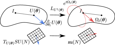
We now make the following observation: corresponds to a tangent vector on and generates the one-parameter subgroup such that
| (7) |
and
| (8) |
We sketch this procedure schematically in Fig. 1.
We now consider a typical variational setting, where we are interested in minimizing the following cost function:
| (9) |
where is some Hermitian operator and the initial state of the system. For simplicity we consider a circuit consisting of a single gate. Differentiating the cost function with respect to gives
| (10) |
Then, plugging in Eq. 8 we find,
where we used the skew-Hermitian property of the tangent vector . Note that Eq. 11 corresponds to a new circuit with the gate inserted before (see Fig. 2).
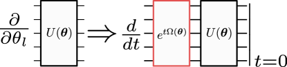
The gradient of this new circuit can be computed on quantum hardware with a generalized parameter-shift rule (GPSR) Wierichs2022grads ; Izmaylov2021grads ; Oleksandr2021grads . In Algorithm 1, we outline the entire algorithm for our gradient estimation and we denote the GPSR subroutine with gpsr. An alternative to the generalized shift rule is to decompose the effective generators and apply the original two-term parameter-shift rule to the constituents (see App. 3 for details). In Banchi2021measuringanalytic , the authors proposed the so-called stochastic parameter-shift rule for multivariate gates, which is based on the Monte Carlo approximation of an operator identity.
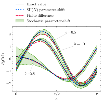
In Fig. 3 we consider a toy example using a random Hamiltonian on a single qubit and compare the exact derivative of an gate with our generalized parameter-shift method (Algorithm 1), the stochastic parameter-shift rule and the central finite difference derivative with shifts . In particular, we consider the gate with and compute the partial derivative with respect to over the range for three fixed values of on a state vector simulator (without shot noise). For the finite difference recipe we use , which we found to be a reasonable choice for a shot budget of shots per cost function evaluation (see App. 2). We observe that the generalized derivative reproduces the exact value while the finite difference derivative is slightly biased. This is to be expected because the latter is an approximate method. While decreasing the shift size reduces the deterministic approximation error, it leads to larger overall estimation errors in shot-based computations like on quantum computers (see App. 2 and e.g., bittel2022fast ). Finally, the stochastic parameter-shift rule yields an unbiased estimator for the exact derivative but has a finite variance, which we estimated using samples (see App. 1). We stress that this variance is a property of the differentiation method itself and not due to sampling on the quantum computer. All methods require two unique circuits per derivative but the stochastic shift rule needs additional circuits in order to suppress the variance. We provide the code for all our numerical experiments at our_code .
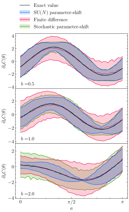
In addition, we compare the three methods in the presence of shot noise in Fig. 4. We show the means and single-shot errors estimated with shots, which we split over samples for the stochastic shift rule. We observe that the generalized shift rule systematically performs best. It is not only unbiased but also has the smallest variance. Note that for smaller parameters , the shift rule and the stochastic shift rule show very similar variances. This is because approaches the gate , which can be differentiated with the original parameter-shift rule, and both rules indeed reduce to the two-term shift rule for .
Finally, we note that Eq. 11 can is closely related to the Riemannian gradient on SchulteHerbruggen2010gradflow ; Wiersema2022riemann . However, instead of a gradient flow on a Lie group, we have defined a flow on the Lie algebra , which we retract back to the manifold via the exponential map. This subtle difference induces a different flow from the one, as we illustrate in App. C.
IV Comparison with decomposed unitaries
Previous parameterizations of unitaries consist of products of single-qubit gates and CNOTs Khaneja2001cartan ; kraus2001optimal ; Vatan2004opt2qubit ; vatan2004realization ; Vartiainen2004 ; Dalessandro2006decompuni . We refer to this parameterization as decomposed gates. On the other hand, Eq. 2 describes a general unitary by exponentiating a parameterization of the Lie algebra . Here, we investigate the effects of this alternative parameterization.
IV.1 Gate speed limit
First, we investigate a speed limit in terms of the gate time. We slightly modify the definition of Eq. 2 for a unitary evolution of the system, , to include a time ,
| (12) |
where is a normalized time-independent Hamiltonian (the imaginary unit is included in ). The normalization of is equivalent to the normalization of in Euclidean norm, see Lemma 3 in App. F. The normalization of the Hamiltonian (or, equivalently, ) means that the total path length covered by the evolution is directly proportional to the evolution time , since we are effectively setting the speed of the evolution to .
The Lie group can be turned into a Riemannian manifold by equipping it with the Hilbert-Schmidt inner product . A geodesic between two points on is a curve of minimal arc length. The unitary evolution , parameterized by , is a one-parameter subgroup that gives the geodesic (SchulteHerbruggen2010gradflow, , Theorem III.6) between the identity element at time to the final evolution at time . Using Lemma 4 (App. F), the length of the path after time is constant for time-independent normalized Hamiltonians with ,
| (13) |
and is the minimum time required to generate the evolution . For an initial state and final state , the Fubini-Study metric is used to find a minimum evolution time
| (14) |
giving the Mandelstam-Tamm bound for time-independent normalized Hamiltonians.
In practice, we may only have access to a restricted family of gates within , for example due to hardware limitations, in which case we require a decomposition of a desired gate in into gates from this family. Here we want to compute the additional evolution time required by such a decomposition. The simplest gate decomposition is to break the unitary into two terms, . The parameters and are also normalized Hamiltonians, i.e., they have the norm . The following theorem gives the additional evolution time of using the decomposed circuit over the geodesic evolution of a general gate.
Theorem 1.
Consider a general gate with geodesic evolution time together with a decomposition . Let be the total decomposed unitary evolution time. The additional time required by the decomposition is then given by
| (15) |
The proof of the theorem is in App. F. As expected, the additional time turns out to be positive, , for all . Due to the normalization of and , if , then . In this case, the restricted evolution is along the geodesic, , and . Theorem 1 gives the additional time for a decomposition into two gates. A decomposition into more gates would lead to an even greater evolution time. A corollary of Theorem 1 is that any circuit with multiple non-commuting layers of gates cannot be optimal in total time.
IV.2 Unbiased cost landscapes
An additional advantage of the gate is that it weighs all optimization directions equally. In contrast, a parameterization of in terms of a product of gates will create a bias in the parameter space. We illustrate this point with the following example. Consider the decomposed gate where and . This is the ZYZ decomposition. Using similar techniques as in App. F, we can rewrite to be parameterized in terms of the Lie algebra:
| (16) |
where and
| (17) |
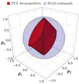
If we look at the components of , we see that the different directions in the Lie algebra are stretched or compressed as a result of the particular choice of parameterization. Consider the normalization for the ZYZ decomposition and for the gate. With each Hamiltonian term normalized to 1, the prefactor gives the evolution time. These choices of norm give equal total evolution times for the ZYZ decomposition and gate, , irrespective of the specific parameters chosen. In Fig. 5, we graphically illustrate the Lie algebra deformation by showing the surface for both the ZYZ decomposition and gate. Note that we have not considered any cost function here; the bias occurs at the level of the parameterization of a specific unitary.
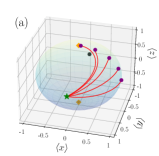
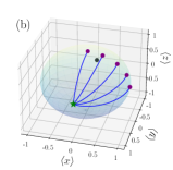
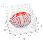
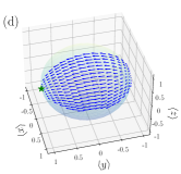
The effect of this bias is demonstrated in Fig. 6 for the simplest case of a single-qubit system with an gate. The optimal parameters of the circuit are those that produce the state that gives the minimum of the cost function (green star). We consider various initial parameters acting on the reference state . The corresponding training paths are shown for each initial parameter vector. The training paths for the decomposed ZYZ circuit are depicted in Fig. 6(a). As the initial parameter acting on the reference state (purple dots) moves closer to an unstable equilibrium point (orange diamond) the training path becomes increasingly suboptimal. At the unstable equilibrium the only gradient information is directly away from the instability rather than providing information about the direction towards the global minimum. This behavior is further illustrated by the gradient vector field on the Bloch sphere in Fig. 6(c). For the gate, we see in Fig. 6(b) that the optimization trajectories follow a direct path to the minimum.
IV.3 Numerical experiment
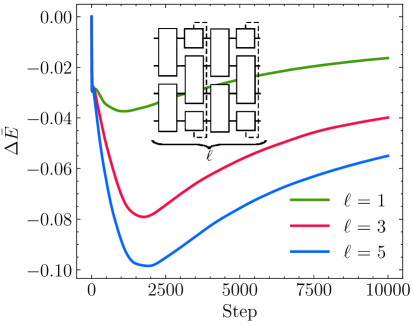
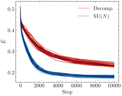
To investigate the effect on the performance of a typical optimization, we study how an gate compares with a decomposed gate in a larger circuit. In Fig. 7 we provide a non-trivial example, where we incorporate our gates into a circuit and show that it performs better than a decomposed gate on a set of random problem instances. We show the individual optimization trajectories in Fig. 8 which illustrate the faster optimization of gates compared to decomposed gates. Like for the examples in Fig. 3 and Fig. 4, we assume that there is no gate or measurement noise. Additionally, we assume that we can always implement the gate generated by , and have control over all Pauli operators . In practice, we typically only have access to a fixed set of generators . If this is the case, then we require a decomposition of in terms of the available operations on the device Khaneja2001cartan ; Dalessandro2006decompuni . All numerical results were obtained with PennyLane bergholm2018pennylane , and the gates can be accessed via the qml.SpecialUnitary class. Although we do not explore this here, one could make use of sparse optimization methods such as stochastic optimization sweke2020stochastic ; harrow2021low and frugal optimization arrasmith2020operator for the GPSR subroutine in our algorithm.
V Resource estimation
To obtain the partial derivative in Eq. 11 in practice we need to estimate the gradient of a circuit that contains a gate generated by . As noted in recent works on GPSR rules Wierichs2022grads ; Izmaylov2021grads ; Oleksandr2021grads , the computational cost of estimating this gradient is related to the spectral gaps of . In particular, if is the set of (possibly degenerate) eigenvalues of , we define the set of unique spectral gaps as where . Note that for distinct eigenvalues, the number of unique spectral gaps is at most . The total number of parameter-shifted circuits is then for a single partial derivative
Depending on the generator , this complexity can be improved. For instance, in Izmaylov2021grads , a Cartan decomposition is used to improve the number of circuits required from polynomial to linear or even logarithmic in . Additionally, in Wierichs2022grads , the different costs for first- and second-order gradients are determined for specific varational quantum algorithms like QAOA farhi2014quantum and RotoSolve vidal2018rotosolve ; parrish2019rotosolve ; nakanishi2020rotosolve ; Ostaszewski2021rotosolve . Finally, in Oleksandr2021grads , the computational cost of a variety of different gates is investigated in detail and the variance across the parameter regime is studied.
Instead of focusing on specific instances of the generator , we make more general observation about the computational complexity of parameter-shift gradient rules. In general, has full support on , since the consecutive applications of in Eq. 3 typically generate all of lloyd1996universal . However, for specific choices of , the application of to closes to form a subalgebra, called the dynamical Lie algebra of , that is contained in . These algebras are well-known in the context of quantum optimal control Albertini2001dynlie ; dalessandro2021 , and have recently been studied in the context of variational quantum algorithms larocca2022diagnosing ; larocca2021theory . For our purposes, we define the dynamical Lie algebra (DLA) as the subalgebra formed under the closure of the non-zero terms in under the commutator and ignore trivial subalgebras consisting of a single element. For example, given , , we have , since and successive commutators generate no new contributions. Note that for this example the DLA equals the full Lie algebra . In particular, for there is only one possible DLA, the one that spans . If , there exist several non-trivial cases. For example, in Schirmer2002dynlie explicit constructions are given for DLAs that span and . In a more recent work, the DLAs of several typical quantum many-body Hamiltonians are studied and their properties are used to prepare efficient time-evolution circuits Kokcu2021cartan . These Hamiltonians could be used as generators for gates.
Interestingly, if the DLA is maximal, i.e., there exists no smaller non-trivial subalgebra within , then the roots of the Lie algebra can be related directly to the computational cost of estimating the gradients in Eq. 11. We formally establish this connection with the following theorem:
Theorem 2.
The number of unique spectral gaps of is upper bounded by the number of roots of any maximal semi-simple DLA,
| (18) |
We provide the proof of Theorem 2 in App. G. We make use of the fact that any semisimple Lie algebra can be written as a direct sum of its weight spaces, which can be identified with its root system Serre2000complex . The number of roots can then be used to bound the total number of unique spectral gaps of . We can thus use Theorem 2 to assess the run time of Algorithm 1. We give several examples of gates in App. G together with the corresponding values of . Depending on the physical system or hardware that we are working with, we have to choose a representation for , which is a map . In Eq. 1 we chose this representation to be the tensor product of the fundamental representation, i.e., Pauli monomials. Note however, that Eq. 11 and Theorem 2 hold for any irreducible representation of .
Additionally, by connecting the spectral gaps to the root system of the DLA, we can make use of a beautiful result in representation theory: the classification of all maximal subalgebras of the classical Lie algebras dynkin1957american . Each root system can be uniquely identified with a particular subalgebra of a Lie algebra and it can be shown that there exist a finite number of root systems. Since a DLA is a subalgebra of , we can identify all possible DLAs and by extension all possible families of gates. We provide examples of this procedure in App. G.
VI Conclusion
We have proposed an alternative parameterization of general gates and a method of optimizing these gates in prototypical variational quantum algorithms. We have shown that our gates are more powerful in toy example settings, and motivated why we believe this is the case based on quantum speed-limit arguments. A natural extension of our work would be to test our method in experimental settings, both on gate-based quantum computers or quantum simulators Georgescu2014qsim ; ebadi2021quantum ; Scholl2022xxz . With regards to the latter, several methods have been investigated that could provide pulse-level optimization of energy cost functions ibrahim2022pulse ; meitei2020gate . This would obviate the need for a gate-based model of quantum computing to prepare specific states on quantum hardware. Instead, we work on the Hamiltonian level and control the system directly. Our algorithm could be applied to this setting as well, since we’re effectively learning the parameters of some fixed Hamiltonian.
We have shown that the gate in a circuit outperforms a decomposed gate. The number of parameters in our proposed gate requires parameters, and it is not clear for which problems one would rather have a deeper circuit with simple gates as opposed to a shallow circuit with more powerful gates. This also begs another question: will our gates suffer from barren plateaus mcclean2018barren ? It is likely that a circuit of 2-qubit gates that has linear depth in will lead to a circuit that forms an approximate 2-design, which will suffer from vanishing gradients. However, appropriate choices of the generators of our gate could keep the circuit in a polynomially scaling DLA of the entire circuit, which can avoid barren plateaus larocca2022diagnosing ; larocca2021theory . Additionally, we can consider parameter initialization strategies that can improve the optimization grant2019initialization ; skolik2021layerwise .
Finally, we believe that the connections between variational quantum circuits and representation theory merit further investigation. We connected the classification of all gates with the classification of semisimple Lie algebras. However, this could possibly be extended to a classification of all variational quantum circuits based on the DLA of an ansatz. It seems that the tools to provide such a classification are available and could provide one with a method to assess the trainability and expressivity of variational circuits without explicitly referring to specific ansätze.
VII Acknowledgements
We want to thank Los Alamos National Lab for their hospitality during the Quantum Computing Summer School where the initial stages of this project took place. RW wants to thank Lex Kemper and Efekan Kökcü for discussions on the subject of dynamical Lie algebras and Matt Duchenes for his suggestions with regards to the experimental implications of our work. DL acknowledges support from the EPSRC Centre for Doctoral Training in Delivering Quantum Technologies, grant ref. EP/S021582/1. JFCA acknowledges support from the Natural Sciences and Engineering Research Council (NSERC), the Shared Hierarchical Academic Research Computing Network (SHARCNET), Compute Canada, and the Canadian Institute for Advanced Research (CIFAR) AI chair program. Resources used in preparing this research were provided, in part, by the Province of Ontario, the Government of Canada through CIFAR, and companies sponsoring the Vector Institute https://vectorinstitute.ai/#partners.
References
- (1) M. Cerezo, Andrew Arrasmith, Ryan Babbush, Simon C. Benjamin, Suguru Endo, Keisuke Fujii, Jarrod R. McClean, Kosuke Mitarai, Xiao Yuan, Lukasz Cincio, and Patrick J. Coles. “Variational quantum algorithms”. Nature Reviews Physics 3, 625–644 (2021).
- (2) Jules Tilly, Hongxiang Chen, Shuxiang Cao, Dario Picozzi, Kanav Setia, Ying Li, Edward Grant, Leonard Wossnig, Ivan Rungger, George H. Booth, and Jonathan Tennyson. “The Variational Quantum Eigensolver: A review of methods and best practices”. Physics Reports 986, 1–128 (2022).
- (3) Jun Li, Xiaodong Yang, Xinhua Peng, and Chang-Pu Sun. “Hybrid Quantum-Classical Approach to Quantum Optimal Control”. Phys. Rev. Lett. 118, 150503 (2017).
- (4) K. Mitarai, M. Negoro, M. Kitagawa, and K. Fujii. “Quantum circuit learning”. Phys. Rev. A 98, 032309 (2018).
- (5) Maria Schuld, Ville Bergholm, Christian Gogolin, Josh Izaac, and Nathan Killoran. “Evaluating analytic gradients on quantum hardware”. Phys. Rev. A 99, 032331 (2019).
- (6) Gavin E. Crooks. “Gradients of parameterized quantum gates using the parameter-shift rule and gate decomposition” (2019) arXiv:1905.13311.
- (7) Artur F. Izmaylov, Robert A. Lang, and Tzu-Ching Yen. “Analytic gradients in variational quantum algorithms: Algebraic extensions of the parameter-shift rule to general unitary transformations”. Phys. Rev. A 104, 062443 (2021).
- (8) David Wierichs, Josh Izaac, Cody Wang, and Cedric Yen-Yu Lin. “General parameter-shift rules for quantum gradients”. Quantum 6, 677 (2022).
- (9) Oleksandr Kyriienko and Vincent E. Elfving. “Generalized quantum circuit differentiation rules”. Phys. Rev. A 104, 052417 (2021).
- (10) Dirk Oliver Theis. “"Proper" Shift Rules for Derivatives of Perturbed-Parametric Quantum Evolutions” (2022) arXiv:2207.01587.
- (11) Lucas Slattery, Benjamin Villalonga, and Bryan K. Clark. “Unitary block optimization for variational quantum algorithms”. Phys. Rev. Research 4, 023072 (2022).
- (12) Jin-Guo Liu, Yi-Hong Zhang, Yuan Wan, and Lei Wang. “Variational quantum eigensolver with fewer qubits”. Phys. Rev. Research 1, 023025 (2019).
- (13) Abhinav Kandala, Antonio Mezzacapo, Kristan Temme, Maika Takita, Markus Brink, Jerry M. Chow, and Jay M. Gambetta. “Hardware-efficient variational quantum eigensolver for small molecules and quantum magnets”. Nature 549, 242–246 (2017).
- (14) Navin Khaneja and Steffen J. Glaser. “Cartan decomposition of and control of spin systems”. Chemical Physics 267, 11–23 (2001).
- (15) Barbara Kraus and Juan I Cirac. “Optimal creation of entanglement using a two-qubit gate”. Physical Review A 63, 062309 (2001).
- (16) Farrokh Vatan and Colin Williams. “Optimal quantum circuits for general two-qubit gates”. Phys. Rev. A 69, 032315 (2004).
- (17) Farrokh Vatan and Colin P Williams. “Realization of a general three-qubit quantum gate” (2004). arXiv:quant-ph/0401178.
- (18) Juha J. Vartiainen, Mikko Möttönen, and Martti M. Salomaa. “Efficient Decomposition of Quantum Gates”. Phys. Rev. Lett. 92, 177902 (2004).
- (19) Domenico D’Alessandro and Raffaele Romano. “Decompositions of unitary evolutions and entanglement dynamics of bipartite quantum systems”. Journal of Mathematical Physics 47, 082109 (2006).
- (20) Alwin Zulehner and Robert Wille. “Compiling SU(4) Quantum Circuits to IBM QX Architectures”. In Proceedings of the 24th Asia and South Pacific Design Automation Conference. Page 185–190. ASPDAC ’19New York, NY, USA (2019). Association for Computing Machinery.
- (21) B. Foxen, C. Neill, A. Dunsworth, P. Roushan, B. Chiaro, A. Megrant, J. Kelly, Zijun Chen, K. Satzinger, R. Barends, F. Arute, K. Arya, R. Babbush, D. Bacon, J. C. Bardin, S. Boixo, D. Buell, B. Burkett, Yu Chen, R. Collins, E. Farhi, A. Fowler, C. Gidney, M. Giustina, R. Graff, M. Harrigan, T. Huang, S. V. Isakov, E. Jeffrey, Z. Jiang, D. Kafri, K. Kechedzhi, P. Klimov, A. Korotkov, F. Kostritsa, D. Landhuis, E. Lucero, J. McClean, M. McEwen, X. Mi, M. Mohseni, J. Y. Mutus, O. Naaman, M. Neeley, M. Niu, A. Petukhov, C. Quintana, N. Rubin, D. Sank, V. Smelyanskiy, A. Vainsencher, T. C. White, Z. Yao, P. Yeh, A. Zalcman, H. Neven, and J. M. Martinis. “Demonstrating a Continuous Set of Two-Qubit Gates for Near-Term Quantum Algorithms”. Phys. Rev. Lett. 125, 120504 (2020).
- (22) E Groeneveld. “A reparameterization to improve numerical optimization in multivariate REML (co) variance component estimation”. Genetics Selection Evolution 26, 537–545 (1994).
- (23) Tapani Raiko, Harri Valpola, and Yann LeCun. “Deep learning made easier by linear transformations in perceptrons”. In Artificial intelligence and statistics. Pages 924–932. PMLR (2012). url: https://proceedings.mlr.press/v22/raiko12.html.
- (24) Sergey Ioffe and Christian Szegedy. “Batch normalization: Accelerating deep network training by reducing internal covariate shift”. In International conference on machine learning. Pages 448–456. PMLR (2015).
- (25) Tim Salimans and Durk P Kingma. “Weight normalization: A simple reparameterization to accelerate training of deep neural networks”. In Advances in neural information processing systems. Volume 29. (2016).
- (26) Robert Price. “A useful theorem for nonlinear devices having Gaussian inputs”. IRE Transactions on Information Theory 4, 69–72 (1958).
- (27) Danilo Jimenez Rezende, Shakir Mohamed, and Daan Wierstra. “Stochastic backpropagation and approximate inference in deep generative models”. In International conference on machine learning. Pages 1278–1286. PMLR (2014). url: https://proceedings.mlr.press/v32/rezende14.html.
- (28) Diederik P. Kingma and Max Welling. “Auto-Encoding Variational Bayes”. In Yoshua Bengio and Yann LeCun, editors, 2nd International Conference on Learning Representations, ICLR 2014, Banff, AB, Canada, April 14-16, 2014, Conference Track Proceedings. (2014). url: http://arxiv.org/abs/1312.6114.
- (29) Brian C Hall. “Lie groups, Lie algebras, and representations”. Springer. (2013). 2nd edition.
- (30) William Fulton and Joe Harris. “Representation theory: a first course”. Volume 129. Springer Science & Business Media. (2013).
- (31) W. Rossmann. “Lie Groups: An Introduction Through Linear Groups”. Oxford graduate texts in mathematics. Oxford University Press. (2002). 5th edition. url: https://books.google.ca/books?id=bAjulQ65W-UC.
- (32) Jean-Pierre Serre. “Lie algebras and Lie groups: 1964 lectures given at Harvard University”. Springer. (2009).
- (33) Jiaqi Leng, Yuxiang Peng, Yi-Ling Qiao, Ming Lin, and Xiaodi Wu. “Differentiable Analog Quantum Computing for Optimization and Control” (2022). arXiv:2210.15812.
- (34) R. M. Wilcox. “Exponential Operators and Parameter Differentiation in Quantum Physics”. Journal of Mathematical Physics 8, 962–982 (1967). arXiv:https://doi.org/10.1063/1.1705306.
- (35) E. T. Whittaker. “XVIII.—On the Functions which are represented by the Expansions of the Interpolation-Theory”. Proceedings of the Royal Society of Edinburgh 35, 181–194 (1915).
- (36) James Bradbury, Roy Frostig, Peter Hawkins, Matthew James Johnson, Chris Leary, Dougal Maclaurin, George Necula, Adam Paszke, Jake VanderPlas, Skye Wanderman-Milne, and Qiao Zhang (2018). code: google/jax.
- (37) Adam Paszke, Sam Gross, Francisco Massa, Adam Lerer, James Bradbury, Gregory Chanan, Trevor Killeen, Zeming Lin, Natalia Gimelshein, Luca Antiga, et al. “Pytorch: An imperative style, high-performance deep learning library”. In Advances in neural information processing systems. Volume 32. (2019).
- (38) Martín Abadi, Ashish Agarwal, Paul Barham, Eugene Brevdo, Zhifeng Chen, Craig Citro, Greg S. Corrado, Andy Davis, Jeffrey Dean, Matthieu Devin, Sanjay Ghemawat, Ian Goodfellow, Andrew Harp, Geoffrey Irving, Michael Isard, Yangqing Jia, Rafal Jozefowicz, Lukasz Kaiser, Manjunath Kudlur, Josh Levenberg, Dandelion Mané, Rajat Monga, Sherry Moore, Derek Murray, Chris Olah, Mike Schuster, Jonathon Shlens, Benoit Steiner, Ilya Sutskever, Kunal Talwar, Paul Tucker, Vincent Vanhoucke, Vijay Vasudevan, Fernanda Viégas, Oriol Vinyals, Pete Warden, Martin Wattenberg, Martin Wicke, Yuan Yu, and Xiaoqiang Zheng (2015). code: https://www.tensorflow.org/.
- (39) A JAX implementation of the matrix exponential that can be differentiated via automatic differentiation: https://jax.readthedocs.io/en/latest/_autosummary/jax.scipy.linalg.expm.html.
- (40) Awad H Al-Mohy and Nicholas J Higham. “A new scaling and squaring algorithm for the matrix exponential”. SIAM Journal on Matrix Analysis and Applications 31, 970–989 (2010).
- (41) Leonardo Banchi and Gavin E. Crooks. “Measuring Analytic Gradients of General Quantum Evolution with the Stochastic Parameter Shift Rule”. Quantum 5, 386 (2021).
- (42) Lennart Bittel, Jens Watty, and Martin Kliesch. “Fast gradient estimation for variational quantum algorithms” (2022). arXiv:2210.06484.
- (43) Roeland Wiersema, Dylan Lewis, David Wierichs, Juan Carrasquilla, and Nathan Killoran (2023). code: dwierichs/Here-comes-the-SUN.
- (44) Thomas Schulte-Herbrüggen, Steffen j. Glaser, Gunther Dirr, and Uwe Helmke. “Gradient Flows for Optimization in Quantum Information and Quantum Dynamics: Foundations and Applications”. Reviews in Mathematical Physics 22, 597–667 (2010).
- (45) Roeland Wiersema and Nathan Killoran. “Optimizing quantum circuits with Riemannian gradient flow” (2022) arXiv:2202.06976.
- (46) Ville Bergholm, Josh Izaac, Maria Schuld, Christian Gogolin, M Sohaib Alam, Shahnawaz Ahmed, Juan Miguel Arrazola, Carsten Blank, Alain Delgado, Soran Jahangiri, et al. “Pennylane: Automatic differentiation of hybrid quantum-classical computations” (2018). arXiv:1811.04968.
- (47) Ryan Sweke, Frederik Wilde, Johannes Meyer, Maria Schuld, Paul K. Faehrmann, Barthélémy Meynard-Piganeau, and Jens Eisert. “Stochastic gradient descent for hybrid quantum-classical optimization”. Quantum 4, 314 (2020).
- (48) Aram W. Harrow and John C. Napp. “Low-Depth Gradient Measurements Can Improve Convergence in Variational Hybrid Quantum-Classical Algorithms”. Phys. Rev. Lett. 126, 140502 (2021).
- (49) Andrew Arrasmith, Lukasz Cincio, Rolando D Somma, and Patrick J Coles. “Operator sampling for shot-frugal optimization in variational algorithms” (2020). arXiv:2004.06252.
- (50) Edward Farhi, Jeffrey Goldstone, and Sam Gutmann. “A quantum approximate optimization algorithm” (2014). arXiv:1411.4028.
- (51) Javier Gil Vidal and Dirk Oliver Theis. “Calculus on parameterized quantum circuits” (2018). arXiv:1812.06323.
- (52) Robert M Parrish, Joseph T Iosue, Asier Ozaeta, and Peter L McMahon. “A Jacobi diagonalization and Anderson acceleration algorithm for variational quantum algorithm parameter optimization” (2019). arXiv:1904.03206.
- (53) Ken M. Nakanishi, Keisuke Fujii, and Synge Todo. “Sequential minimal optimization for quantum-classical hybrid algorithms”. Phys. Rev. Res. 2, 043158 (2020).
- (54) Mateusz Ostaszewski, Edward Grant, and Marcello Benedetti. “Structure optimization for parameterized quantum circuits”. Quantum 5, 391 (2021).
- (55) Seth Lloyd. “Universal quantum simulators”. Science 273, 1073–1078 (1996).
- (56) F. Albertini and D. D’Alessandro. “Notions of controllability for quantum mechanical systems”. In Proceedings of the 40th IEEE Conference on Decision and Control (Cat. No.01CH37228). Volume 2, pages 1589–1594 vol.2. (2001).
- (57) Domenico d’Alessandro. “Introduction to quantum control and dynamics”. Chapman and hall/CRC. (2021). 2nd edition.
- (58) Martin Larocca, Piotr Czarnik, Kunal Sharma, Gopikrishnan Muraleedharan, Patrick J. Coles, and M. Cerezo. “Diagnosing Barren Plateaus with Tools from Quantum Optimal Control”. Quantum 6, 824 (2022).
- (59) Martin Larocca, Nathan Ju, Diego García-Martín, Patrick J Coles, and Marco Cerezo. “Theory of overparametrization in quantum neural networks” (2021). arXiv:2109.11676.
- (60) S G Schirmer, I C H Pullen, and A I Solomon. “Identification of dynamical Lie algebras for finite-level quantum control systems”. Journal of Physics A: Mathematical and General 35, 2327 (2002).
- (61) Efekan Kökcü, Thomas Steckmann, J. K. Freericks, Eugene F. Dumitrescu, and Alexander F. Kemper. “Fixed Depth Hamiltonian Simulation via Cartan Decomposition” (2021). arXiv:2104.00728.
- (62) Jean-Pierre Serre. “Complex semisimple Lie algebras”. Springer Science & Business Media. (2000). 1st edition.
- (63) Eugene Borisovich Dynkin. “American Mathematical Society Translations: Five Papers on Algebra and Group Theory”. American Mathematical Society. (1957).
- (64) I. M. Georgescu, S. Ashhab, and Franco Nori. “Quantum simulation”. Rev. Mod. Phys. 86, 153–185 (2014).
- (65) Sepehr Ebadi, Tout T Wang, Harry Levine, Alexander Keesling, Giulia Semeghini, Ahmed Omran, Dolev Bluvstein, Rhine Samajdar, Hannes Pichler, Wen Wei Ho, et al. “Quantum phases of matter on a 256-atom programmable quantum simulator”. Nature 595, 227–232 (2021).
- (66) P. Scholl, H. J. Williams, G. Bornet, F. Wallner, D. Barredo, L. Henriet, A. Signoles, C. Hainaut, T. Franz, S. Geier, A. Tebben, A. Salzinger, G. Zürn, T. Lahaye, M. Weidemüller, and A. Browaeys. “Microwave Engineering of Programmable Hamiltonians in Arrays of Rydberg Atoms”. PRX Quantum 3, 020303 (2022).
- (67) Mohannad Ibrahim, Hamed Mohammadbagherpoor, Cynthia Rios, Nicholas T Bronn, and Gregory T Byrd. “Pulse-Level Optimization of Parameterized Quantum Circuits for Variational Quantum Algorithms” (2022). arXiv:2211.00350.
- (68) Oinam Romesh Meitei, Bryan T Gard, George S Barron, David P Pappas, Sophia E Economou, Edwin Barnes, and Nicholas J Mayhall. “Gate-free state preparation for fast variational quantum eigensolver simulations: ctrl-vqe” (2020). arXiv:2008.04302.
- (69) Jarrod R McClean, Sergio Boixo, Vadim N Smelyanskiy, Ryan Babbush, and Hartmut Neven. “Barren plateaus in quantum neural network training landscapes”. Nature communications 9, 1–6 (2018).
- (70) Edward Grant, Leonard Wossnig, Mateusz Ostaszewski, and Marcello Benedetti. “An initialization strategy for addressing barren plateaus in parametrized quantum circuits”. Quantum 3, 214 (2019).
- (71) Andrea Skolik, Jarrod R McClean, Masoud Mohseni, Patrick van der Smagt, and Martin Leib. “Layerwise learning for quantum neural networks”. Quantum Machine Intelligence 3, 1–11 (2021).
- (72) Rüdiger Achilles and Andrea Bonfiglioli. “The early proofs of the theorem of Campbell, Baker, Hausdorff, and Dynkin”. Archive for History of Exact Sciences 66, 295–358 (2012).
- (73) Mario Lezcano-Casado and David Martınez-Rubio. “Cheap orthogonal constraints in neural networks: A simple parametrization of the orthogonal and unitary group”. In International Conference on Machine Learning. Pages 3794–3803. PMLR (2019).
- (74) Andrea Mari, Thomas R. Bromley, and Nathan Killoran. “Estimating the gradient and higher-order derivatives on quantum hardware”. Phys. Rev. A 103, 012405 (2021).
- (75) Benjamin Russell and Susan Stepney. “Geometric Methods for Analysing Quantum Speed Limits: Time-Dependent Controlled Quantum Systems with Constrained Control Functions”. In Giancarlo Mauri, Alberto Dennunzio, Luca Manzoni, and Antonio E. Porreca, editors, Unconventional Computation and Natural Computation. Pages 198–208. Lecture Notes in Computer ScienceBerlin, Heidelberg (2013). Springer.
- (76) James E Humphreys. “Introduction to Lie algebras and representation theory”. Volume 9. Springer Science & Business Media. (2012).
Supplemental Materials
A and its Lie algebra
Consider the special unitary Lie group :
| (A1) |
In general, quantum gates belong to the unitary group , which drops the determinant 1 condition and thus allows for an additional global phase. Restricting ourselves to therefore is physically equivalent. Consider a curve , such that and . If we differentiate the unitarity condition with respect to , we obtain
| (A2) | ||||
| (A3) | ||||
| (A4) |
and so we find that , i.e., is a skew-Hermitian matrix. The matrices from all such curves are elements of the Lie algebra
| (A5) |
The second condition, , can be found by realizing that the Lie algebra is connected to a Lie group via the exponential map: , and and so . Instead of considering a curve going through the identity at , we can consider a curve going through a point with directional derivative . All curves with directional derivative at the point form an equivalence class. The set of these equivalence classes forms a vector space called the tangent space at the point , and in particular we may identify . The group product , i.e., left multiplication by an element , is a local homeomorphism, which induces a linear map between two tangent spaces: where . is called the differential of . If we take to be the identity, then we see that we can move from the tangent space at the identity to the tangent space at any point in by left multiplication of the group . Hence the tangent space at is given by
| (A6) |
B The exponential map and its gradient
The following is due to rossmann2002lie (Chapter 1, Theorem 5). Let be a matrix Lie group with a corresponding Lie algebra . Define conjugation by to be the transformation given by . Note that is an (inner) automorphism of , since it is a isomorphism from onto itself. Let be the exponential map from the Lie algebra to the group. Taking and , the differential of the conjugation map at the identity is
| (B1) |
which maps an element of the Lie algebra to another element of the Lie algebra. This map is called the adjoint representation and takes . Given , we compute
| (B2) | ||||
| (B3) | ||||
| (B4) | ||||
| (B5) |
The operator is the Lie bracket on , which for our purposes will be the standard commutator. It now follows that
| (B6) | ||||
| (B7) | ||||
| (B8) |
With the boundary condition we find that the above differential equation is solved by
| (B9) |
at . Consider now the following parameterized matrix function ,
| (B10) |
where is a curve on . We then find
| (B11) | ||||
| (B12) | ||||
| (B13) | ||||
| (B14) |
Then with equation Eq. B9, we find
| (B15) |
Using that , we find by integration
| (B16) |
Estimating the above integral forms the basis of the stochastic parameter-shift rule (see App. 1). Continuing,
| (B17) | ||||
| (B18) | ||||
| (B19) |
Hence we see that
| (B20) |
which gives Eq. 3.
Note that at this point the Baker-Campbell-Hausdorff formula can be derived with Eq. B20 by considering the derivative of
| (B21) |
and subsequent integration of the derivative of Achilles2022bch .
C Connection between Riemannian and standard gradient flow on
Here, we highlight the connection between the Riemannian gradient flow and Eq. 11 SchulteHerbruggen2010gradflow ; Wiersema2022riemann . We take the Hilbert-Schmidt inner product as a Riemannian metric on and write the cost as
| (C1) |
The differential of the cost , evaluated at the point , where and , is then
| (C2) | ||||
| (C3) | ||||
| (C4) | ||||
| (C5) | ||||
| (C6) | ||||
| (C7) |
via the chain rule and using that . The compatibility condition for the Riemannian gradient tells us that
| (C8) |
Hence we can identify
| (C9) |
with the corresponding gradient flow
| (C10) |
Next, we follow the results of lezcano2019cheap in our notation. Consider the cost function
| (C11) |
where . Note that although the minimum of the function is unchanged, the parameterization of a unitary via the Lie algebra changes the resulting gradient flow. To see this, we consider again the differential,
| (C12) | ||||
| (C13) |
where now and . We can now make use of the result in Eq. B20,
| (C14) | ||||
| (C15) |
to obtain
| (C16) |
Using that and , we then have
| (C17) | ||||
| (C18) | ||||
| (C19) |
Hence the gradient on is
| (C21) |
We therefore see that only when do we obtain the Riemannian gradient; hence only if where is abelian. The optimization path followed by optimizing the parameters of an gate is thus different from the one following a Riemannian gradient descent on .
D The generalized parameter-shift rule
When using our gate in an application that involves gradient-based optimization, like demonstrated in the numerical experiments in this work, we require calculating the partial derivatives in Eq. 11. Here we provide the details for how this can be achieved in practice via the generalized parameter-shift rule (GPSR) Wierichs2022grads ; Izmaylov2021grads ; Oleksandr2021grads . Without loss of generality, we rewrite the cost function in Eq. 9 as
| (D1) |
where we absorbed the rest of the circuit into , and fixed any other parameters in the circuit. Computing the derivative of Eq. D1 with respect to is equivalent to the problem of finding the gradient in Eq. 11 at . For the numerical experiments in this paper we make use of the particular implementation of the GPSR in Oleksandr2021grads as well as the alternative method outlined in App. 3.
The skew-Hermitian operator in Eq. D1 has (possibly degenerate) eigenvalues . We define the set of unique spectral gaps as where . Note that for distinct eigenvalues, the number of unique spectral gaps is bounded via . We relabel every unique spectral gap with an integer, i.e. we write , and define the corresponding vector . We pick a set of parameter shifts that are equidistant and create a vector of shifts where
| (D2) |
Next, we create the length cost vector and the matrix
| (D3) |
We then calculate the coefficient vector as
| (D4) |
which finally gives the gradient
| (D5) |
Since the final gradient is exact, finite shot estimates of all ’s will produce an unbiased estimate of ,
| (D6) |
where we pulled out and since they are constant. The difficulty of obtaining an accurate estimate of the gradient is determined by the variance of this estimator, which is given by
| (D7) |
where we used to emphasize that the squares are taken elementwise. We assume that the estimates for each shifted circuit obey normal statistics and so since these are independent, we can write
| (D8) |
where is the variance of the cost for each shifted circuit. If we assume that the dependence of on the shifts is mild, i.e., then the total variance will only depend on the prefactor. Setting the estimate then finally gives
| (D9) |
One can minimize this quantity with respect to to find the optimal set of shifts for the gradient estimation Oleksandr2021grads .
E Alternative differentiation of gates
In this section we summarize a number of alternative differentiation techniques that may be applied to the presented gates. In particular, we discuss the stochastic parameter-shift rule, which was created for multi-parameter gates, finite differences as a standard tool in numerical differentiation, as well as an alternative to the general parameter-shift rule above which also exploits the notion of effective generators.
1 The Stochastic parameter-shift rule
The stochastic parameter-shift rule Crooks2019grads relies on the following operator identity Wilcox1967exponential
| (E1) |
for any bounded operator . We now fix all parameters for and rewrite the cost in Eq. 9 as
| (E2) |
Then, if we take to be the operator we can construct the gradient of Eq. E2 as
| (E3) |
where
| (E4) | ||||
| (E5) |
Hence, similar to our method, the gradient evaluation requires adding gates to the circuit and evaluating the new circuit. However, the stochastic parameter-shift rule comes at a significant cost: the evaluation of the integral in Eq. E3. In practice, one approximates this integral by sampling values of uniformly in the interval and then calculating the costs with a finite-shot estimate. Although this produces an unbiased estimator, we find that the variance of this estimator is larger than ours, see Fig. 4. In addition, this method leads to a bigger number of unique circuits to compute the derivative, increasing the compilation overhead for both hardware and simulator implementations.
2 Finite differences
Finite differences are widely used to differentiate functions numerically. We briefly discuss this method in the context of variational quantum computation (VQC) and refer the reader to recent works comparing and optimizing differentiation techniques for VQC mari2021estimating ; bittel2022fast .
In particular, we consider the central difference recipe
| (E6) |
where is a freely chosen shift parameter and is the th canonical basis vector. This recipe is an approximation of , making the corresponding estimator on a shot-based quantum computer biased. This bias, which depends on , has to be traded off against the variance of the estimator, which grows approximately with .
In classical computations, the numerical precision cutoff plays the role of the variance. Due to the high precision in classical computers, this leads to optimal shifts , which allows treating the bias to leading order in and thus enables rough estimates of the optimal in advance. On a quantum computer, however, the variance typically is more than ten orders of magnitude larger, leading to a very different , which furthermore depends on the function and derivative values. As a consequence, shifts of become a reasonable choice, highlighting the similarity of the central difference recipe to the two-term parameter-shift rule mari2021estimating .
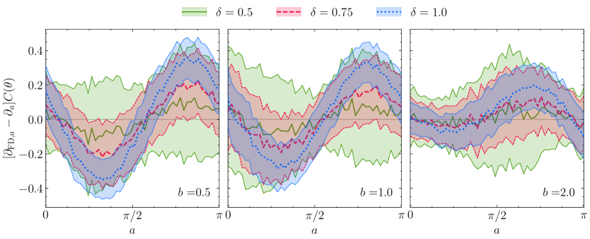
As a demonstration of the above, and in preparation for the numerical experiments shown in Figs. 3 and 4, we compute the central difference gradient for a random single-qubit Hamiltonian, a single gate and . For this, we evaluate the mean and standard error times and show the difference to the exact derivative in Fig. E1. As expected, we observe that the bias increases with and that the variance is suppressed with larger . We determine to be a reasonable choice for the purpose of the demonstration in Figs. 3 and 4, but stress that for any other circuit, qubit count, Hamiltonian, and even for a different parameter position for this circuit, the optimal shift size needs to be determined anew.
3 Decomposing effective generators for differentiation
In Algorithm 1 we suggest to use the generalized parameter-shift rule Izmaylov2021grads ; Wierichs2022grads ; Oleksandr2021grads in order to compute the partial derivatives independently. In addition, Theorem 2 bounds the number of frequencies occurring in the univariate auxiliary cost function and the corresponding number of parameter shifts required during differentiation.
Realizing the shift rule requires us to implement not only —which is necessary to compute itself—but also the gate for shift values and each separately. Alternatively, we may follow the approach to decompose all effective generators and compute the derivative as a linear combination of the derivatives for simpler auxiliary gates, similar to Izmaylov2021grads . In particular, we again choose the Pauli basis of for this decomposition.
Decompose the effective generators as
| (E7) |
Note that the coefficients are purely imaginary due to the skew-Hermiticity of . The partial derivative we are interested in can then be written as
| (E8) | ||||
| (E9) | ||||
| (E10) | ||||
| (E11) |
Here we abbreviated and wrote for the cost function with a rotation gate with parameter about inserted before . This modified cost function can be differentiated with respect to using the original two-term parameter-shift rule, as the inserted gate is generated by (the multiple of) a Pauli string.
The above linear combination of Pauli rotation derivatives can be reused for all partial derivatives, so that the full gradient for one gate is given by
| (E12) | ||||
| (E13) |
So far we did not discuss the number of Pauli strings occurring in the decomposition of the generators . As can be seen from Eq. 6 and our definition of the DLA in Section V, this number is bounded by the size of the DLA, and we again remark that this bound will be saturated for most values of . As two shifts are required for each Pauli rotation, the gradient can thus be computed using circuits, using Pauli rotations from the DLA and, e.g., shift angles .
As we only required a linear decomposition of , any other basis for the DLA may be used as well, potentially allowing for fewer shifted circuits or different inserted gates that may be more convenient to realize on hardware.
F Gate speed limit
The following Lemmas are used in Section IV.1.
Lemma 3.
For Hamiltonians of the form , where are strings of Pauli operators, .
Proof.
All Pauli strings are orthonormal with respect to the trace inner product, . Using this gives
| (F1) | ||||
| (F2) | ||||
| (F3) |
∎
Lemma 4.
The length of a smooth curve on the Riemannian manifold , with metric , for a time-independent Hamiltonian after a fixed time only depends on the norm of and .
Proof.
The unitary evolution of , parameterized by , corresponds to a smooth curve on with length according to the Riemannian metric, Russell2013Geometric . Integrating over the metric norm through the tangent spaces from to final time gives the path length,
| (F4) | ||||
| (F5) | ||||
| (F6) |
where . From Schrödinger evolution,
| (F7) |
we find
| (F8) |
for time-independent Hamiltonians. Therefore for all Hamiltonians with fixed norm , the path distance travelled after time is the same regardless of the specific unitary evolution. ∎
1 Proof of Theorem 1
The decomposed circuit is given by two unitary evolutions. Each individual evolution is a rotation such that only a single basis element of the whole Lie algebra is required. With two rotations, the overall evolution is an element of . The corresponding subalgebra is spanned by three basis elements—the three Pauli matrices for example. The two rotations can be represented as lying on a Bloch sphere. A unitary transformation, , can therefore be applied to the evolution such that for
| (F9) |
where , with and parameterizing the rotations. By construction is normalised for all parameters and . The same transformation defines and gives the same relationship . This is straightfoward to show
| (F10) | ||||
| (F11) | ||||
| (F12) | ||||
| (F13) |
We have
| (F14) |
where we choose , and . These basis elements of generate the group . Exponentiation therefore gives the closed-form expression
| (F15) | ||||
| (F16) |
where . By the group composition law of , the product of two exponentials in also gives a closed-form expression,
| (F17) |
Collecting terms gives
| (F18) |
The total evolution is
| (F19) | ||||
| (F20) |
By comparison of Eqs. (F18) and (F20), we find
| (F21) |
and
| (F22) |
The additional evolution time is , with . Due to the invariance of the scalar product, , we arrive at the expression in the statement of the theorem.
G Unique spectral gaps of Dynamical Lie Algebras
1 Proof of Theorem 2
In the following we set to be a semisimple Lie algebra. A subspace is called a subalgebra if it is closed under the Lie bracket, i.e., if , . Since is a semisimple Lie algebra, it always contains a subalgebra called a Cartan subalgebra hall2013lie (Chapter 7, Definition 7.10).
Definition 1.
A Cartan subalgebra of is a subalgebra that satisfies the following conditions:
-
1.
For all , .
-
2.
For all , if for all , then .
The first condition tells us that is a commutative subalgebra of , while the second condition says that is maximal, i.e., there is no larger commutative subalgebra. The first step in proving Theorem 2 is to make use of the following result Serre2000complex (Chapter VI, Theorem 1):
Theorem 5.
If is a semisimple Lie algebra, we can write as a direct sum of the weight spaces :
| (G1) |
where
| (G2) |
and are functionals on . That is, a weight space is a subspace of on which the action of the adjoint representation of is described by a functional (and scalar multiplication).
Since
| (G3) |
we find that and hence
| (G4) |
We therefore find that
| (G5) |
We can thus relate the dimensionality of a Lie algebra to the dimensionality of its Cartan subalgebra and its weight spaces. The second step of the proof relies on identifying the unique spectral gaps of with the weight spaces . To achieve this, we will construct the linear operator and apply it to the eigenbasis of to show that the maps can be identified with the spectral gaps of .
Consider an element , where is a non-trivial subalgebra and is a Cartan subalgebra of . Since is the Lie algebra of a maximally abelian group, we can represent elements of by diagonal matrices. Since is skew-Hermitian, there exists a unitary that diagonalizes , i.e., with . Here, is the matrix with columns equal to the eigenvectors of with corresponding eigenvalues . We can thus always choose a basis for such that is diagonal. If is non-degenerate, then it must be full rank, and therefore an element of . All Cartan algebras are equivalent up to conjugacy, hence we can choose the matrix to be the diagonal matrix containing the eigenvalues of to represent the Cartan subalgebra . We now take to be the matrix with entries equal to 1 and all other entries to 0. Define the operator
| (G6) |
and apply to it:
| (G7) | ||||
| (G8) | ||||
| (G9) | ||||
| (G10) |
This means that has the eigenvectors with corresponding eigenvalues humphreys2012introduction . From App. 5, we see that each weight space can be uniquely identified through the eigenvalues of . These eigenvalues are called the roots of the Lie algebra and are the main tool in the classification of semisimple Lie algebras dynkin1957american . We define the set of all roots as
| (G11) |
Since the dimensionality of each weight space is one Serre2000complex (Chapter VI, Theorem 2(a)), we can see that
| (G12) |
Therefore,
| (G13) |
We now set . If we take the absolute value of the elements of , we can identify , where the factor is to account for double counting of the spectral gaps. Since can be degenerate in general, we obtain the inequality . In practice, will almost always saturate this bound and this will be an equality. With this, the proof of Theorem 2 is completed.
2 Examples
Here, we give several examples of maximal DLAs and their corresponding value of . Analogous to the main text, we choose the Pauli representation but these results should hold for any irreducible representation of .
-
1.
: For a 1-qubit system, there are no non-trivial subalgebras, hence we can only look at the full special unitary Lie algebra . Any that consists of two Pauli operators will generate this algebra, e.g.,
(G14) will give . A Cartan subalgebra of is given by . We therefore find that and and so . Hence we have and need shifts. This matches the result in Schuld2019grads , where the parameter-shift rule was generalized from single Pauli matrices to Hermitian operators with two unique eigenvalues.
-
2.
TFIM: A DLA that has been studied before larocca2022diagnosing ; Kokcu2021cartan is the 1D transverse field Ising-Model (TFIM) Hamiltonian:
(G15) with . We can take as a Cartan subalgebra and so and , which gives . Hence we need (at most) 4 shifts to obtain the gradient of an operator in the DLA of the TFIM.
-
3.
: The full Lie algebra of is spanned by
(G16) where are the tensor products as defined in Eq. 1. A Cartan subalgebra of is given by . This means that and , which gives . Hence we have and need 12 shifts to obtain the gradient for a general operator in .
In the above examples, we have only been concerned with the dimensionality of the root system. We could go one step further and look at the structure of the root systems. It turns out that there exists only a finite set of root systems, which leads to the classification of all semisimple Lie algebras (such a program was originally carried out by Dynkin dynkin1957american and is explained in most textbooks on Lie algebras rossmann2002lie ; humphreys2012introduction ; hall2013lie ). This allows us to make the following observation about DLAs and the gates in our work: there is a finite number of families of gates for each , given by the possible DLAs. Again, we emphasize that this is independent of the representation of the algebra. We summarize the above results together with the identification of the corresponding classical group in Table 1 rossmann2002lie (Chapter 3, Table 3.4).
| Name | Classical group | |||
|---|---|---|---|---|
| 3 | 1 | 2 | ||
| TFIM | 6 | 2 | 4 | |
| 15 | 3 | 12 |
