Determining probability density functions with adiabatic quantum computing

Abstract

A reliable determination of probability density functions from data samples is still a relevant topic in scientific applications. In this work we investigate the possibility of defining an algorithm for density function estimation using adiabatic quantum computing. Starting from a sample of a one-dimensional distribution, we define a classical-to-quantum data embedding procedure which maps the empirical cumulative distribution function of the sample into time dependent Hamiltonian using adiabatic quantum evolution. The obtained Hamiltonian is then projected into a quantum circuit using the time evolution operator. Finally, the probability density function of the sample is obtained using quantum hardware differentiation through the parameter shift rule algorithm. We present successful numerical results for predefined known distributions and high-energy physics Monte Carlo simulation samples.

I Introduction

The determination of the underlying probability density function (PDF) of a given dataset is in general a challenging problem. In recent years several new approaches based on classic deep learning models have been proposed to tackle this fundamental problem. Some relevant examples are Variational Autoenconders [1, 2], Normalizing Flows [3], Riemann-Theta Boltzmann machines [4, 5, 6] and Generative Adversarial Networks [7].

Somewhat orthogonal to these developments, novel quantum inspired machine learning architectures have been introduced recently. The possibility to deploy successfully noisy intermediate-scale quantum (NISQ) computers [8] led to a growing interest in the development of a novel research field identified as Quantum Machine Learning (QML) [9]. Quantum neural networks (QNN) and parametrized quantum circuit [10, 11, 12, 13], have been proposed for pattern classification [14, 15, 16], data compression [17, 18], data regression [19, 20] and generative models [21, 22, 23]. However, when considering the problem of PDF determination with QNN, even though models such as the Style-qGAN [23] can successfully generate samples, they cannot be utilized to determine a closed form expression for the underlying PDF. Furthermore, the training of a simple QNN to match the underlying PDF is not a simple and numerically stable option given the difficulty in defining boundaries, normalization and positivity constraints.

In this work we present a methodology which removes the training difficulties and constrains of QNNs by adopting an adiabatic quantum evolution strategy. In particular, we first define a regression model based on adiabatic evolution [24] which maps a generic one-dimensional function defined in a predefined bounded range as the time evolution of the expected energy of the adiabatic Hamiltonian as a function of time. This approach is sufficiently flexible to fit a large variety of functional forms and it can be used to fit the empirical cumulative density function (CDF) as a monotonic increasing function bounded in the interval $[0,1]$. After achieving an acceptable CDF regression, the method projects the obtained Hamiltonian in a quantum circuit representation using a Trotter-like decomposition [25] which predicts the trained function values. This step opens the possibility to train and perform inference of the regression model on circuit-based quantum devices and therefore give us the possibility to extract the empirical PDF of the sample as the derivative of the circuit using the Parameter Shift Rule (PSR) algorithm [26, 27].

The adiabatic computing algorithms has already been proven useful in some QML studies [28, 29, 30].

The paper is organized as follows. In Sec. II we present the technical details of the probability density function estimation using adiabatic quantum computing. The Sec. III presents validation results for multiple examples. Finally, in Sec. V we draw our conclusion and outlook.

II Methodology

In this section we describe the procedure implemented for the determination of probability density functions. The algorithm is defined by two steps: the determination of an empirical cumulative distribution function using adiabatic quantum evolution as regression model, and subsequently, the determination of the probability density function through the trotter-like quantum circuit representation obtained from the adiabatic Hamiltonian.

II.1 Model regression with adiabatic quantum evolution

Given a one-dimensional function, $f(t)$, we build a regression model by selecting an observable such that there are two Hamiltonians, $H_{0}$ and $H_{1}$ for which the respective energy ground states correspond to the two points between which we want to train the function. In this manuscript, for simplicity, we set $H_{0}=X$ and $H_{1}=Z$ the non interacting Pauli matrices.

Therefore, we interpret the regression problem as the procedure of building a time dependent Hamiltonian $H(t)$, such that its ground state energy at each instant $t$ is

$$\langle H(t)\rangle=f(t),$$ (1)

where $f(t)$ is the target function usually defined in a bounded interval $t\in[0,T]$. Furthermore, using the quantum adiabatic evolution notation

$$H(t)=\bigr{[}1-s(t;\theta)\bigl{]}H_{0}+s(t;\theta)H_{1},$$ (2)

with $s(t;\theta)$ the scheduling function which depends on a set of variational parameters $\theta$. The problem is then reduced to finding the right set of parameters $\theta$ such that the adiabatic evolution of the state $\ket{\psi(t)}$ from $t=0$ to $t=T$ follows exactly the target function $f(t)$. Note that the choice of the functional form for the scheduling function $s(t,\theta)$ is fundamental to guarantee flexibility or the monotonicity of the target function.

II.2 Learning empirical cumulative density functions

The method presented above matches the requirements for a cumulative density function determination. The procedure follows a standard classical machine learning strategy: at first, we generate a sample of random variables $\{x\}$ following a chosen distribution and we calculate the empirical CDF of the sample $\{f\}$. Then, we select $N_{\rm train}$ data elements such that their values match some of the evolution times controlled by the scheduling function. Each pair of $(x_{j},f_{j})$ points are mapped into $(\tau_{j},E_{j})$, where $\tau$ and $E$ represent two generic values of the evolution time and the energy of our target observable evaluated at the evolved state at $\tau=t/T$

We define a mean-squared error loss function $J$ for estimating the quality of the fit:

$$J=\frac{1}{N_{\rm train}}\sum_{j=1}^{N_{\rm train}}\bigl{(}f_{j}-E_{j}(\theta)\bigr{)}^{2},$$ (3)

where $E_{j}$ depends on the parameters through the scheduling function. In order to obtain a monotonic increasing regression function for the CDF determination, we can also add to $J$ a penalty term for each pair of estimations $f_{j},f_{j+1}$ proportional to $\Delta f$. One can make the penalty term redundant by choosing a scheduling function which preserves monotonicity.

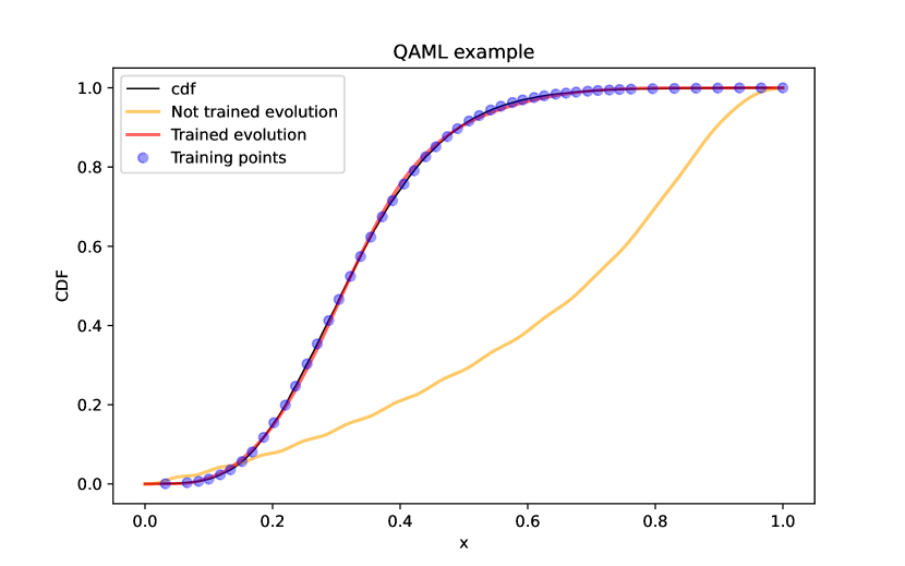
In Fig. 1 an example of this procedure is shown using quantum simulation on classical hardware with the Qibo framework [31, 32, 33, 34, 35]. Starting from a prior toy analytic CDF (black curve), data points are extracted in the interval $x\in[0,1]$. The adiabatic regression model, defined in Sec. II.1 is drawn before training (yellow curve) and after a successful training (red curve). We perform the training of the model by optimizing the set of parameters involved into the scheduling $s(t;\theta)$, defined as the following polynomial of degree $p$:

$$s(t;\theta)=\frac{1}{\eta}\sum_{i=1}^{p}\theta_{i}x^{i},\qquad\text{with}\qquad\eta=\sum_{i=1}^{p}\theta_{i}.$$ (4)

by using the CMA-ES optimizer [36]. In the example shown in (Fig. 1) we set $p=12$, but the polynomial degree can be chosen depending on the complexity of the function one wants to fit. The Eq.(4) is an example of possible choices (one can also choose classical or quantum Neural Network); in particular, every scheduling function such that $s(t=0)=0$ and $s(t=1)=1$ can be used for performing an adiabatic evolution with Qibo. Note that other optimization algorithms may also work, including gradient-based strategies.

Figure 1: Example of initial and final state of the algorithm. The $N_{\rm train}$ blue points are the training set selected from a gaussian mixture sample, whose empirical CDF is represented by the black line. The random initialization of the adiabatic evolution leads to the initial sequence of energies (yellow line). After a training time, the evolution is closer to the training set (red line).

II.3 Probability function from quantum circuits

II.3.1 A circuit for all times

The procedure presented in the previous paragraphs can be interpreted as the evolution product of a series of Hamiltonians corresponding to the adiabatic Hamiltonian configuration at fixed evolution time $\tau=t/T$, discretized according to $\differential\tau$, the time step of the adiabatic evolution. Each of these Hamiltonians can be associated to a local time evolution operator $U(\tau_{n})$ which evolves $\ket{\psi(\tau_{n-1})}$ to $\ket{\psi(\tau_{n})}$. More generally, we can obtain any state $\ket{\psi(\tau_{n})}$ by sequentially applying $n$ operators:

$$\ket{\psi(\tau_{n})}=\prod_{j=0}^{n}U(\tau_{j})\ket{\psi(\tau_{0})}=\mathcal{C}(\tau_{n})\ket{\psi(\tau_{0})}$$ (5)

where we write the product from $n$ to zero to represent the order of application of the operators on the initial quantum state. Any sequence of unitary operator is itself an unitary operator, which we call $\mathcal{C}_{n}=\mathcal{C}(\tau_{n})$ and which evolves the initial state $\ket{\psi(\tau_{0})}$ to any point $\tau_{n}=n\differential\tau$.

In order to compute the state at any value of $t$ outside of the discrete time steps of the adiabatic evolution $\tau$ it is necessary to take the continuous limit. We start by considering one of the intermediate elements of the product:

$$U_{j}=e^{i\text{d}\tau\hat{H}_{j}}\qquad\text{with}\qquad\hat{H}_{j}=\begin{pmatrix}s_{j}&1-s_{j}\\ 1-s_{j}&-s_{j}\end{pmatrix},$$ (6)

where $s_{j}$ is the value of the scheduling at evolution time $\tau_{j}=j\text{d}\tau$. This instantaneous form of the adiabatic hamiltonian operator can be diagonalized as $\hat{D}_{j}$ using a matrix $P_{j}$ such that:

$$\hat{H}_{j}=P_{j}\hat{D}_{j}P_{j}^{-1},$$ (7)

with

$$P_{j}=\Lambda_{j}\begin{pmatrix}1&\frac{s_{j}-\lambda}{1-s_{j}}\\ \frac{\lambda_{j}-s_{j}}{1-s_{j}}&1\end{pmatrix},\qquad\hat{D}_{j}=\begin{pmatrix}\lambda_{j}&0\\ 0&-\lambda_{j}\end{pmatrix},$$ (8)

and $\Lambda_{j}$ the appropriate ($\tau$ dependent) normalization constant. The absolute value of the eigenvalues of the Hamiltonian is $\lambda_{j}=\sqrt{2s_{j}^{2}-2s_{j}+1}$.

We now use this decomposition to write $\mathcal{C}_{n}$ in terms of the diagonal form of the Hamiltonian:

$$\mathcal{C}_{n}=\prod_{j=0}^{n}P_{j}e^{i\differential\tau\hat{D}_{j}}P_{j}^{-1}.$$ (9)

If we now take the limit $\differential\tau\to 0$, we have that $\hat{H}_{j}\to\hat{H}_{j-1}$ and thus $P_{j}\to P_{j-1}$. Thus adjacent elements in the sequence tend to the identity: $P_{j}^{-1}P_{j-1}\to I$. On this way, the Eq. (9) simplifies to:

$$\mathcal{C}_{n}=P_{n}\exp{i\sum_{j=0}^{n}\hat{D}_{j}\differential\tau}P_{0}^{-1}.$$ (10)

Furthermore, in the limit of $\differential\tau\to 0$ the sum in the above equation becomes an integration in $\differential\tau$ with extremes $\tau=0$ and $\tau=\tau_{n}$. With the final expression for $\mathcal{C}$ evaluated at any time $t$ being:

$$\mathcal{C}(t)=P_{t}\exp{i\displaystyle\int_{0}^{t/T}\hat{D}_{j}\differential\tau}P_{0}^{-1},$$ (11)

where we now indicate with $P_{t}$ and $P_{0}$ the diagonalization matrices corresponding respectively to the last and the first evolution operators we must apply to $H_{0}$’s ground state in order to obtain the evolved state at time $t$.

II.3.2 Circuit representation

Let us implement the unitary operator $\mathcal{C}(t)$, which allows us to prepare a state in the ground state of $H_{0}$ at $t=0$ and evolve it to any $t$, using a gate decomposition which is useful for calculating the derivatives of the circuit with respect to its variational parameters. To that end we write $\mathcal{C}(t)$ in terms of rotations $R_{y}$, $R_{z}$. Since any unitary operator $U\in SU(2)$ can be written as a combination of three rotations [37] we choose:

$$\mathcal{U}\equiv R_{z}(\phi)R_{x}(\theta)R_{z}(\psi),$$ (12)

where the three angles $(\phi,\theta,\psi)$ can be computed as function of the matrix element of the operator $\mathcal{C}$:

$$\begin{cases}\phi=\pi/2-\text{arg}(c_{01})-\text{arg}(c_{00})\\ \theta=-2\arccos(|c_{00}|)\\ \psi=\text{arg}(c_{01})-\pi/2-\text{arg}(c_{00}).\end{cases}$$ (13)

The matrix elements $c_{00}$ and $c_{01}$ depend on the values of the scheduling $s$ and the eigenvalues ($\lambda$) of the Hamiltonian evaluated at a time $t$:

$$c_{0j}=\frac{1-s}{s\sqrt{\lambda(\lambda-s)}} \left\{\cos{I}\left(1+(-1)^{j}\frac{\lambda-s}{1-s}\right)\right.$$

$$+\left.i\sin{I}\left(1-(-1)^{j}\frac{\lambda-s}{1-s}\right)\right\},$$ (14)

with $I=\displaystyle\int_{0}^{t}\lambda(\tau)\differential\tau$, $s=s(t)$ and $\lambda=\lambda(t)$.

Note that the construction of the circuit is completely independent of the choice of scheduling function $s(t)$.

II.3.3 From the CDF to the PDF

The circuit representation of the operator $\mathcal{C}(t)$ allows us to reconstruct our original target function $f(x)$ by applying the circuit to a state prepared at $\ket{\psi(0)}$ and then measuring the desired observable, which in our case is a non-interacting Pauli $\hat{Z}$. Since with qibo we translate all the operations into a circuit representation, the expectation value of $\hat{Z}$ is evaluated by executing the circuit $N_{\rm shots}$ times and then by calculating the probability of occurrence of the state $\ket{0}$. This expectation value is then used as estimation of the target function $f(x)$.

As previously said, our example case has been that in which the target function $f(x)$ correspond to the empirical CDF of some arbitrary distribution.

By imposing monotonicity and pinning the initial and final points we ensure that its first derivative correspond to the PDF of the same distribution.

For a 1D distribution we have then:

$$\frac{\differential f(t)}{\differential t}=\frac{\differential}{\differential t}\braket{\psi_{0}}{\mathcal{C}(t)^{\dagger}\hat{Z}\mathcal{C}(t)}{\psi_{0}}.$$ (15)

In the context of quantum computing, we can take advantage of what is usually known as Parameter Shift Rule (PSR) [26, 38] which allows us to take the derivative of an observable (such as Eq. (15)) by simply evaluating the circuit and shifting the parameters with respect to which we are taking the derivative. We are using specifically choice presented in Ref. [26] for circuits based on rotations. Note that in this case we have limited ourselves to gates in which the parameter appears only once, but more complicated forms can also be utilized [39].

With this we arrive to the final formula of the PDF in terms of the original circuit:

$$\text{PDF}(t)=\text{PSR}\left[\braket{\psi_{0}}{\mathcal{C}(t)^{\dagger}\hat{Z}\mathcal{C}(t)}{\psi_{0}}\right].$$ (16)

In the following we “closure test” these techniques by drawing samples from a known distribution, building the circuit and reconstructing the original probability function.

III Validation

III.1 Sampling known distributions

Figure 2: Top row: comparisons between the true CDF and the result of training an adiabatic hamiltonian to follow the CDF from the sampled distribution. The exact CDF is represented by a discontinuous black line while the simulated circuit results are represented by a blue (realistic) and red (ideal) continuous lines. In grey an arbitrary binning of the data that has been used to train the circuit. Bottom row: comparison between the original PDF and the result of the derivative of the trained circuit. Once again the true result is represented by a discontinuous black, the data histogram is shown in grey and the exact simulation of the circuit is represented as a red continuous line. As regarding the realistic simulations, we show two different continuous lines, corresponding to different values of shots used for evaluating the expectation value of the target observable. In particular, we show in orange and blue the results obtained executing the circuit respectively $N_{\rm shots}=2\cdot 10^{4}$ and $N_{\rm shots}=2\cdot 10^{5}$ times. All af these results are shown in the form of a ratio between the target true law and the QML estimations in the lowest part of the figures. While representing the PDFs, only one realistic simulation is drawn ($N_{\rm shots}=2\cdot 10^{5}$). All the realistic simulations curves are represented together with a $1\sigma$ confidence belt calculated using $N_{\rm runs}=20$ experiments.

Figure 3: The top row shows the CDF of the three HEP samples. In each figure, the histogram of the data is shown in gray, the CDF obtained by exact state vector simulation is shown in red, and the same result is shown in blue but considering realistic circuits executed $N_{\rm shots}=2\cdot 10^{5}$ times. The bottom row shows the PDF of three sampled HEP distributions. They are divided into two parts: above, in grey the histogram of the sample used to perform the fit in which we impose $N_{\rm mbins}=34$ (this is the lowest number of bins thanks to which we can represent well the right side of the $s$ and $t$ distributions), and the curves representing the PDF of the sample: in red the law extracted via QML using exact state vector simulation on $N_{\rm times}=500$ times equally distributed between $0$ and $1$, and in blue the law obtained with the same approach but simulating a realistic circuit in which we calculate the expected value of the target observable by executing the circuit $N_{\rm shots}=2\cdot 10^{5}$ times. Below, we show the ratio between the histogram values of the PDF and our simulated results: the red line corresponds to the exact simulation, the orange and blue lines respectively correspond to realistic simulations in which we set $N_{\rm shots}=2\cdot 10^{4}$ and $N_{\rm shots}=2\cdot 10^{5}$. All the realistic simulations curves are represented together with a $1\sigma$ confidence belt calculated using $N_{\rm runs}=20$ experiments.

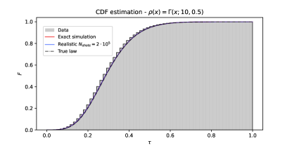
In order to validate and test the procedure, we select a number of known prior distributions. For each cases, we generate a representative sample of dimension $N_{\rm sample}$ and fit the resulting empirical CDF using the approach described in Sec. II.1. We can then derive the PDF and compare results to the prior distribution. We repeat this exercise twice for every example by using quantum simulation on classical hardware with exact state-vector representation and with shots measurements.

In these examples the algorithm is set to stop once a given $J_{\rm cut}$ threshold of target precision is reached and the domain of the target variable is rescaled to be between $0$ and $1$ so that the interpretation of the observable as a CDF is direct. This is of course just a choice and the same techniques could be used to train functions defined in any arbitrary domain. In all cases the adiabatic evolution is run for $T=50$s and with a time-step $\differential t=0.1$. We define the scheduling function a as a polynomial with $p$ parameters following the ansatz in Eq. 4.

We start by drawing samples from the Gamma distribution, defined as

$$\rho(x;\alpha,\beta)=\frac{\beta x^{\alpha-1}e^{\beta x}}{\Gamma(\alpha)},$$ (17)

with $\alpha=10$ and $\beta=0.5$. We draw $N_{\rm samples}=5\cdot 10^{4}$ points and train the scheduling function until a target precision of $J_{\rm cut}=10^{-5}$ is reached.

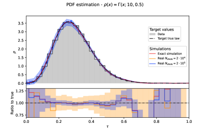
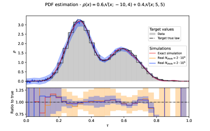
The results of the training can be seen in the first row and left column of Fig. 2 where we plot the true CDF together with both the exact and realistic simulation and an histogram with the data used for the training. In the second row and left column of Fig. 2 we show the PDF obtained by taking the derivative of the circuit and compare to the original distribution from which the original points were sampled from. We also show the effect of modifying the number of shots (i.e., the number of times we measure the qubit before accepting the results). In both these figures we show the exact results (i.e., following the formula from Eq. (17)) in black and the exact simulation using state vectors in blue. In red instead, we show the results considering realistic circuits (where the collapse of the states is simulated by a classical sampling from the state vector). The error bands plots in the second row of Fig. 2 are computed by taking all realizations of the measurement and computing the standard deviation for each point in $t$. We plot two different choices ($N_{\rm shots}=\{2\cdot 10^{4},2\cdot 10^{5}\}$) for the number of shots in order to show how the result improves with the increased statistics.

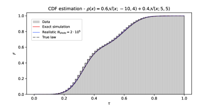
In order to validate with a more complicated example we also sample from a Gaussian mixture defined as:

$$\rho(x;\vec{\mu},\vec{\sigma})=0.6\mathcal{N}(x;\mu_{1},\sigma_{1})+0.4\mathcal{N}(x;\mu_{2},\sigma_{2}),$$ (18)

with $\vec{\mu}=(-10,5)$ and $\vec{\sigma}=(5,5)$. From this distribution we take $N_{\rm sample}=5\cdot 10^{5}$ points to generate the training sample.

In the right column of Fig. 2 we repeat the same study. The fit performs slightly worse due to the more complicated nature of the target function, the hardware already limits the level of precision that can be achieved.

In both these cases we train the adiabatic evolution as implemented in qibo [35, 34, 40, 41]. While the parameter optimization is made by means of a CMA-ES [36] genetic algorithm. The final Hamiltonian is then transformed into a circuit as explained in section II.3.1.

In order to produce the plots we perform two estimations. During simulation we can apply the circuit exactly to the ground state of $H_{0}$ at every point in $t$ such that we can show an “exact” (although ideal and nonphysical) situation. The more realistic result instead is estimated by running the same circuit several time simulating the actual randomness of a quantum device. This is implemented in Qibo through the method AbstractHamiltonian.expectation_from_samples. which can perform a realistic simulation.

When calculating the derivatives of the rotation angles with respect to $t$, which we call $\partial_{t}\theta$, some critical points of instability are found. For those $t$’s the value of the derivative of the angle increase exponentially; in the case of the exact simulation, the value of the PSR for the same points is very close to zero and this balances the divergence of $\partial_{t}\theta$. On contrary, when dealing with the realistic simulations, the PSR value is estimated through the mean of $N_{\rm shots}$ realizations and it can be possible that it is not close to zero enough to balance the high values of the angles. In order to avoid a numerical instability for $t_{j}$ (which leads to a few high peaks of the estimated PDFs), we smooth the realistic function by removing the outlier using the values registered for the neighbours of $t_{j}$.

III.2 Density estimation using LHC data sampled from the Style-qGAN model

While in the previous case we were training the circuit using a sampling from a known distribution, we know move to the more complex case of learning an unknown distribution. We consider the particle physics process involving top and anti-top quark pair production ($pp\to t\bar{t}$). While one could train directly by using the output of an event generator in our test case the data sampling is obtained from a separated circuit by using a style-based quantum GAN (Style-qGAN) [42].

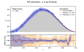
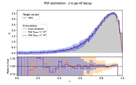
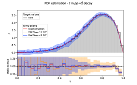
The Style-qGAN has been trained with $10^{5}$ events for $pp\to t\bar{t}$ production at a center of mass of $\sqrt{s}=13$ TeV for the LHC configuration. For simplicity we limit the simulation at Leading Order in the strong coupling. The fit is done by training the model to the distributions of the rapidity $y$ and the logarithms of the Mandelstam variables $-\log{(-t)}$ and $-\log{s}$.

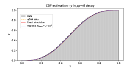
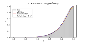
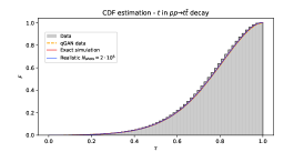
In Fig. 3 we show the results for the training of the circuit (the CDF on the top row) and its derivative (the PDF on the bottom row), following the same conventions as in the previous section.

In Table 1 we summarize the obtained results for all examples tested in this section. For each model we describe the final configuration and quality of the obtained model by calculating the following test statistics:

$$\chi^{2}=\sum_{i=0}^{N_{train}}\frac{(\hat{y}_{i}-y_{i})^{2}}{y_{i}},$$ (19)

where $\hat{y}_{i}$ correspond to the estimated values and $y_{i}$ the target ones. and the target ones.

Fit function	$N_{\rm sample}$	$p$	$J_{f}$	$N_{\rm ratio}$	$\chi^{2}$
Gamma	$5\cdot 10^{4}$	$25$	$2.9\cdot 10^{-6}$	$31$	$2.2\cdot 10^{-4}$
Gaussian mix	$2\cdot 10^{5}$	$30$	$2.75\cdot 10^{-5}$	$31$	$4.39\cdot 10^{-3}$
$t$	$5\cdot 10^{4}$	$20$	$2.1\cdot 10^{-6}$	$34$	$3.4\cdot 10^{-4}$
$s$	$5\cdot 10^{4}$	$20$	$7.9\cdot 10^{-6}$	$34$	$1.20\cdot 10^{-3}$
$y$	$5\cdot 10^{4}$	$8$	$3.7\cdot 10^{-6}$	$34$	$1.45\cdot 10^{-3}$

Table 1: Summary. $N_{\rm shots}=5\cdot 10^{4}$.

In summary, the achieve level of quality is satisfactory for all tested distributions. We also observe that $N_{\rm shots}=2\cdot 10^{5}$ shots provides sufficient statistics to achieve a precision in the range of 4-10% (see ratio plots in the bottom part of Fig. 2 and Fig. 3). The precision range quoted is calculated by taking the measurements which are farthest from the central value in order to give an idea of the worst-case-scenario of the estimation. The range doesn’t account for the regions in which the distribution is very small and where outliers can generate big relative errors.

IV Hardware

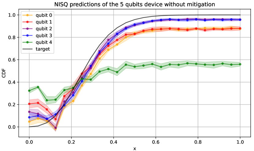
We use a 5-qubits superconducting chip hosted in the Quantum Research Centre (QRC) of the Technology Innovation Institute (TII) for testing the algorithm on the hardware. We calculate the predictions for the values of the CDF using the best parameters obtained through the training with the shot-noise simulation whose results are presented in Tab. 1. We take into account the Gamma distribution defined in Eq. (17) and we do not apply error mitigation techniques to the hardware, in order to explore the potentialities of the bare chips.

We consider $N_{\rm data}=25$ points equally distributed in the target range $[0,1]$ and for each of these we perform $N_{\rm runs}=10$ predictions executing $N_{\rm shots}=1000$ times the circuit on the quantum hardware. Using these data, we calculate the final predictors and their uncertaintes as mean and standard deviation over the $N_{\rm runs}$ results. We also calculate as test statistics $K$ the average ratio between predictions and labels. We repeat this procedure for each of the five qubit of the device. The results are shown in Fig. 4 and are in agreement with Tab. 2, where we report the assignment fidelities [43] of the qubits.

Qubit ID	assignment fidelity	$K$
$0$	$0.926$	$3.0$
$1$	$0.886$	$10.2$
$2$	$0.953$	$6.8$
$3$	$0.952$	$4.8$
$4$	$0.707$	$15.5$

Table 2: Calculated average ratios $\hat{y}/y$ in comparison with the registered assignment fidelities of the five chips.

In this part of the work we aim to study how the CDF predictions deteriorate if performed on hardware and what is the impact of detuning the qubits’ fidelities.

The quantum hardware control is performed using Qibolab [40] and the qubits are characterized and calibrated executing the Qibocal’s routines [44, 41].

Figure 4: $N_{\rm runs}=10$ predictions are performed for $N_{\rm data}=25$ points in the target range $[0,1]$ using each qubit of a 5-qubits device hosted in the QRC.

V Conclusion

In this work we presented a methodology for the determination of probability density functions using adiabatic quantum computing. We first define a mechanism to use adiabatic evolution as a regression model for the fit of empirical cumulative density function which are represented by the Trotterization of the adiabatic Hamiltonian in terms of a quantum circuit. The PDF is then calculated by applying the Parameter Shift Rule to the obtained circuit. This methods allows the usage for training and inference of quantum devices designed for annealing and circuit-based technologies. The numerical results obtained and presented in Sec. III show successful applications of the methodology for predefined PDFs and empirical distributions obtained from high-energy particle physics observables. The results obtained on superconducting devices and presented in Sec. IV are promising: with a good calibration of the chips, CDFs can be fitted even without mitigation techniques.

All numerical results have been obtained with Qibo framework , and are publicly available in . Further possible developments include the generalization of this method for the simultaneous determination of multi-dimensional PDF distributions, the deployment of the full training procedure on quantum devices and the possibility to use quantum annealing for the optimization of the regressing model parameters. A direct extension of the method presented in this manuscript can be applied to multi-dimensional PDFs depending on Identically Indipendend Distributed (IID) variables. In this case the presented algorithm can be indipendently executed on a number of qubits equal to the number of variables.