Lipschitz complexity

Abstract.

Quantum complexity theory is concerned with the amount of elementary quantum resources needed to build a quantum system or a quantum operation. The fundamental question in quantum complexity is to define and quantify suitable complexity measures. This non-trivial question has attracted the attention of quantum information scientists, computer scientists, and high energy physicists alike. In this paper, we combine the approach in [LBK⁺22] and well-established tools from noncommutative geometry [Con90, Rie99, CS03] to propose a unified framework for resource-dependent complexity measures of general quantum channels, also known as Lipschitz complexity. This framework is suitable to study the complexity of both open and closed quantum systems. The central class of examples in this paper is the so-called Wasserstein complexity introduced in [LBK⁺22, PMTL21]. We use geometric methods to provide upper and lower bounds on this class of complexity measures [Nie06, NDGD06a, NDGD06b]. Finally, we study the Lipschitz complexity of random quantum circuits and dynamics of open quantum systems in finite dimensional setting. In particular, we show that generically the complexity grows linearly in time before the return time. This is the same qualitative behavior conjecture by Brown and Susskind [BS18, BS19]. We also provide an infinite dimensional example where linear growth does not hold.

1. Introduction

Quantum complexity is a fundamental concept in quantum information and quantum computation theory. It is a generalization of classical computational complexity and characterizes the inherent difficulty of various quantum information tasks. Compared with classical complexity, quantum complexity is much more difficult to quantify and measure. By now, there are numerous inequivalent quantum complexity measures [OT08, RW05, Wat03, FR99, DP85, Kla00, BT09, BV97, BASTS08, BGS95, BS07, HKH⁺22]. On one hand, quantum information specialists primarily focus on the quantum circuit complexity, which emphasizes on the number of elementary gates required to simulate a complex unitary transformation [Nie06, NDGD06a, NDGD06b, LBK⁺22, HFK⁺22, FGHZ05]. On the other hand, high energy physicists have adapted the notion of complexity to systems with infinite degrees of freedom [JM17, HR23, BS18, BS19, Ali15] and to chaotic quantum systems [PCA⁺19, DS21, AAS22, RSGSS21, RSGSS22, BNNS22, BCNP23, BNNS23].

From information theoretic perspective, any computational task can be characterized as an information channel. This is certainly the case in classical computers, where different logical and memory components communicate with each other and accomplish complex computational tasks in coordination. Therefore, when studying quantum complexity measures, it is reasonable to focus on the complexity of general quantum channels. In addition, any reasonable complexity measure must take into consideration the amount of available computational resources. Plainly, if given infinite resources (e.g. all possible unitary gates), then any computational task would have low complexity. The resources for quantum computation typically come in the form of a set of simple unitary gates or a set of simple infinitesimal generators that can drive the time evolution of a quantum system. When considering time evolution in this paper, we do not restrict to the unitary evolution of closed quantum systems. Since any realistic quantum system must interact with the environment, it is more natural to consider time evolution of open quantum systems.

With these considerations in mind and following the axiomatic approach in [LBK⁺22], we propose a set of general axioms that any resource-dependent complexity measure of quantum channels should satisfy. The main novelty of our axiomatic framework is a combination of complexity theory [LBK⁺22] and well-established operator algebraic tools [Con90, Rie99, CS03, GJL20a, CM17, CM20, Wir18]. Our proposed axioms do not require the resources to have a particular form. Therefore it provides a unified framework that can be applied to unitary gate sets and infinitesmial generators. In addition, the axioms consider general quantum channels and hence are suitable to study the complexity of time evolution of both closed and open systems. Finally, our axioms can also be used to study the dynamics of complexity measures.

The main example of complexity measure in this paper is the so-called Wasserstein complexity [LBK⁺22, PMTL21]. This is a complexity measure based on a noncommutative analog of the classical Lipschitz norm [CM17, CM20, Wir18, GJL20a]. It is well-known that the Wasserstein 1-norm is dual to the Lipschitz norm. Our definition of the Lipschitz norm is based on noncommutative geometry [Con90, Rie99]. And it is a generalization of the existing notion [PMTL21]. Since the noncommutative Lipschitz norm (or dually the Wasserstein norm) studies the noncommutative differential structure on the state space (or dually the observables), the Lipschitz complexity naturally adopts the geometric perspective on quantum complexity first introduced by Nielsen [Nie06, NDGD06a, NDGD06b]. Depending on the applications, we will introduce several different notions of noncommutative Lipschitz norms. Each definition leads to a different quantum complexity measure satisfying the proposed axioms.

One of the central problems in quantum complexity theory is to provide tight estimates on the complexity measures. Typically a lower bound on the complexity is more informative for the purpose of classification. In this paper, we will provide various upper and lower bounds for the Lipschitz complexity. The upper bound estimates are typically derived from geometric arguments similar to the original Nielsen’s estimates [Nie06, NDGD06a, NDGD06b], while the lower bound estimate relies on the noncommutative return time estimate and a notion of size of the Lipschitz space. In the noncommutative setting, it is simply the Lipschitz complexity of the conditional expectation onto the fixed point of a quantum channel. Since the conditional expectation itself is a special type of quantum channel, we will have better control over its Lipschitz complexity. And by relating the Lipschitz complexity of general channels to that of the conditional expectations, we will be able to bound the complexity of general channeles.

As mentioned above, our approach to quantum complexity is suitable to study the evolution of complexity with time. Given a time-dependent quantum channel (e.g. a quantum Markov semigroup), we can study the time evolution of its Lipschitz complexity. This is closely related to the Brown-Susskind conjecture [BS18, BS19, HFK⁺22]. The conjecture states that for a generic quantum circuit, its circuit complexity grows linearly with time (measured in terms of the depth of the circuit and the number of gates used in the circuit) and the complexity saturates at a value that is exponential in the system size [BS18, BS19]. This conjecture was proved for random quantum circuits [HFK⁺22]. We will show that, for a quantum Markov semigroup, the Lipschitz complexity first grows linearly in time and then saturates at a maximal value. In addition, the time scale to saturate the maximum can be calculated by the return time of the quantum Markov semigroup. Qualitatively, this is the same behavior as conjectured by Brown and Susskind [BS18, BS19]. Our result suggests that for any generic time-dependent quantum channel (not necessarily given by a quantum circuit), its complexity should have the qualitative behavior of the Brown-Susskind type. Finally, we remark here that this linear growth behavior occurs only in finite dimension, and we give a counterexample in infinite dimension setting showing linear growth fails.

2. Axioms of Lipschitz complexity measures of quantum channels

In this section, we present the axioms of resource-dependent complexity measures of quantum channels. We state the axioms for finite-dimensional quantum systems. But it is possible to generalize these axioms to any finite von Neumann algebras as in [GJL20a].

Let $\mathcal{H}$ be a Hilbert space and let $\mathbb{B}(\mathcal{H})$ be the bounded operators on $\mathcal{H}$. Suppose $\mathcal{N}\subset\mathbb{B}(\mathcal{H})$ is a finite dimensional von Neumann algebra. Denote the canonical trace on $\mathcal{N}$ by $\operatorname{tr}$. Recall that a quantum channel is a normal, trace-preserving, completely positive map:

$$\Phi:\mathcal{N}_{*}\to\mathcal{N}_{*},$$

where $\mathcal{N}_{*}\cong L_{1}(\mathcal{N})$ is the space of normal density functionals.

The dual map $\Phi^{*}:\mathcal{N}\to\mathcal{N}$ defined via $\operatorname{tr}(\Phi^{*}(\rho)x)=\operatorname{tr}(\rho\Phi(x))$ for any $\rho\in L_{1}(\mathcal{N}),x\in\mathcal{N}$, is a normal unital completely positive map.

As mentioned in the introduction, typically the resources for quantum computations can be characterized by a set of simple unitaries or a set of simple infinitesimal generators. Heuristically, the goal of resource-dependent complexity measure is to quantify the amount of resources needed to construct a given quantum channel. Mathematically, motivated by [LBK⁺22, HR23, PMTL21] our goal is to find an appropriate complexity function $C$ defined on quantum channels

$$C:CP(\mathcal{N})\to\mathbb{R}_{\geq 0},$$

where $CP(\mathcal{N})$ is the set of all the quantum channels on $\mathcal{N}$, such that it satisfies some of the following axioms:

Axioms 1.

1. $C(\Phi)=0$ if and only if $\Phi=\rm{id}$.

2. (subadditivity under concatenation) $C(\Phi\Psi)\leq C(\Phi)+C(\Psi)$.

3. (Convexity) For any probability distribution $\{p_{i}\}_{i\in I}$ and any channels $\{\Phi_{i}\}_{i\in I}$, we have

   (2.1) $$C(\sum_{i\in I}p_{i}\Phi_{i})\leq\sum_{i\in I}p_{i}C(\Phi_{i}).$$

4. (Tensor additivity) For finitely many channels $\{\Phi_{i}\}_{1\leq i\leq m}$, we have

   (2.2) $$C(\bigotimes_{i=1}^{m}\Phi_{i})=\sum_{i=1}^{m}C(\Phi_{i}).$$

5. (Normalization) $C(\Phi)\leq O(\log d)$, where $d$ is the dimension of the underlying Hilbert space, if $C(\Phi)<\infty$.

The physical intuition behind these axioms is clear:

1. Trivial identity channel should have no complexity.

2. The subadditivity clause axiomatizes the fact that, when building complex channels from simpler ones, the overall complexity cannot be larger than the sum of the individual complexities. In other words, one cannot create complexity out of thin air. On the other hand, a decrease in complexity should be allowed.

3. The convexity clause is the fact that statistical ensemble of channels cannot create more complexity than the statistical mean of the individual complexities.

4. Tensor additivity clause is the fact that the complexity of building independent quantum channels should be the same as the sum of complexity of building each channel.

5. Normalization clause gives us a limit based on the number of qubits we have.

To propose such a complexity function, motivated by [LBK⁺22], we will introduce a Lipschitz norm, which is widely used in [Con90, Rie99, CS03, GJL20a, CM17, CM20, Wir18] and fruitful theories were built there.

Recall that a derivation triple is given by $(\mathcal{A},D,\mathcal{H})$, where $D:\mathcal{A}\to\mathcal{M}$ where $\mathcal{M}$ is a larger von Neumann algebra, is a non-commutative differential operator and $\mathcal{A}\subset\mathbb{B}(\mathcal{H})$ is a $*$-subalgebra such that $\|D(a)\|<\infty$ for any $a\in\mathcal{A}$. Typically, $D(x)=[d,x]$ where $d$ is a self-adjoint operator.

2.1. Single-system Lipschitz complexity

We are ready to introduce the resource-dependent complexity function for single system. The resources are nothing but a set of operators. To be specific, suppose $S\subset\mathcal{N}$ is a subset, the induced Lipschitz (semi-)norm is defined by

(2.3) $$|||f|||_{S}:=\sup_{s\in S}\|[s,f]\|_{\infty},\ f\in\mathcal{N}.$$

Definition 2.1.

For a quantum channel $\Phi:\mathcal{N}_{*}\to\mathcal{N}_{*}$, the complexity is defined as

(2.4) $$C_{S}(\Phi):=\|\Phi^{*}-\rm{id}:(\mathcal{N},|||\cdot|||_{S})\to\mathbb{B}(\mathcal{H})\|.$$

We denote the above norm by $\|\Phi^{*}-\rm{id}\|_{Lip\to\infty}$ for simplicity in the following proofs.

Note that $|||f|||_{S}$ is a semi-norm. In order to make it a true norm, we need to restrict on a subspace. To this end, we define the space of mean 0 Lipschitz space $\mathcal{A}$ as the quotient space

$$\mathcal{A}:=\mathcal{N}/\{f\in\mathcal{N}:|||f|||_{S}=0\}.$$

Recall the commutant of $S$ is given by

(2.5) $$S^{\prime}=\{f\in\mathcal{N}:[s,f]=0,\ \forall s\in S\}.$$

Denote the trace-preserving conditional expectation onto $S^{\prime}$ as $E_{S^{\prime}}:\mathcal{N}\to S^{\prime}$. Then it is easy to see that

(2.6) $$\mathcal{A}\cong\{f\in\mathcal{N}:E_{S^{\prime}}(f)=0\}.$$

In other word, $\mathcal{A}$ is orthogonal to the algebra $S^{\prime}$. The definition of complexity for single system is given as follows: The elementary properties are summarized in the following lemma:

Lemma 2.2.

1. $C_{S}(\Phi)=0$ if and only if $\Phi=\rm{id}$.

2. $C_{S}(\Phi\Psi)\leq C_{S}(\Phi)+C_{S}(\Psi)$ for any quantum channels $\Phi,\Psi$.

3. For any probability distribution $\{p_{i}\}_{i\in I}$ and any channels $\{\Phi_{i}\}_{i\in I}$, we have

   (2.7) $$C_{S}(\sum_{i\in I}p_{i}\Phi_{i})\leq\sum_{i\in I}p_{i}C_{S}(\Phi_{i}).$$

4. $C_{S}(\Phi)\leq C_{S}(E_{S^{\prime}})\|\Phi^{*}-\rm{id}:\mathcal{N}\to\mathcal{N}\|$.

Proof.

Property $(1)$ follows from the faithfulness of the norm and property $(3)$ follows from the triangle inequality of norm. We only need to show $(2),(4)$. To show $(2)$, note that

$$\begin{split}C_{S}(\Phi\circ\Psi)&=||\Psi^{*}(\Phi^{*}-id)+\Psi^{*}-id||_{Lip\to\infty}\leq||\Psi^{*}||_{\infty\rightarrow\infty}||\Phi^{*}-id||_{Lip\rightarrow\infty}+||\Psi^{*}-id||_{Lip\rightarrow\infty}\\ &\leq C_{S}(\Psi)+C_{S}(\Phi)\end{split}$$

where for the first inequality, we use the following diagram and submultiplicativity of norms:

and for the last inequality, we used the fact that a unital completely positive map $\Psi^{*}$ satisfies $||\Psi^{*}||_{\infty\to\infty}\leq||\Psi^{*}||_{cb}\leq 1$. To show $(4)$, we use the following diagram and submultiplicativity of norms:

$$||\Phi^{*}-id||_{Lip\rightarrow\infty} \leq||id||_{Lip\rightarrow\infty}||\Phi^{*}-id||_{\infty\rightarrow\infty}$$

$$=||id-E_{S^{\prime}}^{*}||_{Lip\rightarrow\infty}||\Phi^{*}-id||_{\infty\rightarrow\infty}=C_{S}(E_{S^{\prime}})||\Phi^{*}-id||_{\infty\rightarrow\infty},$$

where for the second last equality, we used the fact that for any $x\in\mathcal{A},E_{S^{\prime}}(x)=0$. ∎

The effects of the environment on quantum systems are usually taken into consideration, which means we need to allow our system to couple with an additional system. Next we define a complete version of the complexity, or correlation assisted version.

Given a resource set $S\subset\mathcal{N}$, the $n$-th amplification of the Lipschitz norm is defined as

(2.8) $$|||f|||^{n}_{S}=\sup_{s\in S}\|[I_{n}\otimes s,f]\|,f\in\mathbb{M}_{n}(\mathcal{A}).$$

This enables us to define complete complexity:

Definition 2.3.

The complete(correlation-assisted) complexity of a quantum channel $\Phi$ is defined by

(2.9) $$C_{S}^{cb}(\Phi):=\sup_{n\geq 1}\|\rm{id}_{n}\otimes(\Phi^{*}-\rm{id}):(\mathbb{M}_{n}(\mathcal{A}),|||\cdot|||^{n}_{S})\to\mathbb{M}_{n}(\mathbb{B}(\mathcal{H}))\|.$$

All the above elementary properties hold true by the same argument. We summarize the results as follows:

Lemma 2.4.

1. $C_{S}^{cb}(\Phi)=0$ if and only if $\Phi=\rm{id}$.

2. $C_{S}^{cb}(\Phi\Psi)\leq C_{S}^{cb}(\Phi)+C_{S}^{cb}(\Psi)$ for any quantum channels $\Phi,\Psi$.

3. For any probability distribution $\{p_{i}\}_{i\in I}$ and any channels $\{\Phi_{i}\}_{i\in I}$, we have

   (2.10) $$C_{S}^{cb}(\sum_{i\in I}p_{i}\Phi_{i})\leq\sum_{i\in I}p_{i}C_{S}^{cb}(\Phi_{i}).$$

4. $C_{S}^{cb}(\Phi)\leq C_{S}^{cb}(E_{S^{\prime}})\|\Phi-\rm{id}\|_{\diamond}$.

Now we list some useful techniques on bounding the complexity of quantum channels, which will be used throughout the paper.

Mixing time and return time trick

Denote $\mathcal{N}_{fix}=S^{\prime}$ and we assume it is a von Neumann subalgebra and denote $E_{fix}$ as the tracial conditional expectation onto $\mathcal{N}_{fix}$.

For any quantum channel $\Phi$ with $\Phi^{*}E_{fix}=E_{fix}$, we can define the mixing time of $\Phi$ as follows: for $\varepsilon>0$,

(2.11) $$t_{mix}(\varepsilon,\Phi):=\inf\{n\geq 1:\|\Phi^{n*}-E_{fix}:\mathcal{N}\to\mathcal{N}\|=\|\Phi^{n}-E_{fix}:L_{1}(\mathcal{N})\to L_{1}(\mathcal{N})\|\leq\varepsilon\}.$$

For the complete version, we denote

(2.12) $$t_{mix}^{cb}(\varepsilon,\Phi):=\inf\{n\geq 1:\|\Phi^{n*}-E_{fix}\|_{cb}=\|\Phi^{n}-E_{fix}\|_{\diamond}\leq\varepsilon\}.$$

Similarly, we can also define the return time of the quantum channel. For $\varepsilon>0$,

(2.13) $$t_{ret}(\varepsilon,\Phi):=\inf\{n\geq 1:(1-\varepsilon)E_{fix}\leq_{cp}\Phi^{n*}\leq_{cp}(1+\varepsilon)E_{fix}\}.$$

And the definition of the complete version $t^{cb}_{ret}(\varepsilon,\Phi)$ is similar. Note that if $\Phi$ is symmetric, the above definition coincides with the definition in [GJLL22]. It is directly to see that

(2.14) $$t_{mix}^{cb}(\varepsilon,\Phi)\leq t^{cb}_{ret}(\varepsilon,\Phi)$$

since $\|\cdot\|_{cb}\leq\|\cdot\|_{1\to\infty,cb}$.

Lemma 2.5.

For any channel $\Phi$ with $\Phi^{*}E_{fix}=E_{fix}$, we assume that for some $\varepsilon>0$, the (complete) mixing time is finite. Then we have

(2.15) $$(1-\varepsilon)C^{(cb)}_{S}(E_{fix})\leq t^{(cb)}_{mix}(\varepsilon,\Phi)C^{(cb)}_{S}(\Phi)\leq t^{(cb)}_{ret}(\varepsilon,\Phi)C^{(cb)}_{S}(\Phi).$$

Proof.

We only show $(1-\varepsilon)C_{S}(E_{fix})\leq t_{mix}(\varepsilon,\Phi)C_{S}(\Phi)$ and the correlation-assisted version holds true by just replacing every channel by its amplification. Without loss of generality, we assume $k=t_{mix}(\varepsilon,\Phi)<\infty$, then we have

(2.16) $$\|(\Phi^{*})^{k}-E_{fix}\|_{\infty\to\infty}\leq\varepsilon.$$

Calculating $C_{S}(E_{fix})$, we have

$$C_{S}(E_{fix}) =\|E_{fix}-id:(\mathcal{A},|||\cdot|||_{S})\to L_{\infty}(\mathcal{N})\|$$

$$=\|E_{fix}-(\Phi^{*})^{k}+(\Phi^{*})^{k}-id:(\mathcal{A},|||\cdot|||_{S})\to L_{\infty}(\mathcal{N})\|$$

$$\leq C_{S}(\Phi^{k})+\|E_{fix}-(\Phi^{*})^{k}:(\mathcal{A},|||\cdot|||_{S})\to L_{\infty}(\mathcal{N})\|.$$

Recall that $\Phi^{*}E_{fix}=E_{fix}$ we have $(\Phi^{*})^{k}E_{fix}=E_{fix}$ thus

(2.17) $$E_{fix}-(\Phi^{*})^{k}=(E_{fix}-(\Phi^{*})^{k})(id-E_{fix}).$$

Using the following diagram

we have

$$\|E_{fix}-(\Phi^{*})^{k}:(\mathcal{A},|||\cdot|||_{S})\to L_{\infty}(\mathbb{M}_{d})\| \leq C_{S}(E_{fix})\|(\Phi^{*})^{k}-E_{fix}\|_{\infty\to\infty}$$

$$\leq\varepsilon C_{S}(E_{fix}).$$

In summary, we showed that

$$C_{S}(E_{fix})\leq\varepsilon C_{S}(E_{fix})+C_{S}(\Phi^{k})\leq\varepsilon C_{S}(E_{fix})+kC_{S}(\Phi),$$

which implies $(1-\varepsilon)C_{S}(E_{fix})\leq t(\varepsilon,\Phi)C_{S}(\Phi)$. ∎

The next lemma makes use of return time to provide both upper bound and lower bound.

Lemma 2.6.

Suppose $\Phi$ is a unital quantum channel. For $\varepsilon\in(0,1/2)$, if $(1-\varepsilon)E_{fix}\leq_{cp}\Phi\leq_{cp}(1+\varepsilon)E_{fix}$, then

(2.18) $$(1-\varepsilon)C_{S}(E_{fix})\leq C_{S}(\Phi)\leq(1+\varepsilon)C_{S}(E_{fix}).$$

Proof.

The lower bound is actually an application of the return time trick. We present a different proof which works for both upper and lower bound. From the fact that $\Phi\leq_{cp}(1+\varepsilon)E_{fix}$, there exists a unital quantum channel $R$(due to Gao), such that

$$E_{fix}=\frac{1}{1+\varepsilon}\Phi+\frac{\varepsilon}{1+\varepsilon}R.$$

Then by convexity, we have

$$C_{S}(E_{fix})\leq\frac{1}{1+\varepsilon}C_{S}(\Phi)+\frac{\varepsilon}{1+\varepsilon}C_{S}(R)\leq\frac{1}{1+\varepsilon}C_{S}(\Phi)+\frac{2\varepsilon}{1+\varepsilon}C_{S}(E_{fix}),$$

which implies that $C_{S}(\Phi)\geq(1-\varepsilon)C_{S}(E_{fix})$. On the other hand, using the fact that $(1-\varepsilon)E_{fix}\leq_{cp}\Phi$, there exists a unital quantum channel $R^{\prime}$, such that

$$\Phi=(1-\varepsilon)E_{fix}+\varepsilon R^{\prime}.$$

Using the same argument, we get the upper bound. ∎

The following perturbation argument helps us compare the complexity of different channels.

Lemma 2.7.

Suppose $\Phi_{1},\Phi_{2}$ are two quantum channels such that

(2.19) $$E_{fix}\Phi_{i}=E_{fix}.$$

Then we have

(2.20) $$C_{S}(\Phi_{2})\leq C_{S}(\Phi_{1})+\|\Phi_{1}-\Phi_{2}\|_{\diamond}C_{S}(E_{fix}).$$

The same argument holds for correlation assisted complexity $C_{S}^{cb}$.

Proof.

Note that $\Phi_{i}^{*}E_{fix}^{*}=E_{fix}^{*}$, $i=1,2$. We have $(\Phi_{2}^{*}-\Phi_{1}^{*})E_{fix}^{*}=0$ and

$$\Phi_{2}^{*}-id=\Phi_{2}^{*}-\Phi_{1}^{*}+\Phi_{1}^{*}-id=(\Phi_{2}^{*}-\Phi_{1}^{*})(id-E_{fix}^{*})+\Phi_{1}^{*}-id.$$

Then $C_{S}(\Phi_{2})\leq C_{S}(\Phi_{1})+\|\Phi_{1}-\Phi_{2}\|_{\diamond}C_{S}(E_{fix})$ follows from submultiplicativity of norms. ∎

Before ending this subsection, we emphasize that it is not possible to construct all possible channels out of the given resources $S$. Thus the class of channels must be restricted given the resources. We denote $CP_{S}(\mathcal{N})$ as the subset of all quantum channels $CP(\mathcal{N})$, which can be constructed from the resource $S$. In this paper, we focus on two distinct resource-dependent channel sets:

1. (Discrete case) The resource set $\mathcal{U}=\{u_{i}\in U(\mathcal{H})\}_{1\leq i\leq 2n+1}$ is a symmetric set of unitaries in $\mathcal{N}$ . Then

   (2.21) $$\begin{split}&CP_{\mathcal{U}}(\mathcal{N}):=\{\Phi\in CP(\mathcal{N}):\exists\{u_{j_{i}}\in\mathcal{U}\}_{1\leq i\leq N}\text{ such that }\\ &\Phi\text{ is a convex combination of products of unitary channels }\prod_{1\leq i\leq N}Ad_{u_{j_{i}}}\}\hskip 2.84544pt.\end{split}$$

   In other words, the channel set depending on $\mathcal{U}$ contains all channels that can be built from finite iterations of the simple unitary gates.

2. (Continuous case) The resource set $\Delta=\{a_{i}\in\mathcal{N}\}_{1\leq i\leq n}$ is a set of elements in $\mathcal{N}$. They characterize the infinitesimal generators (e.g. Hamiltonians) that can be used to construct complex channels. Then

   (2.22) $$\begin{split}&CP_{\Delta}(\mathcal{N}):=\{\Phi\in CP(\mathcal{N}):\exists\{X_{i}=\sum_{j_{i}}\alpha_{j_{i}}b_{j_{i}}\ \text{self-adjoint}\}_{1\leq i\leq N}\text{ such that }\\ &\Phi\text{ is a convex combination of products of the form }\prod_{1\leq i\leq N}Ad_{e^{iX_{i}}}\}\end{split}$$

   where the self-adjoint $X_{i}$ is a linear combination of the $b_{j_{i}}$’s with coefficients $\alpha_{j_{i}}$ and each $b_{j_{i}}$ is a finite iterated brackets of the generators $a_{j}$’s.

As an example, consider the symmetric quantum Markov semigroup $\{\Phi_{t}=e^{tL}\}$ generated by $Lx=-\frac{1}{2}\sum_{1\leq j\leq n}[a_{j},[a_{j},x]]$. At each time $t\geq 0$, the channel $\Phi_{t}$ is in the set $UCP_{\Delta}(N,N)$ where $\Delta=\{a_{j}\}_{1\leq j\leq n}$. In general, the discrete case is closely related to the quantum circuits since each quantum circuit is a finite concatenation of unitary channels. On the other hand, the continuous case is closely related to the Trotter approximation of Hamiltonian evolution and quantum Markov semigroups. This set of channels have been considered in the geometric complexity theory of Nielsen [Nie06, NDGD06a, NDGD06b].

We can also consider some other examples of single-system resource-dependent complexity measure. First, recall that our resource-dependent Lipschitz norm is given by

$$|||f|||_{S}=\sup_{s\in S}\|[s,f]\|_{\infty}.$$

This can be seen as an $l^{\infty}$ Lipschitz norm. We can also consider an $l^{2}$ Lipschitz norm when $S=\{s_{1},\cdots,s_{k}\}$ is a discrete set:

(2.23) $$|||f|||_{S,2}=\|(\sum_{i=1}^{k}|[s_{i},f]|^{2})^{1/2}\|_{\infty}.$$

We can define complexity using this norm and get some estimates. The discussion will be in later sections.

2.2. Composite-system Lipschitz quantum complexity

For composite systems $\mathbb{B}(\mathcal{H}_{1})\otimes\mathbb{B}(\mathcal{H}_{2})$, the available resources are given by the union of single-system resources. To be more specific, let

$$S_{1}\subset\mathbb{B}(\mathcal{H}_{1}),S_{2}\subset\mathbb{B}(\mathcal{H}_{2}),$$

the resource set for the composite system is given by

(2.24) $$S_{1}\vee S_{2}:=\{s_{1}\otimes id_{\mathcal{H}_{2}},id_{\mathcal{H}_{1}}\otimes s_{2}:s_{1}\in S_{1},s_{2}\in S_{2}.\}$$

In general, for $n$-composite system $\mathbb{B}(\mathcal{H}_{1}\otimes\cdots\otimes\mathcal{H}_{n})$, suppose we have resources for each single system $S_{i}\subset\mathbb{B}(\mathcal{H}_{i}),1\leq i\leq n$, the resource set for the composite system is given by

(2.25) $$\vee_{j=1}^{n}S_{j}:=\{\widetilde{X_{j}}\big{|}X\in S_{j},\ \forall 1\leq j\leq n\},$$

where

$$\widetilde{X_{j}}=\rm{id}\otimes\cdots\otimes\rm{id}\otimes\underbrace{X}_{j-th\ position}\otimes\rm{id}\otimes\cdots\otimes\rm{id}.$$

Then we can define the Lipschitz norm by

(2.26) $$|||f|||_{\vee_{j=1}^{n}S_{j}}=\sup_{\widetilde{X}\in\vee_{j=1}^{n}S_{j}}\|[\widetilde{X},f]\|_{\infty},\ \forall f\in\mathbb{B}(\mathcal{H}_{1}\otimes\cdots\otimes\mathcal{H}_{n}).$$

Similar to single system, we need to define the subspace of mean zero elements. Define $\mathcal{A}_{i}:=\{x\in\mathbb{B}(\mathcal{H}_{i}):E_{S_{i}^{\prime}}(x)=0\}$ and

(2.27) $$\widetilde{\mathcal{A}}:=\bigotimes_{i=1}^{n}\mathcal{A}_{i}.$$

Then it can be shown that $\widetilde{\mathcal{A}}=\{x\in\mathbb{B}(\mathcal{H}_{1}\otimes\cdots\mathcal{H}_{n}):E_{S_{1}^{\prime}}\otimes\cdots\otimes E_{S_{n}^{\prime}}(x)=0\}$ and $|||\cdot|||_{\vee_{j=1}^{n}S_{j}}$ is a norm on $\widetilde{\mathcal{A}}$. We are ready to give the formal definition of resource-dependent quantum complexity on composite systems:

Definition 2.8.

For any quantum channel $\Phi$ on $\mathbb{B}(\mathcal{H}_{1}\otimes\cdots\mathcal{H}_{n})$, with resources $S_{i}\subset\mathbb{B}(\mathcal{H}_{i})$ individually, the complete complexity of $\Phi$ is defined as

(2.28) $$C_{\vee_{j=1}^{n}S_{j}}^{cb}(\Phi) =\|\Phi^{*}-\rm{id}:(\widetilde{\mathcal{A}},|||\cdot|||_{\vee_{j=1}^{n}S_{j}})\to\mathbb{B}(\mathcal{H}_{1}\otimes\cdots\mathcal{H}_{n})\|_{cb}$$

$$=\sup_{m\geq 1}\|\rm{id}_{m}\otimes(\Phi^{*}-\rm{id}):(\mathbb{M}_{m}(\widetilde{\mathcal{A}}),|||\cdot|||_{\vee_{j=1}^{n}S_{j}}^{m})\to\mathbb{M}_{m}(\mathbb{B}(\mathcal{H}_{1}\otimes\cdots\mathcal{H}_{n}))\|.$$

The advantage of complete complexity is that the tensor additivity holds:

Proposition 2.9.

Suppose for all $1\leq j\leq n$, $\Phi_{j}:\mathbb{B}(\mathcal{H}_{j})_{*}\to\mathbb{B}(\mathcal{H}_{j})_{*}$ are quantum channels and $S_{j}\subset\mathbb{B}(\mathcal{H}_{j})$ are the resources for each single system , then

(2.29) $$C_{\vee_{j=1}^{n}S_{j}}^{cb}(\Phi_{1}\otimes\cdots\otimes\Phi_{n})=\sum_{j=1}^{n}C_{S_{j}}^{cb}(\Phi_{j}).$$

Proof.

We only need to show the case when $n=2$ because the general case follows from induction. For subadditivity, we will show

$$C_{S_{1}\vee S_{2}}(\Phi_{1}\otimes\Phi_{2})\leq C_{S_{1}}(\Phi_{1})+C_{S_{2}}(\Phi_{2}),$$

and the complete version follows by the same argument. For each individual $\Phi_{j}:\mathbb{B}(\mathcal{H}_{j})_{*}\to\mathbb{B}(\mathcal{H}_{j})_{*}$, we have an induced channel on the composite system: $\widetilde{\Phi_{j}}:\mathbb{B}(\mathcal{H}_{1}\otimes\mathcal{H}_{2})_{*}\to\mathbb{B}(\mathcal{H}_{1}\otimes\mathcal{H}_{2})_{*}$, where $\widetilde{\Phi_{j}}$ acts nontrivially only on the $j$-th subsystem as $\Phi_{j}$ and trivially on the other subsystems. We claim that

(2.30) $$C_{S_{1}\vee S_{2}}(\widetilde{\Phi_{j}})\leq C_{S_{j}}(\Phi_{j}),$$

which is equivalent to for any $f\in\widetilde{A}$, we have

$$\|(\widetilde{\Phi_{j}}^{*}-id)f\|_{\infty}\leq C_{S_{j}}(\Phi_{j})|||f|||_{S_{1}\vee S_{2}}.$$

By convexity, we only need to show the inequality for $f\in\widetilde{A}$, $f=f_{1}\otimes f_{2}$. Without loss of generality, assume $j=1$, then

$$\|(\widetilde{\Phi_{1}}^{*}-\rm{id})(f)\|_{\infty} =\|(\Phi_{1}^{*}(f_{1})-f_{1})\otimes f_{2}\|_{\infty}$$

$$=\|\Phi_{1}^{*}(f_{1})-f_{1}\|_{\infty}\|f_{2}\|_{\infty}$$

$$\leq C_{S_{1}}(\Phi_{1})|||f_{1}|||_{S_{1}}\|f_{2}\|_{\infty}$$

$$=C_{S_{1}}(\Phi_{1})\sup_{X\in S_{1}}\|[X\otimes\rm{id}_{\mathcal{H}_{2}},f_{1}\otimes f_{2}]\|_{\infty}$$

$$\leq C_{S_{1}}(\Phi_{1})\sup_{\widetilde{X}\in S_{1}\vee S_{2}}\|[\widetilde{X},f]\|_{\infty}=C_{S_{1}}(\Phi_{1})|||f|||_{S_{1}\vee S_{2}}.$$

Therefore, by subadditivity under concatenation, we have

$$C_{S_{1}\vee S_{2}}(\Phi_{1}\otimes\Phi_{2})=C_{S_{1}\vee S_{2}}(\widetilde{\Phi_{1}}\circ\widetilde{\Phi_{2}})\leq C_{S_{1}\vee S_{2}}(\widetilde{\Phi_{1}})+C_{S_{1}\vee S_{2}}(\widetilde{\Phi_{2}})\leq C_{S_{1}}(\Phi_{1})+C_{S_{2}}(\Phi_{2}).$$

For the superadditivity, by definition, for any $\varepsilon\in(0,1)$, there exist $m_{1},m_{2}\in\mathbb{N}$, and $f_{i}\in\mathbb{M}_{m_{i}}(\mathbb{B}(\mathcal{H}_{i}))$, $i=1,2$, such that

$$id_{m_{i}}\otimes E_{S_{i}^{\prime}}(f_{i})=0,\ |||f_{i}|||_{S_{i}}^{m_{i}}\leq 1,$$

and states $\rho_{i}\in\mathbb{M}_{m_{i}}(\mathbb{B}(\mathcal{H}_{i}))$, such that

(2.31) $$(1-\varepsilon)C_{S_{i}}^{cb}(\Phi_{i})\leq\operatorname{tr}(((\Phi_{i}^{*})_{n}-id)(f_{i})\rho_{i}),$$

where $(\Phi_{i}^{*})_{n}$ denotes the $n$-th amplification. Now we define

(2.32) $$F=f_{1}\otimes I_{m_{2}}\otimes id_{\mathcal{H}_{2}}+I_{m_{1}}\otimes id_{\mathcal{H}_{1}}\otimes f_{2}\in\mathbb{M}_{m_{1}m_{2}}(\mathbb{B}(\mathcal{H}_{1}\otimes\mathcal{H}_{2})).$$

It is routine to check that

$$F\in\mathbb{M}_{m_{1}m_{2}}(\widetilde{A}),i.e.,id_{m_{1}m_{2}}\otimes E_{S_{1}^{\prime}}\otimes E_{S_{2}^{\prime}}(F)=0.$$

$$|||F|||_{S_{1}\vee S_{2}}^{m_{1}m_{2}}=\max\{\sup_{s_{1}\in S_{1}}\|[I_{m_{1}m_{2}}\otimes s_{1}\otimes id_{\mathcal{H}_{2}},F]\|,\sup_{s_{2}\in S_{2}}\|[I_{m_{1}m_{2}}\otimes id_{\mathcal{H}_{1}}\otimes s_{2},F]\|\}\leq 1.$$

Moreover, we have

$$\operatorname{tr}\big{(}((\Phi_{1}^{*})_{m_{1}}\otimes(\Phi_{2}^{*})_{m_{2}}-id)(F)\cdot(\rho_{A}\otimes\rho_{B})\big{)}$$

$$=\operatorname{tr}\big{(}F\cdot((\Phi_{1})_{m_{1}}\otimes(\Phi_{2})_{m_{2}}-id)(\rho_{A}\otimes\rho_{B})\big{)}$$

$$=\operatorname{tr}\big{(}(f_{1}\otimes I_{m_{2}}\otimes id_{\mathcal{H}_{2}})\cdot((\Phi_{1})_{m_{1}}\otimes(\Phi_{2})_{m_{2}}-id)(\rho_{A}\otimes\rho_{B})\big{)}$$

$$+\operatorname{tr}\big{(}(I_{m_{1}}\otimes id_{\mathcal{H}_{1}}\otimes f_{2}\cdot((\Phi_{1})_{m_{1}}\otimes(\Phi_{2})_{m_{2}}-id)(\rho_{A}\otimes\rho_{B})\big{)}$$

$$=\operatorname{tr}(f_{1}\cdot((\Phi_{1})_{m_{1}}-id)(\rho_{A}))+\operatorname{tr}(f_{2}\cdot((\Phi_{2})_{m_{2}}-id)(\rho_{B}))$$

$$\geq(1-\varepsilon)(C_{S_{1}}^{cb}(\Phi_{1})+C_{S_{2}}(\Phi_{2})).$$

For the last equality, we used trace-preserving property of $(\Phi_{1})_{m_{1}},(\Phi_{2})_{m_{2}}$. ∎

3. Comparison to other complexity measures

3.1. Comparison to the minimal length of quantum circuits

For quantum circuits, a natural definition of complexity is defined by the length. Suppose a gate set $S\subseteq U(d)$ is given. The following definition is considered in [HFK⁺22, Haf23, NIS⁺23].

Definition 3.1.

For any $U\in U(d)$, the exact complexity(or length) of $U$ is defined by

(3.1) $$l_{S}(U):=\inf\{l\geq 1:U=V_{1}\cdots V_{l},\ V_{i}\in S\}.$$

Given any $\delta>0$, the approximate $\delta$-complexity is defined by

(3.2) $$l_{S,\delta}(U):=\inf\{l\geq 1:\|U-V_{1}\cdots V_{l}\|_{\infty}\leq\delta,\ V_{i}\in S\}.$$

For an alternative definition of approximate complexity, see [BCHJ⁺21] The definition of complexity for quantum circuits can be easily generalized to mixed unitary channels.

Definition 3.2.

Suppose $\Phi$ is a mixed unitary channel, i.e., $\Phi(\rho)=\sum_{i}\mu_{i}U_{i}\rho U_{i}^{*}$. Then the maximum complexity is defined as:

(3.3) $$C_{S}^{max}(\Phi):=\inf\{\sum_{i}\mu_{i}l_{S}(U_{i}):\Phi=\sum_{i}\mu_{i}Ad_{U_{i}}\}.$$

Given any $\delta>0$, the approximate maximum $\delta$-complexity is defined as

(3.4) $$C_{S,\delta}^{max}(\Phi):=\inf\{\sum_{i}\mu_{i}l_{S,\delta}(U_{i}):\Phi=\sum_{i}\mu_{i}Ad_{U_{i}}\}.$$

Then we can show that our notion of $S$-dependent complexity measure is bounded above by $C_{S}^{max}$.

Proposition 3.3.

Suppose $\Phi$ is a mixed unitary channel. Then the resource-dependent complexity $C_{S}(\Phi)$ of $\Phi$ is upper bounded by $C_{S}^{max}(\Phi)$.

Proof.

We prove this property by definition and standard telescoping argument. Suppose $\Phi(\rho)=\sum_{i}\mu_{i}U_{i}\rho U_{i}^{*}$. For any $x\in\mathcal{A}=\{f\in\mathbb{M}_{d}:E_{S^{\prime}}f=0\}$, we have by convexity

$$\|x-\Phi^{*}(x)\|\leq\sum_{i}\mu_{i}\|x-U_{i}^{*}xU_{i}\|.$$

For any $U_{i}$ we denote $l_{i}=l_{S}(U_{i})$ and take $U_{i}=V_{1}^{i}\cdots V_{l_{i}}^{i}$, then

$$\|x-U_{i}^{*}xU_{i}\| =\|x-V_{l_{i}}^{i*}\cdots V_{1}^{i*}xV_{1}^{i}\cdots V_{l_{i}}^{i}\|$$

$$=\|x-V_{l_{i}}^{i*}xV_{l_{i}}^{i}+V_{l_{i}}^{i*}\big{(}x-V_{l_{i}-1}^{i*}\cdots V_{1}^{i*}xV_{1}^{i}\cdots V_{l_{i}-1}^{i}\big{)}V_{l_{i}}^{i}\|$$

$$\leq\|x-V_{l_{i}}^{i*}xV_{l_{i}}^{i}\|+\|x-V_{l_{i}-1}^{i*}\cdots V_{1}^{i*}xV_{1}^{i}\cdots V_{l_{i}-1}^{i}\|$$

$$\leq\sum_{k=1}^{l_{i}}\|x-V_{k}^{i*}xV_{k}^{i}\|\leq l_{i}\sup_{s\in S}\|[s,x]\|.$$

Thus we have $\|x-\Phi^{*}(x)\|\leq\sum_{i}\mu_{i}\|x-U_{i}^{*}xU_{i}\|\leq\sum_{i}\mu_{i}l_{S}(U_{i})\sup_{s\in S}\|[s,x]\|$ and thereby $C_{S}(\Phi)\leq C_{S}^{max}(\Phi)$. ∎

For the comparison of approximate length, we need the following two types of assumptions on the resource set $S$:
(A1): The set $\widehat{S}$ is a Hörmander system, where

$$\widehat{S}:=\{\frac{u+u^{*}}{2},\frac{u-iu^{*}}{2}|\ u\in S\cup S^{*}\}.$$

(A2): The set $H=\frac{1}{i}\log S$ is a Hörmander system.

Then we have the following two lemmas of comparison to approximate length.

Lemma 3.4.

Under the assumption (A1), for any $\delta>0$, we have for any unitary $U$,

(3.5) $$C_{S}(Ad_{U})\leq\delta C_{S}(E_{fix})+l_{S,\delta}(U)$$

Lemma 3.5.

Under the assumption (A2), for any $\delta>0$, there exists $C(\delta)>0$, we have for any unitary $U$,

(3.6) $$C_{H}(Ad_{U})\leq C(\delta)+l_{S,\delta}(U).$$

3.2. Comparison to Nielsen’s geometric complexity

The geometric approach to characterize the complexity of a unitary operator by its distance to the identity operator is due to Nielsen [Nie06, NDGD06a, NDGD06b]. The key idea in defining the geometric quantum complexity measure is to regard the infinitesmial generators of the unitary operators as resources, or in other words, elements in the Lie algebra. Using a given set of infinitesimal generators, one can iteratively construct an efficient realization of unitary operators. To illustrate the idea, we consider a fixed unitary $u=e^{ia}$ where $a$ is a self-adjoint operator. Then a canonical path connecting identity operator and $u$ is given by $\gamma(t)=e^{ita}$. When interpreting $\gamma(t)$ as geodesic(a path with minimal length), we find that $\gamma^{\prime}(t)=ia\gamma(t)$, the tangent vector always points in the same direction $ia$. More generally, we can consider a subspace of the Lie algebra, interpreted as admissible directions.

Suppose $G$ is a locally compact Lie group, with Haar measure $\mu$. For any unitary representation of $G$ on a Hilbert space $\mathcal{K}$:

$$\pi:G\to U(\mathcal{K}),$$

define the induced representation of the Lie algebra $\mathfrak{g}$

$$d\pi:\mathfrak{g}\to\mathfrak{u}(\mathcal{K}),$$

which is connected by the exponential map: $\exp(d\pi(X))=\pi(\exp(X))$, $X\in\mathfrak{g},\ \exp(X)\in G$.

Let $H\subseteq\mathfrak{g}$ be a subspace of the Lie-algebra and $X_{1},\cdots,X_{m}$ be a linearly independent set such that $span\{X_{1},\cdots,X_{m}\}=H$. We consider $\{X_{1},\cdots,X_{m}\}$ as the infinitesimal resource to construct the target unitary. For any element $h\in H$, define the induced norm of $h$ by

(3.7) $$\|h\|_{H}=\sum_{j}|\alpha_{j}|^{2},\ h=\sum_{j}\alpha_{j}X_{j}.$$

Then the corresponding Carnot-Caratheodory distance is given by

(3.8) $$d_{H}(g,h):=\inf\{\int_{0}^{1}\|X_{\gamma(t)}\|_{H}dt:\gamma^{\prime}(t)=X_{\gamma(t)}\gamma(t),X_{\gamma(t)}\in H\},$$

where $\gamma(t)$ ranges over all the piecewise smooth curve such that $\gamma(0)=g,\gamma(1)=h,\ g,h\in G$. $\gamma^{\prime}(t)=X_{\gamma(t)}\gamma(t),X_{\gamma(t)}\in H$ should be understood as the admissible directions of the curve are restricted within $H$.

Example 3.6.

(Geometric complexity) Suppose $G=SU(2^{n})$ and $H$ is taken to be the full Lie algebra $\mathfrak{su}(2^{n})$. The orthonormal set is given by

(3.9) $$\{\sigma,p\sigma^{\prime}:\sigma\in\Sigma,\sigma^{\prime}\in\Sigma^{\prime}\},$$

where $p>0$ is a weight constant, $\Sigma$ is the set of Pauli operators with weight less than or equal to $2$, $\Sigma^{\prime}$ is the set of Pauli operators with weight greater than $2$. For any $U\in SU(2^{n})$, the geometric complexity is defined to be $d_{H}(g,I)$, which recovers the definition proposed by [Nie06, NDGD06a, NDGD06b].

For any representation

$$\pi:G\to U(\mathcal{K}),$$

we can define a Lipschitz norm on $\mathbb{B}(\mathcal{K})$ corresponding to the representation and $H\subseteq\mathfrak{g}$.

Definition 3.7.

Let $H\subseteq\mathfrak{g}$ be a subspace of the Lie-algebra and $X_{1},\cdots,X_{m}$ be an orthonormal set such that $span\{X_{1},\cdots,X_{m}\}=H$. The Lipschitz norm corresponding to the representation $\pi:G\to U(\mathcal{K})$ is given by

(3.10) $$\|x\|_{d\pi(H)}:=\|\big{(}\sum_{j=1}^{m}|[d\pi(X_{j}),x]|^{2}\big{)}^{1/2}\|,$$

for any $x\in Dom_{H}:=\{y\in\mathbb{B}(\mathcal{K}):[d\pi(X_{j}),y]\in\mathbb{B}(\mathcal{K}),\forall j\}$.

Throughout this paper, we will assume $H$ is a Hörmander system, such that $d_{H}$ defines a non-degenerate metric. For any quantum channel $\Phi:\mathbb{B}(\mathcal{K})_{*}\to\mathbb{B}(\mathcal{K})_{*}$, we can define the resource dependent complexity

(3.11) $$C_{H,\pi}(\Phi):=\|\Phi^{*}-id:(Dom_{H},\|\cdot\|_{d\pi(H)})\to\mathbb{B}(\mathcal{K})\|.$$

A simple observation is the Lipschitz complexity $C_{H}(Ad_{\pi(g)})$ provides a lower bound for the geometric complexity $d_{H}(g,I)$.

Lemma 3.8.

For any $g\in G$, we have

(3.12) $$C_{H,\pi}(Ad_{\pi(g)})\leq d_{H}(g,I).$$

Proof.

Let $\gamma(t)$ be a piecewise differentiable path such that $\gamma(0)=I,\gamma(1)=g$ and it achieves the infimum in $d_{H}(I,g)$. Consider for any $x\in Dom_{H}$,

(3.13) $$x(t)=\pi(\gamma(t))^{*}x\pi(\gamma(t))\in\mathbb{B}(\mathcal{K}).$$

with derivative given by

(3.14) $$x^{\prime}(t)=i\pi(\gamma(t))^{*}[d\pi(X_{\gamma(t)}),x]\pi(\gamma(t)).$$

Then we have

(3.15) $$\|x-\pi(g)^{*}x\pi(g)\|=\|x(1)-x(0)\|=\|\int_{0}^{1}x^{\prime}(t)dt\|\leq\int_{0}^{1}\|[d\pi(X_{\gamma(t)}),x]\|dt.$$

Since the admissible direction is in $H$, we can represent $\gamma^{\prime}(t)=X_{\gamma(t)}\gamma(t)$ as linear combination of $X_{1},\cdots,X_{m}$, i.e.,

(3.16) $$X_{\gamma(t)}=\sum_{j=1}^{m}\alpha_{j}(t)X_{j},$$

Then by Hölder’s inequality, we have

(3.17) $$\|[d\pi(X_{\gamma(t)}),x]\| =\|\sum_{j=1}^{m}\alpha_{j}(t)[d\pi(X_{j}),x]\|$$

$$\leq(\sum_{j=1}^{m}|\alpha_{j}(t)|^{2})^{1/2}\|(\sum_{j=1}^{m}|[d\pi(X_{j}),x]|^{2})^{1/2}\|$$

$$=\|X_{\gamma(t)}\|_{H}\|x\|_{d\pi(H)}.$$

By (3.15), we have

(3.18) $$\|x-\pi(g)^{*}x\pi(g)\|\leq\int_{0}^{1}\|X_{\gamma(t)}\|_{H}dt\|x\|_{d\pi(H)}=d(g,I)\|x\|_{d\pi(H)}.$$

∎

Using the Carnot-Caratheodory metric, we can define a notion of diameter of a Lie group:

Definition 3.9.

Let $H$ be a Hörmander system of $G$, then the Carnot-Caratheodory diameter of $G$ is given by:

(3.19) $$diam_{H}(G):=\sup_{x,y\in G}d_{H}(x,y)\hskip 2.84544pt.$$

The above argument in Lemma 3.8 can be easily generalized to mixed unitary channels. Suppose $G$ is a compact Lie group with Haar measure $\mu$ and $H$ is a Hörmander system of $\mathfrak{g}$. For any positive normalized function $f\in L^{1}(G,\mu)$, we can define a quantum channel given by a representation $\pi:G\to U(d)$

(3.20) $$\Phi_{f,\pi}(\rho)=\int_{G}f(g)\pi(g)\rho\pi(g)^{*}d\mu(g).$$

Note that the induced representation $d\pi$ on Lie algebras gives us an induced Hörmander system $d\pi(H)$ for $\pi(G)$. The following Corollary is an application of convexity:

Corollary 3.10.

For any positive normalized function $f\in L^{1}(G,\mu)$, we have

(3.21) $$C_{H,\pi}(\Phi_{f,\pi})\leq\int_{G}f(g)d_{H}(g,I)d\mu(g)\leq diam_{H}(G).$$

3.2.1. When is resource dependent complexity equal to geometric complexity?

Now we discuss when the inequality in Lemma 3.8 becomes an equality. The first example comes from the commutative case. Suppose $\mathcal{N}=C^{\infty}(G)$ is the algebra of smooth functions on $G$. For any $g\in G$ define $\lambda_{g}:\mathcal{N}\to\mathcal{N}$ by

(3.22) $$\lambda_{g}(f)(h)=f(g^{-1}h),\ f\in\mathcal{N},h\in G.$$

The Lipschitz norm on $\mathcal{N}$ is given by

(3.23) $$\|f\|_{Lip,H}:=\sup_{g\neq h}\frac{|f(g)-f(h)|}{d_{H}(g,h)}.$$

Then we achieve the equality for the resource dependent complexity for $\lambda_{g}$:

Lemma 3.11.

$C_{H}(\lambda_{g}):=\|\lambda_{g^{-1}}-id:(\mathcal{N},\|\cdot\|_{Lip,H})\to\mathcal{N}\|=d_{H}(g,I)$.

Proof.

For the upper bound, for any $f\in\mathcal{N}$, we have

$$\|(\lambda_{g^{-1}}-id)(f)\|=\sup_{h}|f(gh)-f(h)|\leq\|f\|_{Lip,H}\sup_{h}d_{H}(gh,h)\leq\|f\|_{Lip,H}d_{H}(g,I).$$

For the lower bound, we choose a smooth function $f_{0}(g):=d_{H}(g,I)$ which has Lipschitz norm less than 1 and we have

$$\|(\lambda_{g^{-1}}-id)(f_{0})\|\geq|\lambda_{g^{-1}}(f_{0})(I)-f_{0}(I)|=d_{H}(g,I)\geq\|f\|_{Lip,H}d_{H}(g,I).$$

∎

Now we show that the left regular representation gives us another example where the equality holds. We consider the left regular representation on $\mathcal{K}=L_{2}(G)$,

$$\lambda :G\to U(L_{2}(G))$$

$$g\mapsto\lambda_{g}(f)(h)=f(g^{-1}h).$$

By Definition 3.7 and Lemma 3.8, we have

(3.24) $$\|\lambda_{g}^{*}x\lambda_{g}-x\|\leq\|x\|_{d\pi(H)}d_{H}(g,I),\forall x\in Dom_{H}.$$

To provide a lower bound, we choose $x$ to be $M_{f_{0}}$ where $f_{0}(g)=d_{H}(g,I)$ and $M_{f}\in\mathbb{B}(L_{2}(G))$ is defined by multiplication: $M_{f}(\widetilde{f})=f\cdot\widetilde{f}$. Then we note that for any $\widetilde{f}\in L_{2}(G)$

(3.25) $$\lambda_{g}^{*}M_{f_{0}}\lambda_{g}(\widetilde{f})(h)=f_{0}(gh)\cdot\widetilde{f}(h)$$

thus

(3.26) $$\|\lambda_{g}^{*}M_{f_{0}}\lambda_{g}-M_{f_{0}}\|=\|M_{\lambda_{g^{-1}}(f_{0})-f_{0}}\|=\|\lambda_{g^{-1}}(f_{0})-f_{0}\|\geq\|f_{0}\|_{Lip,H}d_{H}(g,I),$$

where for the last inequality, we used Lemma 3.11. To complete the proof of the equality of two notions of complexity, we only need the following lemma connecting two Lipschitz norm:

Lemma 3.12.

For any $f\in C^{\infty}(G)$, we have

(3.27) $$\|f\|_{Lip,H}=\|M_{f}\|_{d\lambda(H)}.$$

Assuming the above lemma, we get the following result via (3.26) and Lemma 3.8:

Theorem 3.13.

For the left regular representation $\lambda:G\to U(L_{2}(G))$, we have

(3.28) $$C_{H,\lambda}(Ad_{\lambda(g)})=d_{H}(g,I).$$

Proof of Lemma 3.12:

(3.29) $$\|M_{f}\|_{d\lambda(H)} =\|\big{(}\sum_{j}|[d\lambda(X_{j}),M_{f}]|^{2}\big{)}^{1/2}\|$$

$$=\|\big{(}\sum_{j}|d\lambda(X_{j})M_{f}-M_{f}d\lambda(X_{j})|^{2}\big{)}^{1/2}\|$$

$$=\|\big{(}\sum_{j}|M_{X_{j}(f)}|^{2}\big{)}^{1/2}\|$$

$$=\|(\sum_{j}|X_{j}(f)|^{2})^{1/2}\|$$

Thus we have

$$\|f\|_{Lip,H} =\sup_{g\neq h}\frac{|f(g)-f(h)|}{d_{H}(g,h)}$$

$$=\sup_{g}(\sum_{j}|X_{j}(f)(g)|^{2})^{1/2}=\|M_{f}\|_{d\lambda(H)}.$$

∎

3.3. Comparison to Wasserstein complexity of order 1

Quantum Wasserstein complexity of order 1 for quantum channels was first introduced in [LBK⁺22]. We show that by choosing our resource set $S$ appropriately (which is actually Pauli gates), $C_{S}(\cdot)$ is equivalent to $C_{W_{1}}(\cdot)$ introduced in [LBK⁺22]. Recall that for $n$-qudit system $\mathcal{H}_{n}:=\mathbb{C}_{d}^{\otimes n}$, we use the same notation as in [PMTL21, LBK⁺22].

• $\mathcal{O}_{n}^{T}$ is denoted as the traceless Hermitian operators on $\mathcal{H}_{n}$.

• $\mathcal{O}_{n}$ is denoted as the set of self-adjoint operators on $\mathcal{H}_{n}$.

For any quantum channel $\Phi:\mathbb{B}(\mathcal{H}_{n})\to\mathbb{B}(\mathcal{H}_{n})$, $C_{W_{1}}(\Phi)$ is defined by

(3.30) $$C_{W_{1}}(\Phi):=\sup_{\rho\in\mathcal{D}(\mathcal{H}_{n})}\|\rho-\Phi(\rho)\|_{W_{1}}=\|id-\Phi:\mathbb{B}(\mathcal{H}_{n})_{*}\to(\mathcal{O}_{n}^{T},\|\cdot\|_{W_{1}})\|,$$

where for any $X\in\mathcal{O}_{n}^{T}$,

(3.31) $$\|X\|_{W_{1}}:=\frac{1}{2}\min\big{\{}\sum_{i=1}^{n}\|X^{(i)}\|_{1}:\ X^{(i)}\in\mathcal{O}_{n}^{T},\operatorname{tr}_{i}(X^{(i)})=0,X=\sum_{i=1}^{n}X^{(i)}\big{\}}.$$

It is shown in [PMTL21, Proposition 8] that the dual norm of $\|\cdot\|_{W_{1}}$, denoted as $\|\cdot\|_{L}$ can be calculated as follows: for any $H\in\mathcal{O}_{n}$, the set of self-adjoint operators on $\mathcal{H}_{n}$, we have

(3.32) $$\|H\|_{L} =\max\big{\{}\operatorname{tr}(HX):X\in\mathcal{O}_{n}^{T},\|X\|_{W_{1}}\leq 1\big{\}}$$

$$=2\max_{1\leq i\leq n}\min\big{\{}\|H-id_{i}\otimes H^{(i)}\|:\ H^{(i)}\in\mathcal{O}_{n-1}^{T}\big{\}}.$$

Here our notation $id_{i}\otimes H^{(i)}$ is an operator on $\mathcal{H}_{n}$ by acting on the j-th qudit by identity operator and the remaining parts by $H^{(i)}$, which is an operator acting on $n-1$ qudits. Denote the dual normed space as

(3.33) $$(\mathcal{O}_{n}^{T},\|\cdot\|_{W_{1}})^{*}=(\mathcal{A},\|\cdot\|_{L}),$$

then $C_{W_{1}}(\Phi)$ can be calculated as

(3.34) $$C_{W_{1}}(\Phi)=\|id-\Phi:\mathbb{B}(\mathcal{H}_{n})_{*}\to(\mathcal{O}_{n}^{T},\|\cdot\|_{W_{1}})\|=\|id-\Phi^{*}:(\mathcal{A},\|\cdot\|_{L})\to\mathbb{B}(\mathcal{H}_{n})\|.$$

The following estimate builds the bridge between Wasserstein complexity and resource-dependent complexity. For simplicity, we only show the case for $d=2$. For $d>2$, the proof is similar.

Proposition 3.14.

Suppose $S=\{X_{j},Y_{j},Z_{j}:1\leq j\leq n\}$ is the Pauli gate set. Then for any $H\in\mathcal{O}_{n}$,

(3.35) $$\frac{1}{2}|||H|||_{S}\leq\|H\|_{L}\leq\frac{3}{2}|||H|||_{S},$$

where $|||H|||_{S}=\sup_{s\in S}\|[s,H]\|$.

Proof.

For any $H\in\mathcal{O}_{n}$ and $1\leq j\leq n$, define the conditional expectation $E_{j}(H)$ as

(3.36) $$E_{j}(H)=id_{j}\otimes\frac{\operatorname{tr}_{j}}{d}(H)=\frac{1}{4}(H+X_{j}HX_{j}+Y_{j}HY_{j}+Z_{j}HZ_{j}).$$

The proof can be divided into the following steps:

Step I: $\|H-E_{j}(H)\|\leq 2\min\big{\{}\|H-id_{i}\otimes H^{(i)}\|:\ H^{(i)}\in\mathcal{O}_{n-1}^{T}\big{\}}\leq 2\|H-E_{j}(H)\|$:

For any $H^{(j)}\in\mathcal{O}_{n-1}$, denote $\widetilde{H}=H-id_{j}\otimes H^{(j)}$, then we have

$$\|H-E_{j}(H)\|=\|\widetilde{H}-E_{j}(\widetilde{H})\|\leq 2\|\widetilde{H}\|=2\|H-id_{j}\otimes H^{(j)}\|,$$

which established the lower bound. The upper bound is obvious by choosing $H^{(j)}$ to be $\frac{\operatorname{tr}_{j}}{d}(H)$.

Step II: $\frac{1}{2}\max_{s\in\{X_{j},Y_{j},Z_{j}\}}\|[s,H]\|\leq\|H-E_{j}(H)\|\leq\frac{3}{4}\max_{s\in\{X_{j},Y_{j},Z_{j}\}}\|[s,H]\|$:

The upper bound is direct since

(3.37) $$\|H-E_{j}(H)\|=\|\frac{3}{4}H-\frac{1}{4}(X_{j}HX_{j}+Y_{j}HY_{j}+Z_{j}HZ_{j})\|\leq\frac{3}{4}\max_{s\in\{X_{j},Y_{j},Z_{j}\}}\|[s,H]\|.$$

For the lower bound, note that

$$\|H-X_{j}HX_{j}\|=\|H-E_{j}(H)-X_{j}(H-E_{j}(H))X_{j}\|\leq 2\|H-E_{j}(H)\|$$

which also holds if we replace $X_{j}$ by $Y_{j},Z_{j}$.
Combining Step I, Step II, and take the maximum over $1\leq j\leq n$, we get the conclusion $\frac{1}{2}|||H|||_{S}\leq\|H\|_{L}\leq\frac{3}{2}|||H|||_{S}$. ∎

The equivalence between resource-dependent complexity for Pauli resource and Wasserstein complexity of order 1 is a direct corollary:

Corollary 3.15.

Suppose $S$ is the Pauli gate set. Then for any quantum channel $\Phi$,

$$\frac{1}{2}C_{S}(\Phi)\leq C_{W_{1}}(\Phi)\leq\frac{3}{2}C_{S}(\Phi).$$

Generalizations

The above argument also works for $\{X_{j},Y_{j}:1\leq j\leq n\}$. In fact, we only need to prove that for any $H\in\mathbb{M}_{2^{n}}$, we have $\max_{s\in\{X_{j},Y_{j},Z_{j}\}}\|[s,H]\|$ is comparable to $\max_{s\in\{X_{j},Y_{j}\}}\|[s,H]\|$. Note that $X_{j}Y_{j}=iZ_{j}$, then

$$\|[Z_{j},H]\|=\|H-X_{j}Y_{j}HY_{j}X_{j}\|\leq\|H-X_{j}HX_{j}\|+\|X_{j}(H-Y_{j}HY_{j})X_{j}\|\leq 2\max_{s\in\{X_{j},Y_{j}\}}\|[s,H]\|.$$

For higher dimensional system $d>2$, we can choose the resource set $S_{j}$ for each single system as $\{U_{j}^{k}:1\leq k\leq d^{2}-1\}$ where $\{I_{d},U_{j}^{k}:1\leq k\leq d^{2}-1\}$ is an orthonormal basis for $\mathbb{M}_{d}$. Step I, Step II in the above proof are almost identical. More generally, it works for $\{H_{j}:1\leq j\leq n\}$ if each $H_{j}$ is a bracket-generating system.

4. Linear growth of Lipschitz complexity for random quantum circuits

4.1. Linear growth of general random quantum circuits

In this subsection we show the linear growth phenomenon of complexity of random quantum circuits with a certain property. The general setting is the following: Suppose $S\subseteq U(d)$ is the resource gate set, $G\subset U(d)$ is another gate set such that for any $g\in G,\varepsilon>0$, there exist $V_{1},\cdots,V_{l}$ where $l=l(\varepsilon)$, such that $\|g-V_{l}\cdots V_{1}\|\leq\varepsilon$. We say $S$ is a universal set for $G$.

For simplicity, we consider the case $S=G$ with a probability measure $\nu$ supported on $S$. Suppose $U_{1},\cdots,U_{n},\cdots$ are independent and identically distributed as $(S,\nu)$. We fix our standard probability space as $(\Omega,\mathcal{F},\mathbb{P})$.

Our main question is to estimate the complexity of random quantum circuit with length $l$:

(4.1) $$\Phi_{l}(\omega)(\rho):=\prod_{i=1}^{l}Ad_{U_{i}(\omega)}(\rho)=U_{l}(\omega)U_{l-1}(\omega)\cdots U_{1}(\omega)\rho U_{1}^{*}(\omega)\cdots U_{l-1}^{*}(\omega)U_{l}^{*}(\omega).$$

We will drop the dependence on $\omega$ for notational simplicity. $U_{i}$ will denote a random unitary distributed as $\nu$ throughout this subsection.

The simplest example we can consider is the following case:

Example 4.1.

Suppose $u$ is a unitary such that for any $n\geq 1$, $u^{n}\neq I_{d}$. Denote $S=\{u,u^{*}\}$ and $\nu(\{u\})=p,\nu(\{u^{*}\})=1-p$ for some $p\in(0,1)$. We consider the complexity of random unitary

(4.2) $$U^{n}(\omega)=U_{n}(\omega)U_{l-1}(\omega)\cdots U_{1}(\omega).$$

It is easy to see that

(4.3) $$\mathbb{P}(l_{S}(U^{n})\geq\varepsilon n)=\sum_{k\geq\lceil{(1+\varepsilon)n/2}\rceil}\binom{n}{k}p^{k}(1-p)^{n-k}+\sum_{k\leq\lceil{(1-\varepsilon)n/2}\rceil}\binom{n}{k}p^{k}(1-p)^{n-k}.$$

See Figure 1 for an evaluation of the probability above.

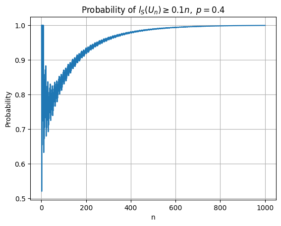
(a) Linear growth with positive probability before a fixed time

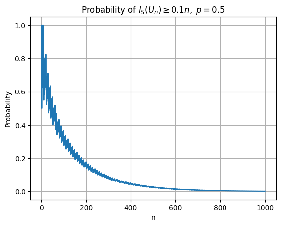
(b) Linear growth with high probability

Figure 1. Probability of linear growth for the exact length of random circuit

Thus we cannot expect a high probability linear growth for arbitrary random quantum circuits. The following is a list of problems we can discuss. In fact, we would like to discuss under what conditions on $S$, we can show the linear growth of complexity.

1. There exist $\Omega_{0}\subseteq\Omega$ with $\mathbb{P}(\Omega_{0})=1$, $L_{0}=L_{0}(d,S)\geq 1$ and $C:=C(d,S)>0$, such that for any $\omega\in\Omega_{0}$ and $l\leq L_{0}$, we have

   $$C_{S}(\Phi_{l}(\omega))\geq Cl.$$

2. There exist $\Omega_{0}\subseteq\Omega$ with $\mathbb{P}(\Omega_{0})\in(0,1)$, $L_{0}=L_{0}(d,S)\geq 1$ and $C:=C(d,S)>0$, such that for any $\omega\in\Omega_{0}$ and $l\leq L_{0}$, we have

   $$C_{S}(\Phi_{l}(\omega))\geq Cl.$$

3. There exist $L_{0}=L_{0}(d,S)\geq 1$ and $C:=C(d,S)>0$, such that for any $1\leq l\leq L_{0}$, there exists $\Omega_{l}\subseteq\Omega$ with $\mathbb{P}(\Omega_{l})\geq\delta(d,S,l)>0$ such that for any $\omega\in\Omega_{l}$, we have

   $$C_{S}(\Phi_{l}(\omega))\geq Cl.$$

In this section, we show that under the assumption that $S^{\prime}$ is a *-algebra and

(4.4) $$\|\Phi_{\nu}-E_{fix}\|_{2\to 2}\leq 1-\lambda,\ \lambda>0,$$

we have (3) holds.

Here is a diagram showing linear growth phenomenon in random quantum circuits:

$$\begin{array}[]{|c|c|}\hline\cr\text{Gate sets}&\text{Results}\\ \hline\cr\hbox{\multirowsetup Sufficiently connected circuits \cite[cite]{[\@@bibref{}{HFKEH}{}{}]}}&\\ &d=2^{n}.\forall l\leq 4^{n}-1,\mathbb{P}(l_{S}(\Phi_{l})\geq l/9-n/3)=1.\\ &\\ \hline\cr\hbox{\multirowsetup Universal gate sets \cite[cite]{[\@@bibref{}{Haferkamp23}{}{}]}}&\\ &\forall l\leq 2^{n/2},\mathbb{P}(l_{S,\delta}(\Phi_{l})\geq C(\delta,d)l)\geq 1-\exp(-O(l/n^{8})).\\ &\\ \hline\cr\hbox{\multirowsetup Theorem \ref{main}: arbitrary gate set with minor assumption}&\\ &\forall l\leq L_{0},\mathbb{P}(C_{S}(\Phi_{l})\geq l\frac{\varepsilon C_{S}(E_{fix})}{2L_{0}})\geq(\frac{1}{2}-\varepsilon)\frac{l}{l+L_{0}}.\\ &\\ \hline\cr\end{array}$$

Estimates for empirical mean

We will use empirical mean as an intermediate step. Suppose $\{U_{i}^{j}\}_{i,j\geq 1}$ are independent and identically distributed as $(S,\nu)$, then for any $i\geq 1$ and $M\geq 1$, define

(4.5) $$\Phi^{(M),i}(\rho):=\frac{1}{M}\sum_{j=1}^{M}Ad_{U_{i}^{j}}$$

For $M$ large enough, we expect $\|\Phi^{(M),i}-E_{fix}\|_{2\to 2}<1-\frac{\lambda}{2}$ with high probability. The quantitative version is a corollary of the following lemma:

Lemma 4.2.

There exists $C_{0}=C_{0}(S)>0$, such that for any $r>0$

(4.6) $$\mathbb{P}(\|\Phi^{(M),i}-\mathbb{E}\Phi^{(M),i}\|_{2\to 2}>r)\leq d^{2}\exp\bigg{(}-M\big{(}\frac{r}{2eC_{0}}\wedge(\frac{r}{2eC_{0}})^{2}\big{)}\bigg{)},$$

whenever $M\big{(}\frac{r}{2eC_{0}}\wedge(\frac{r}{2eC_{0}})^{2}\big{)}\geq 2.5$.

Proof.

First, note that for two probability measures $\nu_{1},\nu_{2}$ on $U(d)$,

(4.7) $$\|\Phi_{\nu_{1}}-\Phi_{\nu_{2}}\|_{2\to 2}=\|\int_{U(d)}U\otimes U^{*}d\nu_{1}-\int_{U(d)}U\otimes U^{*}d\nu_{1}\|_{\infty}.$$

Then

$$\|\Phi^{(M),i}-\mathbb{E}\Phi^{(M),i}\|_{2\to 2} =\|\frac{1}{M}\sum_{j=1}^{M}U_{i}^{j}\otimes U_{i}^{j*}-\int_{U(d)}U\otimes U^{*}d\nu\|_{\infty}$$

$$=\|\frac{1}{M}\sum_{j=1}^{M}\int_{U(d)}(U_{i}^{j}\otimes U_{i}^{j*}-U\otimes U^{*})d\nu\|_{\infty}.$$

Using Chebyshev inequality for $p\geq 2.5$ and applying non-commutative Bennett’s inequality [JZ13, Theorem 0.4], we have

$$\mathbb{P}(\|\Phi^{(M),i}-\mathbb{E}\Phi^{(M),i}\|_{2\to 2}>r)$$

$$\leq\frac{\mathbb{E}\|\frac{1}{M}\sum_{j=1}^{M}\int_{U(d)}(U_{i}^{j}\otimes U_{i}^{j*}-U\otimes U^{*})d\nu\|_{\infty}^{p}}{r^{p}}$$

$$\leq\frac{\mathbb{E}\operatorname{Tr}\big{(}|\frac{1}{M}\sum_{j=1}^{M}\int_{U(d)}(U_{i}^{j}\otimes U_{i}^{j*}-U\otimes U^{*})d\nu|^{p}\big{)}}{r^{p}}$$

$$=d^{2}\frac{\mathbb{E}\tau\big{(}|\frac{1}{M}\sum_{j=1}^{M}\int_{U(d)}(U_{i}^{j}\otimes U_{i}^{j*}-U\otimes U^{*})d\nu|^{p}\big{)}}{r^{p}}$$

$$\leq d^{2}(\frac{C_{0}(S)}{r})^{p}(\frac{p}{M}+\sqrt{\frac{p}{M}})^{p}.$$

For the last inequality, we take $x_{j}:=\int_{U(d)}(U_{i}^{j}\otimes U_{i}^{j*}-U\otimes U^{*})d\nu$, and apply non-commutative Bennett’s inequality:

$$\|\sum_{j=1}^{M}x_{j}\|_{p}\leq C^{\prime}\bigg{(}\sqrt{p}\big{\|}\big{(}\sum_{j=1}^{M}\mathbb{E}(x_{j}x_{j}^{*}+x_{j}^{*}x_{j})\big{)}^{\frac{1}{2}}\big{\|}_{p}+p\|(x_{j})\|_{L_{p}(l_{\infty})}\bigg{)}\leq C_{0}(S)(\sqrt{pM}+p).$$

Take

(4.8) $$p=\widetilde{c}M,\ \widetilde{c}:=\frac{r}{2eC_{0}}\wedge(\frac{r}{2eC_{0}})^{2},$$

we have

$$d^{2}(\frac{C_{0}(S)}{r})^{p}(\frac{p}{M}+\sqrt{\frac{p}{M}})^{p}$$

$$\leq d^{2}e^{-p}=d^{2}\exp\bigg{(}-M\big{(}\frac{r}{2eC_{0}}\wedge(\frac{r}{2eC_{0}})^{2}\big{)}\bigg{)}.$$

∎

If we take $r=\frac{\lambda}{2}$ in the above lemma, we get the following estimate:

Corollary 4.3.

For $M\geq\frac{10eC_{0}}{\lambda}$, we have

$$\mathbb{P}\big{(}\|\Phi^{(M),i}-E_{fix}\|_{2\to 2}\leq 1-\frac{\lambda}{2}\big{)}\geq 1-d^{2}\exp(-M\frac{\lambda}{4eC_{0}}).$$

Estimates of the complexity via empirical mean.

For two channels $\Phi,\Psi$, denote the product of channels as composition: $\Phi\cdot\Psi=\Phi\circ\Psi$. Then

(4.9) $$\prod_{i=1}^{l}\Phi^{(M),i}=\prod_{i=1}^{l}\frac{1}{M}\sum_{j=1}^{M}Ad_{U_{i}^{j}}=\frac{1}{M^{l}}\sum_{j_{1},\cdots,j_{l}=1}^{M}\prod_{i=1}^{l}Ad_{U_{i}^{j_{i}}}.$$

By convexity of complexity function and i.i.d. property $\mathbb{E}C_{S}(\Phi_{l})=\mathbb{E}C_{S}(\prod_{i=1}^{l}Ad_{U_{i}^{j_{i}}})$, we have

(4.10) $$\mathbb{E}C_{S}(\Phi_{l})\geq\mathbb{E}C_{S}(\frac{1}{M^{l}}\sum_{j_{1},\cdots,j_{l}=1}^{M}\prod_{i=1}^{l}Ad_{U_{i}^{j_{i}}})=\mathbb{E}C_{S}(\prod_{i=1}^{l}\Phi^{(M),i}).$$

[row sep=1.5cm,between origins, column sep=1.5cm,between origins] [4]$M$ virtual copies & U_1 U_2 ⋯ U_l

U_1^2 U_2^2 ⋯ U_l^2

⋯ ⋯ ⋯

U_1^M U_2^M ⋯ U_l^M

Moreover, for any $l\geq 1$, we have

(4.11) $$\|\prod_{i=1}^{l}\Phi^{(M),i}-E_{fix}\|_{2\to 2}=\|(\prod_{i=1}^{l-1}\Phi^{(M),i}-E_{fix})(\Phi^{(M),l}-E_{fix})\|_{2\to 2}$$

$$=\cdots=\|\prod_{i=1}^{l}(\Phi^{(M),i}-E_{fix})\|_{2\to 2}\leq\prod_{i=1}^{l}\|\Phi^{(M),i}-E_{fix}\|_{2\to 2}.$$

Thus using Corollary 4.3, we get

Lemma 4.4.

For $M\geq\frac{10eC_{0}}{\lambda}$, and $l\geq 1$, we have

(4.12) $$\mathbb{P}\big{(}\|\prod_{i=1}^{l}\Phi^{(M),i}-E_{fix}\|_{2\to 2}\leq(1-\frac{\lambda}{2})^{l}\big{)}\geq\big{(}1-d^{2}\exp(-M\frac{\lambda}{4eC_{0}})\big{)}^{l}.$$

Recall that for $\mathcal{N}_{fix}$-bimodule map $T$(here $S^{\prime}=\mathcal{N}_{fix}$), we have [GJL20a, Lemma 3.13]

(4.13) $$\|T^{2k}\|_{1\to\infty,cb}=\|T^{k}\|_{1\to 2,cb}^{2}=\|T^{k}\|^{2}_{2\to\infty,cb}$$

Thus

(4.14) $$\|\prod_{i=1}^{l}\Phi^{(M),i}-E_{fix}\|_{1\to\infty,cb}\leq I_{fix}\|\prod_{i=1}^{l}\Phi^{(M),i}-E_{fix}\|_{2\to 2}.$$

We get the following estimate:

Lemma 4.5.

For $M\geq\frac{10eC_{0}}{\lambda}$, and $l\geq 1$, we have

(4.15) $$\mathbb{P}\big{(}\|\prod_{i=1}^{l}\Phi^{(M),i}-E_{fix}\|_{1\to\infty,cb}\leq I_{fix}(1-\frac{\lambda}{2})^{l}\big{)}\geq\big{(}1-d^{2}\exp(-M\frac{\lambda}{4eC_{0}})\big{)}^{l}.$$

Proposition 1.

For any $l\geq\frac{\log I_{fix}}{-\log(1-\frac{\lambda}{2})}$, we have

(4.16) $$\mathbb{E}C_{S}(\Phi_{l})\geq\big{(}1-I_{fix}(1-\frac{\lambda}{2})^{l}\big{)}C_{S}(E_{fix}).$$

Proof.

From the previous lemma, for $M\geq\frac{10eC_{0}}{\lambda}$, we have

(4.17) $$(1-I_{fix}(1-\frac{\lambda}{2})^{l})E_{fix}\leq_{cp}\prod_{i=1}^{l}\Phi^{(M),i}\leq_{cp}(1+I_{fix}(1-\frac{\lambda}{2})^{l})E_{fix}$$

with probability $\big{(}1-d^{2}\exp(-M\frac{\lambda}{4eC_{0}})\big{)}^{l}$. Then by Lemma 2.6,

$$C_{S}(\prod_{i=1}^{l}\Phi^{(M),i})\geq(1-I_{fix}(1-\frac{\lambda}{2})^{l})C_{S}(E_{fix})$$

with probability $\big{(}1-d^{2}\exp(-M\frac{\lambda}{4eC_{0}})\big{)}^{l}$. Thus by (4.10),

(4.18) $$\mathbb{E}C_{S}(\Phi_{l})\geq\mathbb{E}C_{S}(\prod_{i=1}^{l}\Phi^{(M),i})\geq(1-I_{fix}(1-\frac{\lambda}{2})^{l})\big{(}1-d^{2}\exp(-M\frac{\lambda}{4eC_{0}})\big{)}^{l}C_{S}(E_{fix}).$$

Finally, let $M\to\infty$, we finish the proof. ∎

From the above Proposition, it is easy to see that for any $\varepsilon\in(0,\frac{1}{2})$, define

(4.19) $$L_{0}=L_{0}(\varepsilon)=\frac{\log\varepsilon-\log I_{fix}}{\log(1-\frac{\lambda}{2})}.$$

Then for any $l\geq L_{0}$, $\mathbb{E}C_{S}(\Phi_{l})\geq(1-\varepsilon)C_{S}(E_{fix})$. Moreover, by a simple argument, we can get the following:

Corollary 4.6.

For any $l\geq L_{0}$, and any $\delta>0$ small enough, we have

(4.20) $$\mathbb{P}(C_{S}(\Phi_{l})\geq\delta C_{S}(E_{fix}))\geq\frac{1-\varepsilon-\delta}{2}.$$

Proof.

For any $l\geq L_{0}$,

$$(1-\varepsilon)C_{S}(E_{fix})$$

$$\leq\mathbb{E}C_{S}(\Phi_{l})=\mathbb{E}(C_{S}(\Phi_{l});C_{S}(\Phi_{l})\geq\delta C_{S}(E_{fix}))+\mathbb{E}(C_{S}(\Phi_{l});C_{S}(\Phi_{l})<\delta C_{S}(E_{fix}))$$

$$\leq 2C_{S}(E_{fix})\mathbb{P}(C_{S}(\Phi_{l})\geq\delta C_{S}(E_{fix}))+\delta C_{S}(E_{fix}),$$

thus $\mathbb{P}(C_{S}(\Phi_{l})\geq\delta C_{S}(E_{fix}))\geq\frac{1-\varepsilon-\delta}{2}.$ ∎

Finally, we get the linear growth result:

Theorem 4.7.

For any $\varepsilon\in(0,\frac{1}{2})$, define

(4.21) $$L_{0}=L_{0}(\varepsilon)=\frac{\log\varepsilon-\log I_{fix}}{\log(1-\frac{\lambda}{2})}.$$

Then for any $l\leq L_{0}$, we have

(4.22) $$\mathbb{P}(C_{S}(\Phi_{l})\geq l\frac{\varepsilon C_{S}(E_{fix})}{2L_{0}})\geq(\frac{1}{2}-\varepsilon)\frac{l}{l+L_{0}}.$$

Proof.

For any $l\leq L_{0}$, choose $k\geq 1$, such that

(4.23) $$kl\geq L_{0},(k-1)l\leq L_{0}$$

Thus

$$\mathbb{P}(C_{S}(\Phi_{kl})\geq\varepsilon C_{S}(E_{fix}))\geq\frac{1}{2}-\varepsilon.$$

Note that we have

$$C_{S}(\Phi_{kl})\leq\sum_{s=1}^{k}C_{S}(\prod_{j=1}^{l}Ad_{U_{js}})$$

and for each $1\leq s\leq k$, $C_{S}(\prod_{j=1}^{l}Ad_{U_{js}})$ has the same distribution as $C_{S}(\Phi_{l})$. Thus

$$k\mathbb{P}(C_{S}(\Phi_{l})\geq\frac{1}{k}\varepsilon C_{S}(E_{fix}))\geq\mathbb{P}(C_{S}(\Phi_{kl})\geq\varepsilon C_{S}(E_{fix}))\geq\frac{1}{2}-\varepsilon.$$

Finally, using (4.23), we conclude the proof. ∎

Using dyadic arguments, we can show a slightly stronger result as follows:

Proposition 4.8.

There exists constants $c$ and $L$ depending on $S$ such that

(4.24) $$\mathbb{P} (\bigcap_{l=2^{k}<2^{L}}\{C_{S}(ad_{u_{i_{1}}}\cdots ad_{u_{i_{l}}})>cl\})>\frac{1}{4}2^{-L},$$

where for each $l=2^{k}$, $i_{1},i_{2}\cdots i_{l}$ is a consecutive sequence.

To prove the above Proposition, we need some standard probabilistic arguments. Recall that there exists $N=2^{L},\alpha>0,C>0$ such that

$$\mathbb{P}(C_{S}(Ad_{U_{1}}\cdots Ad_{U_{N}})\geq C)=\alpha>0$$

Given a random circuit with depth $N$, we partition the underlying probability space as

$$\Omega_{N}=\Omega_{N}^{1}\cup\Omega_{N}^{2},$$

where $\Omega_{N}^{1}=\{C_{S}(U_{N}\cdots U_{N/2+1})\geq C/2\},\Omega_{N}^{2}=\{C_{S}(U_{N/2}\cdots U_{1})\geq C/2\}$. Then we have

$$\mathbb{P}(\Omega_{N}^{1})\geq\alpha/2,\ \text{or}\ \mathbb{P}(\Omega_{N}^{2})\geq\alpha/2.$$

By induction we can show that

$$\mathbb{P} (\bigcap_{l=2^{k}<2^{L}}\{C_{S}(ad_{u_{i_{1}}}\cdots ad_{u_{i_{l}}})>C/2^{l}\})>\alpha 2^{-L},$$

Now take

$$c=\frac{C}{2^{L}L}=\frac{C}{N\log N},$$

the proposition follows.

4.2. Linear growth of Hamiltonian simulation

In this subsection, we illustrate our notion of complexity by an application to Hamiltonian simulation via ‘qDRIFT’ approach introduced by [Cam19].

The starting point is a Hamiltonian given by

$$H=\sum_{j=1}^{L}h_{j}H_{j}$$

where $H_{j}$ are some ‘more elementary’ components such that $\|H\|_{\infty}\leq 1$ and $h_{j}$ are some positive weights. Denote

(4.25) $$\lambda:=\sum_{j=1}^{L}h_{j}.$$

In this setting, we consider

(4.26) $$S=\{H_{j}|1\leq j\leq L\}$$

as a set of resources. The goal is to approximate the unitary $U(t)=\exp(itH)$ using a product of $U_{j}(\tau)=\exp(i\tau H_{j}),1\leq j\leq L$ up to some desired precision. This $\tau$ should be related to $t$. The number of elementary gates $U_{j}(\tau)=\exp(i\tau H_{j})$ used is called the cost of this quantum computation. In order to get an upper bound of the cost of $U(t)$, [Cam19] introduced the qDRIFT protocol as follows:

Suppose $N\geq 1$ is a fixed large integer and denote $\tau=\frac{t\lambda}{N}$. Assume $j_{1},j_{2},\cdots,j_{N}$ are i.i.d. random variables distributed as

(4.27) $$\mathbb{P}(j_{1}=j)=\frac{h_{j}}{\sum_{l=1}^{L}h_{l}},1\leq j\leq L.$$

Then the random unitary of length $N$ defined by

(4.28) $$V_{j_{1},\cdots,j_{N}}=\prod_{k=1}^{N}\exp(i\tau H_{j_{k}})$$

is a candidate to approximate $U(t)$ up to precision $\varepsilon$. In fact, The mean of $V_{j_{1},\cdots,j_{N}}$ is given as follows:

$$\mathbb{E}V_{j_{1},\cdots,j_{N}}\rho V_{j_{1},\cdots,j_{N}}^{*}=\Phi_{\tau}^{N}(\rho),$$

where for any $\tau>0$, $\Phi_{\tau}$ is defined by

(4.29) $$\Phi_{\tau}(\rho):=\sum_{j=1}^{L}p_{j}\exp(i\tau H_{j})\rho\exp(-i\tau H_{j}),$$

where $p_{j}:=\frac{h_{j}}{\lambda}=\frac{h_{j}}{\sum_{j=1}^{L}h_{j}}$.

It is shown in [Cam19] that an upper bound of the gate count $N$ is given by $O(\lambda^{2}t^{2}/\varepsilon)$ via the following estimate [Cam19, (B13)]:

(4.30) $$\|\Phi_{\tau}^{N}-Ad_{U(t)}\|_{\diamond}\leq 2\frac{\lambda^{2}t^{2}}{N}\exp(2\lambda t/N)$$

The goal in this subsection is to provide two sided estimates of

(4.31) $$C_{S}(Ad_{U(t)})=C_{S}(\exp(itH)\cdot\exp(-itH))$$

and it provides a lower bound on the cost of the quantum computation. In fact, we can show that it grows linearly in time before a threshold. The following is a general upper bounds exhibiting linear growth:

Theorem 4.9.

Define $\lambda=\sum_{j=1}^{L}h_{j}$. Then

(4.32) $$C_{S}(Ad_{U(t)})\leq\lambda t.$$

Proof.

First we claim that $C_{S}(\Phi_{\tau})\leq\tau$, where $\Phi_{\tau}$ is given by (4.29). In fact, using the Liouvillian representation of closed system

(4.33) $$\exp(itH)\rho\exp(-itH)=\exp(it[H,\rho]),$$

we have for any $x\in\mathcal{A}=\{x\in\mathcal{N}:E_{fix}(x)=0\}$ and $\mathcal{N}_{fix}=\{H_{j}|1\leq j\leq L\}^{\prime}$

$$\|(id-\Phi_{\tau}^{*})(x)\| =\|\sum_{j=1}^{L}p_{j}(x-\exp(-i\tau H_{j})x\exp(i\tau H_{j}))\|$$

$$\leq\sum_{j=1}^{L}p_{j}\|x-\exp(i\tau H_{j})x\exp(-i\tau H_{j})\|=\sum_{j=1}^{L}p_{j}\|x-\exp(i\tau[H_{j},x])\|$$

$$\leq\tau\sum_{j=1}^{L}p_{j}\|[H_{j},x]\|\leq\tau|||x|||_{S}.$$

Moreover, note that $\mathcal{N}_{fix}$ is given by the elements commuting with $H_{j}$ thus commuting with $H$, we have

(4.34) $$Ad_{U(t)}E_{fix}=E_{fix}Ad_{U(t)}=E_{fix},\Phi_{\tau}E_{fix}=E_{fix}.$$

Therefore, applying Lemma 2.7 and denote $\tau=\frac{\lambda t}{N}$, we have

$$C_{S}(Ad_{U(t)}) \leq C_{S}(\Phi_{\tau}^{N})+\|\Phi_{\tau}^{N}-Ad_{U(t)}\|_{\diamond}C_{S}(E_{fix})$$

$$\leq NC_{S}(\Phi_{\tau})+2\frac{\lambda^{2}t^{2}}{N}\exp(2\lambda t/N)C_{S}(E_{fix})$$

$$\leq N\tau+2\frac{\lambda^{2}t^{2}}{N}\exp(2\lambda t/N)C_{S}(E_{fix})$$

$$=\lambda t+2\frac{\lambda^{2}t^{2}}{N}\exp(2\lambda t/N)C_{S}(E_{fix}),$$

Then let $N\to\infty$ we get the conclusion. ∎

Note that the above upper bound is generically better than all the upper bounds of gate counts using Trotter formula and qDRIFT protocol, see [Cam19, Table I]. The reason is simple: our notion is a lower bound of (approximate) gate length. The following example shows that the complexity $\lambda t$ is also sharp:

Example 4.10.

Consider $n$-qubit system and the Hamiltonian $H=\sum_{j=1}^{n}(X_{j}+Y_{j})$. Then the resource set is given by $S=\{X_{j},Y_{j}:1\leq j\leq n\}$ and the complexity of $Ad_{e^{iHt}}$ has lower bound $cnt$ for some universal constant $c>0$ and small $t>0$. One can check directly by choosing $f=\sum_{j}X_{j}$.

A lower bound on the complexity of $Ad_{U(t)}$ can also be established, and it exhibits linear growth for small time as long as $H\neq 0$.

Theorem 4.11.

Suppose $H\neq 0$, then for $0\leq t\leq\frac{1}{4(e-2)\|H\|_{\infty}}$, we have

(4.35) $$C_{S}(Ad_{U(t)})\geq\frac{1}{2}\delta t,$$

where $\delta>0$ is given by

(4.36) $$\delta:=\sup_{x:E_{fix}(x)=0}\frac{\|[H,x]\|}{\sup_{j}\|[H_{j},x]\|}.$$

Proof.

By the definition of $C_{S}(Ad_{U(t)})$, for any $x\in\mathcal{A}=\{x\in\mathcal{N}:E_{fix}(x)=0\}$, we have

(4.37) $$C_{S}(Ad_{U(t)})\sup_{j}\|[H_{j},x]\|\geq\|x-Ad_{U(t)}^{*}(x)\|=\|x-e^{-iHt}xe^{iHt}\|.$$

We aim to establish a lower bound of $\|x-e^{-iHt}xe^{iHt}\|$. For any state $\rho$, we have

$$\|x-e^{-iHt}xe^{iHt}\| \geq|\operatorname{tr}(\rho(x-e^{iHt}xe^{-iHt}))|=|\operatorname{tr}(\rho(x-e^{it[H,x]})|$$

$$=|\operatorname{tr}(\rho(i[H,x]t+\sum_{n\geq 2}\frac{(it)^{n}}{n!}\delta_{H}^{n}(x))|$$

$$\geq|\operatorname{tr}(\rho[H,x])|t-|\operatorname{tr}(\rho(\sum_{n\geq 2}\frac{(it)^{n}}{n!}\delta_{H}^{n}(x)))|,$$

where $\delta_{H}^{n}(x)$ is defined by $\delta_{H}^{0}(x)=x,\delta_{H}^{n+1}=[H,\delta_{H}^{n}(x)]$. We need to get an upper bound

$$|\operatorname{tr}(\rho(\sum_{n\geq 2}\frac{(it)^{n}}{n!}\delta_{H}^{n}(x)))| \leq\sum_{n\geq 2}\frac{t^{n}}{n!}|\operatorname{tr}(\rho\delta_{H}^{n}(x))|$$

$$\leq\sum_{n\geq 2}\frac{t^{n}(2\|H\|)^{n-1}}{n!}\|[H,x]\|$$

$$=(e^{2\|H\|t}-1-2\|H\|t)\frac{\|[H,x]\|}{2\|H\|}$$

$$\leq(e-2)(2\|H\|t)^{2}\frac{\|[H,x]\|}{2\|H\|}=2(e-2)\|H\|\|[H,x]\|t^{2}$$

if $2\|H\|t\leq 1$. Here we used an elementary estimate: $e^{a}-a-1\leq(e-2)a^{2}$ for $a\in[0,1]$ in the last inequality and $\|\delta_{H}^{n}(x)\|\leq(2\|H\|)^{n-1}\|[H,x]\|$ in the second inequality. Since $\rho$ is arbitrary, we can choose $\rho$ such that $|\operatorname{tr}(\rho[H,x])|$ approaches $\|[H,x]\|$. Then we have

$$\|x-e^{-iHt}xe^{iHt}\| \geq\|[H,x]\|t\big{(}1-2(e-2)\|H\|t\big{)}\geq\frac{\|[H,x]\|}{2}t,$$

if $4(e-2)\|H\|t\leq 1$. In summary, we showed that

(4.38) $$C_{S}(Ad_{U(t)})\sup_{j}\|[H_{j},x]\|\geq\frac{\|[H,x]\|}{2}t,$$

if $4(e-2)\|H\|t\leq 1$. ∎

Estimates of complexity of $\Phi_{\tau}$

Note that if the Hamiltonian $H$ is non-zero, the complexity of $e^{itH}$ grows linearly. In this section, we showed that the complexity of approximate random unitary $\Phi_{\tau}$ has a lower bound, which indicates that $\Phi_{\tau}$ can have large complexity even it approximates identity(when $H=0$).

We first need some preliminary estimates on the spectral gap on mixed unitary channels. In the remaining part of this section, we assume $S=\{H_{1},\cdots,H_{L}\}$ and denote $\mathcal{N}_{fix}=S^{\prime}$.

Lemma 4.12.

Suppose $u_{1},\cdots,u_{m}$ are unitaries which commute with $\mathcal{N}_{fix}$, i.e., $Ad_{u_{j}}E_{fix}=E_{fix}$. Suppose $\Phi(x):=\sum_{j=1}^{m}p_{j}Ad_{u_{j}}$ with $p_{j}>0,\sum_{j}p_{j}=1$, and $x_{0}\in\mathcal{N}_{fix}^{\perp}$ with $\|x_{0}\|_{2}=1$ such that

(4.39) $$\|\Phi(x_{0})\|_{2}\geq 1-\varepsilon,$$

for some $\varepsilon>0$. Then for any $j\neq k$,

(4.40) $$\|Ad_{u_{j}}(x_{0})-Ad_{u_{k}}(x_{0})\|_{2}\leq\sqrt{2}(\sqrt{\frac{1-p_{j}}{p_{j}}}+\sqrt{\frac{1-p_{k}}{p_{k}}})\sqrt{\varepsilon}.$$

Proof.

The proof is a corollary of the following Hilbert space argument via Cauchy-Schwartz inequality: suppose $\mathcal{K}$ is a Hilbert space with inner product $\langle\cdot,\cdot\rangle$, if $x,y\in\mathcal{K}$, $p\in(0,1)$ such that $\|x\|=1,\|y\|\leq 1$ and $\|px+(1-p)y\|\geq 1-\varepsilon$, then

(4.41) $$\|x-y\|\leq\sqrt{\frac{2\varepsilon}{p(1-p)}}.$$

To show (4.41), note that

$$\|px+(1-p)y\|^{2} =\langle px+(1-p)y,px+(1-p)y\rangle$$

$$=p^{2}\|x\|^{2}+(1-p)^{2}\|y\|^{2}+2p(1-p)Re(\langle x,y\rangle)\geq(1-\varepsilon)^{2},$$

thus

$$\|x-y\|^{2} =\|x\|^{2}+\|y\|^{2}-2Re(\langle x,y\rangle)$$

$$\leq 1+\|y\|^{2}-\frac{(1-\varepsilon)^{2}-p^{2}-(1-p)^{2}\|y\|^{2}}{p(1-p)}=1+\frac{1}{p}\|y\|^{2}+\frac{p}{1-p}-\frac{(1-\varepsilon)^{2}}{p(1-p)}$$

$$\leq\frac{2\varepsilon}{p(1-p)}.$$

Now we denote$p=p_{j}$, $x=Ad_{u_{j}}(x_{0})$, $y=\frac{1}{1-p_{j}}\sum_{r\neq j}p_{r}Ad_{u_{r}}(x_{0})$. By triangle inequality, $\|y\|_{2}\leq 1$. Apply (4.41), we have

$$\|x-y\|_{2}=\|Ad_{u_{j}}(x_{0})-\frac{1}{1-p_{j}}\sum_{r\neq j}p_{r}Ad_{u_{r}}(x_{0})\|_{2}\leq\sqrt{\frac{2\varepsilon}{p_{j}(1-p_{j})}},$$

thus multiplying by $(1-p_{j})$,

$$\|(1-p_{j})Ad_{u_{j}}(x_{0})-\sum_{r\neq j}p_{r}Ad_{u_{r}}(x_{0})\|_{2}=\|Ad_{u_{j}}(x_{0})-\Phi(x_{0})\|_{2}\leq\sqrt{\frac{2\varepsilon(1-p_{j})}{p_{j}}}.$$

Finally by triangle inequality, we have

$$\|Ad_{u_{j}}(x_{0})-Ad_{u_{k}}(x_{0})\|_{2} \leq\|Ad_{u_{j}}(x_{0})-\Phi(x_{0})\|_{2}+\|Ad_{u_{j}}(x_{0})-\Phi(x_{0})\|_{2}$$

$$\leq\sqrt{2}(\sqrt{\frac{1-p_{j}}{p_{j}}}+\sqrt{\frac{1-p_{k}}{p_{k}}})\sqrt{\varepsilon}.$$

∎

We denote

(4.42) $$C(p_{j},p_{k}):=\sqrt{2}(\sqrt{\frac{1-p_{j}}{p_{j}}}+\sqrt{\frac{1-p_{k}}{p_{k}}}).$$

Back to our setting, since we are dealing with mixed unitary channels where the unitary is given by $\exp(i\tau H)$, the following lemma would be helpful:

Lemma 4.13.

Suppose $H_{0}\neq 0$ is a self-adjoint operator. Then for any $|\tau|\leq\frac{1}{4\|H_{0}\|_{2}(e-2)}$, we have

(4.43) $$\|[\exp(i\tau H),x]\|_{2}\geq\frac{1}{2}\|[H_{0},x]\|_{2}|\tau|.$$

Proof.

The proof follows the same procedure as Theorem 4.11. The only difference is we use the duality $L_{2}^{*}\cong L_{2}$ instead of $L_{1}^{*}\cong L_{\infty}$. We include the proof for completeness. For any $y\in L_{2}(\mathbb{M}_{d})$ with $\|y\|_{2}=1$, we have

$$\|[\exp(i\tau H),x]\|_{2} \geq\|\langle y,[\exp(i\tau H),x]\rangle\|$$

$$\geq|\tau||\langle y,[H_{0},x]\rangle|-\sum_{n\geq 2}\frac{|\tau|^{n}}{n!}|\langle y,\delta_{H_{0}}^{n}(x)\rangle|$$

Note that for any $z\in L_{2}(\mathbb{M}_{d})$, we have $\|[H_{0},z]\|_{2}=\|H_{0}z-zH_{0}\|_{2}\leq 2\|H_{0}\|_{2}\|z\|_{2}$, by induction we have

$$\|\delta_{H_{0}}(x)\|_{2}=\|[H_{0},[H_{0},\cdots[H_{0},x]]]\|_{2}\leq(2\|H_{0}\|_{2})^{n-1}\|[H_{0},x]\|_{2}.$$

Therefore, by Cauchy-Schwartz inequality,

$$\|[\exp(i\tau H),x]\|_{2} \geq|\tau||\langle y,[H_{0},x]\rangle|-\sum_{n\geq 2}\frac{|\tau|^{n}}{n!}|\langle y,\delta_{H_{0}}^{n}(x)\rangle|$$

$$\geq|\tau||\langle y,[H_{0},x]\rangle|-\sum_{n\geq 2}\frac{(2\|H_{0}\|_{2}|\tau|)^{n}}{n!}\frac{\|[H_{0},x]\|_{2}}{2\|H_{0}\|_{2}}$$

$$=\|[H_{0},x]\|_{2}\big{(}|\tau|-\frac{e^{2\|H_{0}\|_{2}|\tau|}-1-2\|H_{0}\|_{2}|\tau|}{2\|H_{0}\|_{2}}\big{)}$$

$$\geq\frac{1}{2}\|[H_{0},x]\|_{2}|\tau|,$$

for any $|\tau|\leq\frac{1}{4\|H_{0}\|_{2}(e-2)}$, where we used the same elementary inequality $e^{a}-a-1\leq(e-2)a^{2}$ for $a\in[0,1]$. ∎

The next proposition enables us to connect the spectral gap of a symmetric Lindbladian to the spectral gap of mixed unitary channels:

Proposition 4.14.

Suppose $\mathcal{L}$ is a symmetric Lindbladian given by

(4.44) $$\mathcal{L}(x)=\sum_{j=1}^{L}[H_{j},[H_{j},x]]$$

with spectral gap

$$\lambda_{2}(\mathcal{L}):=\inf_{x\in\mathcal{N}_{fix}^{\perp}}\frac{\langle\mathcal{L}(x),x\rangle}{\|x\|_{2}^{2}}>0.$$

Then any mixed unitary channel $\widetilde{\Phi}_{\tau}(x):=p_{0}x+\sum_{j=1}^{L}p_{j}Ad_{e^{i\tau H_{j}}}(x)$ with $\sum_{j=0}^{L}p_{j}=1,p_{j}>0$ has spectral estimate given by

(4.45) $$\|\widetilde{\Phi}_{\tau}-E_{fix}\|_{2\to 2}\leq 1-\tau^{2}\frac{\lambda_{2}(\mathcal{L})}{4\sum_{j=1}^{m}C(p_{0},p_{j})^{2}}$$

for $|\tau|\leq\min_{j}\frac{1}{4\|H_{j}\|_{2}(e-2)}$.

Proof.

Pick $x_{0}\in\mathcal{N}_{fix}^{\perp}$ with $\|x_{0}\|_{2}=1$, such that $\|\widetilde{\Phi}_{\tau}(x_{0})\|_{2}=1-\varepsilon$. Then applying Lemma 4.12 for $u_{0}=id,u_{j}=e^{i\tau H_{j}}$, we have

$$\|x_{0}-Ad_{e^{i\tau H_{j}}}(x_{0})\|_{2}\leq C(p_{0},p_{j})\sqrt{\varepsilon}$$

Moreover, by Lemma 4.13, for $|\tau|\leq\frac{1}{4\|H_{j}\|_{2}(e-2)}$,

(4.46) $$\frac{|\tau|}{2}\|H_{j},x_{0}\|_{2}\leq\|x_{0}-Ad_{e^{i\tau H_{j}}}(x_{0})\|_{2}\leq C(p_{0},p_{j})\sqrt{\varepsilon}$$

By direct calculation, we have

$$\lambda_{2}(\mathcal{L}) =\lambda_{2}(\mathcal{L})\|x_{0}\|^{2}\leq\langle\mathcal{L}(x_{0}),x_{0}\rangle=\sum_{j=1}^{L}\langle[H_{j},[H_{j},x_{0}]],x_{0}\rangle=\sum_{j=1}^{L}\|[H_{j},x_{0}]\|_{2}^{2}$$

$$\leq\sum_{j=1}^{L}\frac{4C(p_{0},p_{j})^{2}\varepsilon}{\tau^{2}},$$

which implies

(4.47) $$\varepsilon\geq\frac{\tau^{2}\lambda_{2}(\mathcal{L})}{4\sum_{j}C(p_{0},p_{j})^{2}}$$

for $|\tau|\leq\min_{j}\frac{1}{4\|H_{j}\|_{2}(e-2)}$. Take $x_{0}$ to be norm achieving element and we are done. ∎

Finally, we are able to provide a lower bound for $\Phi_{\tau}$:

Theorem 4.15.

There exists a universal constant $C>0$, such that for $|\tau|\leq\min_{j}\frac{1}{4(e-2)\|H_{j}\|_{2}}$, we have

(4.48) $$C_{S}^{cb}(\Phi_{\tau})\geq C_{S}(\Phi_{\tau})\geq C\tau^{2}$$

Proof.

The proof follows from standard return time argument. For any $k\geq 1$, we have

$$\|\Phi^{*k}-E_{fix}:L_{1}(\mathbb{M}_{d})\to L_{1}^{\infty}(\mathcal{N}_{fix}\subset\mathbb{M}_{d})\|_{cb}$$

$$\leq\|id:L_{1}(\mathbb{M}_{d})\to L_{1}^{2}(\mathcal{N}_{fix}\subset\mathbb{M}_{d})\|_{cb}\|\Phi^{*k}-E_{fix}\|_{2\to 2}\|id:L_{2}(\mathbb{M}_{d})\to L_{2}^{\infty}(\mathcal{N}_{fix}\subset\mathbb{M}_{d})\|_{cb}$$

$$\leq C^{cb}(\mathcal{N}_{fix}:\mathbb{M}_{d})\big{(}1-\tau^{2}\frac{\lambda_{2}(\mathcal{L})}{4\sum_{j=1}^{m}C(p_{0},p_{j})^{2}}\big{)}^{k}.$$

Denote $\widetilde{\Phi}_{\tau}=\frac{1}{2}\Phi_{\tau}+\frac{1}{2}I$, using Lemma 2.5, and convexity of complexity function, we have for any $\varepsilon\in(0,1)$,

$$C_{S}^{cb}(\Phi_{\tau})\geq 2C_{S}^{cb}(\widetilde{\Phi}_{\tau})\geq 2\frac{1-\varepsilon}{k_{ret}^{cb}(\varepsilon,\Phi_{\tau})}C_{S}^{cb}(E_{fix})\geq 2\frac{\log(1-\tau^{2}\frac{\lambda_{2}(\mathcal{L})}{4\sum_{j=1}^{m}C(p_{0},p_{j})^{2}})}{\log(\frac{\varepsilon}{C^{cb}(\mathcal{N}_{fix}:\mathbb{M}_{d})})}(1-\varepsilon)C_{S}^{cb}(E_{fix}).$$

Note that $\log(1-O(\tau^{2}))\sim\tau^{2}$ and we are done. ∎

5. Linear growth of Lipschitz complexity for open quantum systems

5.1. Discrete gates as resource

Suppose $S=\{U_{1},\cdots,U_{l}\}\subset\mathbb{M}_{d}$ is a set of unitaries. Moreover, we assume it to be symmetric. The set of channels we will consider is $CP_{S}(\mathbb{M}_{d})$. For dynamics, recall that the Hamiltonian-free Lindblad generator is given by the jump operators from the above gate set. Recall that the Lipschitz norm is given as follows:

(5.1) $$|||X|||_{S}:=\sup_{j=1,\cdots,l}\|[U_{j},X]\|_{\infty}.$$

The mean zero space is given by $\mathcal{A}=\{x\in\mathbb{M}_{d}:E_{S^{\prime}}(x)=0\}$. The complete complexity of any channel $\Phi$ is given by

$$C_{S}^{cb}(\Phi):=\|\Phi^{*}-id:(\mathcal{A},|||\cdot|||_{S})\to\mathbb{M}_{d}\|_{cb}.$$

Suppose we are given a unitary channel from $S$, i.e.,

$$\Phi_{\mu}:=\sum_{i}\mu_{i}U_{i}\cdot U_{i}^{*},$$

where $\{\mu_{i}\}_{i}$ is a probability measure. Then we are able to give an upper bound of the complexity of the dynamics driven by $\Phi_{\mu}$:

Proposition 5.1.

The evolution

(5.2) $$T_{t}:=\exp(t(\Phi_{\mu}-I))$$

satisfies

(5.3) $$C_{S}^{cb}(T_{t})\leq t.$$

Proof.

First we claim that

(5.4) $$C_{S}^{cb}(\Phi_{\mu})\leq 1.$$

In fact, for any $X\in\mathcal{A}$,

$$\|\Phi_{\mu}^{*}(X)-X\|_{cb} =\|\sum_{i}\mu_{i}(U_{i}^{*}XU_{i}-X)\|_{cb}\leq\sum_{i}\mu_{i}\|U_{i}^{*}XU_{i}-X\|_{cb}$$

$$=\sum_{i}\mu_{i}\|U_{i}^{*}X-XU_{i}^{*}\|_{cb}=\sum_{i}\mu_{i}\|[U_{i}^{*},X]\|_{cb}\leq|||X|||^{cb}_{S}.$$

Recall that

(5.5) $$T_{t}:=\exp(t(\Phi_{\mu}-I))=\sum_{k=0}^{\infty}\frac{t^{k}}{k!}e^{-t}\Phi_{\mu}^{k}.$$

Then by convexity and subadditivity under concatenation, we have

$$C_{S}^{cb}(T_{t})\leq\sum_{k=0}^{\infty}\frac{t^{k}}{k!}e^{-t}C_{S}^{cb}(\Phi_{\mu}^{k})\leq\sum_{k=0}^{\infty}\frac{t^{k}}{k!}e^{-t}k=t.$$

∎

For the lower bound estimate, we first connect the complexity of a class of channels to its return time to its fixed point.

Suppose $\Phi$ is an arbitrary quantum channel with the same fixed point algebra $\mathcal{N}_{fix}=S^{\prime}$ and we define its (complete) return time $t^{(cb)}(\varepsilon,\Phi)$:

(5.6) $$t^{(cb)}(\varepsilon,\Phi):=\inf\{k\in\mathbb{N}:\|(\Phi^{*})^{k}-E_{fix}\|^{(cb)}_{\infty\to\infty}\leq\varepsilon\},$$

where $E_{fix}=E_{S^{\prime}}$ is the trace-preserving conditional expectation onto the fixed point algebra.

To provide a lower bound, we need to assume $\Phi_{\mu}$ is symmetric such that we get bounded return time. The dynamical evolution $T_{t}=\exp(t(\Phi_{\mu}-id))$ converges to $E_{fix}$ as $t$ goes to infinity and moreover [GJLL22],

(5.7) $$k^{cb}(\frac{1}{2}):=\inf\{t>0:\|T_{t}-E_{fix}\|_{cb}\leq\frac{1}{2}\}<\infty.$$

Now we are ready to provide the lower bound of complexity of $T_{t}$:

Theorem 5.2.

Suppose $T_{t}$ given by (5.2) is symmetric, i.e., $T_{t}=T_{t}^{*}$, then

(5.8) $$C^{cb}_{Lip_{L}}(T_{t})\asymp\begin{cases}t,\ t\leq k^{cb}(\frac{1}{2}),\\ C^{cb}_{S}(E_{fix}),\ t\geq k^{cb}(\frac{1}{2}).\end{cases}$$

Here $a\asymp b$ means there exist universal constants $C_{1},C_{2}>0$ such that $C_{1}b\leq a\leq C_{2}b$.

Proof.

We only show the case for $C_{S}(T_{t})$, and the complete version has exactly the same proof. If $t\leq k^{cb}(\frac{1}{2})$, the upper bound follows from the previous proposition. For the lower bound, we choose $k\geq 1$ such that

(5.9) $$(k-1)t\leq k^{cb}(\frac{1}{2})\leq kt.$$

Then

$$C_{S}(E_{fix}) =\|E_{fix}-id:(\mathcal{A},|||\cdot|||_{S})\to L_{\infty}(\mathbb{M}_{d})\|$$

$$=\|E_{fix}-(T_{t})^{k}+(T_{t})^{k}-id:(\mathcal{A},|||\cdot|||_{S})\to L_{\infty}(\mathbb{M}_{d})\|$$

$$\leq C_{S}(T_{t}^{k})+\|E_{fix}-(T_{t})^{k}:(\mathcal{A},|||\cdot|||_{S})\to L_{\infty}(\mathbb{M}_{d})\|$$

$$\leq kC_{S}(T_{t})+C_{S}(E_{fix})\|E_{fix}-(T_{t})^{k}\|_{\infty\to\infty}$$

$$\leq kC_{S}(T_{t})+\frac{1}{2}C_{S}(E_{fix}).$$

Therefore,

$$C_{S}(T_{t})\geq\frac{C_{S}(E_{fix})}{2k}\geq\frac{tC_{S}(E_{fix})}{2(k^{cb}(\frac{1}{2})/t+1)}\geq\frac{tC_{S}(E_{fix})}{4k^{cb}(\frac{1}{2})},$$

where in the last two inequalities, we used (5.9) and the fact that $t\leq k^{cb}(\frac{1}{2})$.

If $t\geq k^{cb}(\frac{1}{2})$, we have $\|E_{fix}-T_{t}\|_{\infty\to\infty}\leq\frac{1}{2}$,

$$C_{S}(E_{fix}) =\|E_{fix}-id:(\mathcal{A},|||\cdot|||_{S})\to L_{\infty}(\mathbb{M}_{d})\|$$

$$=\|E_{fix}-T_{t}+T_{t}-id:(\mathcal{A},|||\cdot|||_{S})\to L_{\infty}(\mathbb{M}_{d})\|$$

$$\leq C_{S}(T_{t})+\frac{1}{2}C_{S}(E_{fix}),$$

thus $C_{S}(T_{t})\geq\frac{1}{2}C_{S}(E_{fix})$. Similarly, we can show that $C_{S}(T_{t})\leq\frac{3}{2}C_{S}(E_{fix})$, by bounding $C_{S}(T_{t})$. ∎

5.2. Continuous case: infinitesimal generators as resource

We take $\mathcal{N}=\mathbb{M}_{d}$ and $L:\mathbb{M}_{d}\to\mathbb{M}_{d}$ as a self-adjoint Lindbladian, i.e.,

(5.10) $$L(x)=\sum_{j}\big{(}a_{j}xa_{j}-\frac{1}{2}(a_{j}^{2}x+xa_{j}^{2})\big{)},$$

where $a_{j}$ are self-adjoint. Denote $\tau$ as the normalized trace, $\mathcal{N}_{fix}=\{X\in\mathbb{M}_{d}:[a_{j},X]=0,\forall j\}$ and $E_{fix}$ is the trace-preserving conditional expectation onto $\mathcal{N}_{fix}$. The resource set, denoted by $\Delta$ is given by

(5.11) $$\Delta:=\{a_{j}\}.$$

We can define the resource-dependent Lipschitz norm and complexity $|||\cdot|||_{\Delta},C_{\Delta}$ as before. The mean 0 space is given by $\mathcal{A}=\{X\in\mathbb{M}_{d}:E_{fix}(X)=0\}.$ In order to estimate $C_{\Delta}(T_{t})$, where $T_{t}=e^{tL}$, we need to introduce the another Lipschitz norm, induced by the gradient form. Recall the gradient form of $L$ is defined by

(5.12) $$\Gamma_{L}(x,y):=L(x^{*}y)-x^{*}L(y)-L(x^{*})y,\ x,y\in\mathbb{M}_{d}.$$

We define the Lipschitz norm via the gradient form:

(5.13) $$|||X|||_{\Gamma}:=\max\{\|\Gamma_{L}(X,X)\|_{\infty}^{\frac{1}{2}},\|\Gamma_{L}(X^{*},X^{*})\|_{\infty}^{\frac{1}{2}}\}.$$

Recall that for any $X\in\mathcal{A}$, $|||X|||_{\Delta}=\sup_{j}||[a_{j},X]||=\sup_{j}||[a_{j},X^{*}]||=|||X^{*}|||_{\Delta}$, by definition, we can show that

(5.14) $$|||X|||_{\Gamma}\leq\sqrt{|\Delta|}\cdot|||X|||_{\Delta}.$$

The Lipschitz norm $|||\cdot|||_{\Gamma}$ induces a quantum metric on the state space:

(5.15) $$\|\rho\|_{\Gamma^{*}}=\sup\{|\tau(\rho X)|\big{|}E_{fix}(X)=0,\|X\|_{\Gamma}\leq 1\}.$$

To establish an upper bound, we make use of modified logarithmic Sobolev inequality. Recall that $\{T_{t}:=\exp(tL)\}$ satisfies the $\lambda$-modified logarithmic Sobolev inequality ($\lambda$-MLSI) if there exists a constant $\lambda>0$ such that the relative entropy has exponential decay:

(5.16) $$D(T_{t}\rho\|E_{fix}\rho)\leq e^{-\lambda t}D(\rho\|E_{fix}\rho)$$

The largest constant $\lambda$ for which the relative entropy decays exponentially is denoted as $\text{MLSI}(L)$ (the MLSI constant of $L$). We denote the best constant as $\text{CLSI}(L)$ if we consider the complete version. By definition, the fixed point algebra $\mathcal{N}_{fix}$ of $\{T_{t}\}_{t\geq 0}$ is tracial-orthogonal to the Lipschitz subspace $\mathcal{A}$.

Recall the notation of index of a von Neumann subalgebra $\mathcal{M}\subset\mathcal{N}$. Let $E_{\mathcal{M}}:\mathcal{N}\rightarrow\mathcal{M}$ be the conditional expectation onto $M$ (with respect to the trace):

(5.17) $$\text{Ind}(\mathcal{N}:\mathcal{M}):=\inf\{\alpha>0:\rho\leq\alpha E_{\mathcal{M}}^{*}(\rho)\text{ , }\forall\rho\in L_{1}(\mathcal{N})_{+}\}\hskip 2.84544pt.$$

For example, $\text{Ind}(M_{n}(\mathbb{C}):\mathbb{C})=n$ and $\text{Ind}(M_{n}(\mathbb{C}):\ell_{\infty}^{n})=n$. Hence the index is a proper notion of relative size of $\mathcal{M}$ in $\mathcal{N}$.

We recall the following result from [GJL20a, Corollary 6.8]:

Proposition 5.3.

If the Lindbladian $L$ generates a semigroup that satisfies $\lambda$-MLSI, then we have:

(5.18) $$||\rho-E_{fix}^{*}\rho||_{\Gamma^{*}}\leq 4\sqrt{\frac{2D(\rho\|E^{*}_{fix}\rho)}{\lambda}}$$

for any state $\rho$, where $||\cdot||_{\Gamma^{*}}$ is dual to the Lipschitz norm $|||\cdot|||_{Lip_{L}}$.

Note that in the tracial setting, $E_{fix}^{*}=E_{fix}$. Then we can get an upper estimate for the expected length:

Lemma 5.4.

The expected length of $\mathcal{A}$ is bounded above by:

(5.19) $$EL_{\Delta}^{cb}(\mathcal{A}):=C_{\Delta}^{cb}(E_{fix})\leq 4\sqrt{\frac{2|\Delta|\sup_{\rho}D^{cb}(\rho\|E_{fix}\rho)}{\text{CLSI}(L)}}\leq 4\sqrt{\frac{2|\Delta|\log(\text{Ind}^{cb}(\mathcal{N}:\mathcal{N}_{fix}))}{\text{CLSI}(L)}}.$$

Proof.

We only prove the case for $EL_{\Delta}(\mathcal{A})$ and the complete version follows from the same argument.

First, using the relation between the two Lipschitz norms $|||\cdot|||_{\Gamma}$ and $|||\cdot|||_{\Delta}$, we have:

(5.20) $$||id:(\mathcal{A},|||\cdot|||_{\Delta})\rightarrow(\mathcal{A},|||\cdot|||_{\Gamma})||\leq\sqrt{|\Delta|}\hskip 2.84544pt.$$

Then using the definition of expected length, we have:

(5.21) $$\begin{split}EL_{\Delta}(\mathcal{A})&=||id:(\mathcal{A},|||\cdot|||_{\Delta})\rightarrow\mathcal{N}||\leq\sqrt{|\Delta|}||id:(\mathcal{A},|||\cdot|||_{\Gamma})\rightarrow\mathcal{N}||\\ &=\sqrt{|\Delta|}\cdot||E_{fix}-id:(\mathcal{A},|||\cdot|||_{\Gamma})\rightarrow\mathcal{N}||\\ &=\sqrt{|\Delta|}\cdot||E^{*}_{fix}-id:L_{1}(\mathcal{N})\rightarrow(\mathcal{A},|||\cdot|||_{\Gamma})^{*}||\\ &\leq 4\sqrt{\frac{2|\Delta|\sup_{\rho}D(\rho\|E_{fix}\rho)}{\text{MLSI}(L)}}\end{split}$$

where the equation in the second line follows from $E_{fix}(\mathcal{A})=0$ and the inequality follows from Proposition 5.3. This gives the first upper bound. For the second upper bound, we used the result in [GJL20b]:

(5.22) $$D_{\mathcal{N}_{fix}}\leq\log\text{Ind}(\mathcal{N}:\mathcal{N}_{fix})\hskip 2.84544pt.$$

where $D_{\mathcal{N}_{fix}}:=\sup_{\rho:\operatorname{tr}\rho=1}D(\rho|E^{*}_{fix}\rho)$ is the maximum entropy [GJL20b, GR22] and the maximum entropy is bounded above by the log-index [GJL20b, GR22]. ∎

Combining the above lemma and the elementary property (4) of Lemma 2.4, the upper estimate of $C_{\Delta}^{cb}(T_{t})$ is clear:

Theorem 5.5.

Suppose $T_{t}=\exp(tL)$ where $L$ is given by (5.10). Then we have the following upper estimate: for any $t\geq 0$,

(5.23) $$C_{\Delta}^{cb}(T_{t})\leq 4\sqrt{\frac{2|\Delta|\log(\text{Ind}^{cb}(\mathcal{N}:\mathcal{N}_{fix}))}{\text{CLSI}(L)}}\|L\|_{cb}t.$$

Since the return time argument works for any symmetric quantum channel, the lower bound can also be derived, as in the last subsection:

Theorem 5.6.

Define the return time for $T_{t}=\exp(tL)$ with L given by (5.10):

(5.24) $$k^{cb}(\frac{1}{2}):=\inf\{t>0:\|T_{t}-E_{fix}\|_{cb}\leq\frac{1}{2}\}<\infty.$$

Then the lower bound estimate of $C_{\Delta}^{cb}(T_{t})$ is given as follows:

(5.25) $$C_{\Delta}^{cb}(T_{t})\geq\frac{tC_{S}(E_{fix})}{4k^{cb}(\frac{1}{2})},t\leq k^{cb}(\frac{1}{2}).$$

(5.26) $$C_{\Delta}^{cb}(T_{t})\asymp C^{cb}_{\Delta}(E_{fix}),\ t>k^{cb}(\frac{1}{2}).$$

6. Linear growth breaking for infinite dimensional systems

In this section, we apply the Lipschitz complexity measure to the canonical Lipschitz norm associated with a Hörmander system on a compact Lie group. In particular, we show that the Lipschitz complexity of Markov semigroup on some infinite dimensional von Neumann algebras does not satisfy linear growth. Let us illustrate the phenomenon using the simplest example: heat semigroup on the circle.

Example 6.1.

Suppose $\mathbb{T}:=\{z\in\mathbb{C}:|z|=1\}$. Denote $\mathcal{N}=L^{\infty}(\mathbb{T})$ as the bounded functions on $\mathbb{T}$. For any $g\in\mathcal{N}$, define the Lipschitz constant of $g$ as

(6.1) $$\|g\|_{Lip}:=\sup_{z\neq w\in\mathbb{T}}\frac{|g(z)-g(w)|}{|z-w|}.$$

Now we consider the heat semigroup $P_{t}:\mathcal{N}\to\mathcal{N}$:

(6.2) $$P_{t}(g)(e^{i\theta})=\int_{0}^{2\pi}g(e^{is})p(t,\theta-s)ds,\ g\in\mathcal{N},\theta\in[0,2\pi],$$

where the heat kernel $p(t,\theta)$ is given by

(6.3) $$p(t,\theta)=\frac{1}{\sqrt{4\pi t}}\sum_{k\in\mathbb{Z}}e^{-\frac{(\theta-2k\pi)^{2}}{4t}}=\frac{1}{2\pi}\sum_{m\in\mathbb{Z}}e^{-m^{2}t}e^{im\theta}.$$

The last equality follows from the well-known Poisson formula and Fourier transform. Then we claim that for $t\leq\frac{1}{4}$, we have

(6.4) $$\|id-P_{t}:(\mathcal{N},\|\cdot\|_{Lip})\to\mathcal{N}\|\geq(1-e^{-\frac{1}{4}})\sqrt{t}.$$

In fact, we consider $g_{k}(z)=z^{k}$, for $k\geq 1$. We have $\|g_{k}\|_{Lip}=k$ and

(6.5) $$(id-P_{t})(g_{k})(e^{i\theta})=e^{ik\theta}-\frac{1}{2\pi}\sum_{m\in\mathbb{Z}}e^{-m^{2}t}e^{im\theta}\int_{0}^{2\pi}e^{i(k-m)s}ds=e^{ik\theta}(1-e^{-k^{2}t}).$$

Thus

(6.6) $$\|id-P_{t}:(\mathcal{N},\|\cdot\|_{Lip})\to\mathcal{N}\|\geq\sup_{k\geq 1}\frac{|1-e^{-k^{2}t}|}{k}\geq(1-e^{-\frac{1}{4}})\sqrt{t},\ t\leq\frac{1}{4}.$$

Note that for the last inequality, we take $k=\lfloor\frac{1}{\sqrt{t}}\rfloor$.

From the above example, we can easily construct a quantum Markov semigroup $T_{t}$ on $\mathbb{B}(L_{2}(\mathbb{T}))$ which has complexity of order $\sqrt{t}$ for small $t$, by transference principle using left regular representation.

Now we present an upper estimate with order $\sqrt{t}$ for a large class of Markov semigroups on compact Lie groups. By transference principle developed by [GJL20a], we get a family of quantum Markov semigroup with dimension-independent upper estimate of complexity, with order $\sqrt{t}$. Our main technique is the heat kernel estimates for unimodular Lie groups established in [VSCC93]. First we define the Lipschitz norm on matrix-valued function: given the Killing-Cartan inner product on $\mathfrak{g}$, we can define the following Lipschitz norm:

Definition 6.2.

Let $H=\{X_{1},...,X_{n}\}\!\!\subset\!\!\mathfrak{g}$ be a Hörmander system (c.f. Definition A.3) where the generators are orthonormal under the Killing-Cartan form. In addition, fix a finite von Neumann algebra along with its canonical trace $(\mathcal{N},\tau)$. The Lipschitz norm on $L_{\infty}(G,\mathcal{N})$ is given by:

(6.7) $$\Gamma_{H}(f):=||(\sum_{1\leq i\leq n}|[X_{i},f]|^{2})^{1/2}||=||(\sum_{1\leq i\leq n}\langle[X_{i},f],[X_{i},f]\rangle_{G})^{1/2}||$$

where $\langle\cdot,\cdot\rangle_{G}$ denotes the bi-invariant metric on $G$ induced by the Killing-Cartan form and $||\cdot||$ is the norm on the von Neumann algebra $L_{\infty}(G,\mathcal{N})$.

In fact, the definition only depends on the subspace spanned by the generators in the Hörmander system.

Lemma 6.3.

Let $H^{\prime}:=\{Y_{j}\}_{1\leq j\leq n}$ be another orthonormal basis of the subspace $\mathfrak{g}_{H}:=\text{span}\{X_{i}:X_{i}\in H\}$. Then $\Gamma_{H^{\prime}}(f)=\Gamma_{H}(f)$ for any finite von Neumann algebra $\mathcal{N}$ and any function $f\in L_{\infty}(G,\mathcal{N})$.

Proof.

This is simple change-of-basis calculation. Since the norm we used through-out is the Killing-Cartan norm, we have:

$$\begin{split}\sum_{1\leq j\leq n}|[Y_{j},f]|^{2}=\sum_{1\leq j\leq n,1\leq i\leq n}\langle\gamma_{ji}[X_{i},f],\gamma_{ji}[X_{i},f]\rangle=\sum_{1\leq i\leq n}\langle[X_{i},f],[X_{i},f]\rangle=\sum_{1\leq i\leq n}|[X_{i},f]|^{2}\end{split}$$

where $Y_{j}=\sum_{1\leq i\leq n}\gamma_{ji}X_{i}$ is the change of basis, and the matrix $(\gamma_{ji})_{ji}$ is an orthogonal matrix under the Killing-Cartan form. ∎

Suppose $G$ is a compact Lie group with Haar measure $\mu$ and $H$ is a Hörmander system of $\mathfrak{g}$. Given a representation $\pi:G\to U(d)$, $d\pi(H)$ is the induced Hörmander system for $\pi(G)$. The following theorem is an application of Corollary 3.10:

Theorem 6.4.

Fix an orthonormal basis $\{X_{i}\}_{1\leq i\leq n}$ of the subspace $\text{span}\{H\}$ spanned by the Hörmander system. Consider the associated symmetric Lindbladian:

(6.8) $$\mathcal{L}_{H}:\mathbb{M}_{d}\rightarrow\mathbb{M}_{d}:x\mapsto\sum_{1\leq i\leq n}[d\pi(X_{i}),[d\pi(X_{i}),x]]\hskip 2.84544pt.$$

Then we have:

(6.9) $$C_{H}(\exp(-t\mathcal{L}_{H}))\leq C\sqrt{t}\Gamma(\frac{\delta_{H}+3}{2})$$

where $\Gamma(\cdot)$ is the usual Gamma function, $\delta_{H}$ is the Hausdorff dimension of $G$ under the metric topoology induced by the Carnot-Caratheodory metric, and $C>0$ is an absolute constant.

Proof.

We need the point-wise heat kernel estimates on a unimodular Lie group [VSCC93]. By a transference principle [GJL21, Lemma 4.10], we consider the unital $*$-homomorphism: $\varphi:\mathbb{M}_{d}\rightarrow L_{\infty}(G,\mathbb{M}_{d}):x\mapsto\varphi(x)(g)=\pi(g)^{*}x\pi(g)$. And the transfered Lindbladian is given by $\varphi(\mathcal{L}_{H}(x))=\Delta_{H}\otimes 1_{\mathbb{M}_{d}}\varphi(x)$, see the following commuting diagram:

where $\Delta_{H}=\sum_{1\leq i\leq n}X_{i}^{2}$ is the Laplacian associated with the orthonormal basis $\{X_{i}\}_{i=1}^{n}$. Denote the corresponding heat kernel as $h_{t}(g,h)$, i.e.,

(6.10) $$\exp(-t\Delta_{H})(f)(g)=\int_{G}f(h)h_{t}(g,h)dh$$

Then the semigroup acting on $\mathbb{M}_{d}$ is given by transference:

(6.11) $$\exp(-t\mathcal{L}_{H})x=\int_{G}h_{t}^{\Delta}(1,g^{-1})\pi(g)^{*}x\pi(g)dg=\int_{G}h_{t}(1,g)\pi(g)x\pi(g)^{*}dg,$$

where we used the invariance property of the heat kernel: $h_{t}(g,h)=h_{t}(gh^{-1})$. Thus by Corollary 3.10, we have:

(6.12) $$\begin{split}C_{H}(\exp(-t\mathcal{L}_{H}))\leq\int_{G}h_{t}(1,g)d_{H}(1,g)dg\hskip 2.84544pt.\end{split}$$

Let us denote $d_{k}=2^{-k}diam(G)$ and $B_{k}=V_{d_{k}}$ is the ball with radius $d_{k}$ with respect to the Carnot-Caratheodory distance centered at identity. We have

$$C_{H}(\exp(-t\mathcal{L}_{H})) \leq\int_{G}h_{t}(1,g)d_{H}(1,g)dg$$

$$\leq\operatorname{diam}(G)\sum_{k\geq 0}2^{-k}\int_{B_{k}\backslash B_{k-1}}h_{t}(g)dg$$

$$\leq\operatorname{diam}(G)\sum_{k\geq 0}2^{-k}\mu(B_{k})\sup_{g\in B_{k}}h_{t}(g).$$

Using the pointwise heat kernel estimate [VSCC93] for $0\leq t\leq 1,g\in B_{k}$, we have:

$$h_{t}(g) \leq c_{1}t^{-\delta/2}(1+t+\frac{d(I,g)^{2}}{t})^{1+\frac{\delta}{2}}\exp(-\frac{d(1,g)^{2}}{4t})$$

$$\leq c_{2}\exp(-\frac{d(1,g)^{2}}{4t})\begin{cases}t^{-\delta/2},\ \frac{\operatorname{diam}(G)^{2}}{2^{2k}t}\leq 1,\\ \operatorname{diam}(G)^{\delta+2}t^{-1}2^{-k(\delta+2)},\ \frac{\operatorname{diam}(G)^{2}}{2^{2k}t}\geq 1.\end{cases}$$

Moreover, recall that the volume is upper bounded by

(6.13) $$\mu(B_{k})\leq c(2^{-k}\operatorname{diam}(G))^{\delta}.$$

Denote $k_{0}=\lceil\log_{2}(\frac{\operatorname{diam}(G)}{\sqrt{t}})\rceil$, we have

$$C_{H}(\exp(-t\mathcal{L}_{H})) \leq\operatorname{diam}(G)\sum_{k\geq 0}2^{-k}\mu(B_{k})\sup_{g\in B_{k}}h_{t}(g)$$

$$\leq\operatorname{diam}(G)(\sum_{k\geq k_{0}}+\sum_{k<k_{0}})2^{-k}\mu(B_{k})\sup_{g\in B_{k}}h_{t}(g)=:I_{1}+I_{2}.$$

For the estimate of $I_{1}$,

$$I_{1} \leq c_{3}t^{-\delta/2}\sum_{k\geq k_{0}}2^{-k(1+\delta)}\exp(-\frac{2^{-2k}\operatorname{diam}(G)^{2}}{t})\leq c_{4}t^{-\delta/2}2^{-k_{0}(1+\delta)}\leq c_{5}\sqrt{t}.$$

For the estimate of $I_{2}$, we have

$$I_{2} \leq c_{6}t^{-1}\sum_{k<k_{0}}2^{-k(2\delta+3)}\exp(-\frac{2^{2k}}{t})$$

$$\leq c_{7}\frac{1}{t}\int_{\frac{1}{2^{2k_{0}\delta}}}^{1}\exp(-\frac{x^{1/\delta}}{t})dx$$

$$\leq c_{8}t^{\delta-1}\int_{0}^{\infty}\exp(-u)(tu)^{\delta}du\leq c_{9}t^{\delta-1},$$

where we used change of variable $u=x^{1/\delta}$. Combining the estimate of $I_{1},I_{2}$, we get the conclusion. ∎

Appendix A Expected length and its estimates

Recall that $C_{S}^{cb}(E_{S^{\prime}})$ provides an upper bound of the complexity, see (4) of Lemma 2.4. In this subsection, we aim to provide several estimates for this quantity. We also name this quantity as the expected length of the noncommutative Lipschitz space:

Definition A.1.

Given the resource set $S$, the expected length of the Lipschitz space $\mathcal{A}$ is given by the "Lipschitz complexity" of the dual channel:

(A.1) $$EL_{\mathcal{S}}(\mathcal{A}):=||E^{*}_{fix}-id:\mathcal{A}\rightarrow\mathcal{N}||=||id:\mathcal{A}\rightarrow\mathcal{N}||\hskip 2.84544pt.$$

Similarly, the correlation-assisted expected length is given by:

(A.2) $$EL^{cb}_{\mathcal{S}}(\mathcal{A}):=\sup_{m\geq 0}||E^{*}_{fix}\otimes id_{m}-id_{\mathcal{N}}\otimes id_{m}:\mathcal{A}\otimes\mathbb{M}_{m}(\mathbb{C})\rightarrow\mathbb{M}_{m}(\mathcal{N})||\hskip 2.84544pt.$$

In later applications, we often focus on channels $\Phi\in CP_{S}(\mathcal{N})$ where the fixed point space of the channel $\Phi:L_{1}(\mathcal{N})\rightarrow L_{1}(\mathcal{N})$ is given by the annihilator $\mathcal{A}^{\perp}=\mathcal{S}^{\prime}$.

Before presenting the a priori estimates on $EL_{\mathcal{S}}(\mathcal{A})$, we explain why the expected length deserves its name in the commutative setting. Recall any $\mathbb{B}(\mathcal{H})$ contains a maximal Abelian subalgebra $\ell_{\infty}(\mathcal{H})$. As operators on $H$, $\ell_{\infty}(\mathcal{H})$ can be identified as a diagonal operator and acts by multiplication. It is a well-known fact that the operator norm of the multiplication $||M_{f}||$ is equal to the sup-norm of the function $||f||$. In the proof, we will freely use this identification.

Let us consider a finite group $G$ and $\mathcal{S}$ is a symmetric generating set, i.e., $s\in\mathcal{S}\implies s^{-1}\in\mathcal{S}$. Moreover, we assume $\mathcal{S}$ contains identity. Our algebra $\mathcal{N}=\ell_{\infty}(G)\subset\mathbb{B}(\ell_{2}(G))$. Then the derivation given by the resource set comes from the left regular representation:

(A.3) $$\lambda:G\to U(\ell_{2}(G))$$

$$\lambda_{g}f(h):=f(g^{-1}h),\ g,h\in G,\ f\in\ell_{2}(G).$$

Then the Lipschitz norm on $\mathcal{N}$ is defined by

(A.4) $$|||f|||_{\mathcal{S}}:=\sup_{s\in\mathcal{S}}\|\lambda_{s}\circ M_{f}-M_{f}\circ\lambda_{s}\|_{\infty}$$

It can be shown that the associated Lipschitz space $\mathcal{A}$ is given by

(A.5) $$\mathcal{A}=\{f\in\mathcal{N}:\sum_{g\in G}f(g)=0\}.$$

Thus the fixed point algebra, or the annihilator $\mathcal{A}^{\perp}$ is given by $span\{1_{G}\}$, where $1_{G}$ is a constant function with constant value $1$. The conditional expectation is just the expectation with respect to the counting measure $\mu$ on $G$.

Proposition A.2.

The expected length of Lipschitz space is given by the expected word length of the group G:

(A.6) $$\frac{1}{|G|}\sum_{g}\ell_{\mathcal{S}}(g)=EL_{\mathcal{S}}(\mathcal{A})$$

where $\ell_{\mathcal{S}}(g)$ is the word-length function induced by the generating set $\mathcal{S}$.

Proof.

All the claim follows directly from definitions. We only need to show that last equation A.6. Let $\mu$ be the normalized counting measure on $G$ and let $\mathbb{E}$ be the expectation with respect to $\mu$. Then for $f\in\mathcal{A}$, we have $\mathbb{E}f=0$. Since $\mathcal{S}$ generates $G$, for each $g$ we can fix a reduced word representation: $g=\prod_{1\leq i\leq\ell_{\mathcal{S}}(g)}s_{i}$ where $s_{i}\in\mathcal{S}$ for each $1\leq i\leq\ell_{\mathcal{S}}(g)$. First we make the following observation:

(A.7) $$\mathbb{E}_{g}\lambda_{g}f(h)=\frac{1}{|G|}\sum_{g}f(g^{-1}h)=\frac{1}{|G|}\sum_{g}f(g)=\mathbb{E}(f)$$

where the equation holds point-wise at each $h\in G$. Then for $f\in\mathcal{A}$, we have:

(A.8) $$\begin{split}||f||&=||f-\mathbb{E}_{g}\lambda_{g}f||\leq\mathbb{E}_{g}||f-\lambda_{g}f||=\mathbb{E}_{g}||f-(\prod_{1\leq i\leq\ell_{\mathcal{S}}(g)}\lambda_{s_{i}})f||\\ &=\mathbb{E}_{g}||\sum_{k=0}^{\ell_{S}(g)-1}(\prod_{1\leq i\leq k+1}\lambda_{s_{i}}f-\prod_{1\leq i\leq k}\lambda_{s_{i}}f)||\\ &\leq\big{(}\mathbb{E}_{g}\ell_{\mathcal{S}}(g)\big{)}\sup_{s}||f-\lambda_{s}f||=\mathbb{E}(\ell_{\mathcal{S}})|||f|||\hskip 2.84544pt.\end{split}$$

Therefore we have $EL_{\mathcal{S}}(\mathcal{A})\leq\mathbb{E}(\ell_{\mathcal{S}})$.

On the other hand, consider the function: $f_{\mathcal{S}}(g):=\mathbb{E}(\ell_{\mathcal{S}})-\ell_{\mathcal{S}}(g)$. Clearly $\mathbb{E}f_{\mathcal{S}}=0$. In addition, $|||f_{\mathcal{S}}|||_{\mathcal{S}}=\sup_{s}||\lambda_{s}f_{\mathcal{S}}-f_{\mathcal{S}}||=||\lambda_{s}\ell_{\mathcal{S}}-\ell_{\mathcal{S}}||$. By triangle inequality of the word length, for all $g\in G$ we have $|\ell_{\mathcal{S}}(s^{-1}g)-\ell_{\mathcal{S}}(g)|\leq\ell_{\mathcal{S}}(s^{-1})=1$. Hence $|||f_{\mathcal{S}}|||_{\mathcal{S}}\leq 1$. Then we have:

(A.9) $$EL_{\mathcal{S}}(\mathcal{A})\geq\|(id-\mathbb{E})(f_{\mathcal{S}})\|_{\infty}\geq||f_{\mathcal{S}}||_{\infty}\geq|f_{\mathcal{S}}(e)|=\mathbb{E}(\ell_{\mathcal{S}})\hskip 2.84544pt.$$

Hence Equation A.6 holds. ∎

For a finite group, the expected value of the word length function is equivalent to the classical diameter $diam_{G}=\sup_{g,h}\ell_{\mathcal{S}}(h^{-1}g)$. In this sense, $EL_{\mathcal{S}}(\mathcal{A})$ provides geometric information about the size of the Lipschitz space $\mathcal{A}$.

As mentioned before, there are two types of resources that are typical in quantum information science: the discrete type $\mathcal{U}$ and the continuous type $\Delta$. Quantum circuits are built using the discrete type of resources while time evolutions (for both open and closed systems) are built using the continuous type of resources. We will conclude this section by some a priori estimates on the expected length for these two types of resources. The proof of these estimates uses similar ideas as the proof of Lemma A.2.

A.1. A Priori Estimates of Expected Lengths for Continuous Resources

Recall the continous type of resource is given by a finite set of infinitesimal generators $\Delta=\{a_{j}\}_{1\leq j\leq n}$. For self-adjoint Lindbladians or Hamiltonians, $a_{j}$’s are self-adjoint operators. When the underlying quantum system is finite dimensional, $\mathcal{N}$ is a finite dimensional von Neumann algebra. In this case, the group of unitaries $G:=U(\mathcal{N})$ is a real semisimple Lie algebra. In this case, recall the definition of Hörmander systems.

Definition A.3.

Let $\mathfrak{g}$ be a semisimple Lie algebra. In addition, let $H=\{a_{1},...,a_{n}\}\!\!\subset\!\!\mathfrak{g}$ be a finite set of elements in the Lie algebra. Then $H$ is a Hörmander system if there exist a finite number $\ell_{H}$ such that:

(A.10) $$\text{span}\{[a_{i_{1}},[a_{i_{2}},...,[a_{i_{j-1}},a_{i_{j}}]]]:j\leq\ell_{H}\text{ and }a_{i}\in H\}=\mathfrak{g}\hskip 2.84544pt.$$

The number $\ell_{H}$ is called the Hörmander length.

For a finite dimensional quantum system, the Lie group of unitaries $G$ is semisimple and compact. Therefore we can use the norm induced by the Killing-Cartan form on the associated Lie algebra $\mathfrak{g}$. The norm is bi-invariant under the adjoint action of $G$ and it is equivalent to the Euclidean norm. Using this norm and given a Hörmander system, one can define a compatible Carnot-Caratheodory metric on $G$:

Definition A.4.

Let $H$ be a Hörmander system of a Lie group $G$, the induced Carnot-Caratheodory metric is given by:

(A.11) $$d_{H}(x,y):=\inf\{\int||\gamma^{\prime}(t)||dt:\gamma(0)=x,\text{ }\gamma(1)=y,\text{ }L_{\gamma(t)^{-1}}\gamma^{\prime}(t)\in\text{span}\{H\}\}$$

where $\gamma(t)$ is a piecewise-differentiable curve connecting $x,y$ such that its derivative is in the subspace spanned by the Hörmander system. And the norm $||\cdot||$ is induced by the Killing-Cartan form on the Lie algebra.

Hence the Carnot-Caratheodory distance is nothing but the geodesic distance under the pseudo-Riemannian structure induced by the left translation of the Hörmander system.

If the set of iterated brackets of the infinitesimal generators does not span the entire Lie algebra, operationally it means that the resources are not enough for adequate control over the entire quantum systems. This is a pathological situation that we shall not consider in this paper.

Lemma A.5.

For a finite dimensional quantum system $\mathcal{N}$. Assume $\mathcal{N}$ is a factor (i.e. $\mathcal{N}=\mathbb{B}(H)$ for some finite dimensional Hilbert space $H$). Let $\mu$ be the normalized Haar measure on the group of unitaries $G$. Assume the resource set $\Delta$ forms a Hörmander system for $G$ and the generators $a_{j}$’s are orthonormal with respect to the Killing-Cartan inner product. Consider the Lipschitz space: $(\mathcal{A},|||\cdot|||_{\Delta})$ where the norm is the $\ell_{\infty}$-Lipschitz norm associated with $\Delta$ (c.f. Definition 2.1). Then we have:

(A.12) $$EL_{\Delta}(\mathcal{A})\leq|\Delta|^{1/2}\mathbb{E}_{\mu}(\ell_{\Delta})\hskip 2.84544pt.$$

where $|\Delta|$ is the cardinality of the generating set. And a similar statement holds for correlation-assisted expected length.

Proof.

First observe that since $\Delta$ is a Hörmander system and the annihilator $\mathcal{A}^{\perp}$ commutes with all generators in $\Delta$, then we have $\mathcal{A}^{\perp}=\{x\in\mathcal{N}:uxu^{*}=x\text{ for all }u\in G\}=\mathbb{C}$. In particular, for all $x\in\mathcal{N}$, $\mathbb{E}_{\mu}x:=\int_{G}d\mu(u)uxu^{*}\in\mathcal{A}^{\perp}$. And for $x\in\mathcal{A}$, $\mathbb{E}_{\mu}x=0$. In addition, for all $u\in G$, since $G$ is a compact Lie group and $\Delta$ is a Hörmander system, there exists a piecewise smooth path $\gamma_{u}:[0,1]\rightarrow G$ such that $\gamma_{u}(0)=id,\gamma_{u}(1)=u$ and $\gamma^{\prime}_{u}(t)\in(L_{\gamma_{u}(t)})_{*}\Delta$ where $\gamma_{u}^{\prime}(t)$ is the derivative and $(L_{\gamma_{u}(t)})_{*}\Delta$ is the left-translated Hörmander system. In particular, at each $t\in[0,1]$, $\gamma^{\prime}_{u}(t)$ can be written as a linear combination of left-translated vector fields $(L_{\gamma_{u}(t)})_{*}\Delta=\{(L_{\gamma_{u}(t)})_{*}a_{1},...,(L_{\gamma_{u}(t)})_{*}a_{n}\}$:

(A.13) $$\gamma_{u}^{\prime}(t)=\sum_{1\leq j\leq n}u_{j}(t)(L_{\gamma_{u}(t)})_{*}a_{j}$$

where $u_{j}(t)$’s are coefficients and depend piece-wise smoothly on $t$. The Killing-Cartan norm is given by $||\gamma_{u}^{\prime}(t)||^{2}=\sum_{j}|u_{j}(t)|^{2}$. Now fix a length-minimizing path for each $u\in G$.

Using these observations, for all $x\in\mathcal{A}$ we have:

(A.14) $$\begin{split}||x||&=||x-\mathbb{E}_{\mu}x||\leq\mathbb{E}_{\mu}||\int_{0}^{1}dt[\gamma_{u}^{\prime}(t),\gamma_{u}(t)x\gamma^{*}_{u}(t)]||\leq\mathbb{E}_{\mu}\int_{0}^{1}dt\sum_{j}|u_{j}(t)||\gamma_{u}(t)[a_{j},x]\gamma_{u}^{*}(t)||\\ &\leq\mathbb{E}_{\mu}\int_{0}^{1}dt||\gamma_{u}^{\prime}(t)||\big{(}\sum_{j}||[a_{j},x]||^{2}\big{)}^{1/2}=\mathbb{E}_{\mu}(\ell_{\Delta})\sup_{j}||[a_{j},x]|||\Delta|^{1/2}=|\Delta|^{1/2}\mathbb{E}_{\mu}(\ell_{\Delta})|||x|||\hskip 2.84544pt.\end{split}$$

Therefore $EL_{\Delta}(\mathcal{A})\leq|\Delta|^{1/2}\mathbb{E}_{\mu}(\ell_{\Delta})$. ∎

A.2. A Priori Estimates of Expected Lengths for Discrete Resources

For discrete resources $\mathcal{U}$, we assume this is a symmetric set of unitaries (i.e. if $s\in\mathcal{U}$ then $s^{-1}\in\mathcal{U}$) and we assume this set contains identity. Two cautionary comments are in order.

1. The group $\Gamma$ generated by $\mathcal{U}$ is a discrete subgroup of the group of unitaries in $\mathcal{N}$. Even when $\mathcal{U}$ is a set of universal unitaries in the sense of Kitaev-Solovay [DN06], $\Gamma$ does not contain all unitaries in $\mathcal{N}$. In particular, $\Gamma$ has measure zero under the Haar measure on the unitary group.

2. The Haar measure on $\Gamma$ is the counting measure. If $\Gamma$ is not finite (which is typically the case), the expected length under the Haar measure will be infinite.

Hence we must specify another measure on $\Gamma$. Recall the symmetric generating set $\mathcal{S}:=\mathcal{U}-\{e\}$ defines a symmetric random walk on $\Gamma$ whose transition function is given by convolution with the finite measure: $\nu:=\frac{1}{2n}\sum_{s\in\mathcal{S}}\delta_{s}$ where $2n$ is the cardinality of $\mathcal{S}$. The Cesaro mean of $\nu^{\star n}$ weakly converges to a probability measure:

(A.15) $$\mu:=\lim_{N\rightarrow\infty}\frac{1}{N}\sum_{0\leq n\leq N-1}\nu^{\star n}\hskip 2.84544pt.$$

For any function $f\in\ell_{\infty}(\Gamma)$, the convolution with $\mu$ projects $f$ onto the fixed point subspace: $\{f\in\ell_{\infty}(\Gamma):\nu\star f=f\}$. Denote this projection as $P_{\mu}$. Consider the transference map:

(A.16) $$\pi:\mathcal{N}\rightarrow\ell_{\infty}(\Gamma,\mathcal{N}):\pi(x)(g):=g^{*}xg\hskip 2.84544pt.$$

This is a faithful normal $*$-homomorphism that intertwines the group action: $\pi(hxh^{*})=\lambda_{h}\pi(x)$ where $\lambda_{h}$ is the left-regular action of $\Gamma$. Consequently, $\pi$ intertwines the projections onto the fixed point subspaces. Recall $E_{fix}:\mathcal{N}\rightarrow\mathcal{A}^{\perp}=\{x\in\mathcal{N}:g^{*}xg=x\text{ for all }g\in\Gamma\}$ is the projection onto the annihilator subspace. Then we have: $\pi\circ E_{fix}=P_{\mu}\circ\pi$. In particular, for $x\in\mathcal{A}$, since $E_{fix}x=0$, then we have: $0=P_{\mu}(\pi(x))=\lim_{N\rightarrow\infty}\frac{1}{N}\sum_{0\leq n\leq N-1}\nu^{\star n}\star\pi(x)$. In addition, since $\pi$ is a faithful $*$-homomorphism and it intertwines the group action, we have:

(A.17) $$|||x|||=\sup_{s\in\mathcal{S}}||x-sxs^{*}||=\sup_{s\in\mathcal{S}}||\pi(x)-\lambda_{s}\pi(x)||=|||\pi(x)|||\hskip 2.84544pt.$$

Using these observations, we can now prove:

Lemma A.6.

For a finite dimensional quantum system $\mathcal{N}$. Again for simplicity assume $\mathcal{N}=\mathbb{B}(\mathcal{H})$ for some finite dimensional Hilbert space $H$. Let $\mathcal{U}$ be a symmetric set of discrete resources and let $\mathcal{S}=\mathcal{U}-\{e\}$ be the set of generators that generate a discrete subgroup $\Gamma$ in the group of unitaries in $\mathcal{N}$. Let $\nu,\mu$ be the measures defined in the discussion before this lemma. Then we have:

(A.18) $$EL_{\mathcal{U}}(\mathcal{A})\leq\mathbb{E}_{\mu}(\ell_{\mathcal{S}})$$

where $\ell_{\mathcal{S}}$ is the word-length function induced by the generators $\mathcal{S}$. And a similar result holds for the correlation-assisted expected length.

Proof.

Using the same notation as the discussion before this lemma, the Lipschitz space $\mathcal{A}=\{x\in N:E_{fix}x=0\}=\{x\in N:g^{*}xg=x\text{ for all }g\in\Gamma\}$. The Lipschitz norm is given by: $|||x|||=\sup_{s\in\mathcal{S}}||x-sxs^{*}||$. Let $V_{n}:=\{g\in\Gamma:\ell_{\mathcal{S}}(g)\leq n\}$. Then on $\ell_{\infty}(\Gamma,N)$, the convolution by $\nu^{\star n}$ can be written as:

$$\nu^{\star n}\star f=\sum_{g\in V_{n}}\mathbb{P}_{e}^{n}(g)\lambda_{g}f$$

where the probability measure $\mathbb{P}_{e}^{n}(g)$ is the probability of hitting $g$ in $n$-steps starting from the identity $e$. This measure has support in $V_{n}$. For each $g$, fix the reduced word representation $g=\prod_{1\leq i\leq\ell_{\mathcal{S}}(g)}s_{i}$ where $s_{i}\in\mathcal{S}$. Then using the observations before this lemma, for $x\in\mathcal{A}$ we have:

(A.19) $$\begin{split}||x||&=||x-E_{fix}x||=||\pi(x)-P_{\mu}\pi(x)||\leq\lim_{N\rightarrow\infty}\frac{1}{N}\sum_{0\leq n\leq N-1}||\pi(x)-\nu^{\star n}\star\pi(x)||\\ &\leq\lim_{N\rightarrow\infty}\frac{1}{N}\sum_{0\leq n\leq N-1}\sum_{g\in V_{n}}\mathbb{P}^{n}_{e}(g)||\pi(x)-\lambda_{g}\pi(x)||\\ &=\lim_{N\rightarrow\infty}\frac{1}{N}\sum_{0\leq n\leq N-1}\sum_{g\in V_{n}}\mathbb{P}_{e}^{n}(g)\sum_{1\leq i\leq\ell_{\mathcal{S}}}||\pi(x)-\lambda_{s_{i}}\pi(x)||\\ &\leq\lim_{N\rightarrow\infty}\frac{1}{N}\sum_{0\leq n\leq N-1}\sum_{g\in V_{n}}\mathbb{P}^{n}_{e}(g)\ell_{\mathcal{S}}(g)\sup_{s\in\mathcal{S}}||\pi(x)-\pi(sxs^{*})||=\mathbb{E}_{\mu}(\ell_{\mathcal{S}})|||x|||\hskip 2.84544pt.\end{split}$$

Therefore we have $EL_{\mathcal{U}}(\mathcal{A})\leq\mathbb{E}_{\mu}(\ell_{\mathcal{S}})$. ∎

Compared with the case of continuous resources, a lower bound by the expected length is missing for discrete resources. The main difficulty to mimick the construction in the continuous case is the transference principle. More specifically, one would like to consider the following function: $f_{\mathcal{S}}(g):=\mathbb{E}_{\mu}(\ell_{\mathcal{S}})-\ell_{\mathcal{S}}(g)$ for $\ell_{\mathcal{S}}(g)\leq d_{min}:=\min\{d\in\mathbb{N}:|d-\mathbb{E}_{\mu}(\ell_{\mathcal{S}})|<1\}$ and $f_{\mathcal{S}}(g)=0$ for $\ell_{\mathcal{S}}(g)>d_{min}$. It is clear that for all $s\in S$, we have:

$$||\lambda_{s}f_{\mathcal{S}}-f_{\mathcal{S}}||\leq 1\hskip 2.84544pt.$$

Then it is not difficult to see that if $\mathcal{N}=\mathbb{C}$ is trivial, then we have the lower bound: $\mathbb{E}_{\mu}(\ell_{S})\leq EL_{\mathcal{U}}(\ell_{\infty}(\Gamma))$. Indeed, given Lemma A.2, this lower bound should not come as a surprise. However, $f_{\mathcal{S}}\in\ell_{\infty}(\Gamma)$ is not in the image of the transference map $\pi(\mathcal{N})$. Therefore, this lower bound on $\ell_{\infty}(\Gamma)$ cannot be transfered back to a lower bound on $\mathcal{N}$.

References

- [AAS22] andA natoly Dymarsky Alexander Avdoshkin and Michael Smolkin. Krylov complexity in quantum field theory, and beyond. arXiv prepring arXiv:2212.14429, 2022.
- [Ali15] Mohsen Alishahiha. Holographic complexity. Phys. Rev. D, 92:126009, Dec 2015.
- [BASTS08] Avraham Ben-Aroya, Oded Schwartz, and Amnon Ta-Shma. Quantum expanders: Motivation and constructions. In 2008 23rd Annual IEEE Conference on Computational Complexity, pages 292–303, 2008.
- [BCHJ+21] Fernando GSL Brandão, Wissam Chemissany, Nicholas Hunter-Jones, Richard Kueng, and John Preskill. Models of quantum complexity growth. PRX Quantum, 2(3):030316, 2021.
- [BCNP23] Budhaditya Bhattacharjee, Xiangyu Cao, Pratik Nandy, and Tanay Pathak. Operator growth in open quantum systems: lessons from the dissipative syk. Journal of High Energy Physics, 2023(3):1–29, 2023.
- [BGS95] M. Bellare, O. Goldreich, and M. Sudan. Free bits, pcps and non-approximability-towards tight results. In Proceedings of IEEE 36th Annual Foundations of Computer Science, pages 422–431, 1995.
- [BNNS22] Aranya Bhattacharya, Pratik Nandy, Pingal Pratyush Nath, and Himanshu Sahu. Operator growth and krylov construction in dissipative open quantum systems. Journal of High Energy Physics, 2022(12):1–31, 2022.
- [BNNS23] Aranya Bhattacharya, Pratik Nandy, Pingal Pratyush Nath, and Himanshu Sahu. On krylov complexity in open systems: an approach via bi-lanczos algorithm. arXiv preprint arXiv:2303.04175, 2023.
- [BS07] Salman Beigi and Peter W. Shor. On the complexity of computing zero-error and holevo capacity of quantum channels. arXiv preprint arXiv:0709.2090, 2007.
- [BS18] Adam R. Brown and Leonard Susskind. Second law of quantum complexity. Phys. Rev. D, 97:086015, Apr 2018.
- [BS19] Adam R. Brown and Leonard Susskind. Complexity geometry of a single qubit. Phys. Rev. D, 100:046020, Aug 2019.
- [BT09] Hugue Blier and Alain Tapp. All languages in np have very short quantum proofs. In 2009 Third International Conference on Quantum, Nano and Micro Technologies, pages 34–37, 2009.
- [BV97] Ethan Bernstein and Umesh Vazirani. Quantum complexity theory. SIAM Journal on Computing, 26(5):1411–1473, 1997.
- [Cam19] Earl Campbell. Random compiler for fast hamiltonian simulation. Physical review letters, 123(7):070503, 2019.
- [CEHM99] J. I. Cirac, A. K. Ekert, S. F. Huelga, and C. Macchiavello. Distributed quantum computation over noisy channels. Phys. Rev. A, 59:4249–4254, Jun 1999.
- [CM17] Eric A. Carlen and Jan Maas. Gradient flow and entropy inequalities for quantum markov semigroups with detailed balance. Journal of Functional Analysis, 273(5):1810–1869, 2017.
- [CM20] Eric A. Carlen and Jan Maas. Non-commutative calculus, optimal transport and functional inequalities in dissipative quantum systems. J. Stat. Phys., 178:319–378, 2020.
- [Con90] Alain Connes. Noncommutative Geometry. 1990.
- [CS03] Fabio Cipriani and Jean-Luc Sauvageot. Derivations as square roots of dirichlet forms. Journal of Functional Analysis, 201(1):78–120, 2003.
- [DN06] Christopher M. Dawson and Michael A. Nielsen. The solovay-kitaev algorithm. Quantum Info. Comput., 6(1):81–95, jan 2006.
- [DP85] David Deutsch and Roger Penrose. Quantum theory, the church–turing principle and the universal quantum computer. Proceedings of the Royal Society of London. A. Mathematical and Physical Sciences, 400(1818):97–117, 1985.
- [DS21] Anatoly Dymarsky and Michael Smolkin. Krylov complexity in conformal field theory. Phys. Rev. D, 104:L081702, Oct 2021.
- [ED23] A. Kamal E. Doucet, L. C. G. Govia. Scalable entanglement stabilization with modular reservoir engineering. arXiv preprint arXiv:2301.05725, Jan 2023.
- [FGHZ05] Stephen Fenner, Frederic Green, Steven Homer, and Yong Zhang. Bounds on the power of constant-depth quantum circuits. In Maciej Liskiewicz and Rudiger Reischuk, editors, Fundamentals of Computation Theory, pages 44–55. Springer Berlin Heidelberg, 2005.
- [FR99] Lance Fortnow and John Rogers. Complexity limitations on quantum computation. Journal of Computer and System Sciences, 59(2):240–252, 1999.
- [GJL20a] Li Gao, Marius Junge, and Nicholas LaRacuente. Fisher information and logarithmic sobolev inequality for matrix-valued functiond. Ann. Henri Poincaré, 21:3409 – 3478, 2020.
- [GJL20b] Li Gao, Marius Junge, and Nicholas LaRacuente. Relative entropy for von neumann subalgebras. International Journal of Mathematics, 31(06):2050046, 2020.
- [GJL21] Li Gao, Marius Junge, and Haojian Li. Geometric approach towards complete logarithmic sobolev inequalities. arXiv preprint arXiv:2102.04434, Feb 2021.
- [GJLL22] Li Gao, Marius Junge, Nicholas LaRacuente, and Haojian Li. Complete order and relative entropy decay rates. arXiv preprint arXiv:2209.11684, 2022.
- [GKS76] Vittorio Gorini, Andrzej Kossakowski, and E.C.G. Sudarshan. Completely positive dynamical semigroups of n-level systems. Journal of Mathematical Physics, 17(5):821–825, 1976.
- [GR22] Li Gao and Cambyse Rouzé. Complete entropic inequalities for quantum markov chains. Archive for Rational Mechanics and Analysis, 245:183–238, 2022.
- [Haf23] Jonas Haferkamp. On the moments of random quantum circuits and robust quantum complexity. arXiv preprint arXiv:2303.16944, 2023.
- [HFK+22] Jonas Haferkamp, Philippe Faist, Naga B. T. Kothakonda, Jens Eisert, and Nicole Yunger Halpern. Linear growth of quantum circuit complexity. Nature Physics, (18):528–532, 2022.
- [HKH+22] Nicole Yunger Halpern, Naga BT Kothakonda, Jonas Haferkamp, Anthony Munson, Jens Eisert, and Philippe Faist. Resource theory of quantum uncomplexity. Physical Review A, 106(6):062417, 2022.
- [HR23] Stefan Hollands and Alessio Ranallo. Complexity in algebraic qft. arXiv preprint arXiv:2302.10013, 2023.
- [JM17] Robert A. Jefferson and Robert C. Myers. Circuit complexity in quantum field theory. Journal of High Energy Physics, (107), 2017.
- [JZ13] Marius Junge and Qiang Zeng. Noncommutative bennett and rosenthal inequalities. Annals of Probability, 41(6):4287–4316, 2013.
- [Kit03] A Yu Kitaev. Fault-tolerant quantum computation by anyons. Annals of physics, 303(1):2–30, 2003.
- [Kla00] Hartmut Klauck. Quantum communication complexity. arXiv preprint arXiv:quant-ph/0005032, 2000.
- [LBK+22] Lu Li, Kaifeng Bu, Dax Enshan Koh, Arthur Jaffe, and Seth Lloyd. Wasserstein complexity of quantum circuits. arXiv preprint arXiv:2208.06306, 2022.
- [Lin74] G. Lindblad. Expectations and entropy inequalities for finite quantum systems. Communications in Mathematical Physics, (39):111–119, 1974.
- [Lin76] G. Lindblad. On the generators of quantum dynamical semigroups. Communications in Mathematical Physics, 48(2):119 – 130, 1976.
- [LPT18] Rupert H. Levene, Vern I. Paulsen, and Ivan G. Todorov. Complexity and capacity bounds for quantum channels. IEEE Transactions on Information Theory, 64(10):6917–6928, 2018.
- [NDGD06a] Michael A. Nielsen, Mark R. Dowling, Mile Gu, and Andrew C. Doherty. Optimal control, geometry, and quantum computing. Phys. Rev. A, 73:062323, Jun 2006.
- [NDGD06b] Michael A. Nielsen, Mark R. Dowling, Mile Gu, and Andrew C. Doherty. Quantum computation as geometry. Science, 311(5764):1133–1135, 2006.
- [Nie06] Michael A. Nielsen. A geometric approach to quantum circuit lower bounds. Quantum Information and Computation, 6(3):213–262, 2006.
- [NIS+23] Alexander Nietner, Marios Ioannou, Ryan Sweke, Richard Kueng, Jens Eisert, Marcel Hinsche, and Jonas Haferkamp. On the average-case complexity of learning output distributions of quantum circuits. arXiv preprint arXiv:2305.05765, 2023.
- [OT08] Roberto Oliveira and Barbara M. Terhal. The complexity of quantum spin systems on a two-dimensional square lattice. Quantum Info. Comput., 8(10):900–924, nov 2008.
- [PCA+19] Daniel E. Parker, Xiangyu Cao, Alexander Avdoshkin, Thomas Scaffidi, and Ehud Altman. A universal operator growth hypothesis. Phys. Rev. X, 9:041017, Oct 2019.
- [PMTL21] Giacomo De Palma, Milad Marvian, Dario Trevisan, and Seth Lloyd. The quantum wasserstein distance of order 1. IEEE Transactions on Information Theory, 67(10):6627–6643, 2021.
- [Rie99] Marc A. Rieffel. Metrics on state spaces. Documenta Math., (4):559–600, 1999.
- [RSGSS21] E. Rabinovici, A. Sanchez-Garrido, R. Shir, and J. Sonner. Operator complexity: a journey to the edge of krylov space. Journal of High Energy Physics, (62), 2021.
- [RSGSS22] E. Rabinovici, A. Sanchez-Garrido, R. Shir, and J. Sonner. Krylov complexity from integrability to chaos. Journal of High Energy Physics, (151), 2022.
- [RW05] B. Rosgen and J. Watrous. On the hardness of distinguishing mixed-state quantum computations. In 20th Annual IEEE Conference on Computational Complexity (CCC’05), pages 344–354, 2005.
- [VSCC93] Nicholas T. Varopoulos, L. Saloff-Coste, and T. Coulhon. Analysis and Geometry on Groups. Cambridge Tracts in Mathematics. Cambridge University Press, 1993.
- [Wat03] John Watrous. Pspace has constant-round quantum interactive proof systems. Theoretical Computer Science, 292(3):575–588, 2003. Algorithms in Quantum Information Prcoessing.
- [Wir18] Melchior Wirth. A noncommutative transport metric and symmetric quantum markov semigroups as gradient flows of the entropy. arXiv preprint arXiv:1808.05419, 2018.