VoxelNeXt: Fully Sparse VoxelNet for 3D Object Detection and Tracking

Abstract

3D object detectors usually rely on hand-crafted proxies, e.g., anchors or centers, and translate well-studied 2D frameworks to 3D. Thus, sparse voxel features need to be densified and processed by dense prediction heads, which inevitably costs extra computation. In this paper, we instead propose VoxelNext for fully sparse 3D object detection. Our core insight is to predict objects directly based on sparse voxel features, without relying on hand-crafted proxies. Our strong sparse convolutional network VoxelNeXt detects and tracks 3D objects through voxel features entirely. It is an elegant and efficient framework, with no need for sparse-to-dense conversion or NMS post-processing. Our method achieves a better speed-accuracy trade-off than other mainframe detectors on the nuScenes dataset. For the first time, we show that a fully sparse voxel-based representation works decently for LIDAR 3D object detection and tracking. Extensive experiments on nuScenes, Waymo, and Argoverse2 benchmarks validate the effectiveness of our approach. Without bells and whistles, our model outperforms all existing LIDAR methods on the nuScenes tracking test benchmark. Code and models are available at github.com/dvlab-research/VoxelNeXt.

1 Introduction

3D perception is a fundamental component in autonomous driving systems. 3D detection networks take sparse point clouds or voxels as input, and localize and categorize 3D objects. Recent 3D object detectors [41, 57, 12] usually apply sparse convolutional networks (Sparse CNNs) [53] for feature extraction owing to its efficiency. Inspired by 2D object detection frameworks [39, 14], anchors [53, 12] or centers [57], i.e., dense point anchors in CenterPoint [57], are commonly utilized for prediction. Both of them are hand-crafted and taken as intermediate proxies for 3D objects.

Anchors and centers are designed for regular and grid-structured image data in the first place, and do not consider sparsity and irregularity of 3D data. To employ these proxy representations, the main stream of detectors [57, 41, 12] convert 3D sparse features to 2D dense features, so as to build a dense detection head for the ordered anchors or centers. Albeit useful, this dense head tradition leads to other limitations, including inefficiency and complicated pipelines, as explained below.

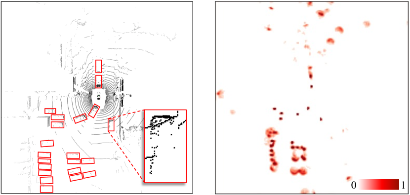
Figure 1: Visualization of input and heatmaps of CenterPoint in BEV for $Car$. Most values in the heatmaps are nearly zero, while the dense head computes over all BEV features, which is wasteful.

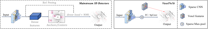
Figure 2: Pipelines of mainstream 3D object detectors and VoxelNeXt. These 3D detectors [57, 41, 12] rely on sparse-to-dense conversion, anchors/centers, and dense heads with NMS. RoI pooling is an option for two-stage detectors [12, 41]. In contrast, VoxelNeXt is a fully sparse convolutional network, which predicts results directly upon voxel features, with either fully connected layers or sparse convolutions.

In Fig. 1, we visualize the heatmap in CenterPoint [57]. It is clear that a large portion of space has nearly zero prediction scores. Due to inherent sparsity and many background points, only a small number of points have responses, i.e., less than 1% for Car class on average of nuScenes validation set. However, the dense prediction head computes over all positions in the feature map, as required by the dense convolution computation. They not only waste much computation, but also complicate detection pipelines with redundant predictions. It requires to use non-maximum suppression (NMS) like post-processing to remove duplicate detections, preventing the detector from being elegant. These limitations motivate us to seek alternative sparse detection solutions.

In this paper, we instead propose VoxelNeXt. It is a simple, efficient, and post-processing-free 3D object detector. The core of our design is a voxel-to-object scheme, which directly predicts 3D objects from voxel features, with a strong fully sparse convolutional network. The key advantage is that our approach can get rid of anchor proxies, sparse-to-dense conversion, region proposal networks, and other complicate components. We illustrates the pipelines of mainstream 3D detectors and ours in Fig. 2.

High inference efficiency is due to our voxel-to-object scheme avoiding dense feature maps. It predicts only upon sparse and necessary locations, as listed in Tab. 1 with comparison to CenterPoint [57]. This representation also makes VoxelNeXt easily extended to 3D tracking with an offline tracker. Previous work [57] only tracks for the predicted object centers, which might involve prediction bias to its positions. In VoxelNeXt, the query voxels, i.e., the voxels for box prediction, can also be tracked for association.

Recently, FSD [16] exploits the fully sparse framework. Motivated by VoteNet [37], it votes for object centers and resorts to iterative refinement. Since 3D sparse data is generally scattered on object surfaces, this voting process inevitably introduces bias or error. Consequently, refinement, such as iterative group correction, is needed to ensure final accuracy. The system is complicated by its heavy belief in object centers. FSD [16] is promising at the large-range Argoverse2, while its efficiency is inferior to ours, as in Fig. 3.

To demonstrate the effectiveness of VoxelNeXt, we evaluate our models on three large-scale benchmarks of nuScenes [3], Waymo [45], Argoverse2 [52] datasets. VoxelNeXt achieves leading performance with high efficiency on 3D object detection on both these benchmarks. It also yields state-of-the-art performance on 3D tracking. Without bells and whistles, it ranks 1^st among all LIDAR-only entries on the nuScenes tracking test split [3].

2 Related Work

LIDAR Detectors 3D detectors usually work similar to their 2D counterparts, such as R-CNN series [12, 34, 41, 54] and CenterPoint series [57, 14, 60]. 3D detection distinguishes from the 2D task due to the sparsity of data distribution. But many approaches [61, 53, 57, 12] still seek 2D dense convolutional heads as a solution.

Table 1: Comparison with CenterPoint on nuScenes dataset. VoxelNeXt presents better performance with high efficiency.

Method	mAP	NDS	FLOPs
			Sparse CNN	Head
CenterPoint [57]	58.6	66.2	62.9 G	123.7 G
VoxelNeXt	60.0	67.1	33.6 G	5.1 G

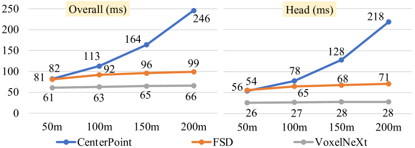
Figure 3: Latency on Argoverse2 and various perception ranges.

VoxelNet [61] uses PointNet [38] for voxel feature encoding and then applies dense region proposal network and head for prediction. SECOND [53] improves VoxelNet by efficient sparse convolutions with the dense anchor-based head. Other state-of-the-art methods, including PV-RCNN [41], Voxel R-CNN [12], and VoTr [35], still keep the sparse-to-dense scheme to enlarge the receptive field.

Motivated by 2D CenterNet [14], CenterPoint [57] is applied to 3D detection and tracking. It converts the sparse output of a backbone network into a map-view dense feature map and predicts a dense heatmap of the center locations of objects, based on the dense feature. This dense center-based prediction has been adopted by several dense-head approaches [33, 30]. In this paper, we take a new direction and surprisingly show that a simple and strong sparse CNN is sufficient for direct prediction. The notable finding is that the dense head is not always necessary.

Sparse Detectors Methods of [16, 47, 46] avoid dense detection heads and instead introduce other complicated pipelines. RSN [47] performs foreground segmentation on range images and then detects 3D objects on the remained sparse data. SWFormer [46] proposes a sparse transformer with delicate window splitting and multiple heads with feature pyramids. Motivated by VoteNet [37], FSD [16] use point clustering and group correction to solve the issue of center feature missing. These detectors conduct sparse prediction, but complicate detection pipelines in different ways. In our work, this center-missing issue can also be simply skipped through sparse networks that have large receptive fields. We make minimal adaptations to commonly-used sparse CNNs to realize fully sparse detectors.

Sparse Convolutional Networks Sparse CNNs become mainframe backbone networks in 3D deep learning [41, 10, 11, 23] for its efficiency. It is common wisdom that its representation ability is limited for prediction. To remedy it, 3D detectors of [53, 41, 12, 49] rely on dense convolutional heads for feature enhancement. Recent methods [6, 32] make convolutional modifications upon sparse CNNs. Approaches of [35, 21] even substitute it with transformers for large receptive fields. Contrary to all these solutions, we demonstrate that the insufficient receptive field bottleneck can be simply addressed by additional down-sampling layers without any other complicated design.

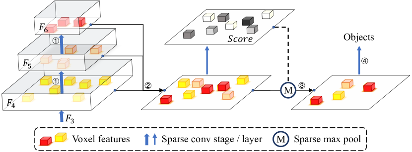
Figure 4: Detailed structure of VoxelNeXt framework. Circled numbers in the figure correspond to the paragraphs in Sections 3.1 and 3.2. 1 - Additional down-samplings. 2 - Sparse height compression. 3 - Voxel selection. 4 - Box regression. We omit the generation of $F_{1}$, $F_{2}$, and $F_{3}$ here for the simplicity sake.

3D Object Tracking 3D object tracking models tracklets of multiple objects along multi-frame LIDAR. Most previous methods [9, 2, 51] directly use the Kalman filter upon detection results, such as AB3DMOT [51]. CenterPoint [57] predicts the velocities to associate object centers through multiple frames, following CenterTrack [60]. In this paper, we include query voxels for association, which effectively relieve the prediction bias of object centers.

3 Fully Sparse Voxel-based Network

Point clouds or voxels are irregularly distributed and usually scattered at the surface of 3D objects, not at the center or inside. This motivates us to study along a new direction to predict 3D boxes directly based on the voxels instead of the hand-crafted anchors or centers.

To this end, we aim for minimal modification to adapt a plain 3D sparse CNN network to the direct-voxel prediction. In the following, we introduce the backbone adaptation (Section 3.1), the sparse head design (Section 3.2), and the extension to 3D object tracking (Section 3.3).

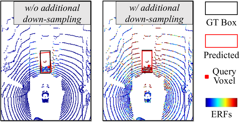
Figure 5: Effects of additional down-sampling layers on effective receptive fields (ERFs) and the predicted boxes.

3.1 Sparse CNN Backbone Adaptation

Additional Down-sampling Strong feature representation with sufficient receptive fields is a must to ensure direct and correct prediction upon sparse voxel features. Although the plain sparse CNN backbone network has been widely used in 3D object detectors [41, 12, 57], recent work presents its weakness and proposes various methods to enhance the sparse backbone using, e.g., well-designed convolution [7], large kernels [8], and transformers [35, 26, 25].

Unlike all these approaches, we make as little as possible modification to accomplish this, only using additional down-sampling layers. By default, the plain sparse CNN backbone network has 4 stages, with the feature strides {1, 2, 4, 8}. We name the output sparse features {$F_{1},F_{2},F_{3},F_{4}$} respectively. This setting is incapable of direct prediction, especially for large objects. To enhance its ability, we simply include two additional down-sampling layers to obtain features with strides {16, 32} for {$F_{5},F_{6}$}. This small change directly imposes notable effects to enlarge receptive fields. We combine the sparse features from the last three stages {$F_{4},F_{5},F_{6}$} to $F_{c}$. Their spatial resolutions are all aligned to $F_{4}$. For stage $i$, $F_{i}$ is a set of individual features $f_{p}$. $p\in P_{i}$ is a position in 3D space, with the coordinate ($x_{p}$, $y_{p}$, $z_{p}$). This process is shown in Fig. 4. It is noteworthy that this simple sparse concatenation requires no other parameterized layers. Sparse features $F_{c}$ and their positions $P_{c}$ are obtained as

$${F}_{c}=F_{4}\cup(F_{5}\cup F_{6}),\qquad$$ (1)

$$P_{6}^{\prime}=\{(x_{p}\times 2^{2},\,y_{p}\times 2^{2},\,z_{p}\times 2^{2})\,|\,p\in P_{6}\}$$

$$P_{5}^{\prime}=\{(x_{p}\times 2^{1},\,y_{p}\times 2^{1},\,z_{p}\times 2^{1})\,|\,p\in P_{5}\}$$

$${P}_{c}=P_{4}\cup(P_{5}^{\prime}\cup P_{6}^{\prime}).\qquad$$

We visualize the effective receptive fields (ERFs) in Fig. 5. With additional down-sampling layers, ERFs are larger and the predicted box is more accurate. It is effective enough and costs little extra computation, as in Tab. 2. Thus, we use this simple design as the backbone network.

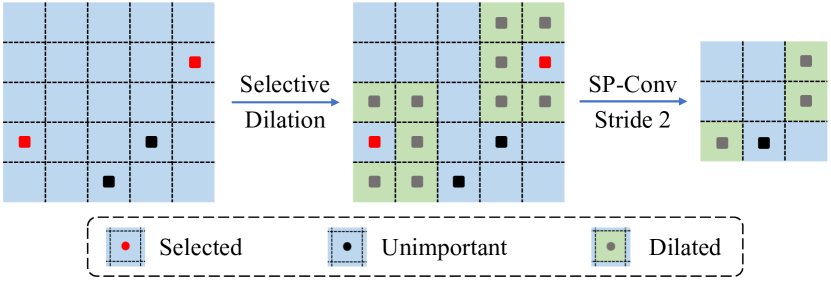
Figure 6: Spatially voxel pruning. In sparse CNN backbone, down-sampling layers commonly dilate all voxels to the kernel shape, before down-sampling. Different from these approaches, we only dilate selected voxels that have high feature magnitudes to maintain high efficiency.

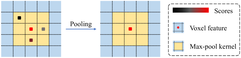
Figure 7: Sparse max pooling layer. Similarly to submanifold sparse convolution [19], it only operates on non-empty positions. It removes non-maximum voxels in local space.

Sparse Height Compression 3D object detectors of [57, 41, 12] compress 3D voxel features into dense 2D maps by converting sparse features to dense ones and then combining depth (along $z$ axis) into the channel dimension. These operations cost footprint memory and computation.

In VoxelNet, we find that 2D sparse features are efficient for prediction. Height compression in VoxelNeXt is fully sparse. We simply put all voxels onto the ground and sum up features in the same positions. It costs no more than 1ms. We find that prediction upon the compressed 2D sparse features cost less than using 3D ones, as shown in Tab. 5.The compressed sparse features $\bar{F_{c}}$ and their positions $\bar{P_{c}}$ are obtained as:

$$\bar{P_{c}}=\{(x_{p},\,y_{p})\,|\,p\in P_{c}\}$$ (2)

$$\bar{F_{c}}=\{\sum_{p\in S_{\bar{p}}}f_{p},|\,\bar{p}\in\bar{P_{c}}\}$$

where $S_{\bar{p}}=\{p\,|\,x_{p}=x_{\bar{p}},\,y_{p}=y_{\bar{p}},\,p\in P_{c}\}$, containing voxels that are put onto the same 2D position $\bar{p}$.

Spatially Voxel Pruning Our network is completely based on voxels. It is common that 3D scenes contain a large number of background points that is redundant and have little benefit for prediction. We gradually prune irrelevant voxels along down-sampling layers. Following SPS-Conv [32], we suppress the dilation of voxels with small feature magnitudes, as shown in Fig. 6. Taking the suppression ratio as 0.5, we only dilate the voxels whose feature magnitudes $|f_{p}|$ (averaged on the channel dimension) rank top half of all voxels. The voxel pruning largely saves computation without compromising performance as indicated in Tab. 3.

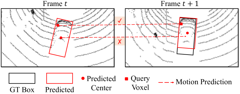
Figure 8: Visualization of voxel association. The predicted object centers are conventionally used for tracking. We additionally associate query voxels in case that the predicted centers are inaccurate.

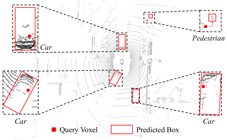
Figure 9: Visualization on the predicted boxes and their query voxels. For the Car objects, query voxels are inside and usually near the boundaries. For the pedestrian consisting of limited voxels, its query voxel is outside. More visualizations are in the appendix.

3.2 Sparse Prediction Head

Voxel Selection Figure 4 shows the detailed framework of the VoxelNeXt model. Instead of relying on the dense feature map $\mathbf{M}$, we directly predict objects based on the sparse output of the 3D CNN backbone network $\mathbf{V}\in\mathbb{R}^{N\times F}$. We first predict the scores of voxels for $K$ classes, $\mathbf{s}\in\mathbb{R}^{N\times K}$. During training, we assign the voxel nearest to each annotated bounding box center as a positive sample. We use a focal loss [31] for supervision. We note the fact that during inference query voxels are commonly not at the object center. They are even not necessarily inside the bounding boxes, e.g., for pedestrian in Fig. 9. We count the distribution of query voxels in Tab. 7 on nuScenes validation set.

Table 2: Results of a pilot study on nuScenes validation split, for the strides of fully sparse voxel-based prediction. Latency is evaluated on a single GPU. For $D_{3}$, the arrows indicate the change based on CenterPoint. For others, the arrows indicate the change based on $D_{3}$.

Method	Strides	Latency	mAP	NDS	Car	Truck	Bus	Trailer	C.V.	Ped	Mot	Byc	T.C.	Bar
CenterPoint	{2, 4, 8}	96 ms	55.6	63.2	83.5	54.9	67.5	30.6	16.3	83.3	52.7	34.5	65.6	66.5
$D_{3}$	{2, 4, 8}	56 ms	46.7↓8.9	56.2	75.3	41.3	38.3	10.5	14.9	82.0	47.7	28.3	63.6	64.2
$D_{3}^{5\times 5\times 5}$	{2, 4, 8}	225 ms	51.6↑4.9	60.4	80.0	49.2	56.8	16.8	16.5	83.5	50.2	30.9	64.8	67.7
$D_{4}$	{2, 4, 8, 16}	62 ms	52.3↑5.6	61.2	80.0	50.0	61.2	23.1	16.9	82.5	49.0	31.8	63.9	64.8
$D_{5}$	{2, 4, 8, 16, 32}	66 ms	56.5↑9.5	64.5	83.0	54.0	67.4	32.9	20.0	84.1	52.7	35.7	66.6	65.3

Table 3: Effects of spatial pruning ratios. A larger pruning ratio means that fewer voxels remain in the sparse CNN backbone.

Ratio	-	0.1	0.3	0.5	0.7	0.9
FLOPs (G)	83.8	79.6	60.1	33.6	19.8	7.6
mAP	56.5	56.5	56.4	56.2	53.7	45.1
NDS	64.5	64.5	64.3	64.3	62.1	56.0

Table 4: Effects of spatial pruning on various layers. We use it on the first 3 down-sampling layers by default.

Stages	-	1	2	3	4	5
FLOPs (G)	83.8	65.0	45.9	33.6	29.1	27.9
mAP	56.5	56.5	56.4	56.2	54.2	53.7
NDS	64.5	64.5	64.4	64.3	62.5	62.0

During inference, we avoid NMS post-processing by using sparse max pooling, as features are sparse enough. Similar to submanifold sparse convolution [19], it only operates on non-empty positions. This is based on the predicted scores $\mathbf{s}$ and conducted individually for each class. We adopt sparse max pooling to select voxels with spatially local maximums. The removed voxels will be excluded in box prediction, which saves the computation of head.

Box Regression Bounding boxes are directly regressed from the positive or selected sparse voxel features $\mathbf{v}\in\mathbb{R}^{n\times F}$. Following the protocol in CenterPoint [57], we regress the location $(\Delta x,\Delta y)\in\mathbb{R}^{2}$, height $h\in\mathbb{R}$, 3D size $s\in\mathbb{R}^{3}$, and rotation angle $(sin(\alpha),cos(\alpha))\in\mathbb{R}^{2}$. For the nuScenes dataset or tracking, we regress the velocity $v\in\mathbb{R}^{2}$ by task definition. These predictions are supervised under the L1 loss function during training. For Waymo dataset, we also predict the IoU and train with IoU loss for performance enhancement [22]. We simply use fully connected layer or $3\times 3$ submanifold sparse convolutional layers with kernel size 3 for prediction, without other complicate designs. We find that the $3\times 3$ sparse convolutions generate better results than fully connected layers, with limited burden, as in Tab. 6.

3.3 3D Tracking

Our framework is naturally extended to 3D tracking. CenterPoint [57] tracks the predicted object centers via a two-dimensional velocity $v\in\mathbb{R}^{2}$, which is also supervised by L1 loss. We extend this design into VoxelNeXt. Our solution is to use voxel association to include more tracklets that match the positions of query voxels.

As shown in Fig. 8, we record the position of voxel that is used to predict each box. Similar to the center association, we compute the L2 distance for matching. The query positions are picked by tracking back their index to original input voxels, instead of stride-8 positions. The tracked voxels exist in input data, which has less bias than the predicted centers. Also, the query voxels between adjacent frames share similar relative positions to boxes. We empirically show that voxel association improves tracking in Tab. 11.

4 Experiments

Table 5: Ablations on 2D or 3D sparse CNN in VoxelNeXt. sparse height Compression is used to connect 3D backbone and 2D head.

Method	Backbone	Head	Latency	mAP	NDS
-	3D	3D	92 ms	56.3	63.4
VoxelNeXt	3D	2D	66 ms	56.2	64.3
VoxelNeXt-2D	2D	2D	61 ms	53.4	62.6

Table 6: Effects of the layer type in the sparse prediction head. $1\times 1$ submanifold sparse convolution [19] is the fully connected.

Head kernel size	Head latency	mAP	NDS
$1\times 1$ (FC)	30 ms	56.2	64.3
$3\times 3$ (SpConv)	35 ms	56.8	64.5

Table 7: Ratios of relative positions of query voxels to the boxes predicted from them. We only take high-quality predicted boxes (IoU with ground-truth boxes $>$ 0.7 and with matched predicted labels) into consideration. According to the relative positions to their predicted boxes, we split voxels into 3 types of near center, near boundary, and outside box. Overall, most voxels are inside but not near center.

Class	Mean	Car	Truck	Bus	Trailer	C.V.	Ped	Mot	Byc	T.C.	Bar
Near center	9.9%	10.3%	5.6%	15.2%	1.2%	16.3%	12.5%	19.6%	13.1%	10.8%	17.8%
Near boundary	72.8%	84.3%	39.2%	58.8%	84.6%	51.8%	42.3%	66.5%	54.7%	39.7%	58.7%
Outside box	17.3%	5.4%	55.3%	26.0%	14.2%	31.9%	45.2%	13.9%	32.2%	49.6%	23.5%

Table 8: Comparison to the representative dense-head method Centerpoint [57]. ATE, ASE, AOE, AVE, and AAE denote the errors of location, size, orientation, velocity, and attribute.

Method	mAP	NDS	ATE	ASE	AOE	AVE	AAE
CenterPoint	55.6	63.5	29.7	25.7	44.5	24.5	18.8
VoxelNeXt	56.5	64.5	29.9	25.4	39.6	23.2	19.0
	$\uparrow$0.9	$\uparrow$1.0	$\uparrow$0.2	$\downarrow$0.3	$\downarrow$4.9	$\downarrow$1.3	$\uparrow$0.2

Table 9: Efficiency statistics on sparse CNN backbone. The computations of Stage 5&6 are limited by their small voxel numbers.

Stage	1	2	3	4	5	6
Channel	16	32	64	128	128	128
Voxels (K)	82.6	46.7	18.2	6.4	3.0	1.3
FLOPs (G)	1.1	4.7	8.2	11.7	6.1	2.8
Latency (ms)	4	5	6	7	6	3

Table 10: Effects of sparse max-pool and NMS post-processing. The max-pool follows the submanifold sparse convolution pattern.

Max-pool	NMS	mAP	NDS
✗	✗	33.0	51.0
✗	✓	56.0	64.2
✓	✗	56.2	64.3
✓	✓	56.2	63.3

Table 11: Voxel association on nuScenes tracking validation set.

+ Voxel association	AMOTA	AMOTP	MOTA	IDS
✗	69.1	61.6	59.3	643
✓	70.2	64.0	61.5	729

Table 12: Performance of 3D object detection methods on nuScenes test set. ^† means the method that uses double-flip testing. All models listed take LIDAR data as input without image fusion or any model ensemble.

Method	mAP	NDS	Latency	Car	Truck	Bus	Trailer	C.V.	Ped	Mot	Byc	T.C.	Bar
PointPillars [27]	30.5	45.3	31 ms	68.4	23.0	28.2	23.4	4.1	59.7	27.4	1.1	30.8	38.9
3DSSD [55]	42.6	56.4	-	81.2	47.2	61.4	30.5	12.6	70.2	36.0	8.6	31.1	47.9
CBGS [62]	52.8	63.3	80 ms	81.1	48.5	54.9	42.9	10.5	80.1	51.5	22.3	70.9	65.7
CenterPoint [57]	58.0	65.5	96 ms	84.6	51.0	60.2	53.2	17.5	83.4	53.7	28.7	76.7	70.9
CVCNET [4]	58.2	66.6	122 ms	82.6	49.5	59.4	51.1	16.2	83.0	61.8	38.8	69.7	69.7
HotSpotNet [5]	59.3	66.0	-	83.1	50.9	56.4	53.3	23.0	81.3	63.5	36.6	73.0	71.6
AFDetV2 [22]	62.4	68.5	-	86.3	54.2	62.5	58.9	26.7	85.8	63.8	34.3	80.1	71.0
Focals Conv [7]	63.8	70.0	138 ms	86.7	56.3	67.7	59.5	23.8	87.5	64.5	36.3	81.4	74.1
VISTA [13]†	63.0	69.8	94 ms	84.4	55.1	63.7	54.2	25.1	82.8	70.0	45.4	78.5	71.4
UVTR-L [28]†	63.9	69.7	132 ms	86.3	52.2	62.8	59.7	33.7	84.5	68.8	41.1	74.7	74.9
PillarNet-18 [40]†	65.0	70.8	78 ms	87.4	56.7	60.9	61.8	30.4	87.2	67.4	40.3	82.1	76.0
VoxelNeXt-2D	64.1	69.8	61 ms	84.8	52.7	62.3	56.2	29.5	84.5	72.5	45.7	78.8	73.7
VoxelNeXt	64.5	70.0	66 ms	84.6	53.0	64.7	55.8	28.7	85.8	73.2	45.7	79.0	74.6
VoxelNeXt†	66.2	71.4	-	85.3	55.7	66.2	57.2	29.8	86.5	75.2	48.8	80.7	76.1

Table 13: Performance of nuScenes 3D tracking test split for LIDAR-only methods, without multi-modal extension. ^† is based on the double-flip 3D object detection results in Tab. 12.

Method	AMOTA	AMOTP	MOTA	IDS
AB3DMOT [51]	15.1	150.1	15.4	9027
CenterPoint [57]	63.8	55.5	53.7	760
CBMOT [2]	64.9	59.2	54.5	557
OGR3MOT [58]	65.6	62.0	55.4	288
SimpleTrack [36]	66.8	55.0	56.6	575
UVTR-L [28]	67.0	55.0	56.6	774
TransFusion-L [1]	68.6	52.9	57.1	893
VoxelNeXt	69.5	56.8	58.6	785
VoxelNeXt†	71.0	51.1	60.0	654

4.1 Ablation Studies

Additional Down-sampling Layers We ablate the effect of the down-sampling layers in VoxelNeXt. We extend it to the variants $D_{s}$. $s$ denotes the number of down-sampling. For example, $D_{3}$ has the same network strides (3 times) to the base model. Our modification does not change the resolution for the detection head. The results of these models are shown in Tab. 2. Without the dense head, $D_{3}$ suffers from serious performance drop, especially on large objects of Truck and Bus. From $D_{3}$ to $D_{5}$, performance gradually increases. Additional down-sampling layers compensate for the receptive field. To verify this, we add one more variant, $D_{3}^{5\times 5\times 5}$, which increases the kernel size of sparse convolutions in all stages to $5\times 5\times 5$. Large kernel improves the performance to some extend but degrades efficiency. Thus, we use additional down-samplings as a simple solution.

Table 14: Performance of nuScenes 3D tracking validation set. All methods listed are LIDAR-only, without multi-modal extension.

Method	AMOTA	AMOTP	MOTA	IDS
AB3DMOT [51]	57.8	80.7	51.4	1275
MPN-Baseline	59.3	83.2	51.4	1079
CenterPoint [57]	66.5	56.7	56.2	562
CBMOT [2]	67.5	59.1	58.3	494
OGR3MOT [48]	69.3	62.7	60.2	262
SimpleTrack [36]	69.6	54.7	60.2	405
VoxelNeXt	70.2	64.0	61.5	729

Table 15: Performance of 3D object detection results on the Waymo validation split. Results with the instance-decreasing trick in the ground-truth sampling [16] is in the appendix. All models take single-frame data as input without test-time augmentations or ensemble.

Method	mAP/mAPH	Vehicle		Pedestrian		Cyclist
	L2	L1 AP/APH	L2 AP/APH	L1 AP/APH	L2 AP/APH	L1 AP/APH	L2 AP/APH
Pillar-OD [50]	-	69.8 / -	- / -	72.5 / -	-	-	-
VoxSeT [21]	-	76.0 / -	68.2 / -	-	-	-	-
VoTr-TSD [35]	-	74.9 / 74.3	65.9 / 65.3	-	-	-	-
SECOND [53]	61.0 / 57.2	72.3 / 71.7	63.9 / 63.3	68.7 / 58.2	60.7 / 51.3	60.6 / 59.3	58.3 / 57.0
M3METR [20]	61.8 / 58.7	75.7 / 75.1	66.0 / 66.0	65.0 / 56.4	56.0 / 48.4	65.4 / 64.2	62.7 / 61.5
IA-SSD [59]	62.3 / 58.1	70.5 / 69.7	61.6 / 61.0	69.4 / 58.5	60.3 / 50.7	67.7 / 65.3	65.0 / 62.7
PointPillars [27]	62.8 / 57.8	72.1 / 71.5	63.6 / 63.1	70.6 / 56.7	62.8 / 50.3	64.4 / 62.3	61.9 / 59.9
RangeDet [17]	65.0 / 63.2	72.9 / 72.3	64.0 / 63.6	75.9 / 71.9	67.6 / 63.9	65.7 / 64.4	63.3 / 62.1
3D-MAN [56]	-	74.5 / 74.0	67.6 / 67.1	71.7 / 67.7	62.6 / 59.0	-	-
LIDAR-RCNN [29]	65.8 / 61.3	76.0 / 75.5	68.3 / 67.9	71.2 / 58.7	63.1 / 51.7	68.6 / 66.9	66.1 / 64.4
PV-RCNN [41]	66.8 / 63.3	77.5 / 76.9	69.0 / 68.4	75.0 / 65.6	66.0 / 57.6	67.8 / 66.4	65.4 / 64.0
Part-A2-Net [44]	66.9 / 63.8	77.1 / 76.5	68.5 / 68.0	75.2 / 66.9	66.2 / 58.6	68.6 / 67.4	66.1 / 64.9
SST [15]	67.8 / 64.6	74.2 / 73.8	65.5 / 65.1	78.7 / 69.6	70.0 / 61.7	70.7 / 69.6	68.0 / 66.9
PV-RCNN++ [42]	68.4 / 64.9	78.8 / 78.2	70.3 / 69.7	76.7 / 67.2	68.5 / 59.7	69.0 / 67.6	66.5 / 65.2
CenterPoint [57]	69.8 / 67.6	76.6 / 76.0	68.9 / 68.4	79.0 / 73.4	71.0 / 65.8	72.1 / 71.0	69.5 / 68.5
AFDetV2 [22]	71.0 / 68.8	77.6 / 77.1	69.7 / 69.2	80.2 / 74.6	72.2 / 67.0	73.7 / 72.7	71.0 / 70.1
PillarNet-34 [40]	71.0 / 68.5	79.1 / 78.6	70.9 / 70.5	80.6 / 74.0	72.3 / 66.2	72.3 / 71.2	69.7 / 68.7
SWFormer [46]	-	77.8 / 77.3	69.2 / 68.8	80.9 / 72.7	72.5 / 64.9	-	-
FSDspconv [16]	71.9 / 69.7	77.8 / 77.3	68.9 / 68.5	81.9 / 76.4	73.2 / 68.0	76.5 / 75.2	73.8 / 72.5
VoxelNeXt-2D	70.9 / 68.2	77.9 / 77.5	69.7 / 69.2	80.2 / 73.5	72.2 / 65.9	73.3 / 72.2	70.7 / 69.6
VoxelNeXtK3	72.2 / 70.1	78.2 / 77.7	69.9 / 69.4	81.5 / 76.3	73.5 / 68.6	76.1 / 74.9	73.3 / 72.2

Table 16: Performance of 3D object detection results Argoverse2 dataset.

Methods	mAP	Veh.	Bus	Ped.	Stop.	Box.	Boll.	C-B.	M.-list	MPC.	M.-cycle	Bicycle	A-B.	School.	Truck.	C-C.	V-T.	Sign	Large.	Str.	Bic.-list
CenterPoint [57]	22.0	67.6	38.9	46.5	16.9	37.4	40.1	32.2	28.6	27.4	33.4	24.5	8.7	25.8	22.6	29.5	22.4	6.3	3.9	0.5	20.1
FSD	28.2	68.1	40.9	59.0	29.0	38.5	41.8	42.6	39.7	26.2	49.0	38.6	20.4	30.5	14.8	41.2	26.9	11.9	5.9	13.8	33.4
VoxelNeXt	30.0	71.7	39.2	63.1	39.2	40.0	52.5	63.7	42.2	34.9	42.7	40.1	20.1	25.2	16.9	45.7	22.3	15.8	5.9	9.8	33.5
VoxelNeXtK3	30.7	72.7	38.8	63.2	40.2	40.1	53.9	64.9	44.7	39.4	42.4	40.6	20.1	25.2	19.9	44.9	20.9	14.9	6.8	15.7	32.4

Spatially Voxel Pruning VoxelNeXt gradually drops redundant voxels according to feature magnitude. We ablate this setting in Tab. 3. We control the drop ratio from 0.1 to 0.9 with an interval of 0.2. The performance hardly decays when the ratio is not greater than 0.5. Thus, we set the drop ratio to 0.5 as a default setting in our experiments. We also ablate the stages of voxel pruning in Tab. 4. We use it on the first 3 stages by default.

Sparse Height Compression We make ablations on the sparse CNN types of 2D and 3D, in the backbone and head of VoxelNeXt, in Tab. 5. The naive design is that both the backbone and head apply 3D sparse CNN, which results in high latency. With the sparse height compression, we combine the 3D backbone and 2D sparse prediction head. It achieves much better efficiency with decent performance. We use it as a default setting of VoxelNeXt. When we use 2D sparse CNN as the backbone network, it has the same layer number and double channels as the 3D one. It achieves the best efficiency, and yet suffers a bit of performance drop. We name it VoxelNeXt-2D for its high efficiency.

Layer Type in Sparse Prediction Head We ablate the effect using fully-connected layers or submanifold sparse convolutions to predict boxes in the sparse head, as shown in Tab. 6. The fully-connected (FC) head has inferior performance to the $3\times 3$ sparse convolution counterpart, but more efficient. We denote the latter with $K3$ in VoxelNeXt.

Relative Positions between Voxels and Predicted Boxes In VoxelNeXt, voxels for box prediction are not required to be inside the boxes, not to mention centers, as in Tab. 7. We count the relative of voxels that are inside the 3D bounding boxes they generate. We split voxels into 3 area types of near center, near boundary, and outside box, according to their relative positions to boxes. On average, most boxes are predicted from voxels inside, maybe not near centers. Statistically, only a few boxes (less than 10% in total) are predicted based on the voxels near object centers. This finding shows that boundary voxels are also qualified for prediction, while object centers are not always necessary.

Another observation is that there are large gaps between the ratios of different classes. For Car and Trailer, most boxes are predicted on inside voxels. In contrast, for Truck, Traffic Cone, and Pedestrian, about half of the boxes are predicted from outside voxels. We illustrate example pairs in Fig. 9. As objects in different classes vary in size and spatial sparsity, predicting upon voxels complies with data distribution, rather than proxies like anchors or centers.

Comparison to CenterPoint in Error Analysis We compare VoxelNeXt to the representative dense-head method CenterPoint [57] in Tab. 8. Training on 1/4 nuScenes training set and evaluating on the full validation split, VoxelNeXt achieves 0.9% mAP and 1.0% NDS improvement. In further analysis, CenterPoint and VoxelNeXt shares comparable errors in location, size, and velocity. However, there are large gaps in other error types, especially in orientation. Notably, VoxelNext has 4.9% less orientation error than CenterPoint. We suppose that this results from that sparse voxel features might be more sensitive to orientation difference.

Efficiency Statistics of Backbone We count the efficiency-related statistics of our sparse CNN backbone network in Tab. 9. As features in the last 3 stages are summed up for height compression, they share the same channel number 128. Due to the high down-sampling ratios in Stages 5-6, their voxel numbers are much smaller compared to previous stages. Consequently, the computation cost introduced in Stages 5-6 is limited to 6.1G and 2.8G FLOPs in 6 and 3 ms. It is no more than $1/3$ of the overall backbone network, and yet makes notable effects on performance enhancement.

Sparse Max Pooling We ablate the effect of sparse max pooling and NMS in Tab. 10. Compared to the commonly used NMS, max-pool presents comparable mAP, 56.0% v.s. 56.2%. VoxelNeXt is flexible to works either with NMS or sparse max pooling. Max-pool is an elegant solution and avoids some unnecessary computation on predictions.

Voxel Association for 3D Tracking Tab. 11 shows the ablation of 3D tracking on nuScenes validation. In addition to tracking predicted box centers, we also include the voxels that predict boxes for matching. Voxel association introduces notable improvement of 1.1% AMOTA.

4.2 Main Results

3D Object Detection In Tab. 12, we evaluate our detection models on the test split and compare them with other LIDAR-based methods on nuScenes test set. Results denoted as $\dagger$ [13, 28, 40] are reported with the double-flip testing augmentation [57]. Both lines of results are better than previous ones. We compare VoxelNeXt with other 3D object detectors on the Waymo validation split in Tab. 15 and on Argoverse2 [52] in Tab. 16. We present latency comparison in Tab. 12 and Fig. 3. VoxelNeXt achieves leading performance among these methods with high efficiency.

3D Multi-object Tracking In Tab. 13 and Tab. 14, we compare VoxelNeXt’s tracking performance with other methods in the nuScenes test and validation splits. VoxelNeXt achieves the best AMOTA among all LIDAR-based methods. In addition, when combined with the double-flip testing results in Tab. 12, denoted as ^† in Tab. 13, VoxelNeXt further achieves 71.0% AMOTA and ranking 1^st on the nuScenes 3D LIDAR tracking benchmark.

5 Conclusion and Discussion

In this paper, we have presented a fully sparse and voxel-based framework for 3D object detection and tracking. It is with simple techniques, run fast with no much extra cost, and works in an elegant manner without NMS post-processing. For the first time, we show that direct voxel-based prediction is feasible and effective. Thus rule-based schemes, e.g., anchors or centers, and dense heads become unnecessary in ours. VoxelNeXt presents promising results on large-scale datasets, including nuScenes [3], Waymo [45], and Argoverse2 [52]. With high efficiency, it achieves leading performance on 3D object detection and ranks 1_st on nuScenes 3D tracking LIDAR benchmark.

Limitations A gap exists between theoretical FLOPs and actual inference speed. VoxelNeXt has a much small 38.7G FLOPs, compared to 186.6G of CenterPoint [57]. The actual latency reduction is clear but not so large as FLOPs in Tab. 1, as it highly depends on implementation and devices.

Appendix

In this appendix, we first introduce implementation details in Sec. A. We then include additional experimental results in Sec. B. We also provide more visualizations and discussions in Sec. C and Sec. D.

Appendix A Implementation Details

nuScenes [3] has 1,000 drive sequences, split into 700, 150, and 150 sequences for training, validation, and testing. nuScenes is collected by a 32-beam synced LIDAR and 6 cameras. The annotations include 10 classes. In the ablation study, detection models are trained on 1/4 training data and evaluated on the full validation set.

Waymo [45] is a large-scale public autonomous driving dataset, which contains 1,150 sequences in total, with 798 for training, and 202 for validation. It was collected by one long-range LiDAR sensor at 75 meters and four near-range sensors.

Argoverse2 [52] has 1000 sequences, including 700 for training, 150 for validation. The perception range is 200 radius meters, covering area of 400m × 400m. We follow FSD [16] for data processing.

Voxelization

For nuScenes [3] dataset, point clouds are clipped in [-54m, 54m] for X or Y axis, and [-5m, 3m] for Z axis. Voxel size is (0.075m, 0.075m, 0.2m) by default. For VoxelNeXt-2D, the voxel size along Z axis is 8m.

For Waymo [45] dataset, point clouds are clipped into [-75.2m, 75.2m] X or Y axis, and [-2m, 4m] for Z axis. Voxel size is (0.1m, 0.1m, 0.15m) by default. For VoxelNeXt-2D, the voxel size along Z axis is 6m.

For Argoverse2 [52] dataset, we use (0.1m, 0.1m, 0.2m) as voxel size. The perception range is [-200m, 200m] for X or Y axis. The range for Z is [-20m, 20m].

Data Augmentations

For nuScenes dataset, random flipping, global scaling, global rotation, GT sampling [53], and translation augmentations are used. Flipping is randomly conducted along X and Y axes. Rotation angle is randomly picked between -45^o and 45^o. Global scaling is conducted by a factor sampled between 0.9 and 1.1. The translation noise factors are sampled between 0 and 0.5. Only for test submission models, GT sampling is removed in the last 5 training epochs [28].

For Waymo dataset, data augmentations also include random flipping, global scaling, global rotation, and ground-truth (GT) sampling [53]. These settings are similar to those of nuScenes dataset and follow baseline methods [57, 41].

For Argoverse2 dataset, we use similar data augmentation to nuScenes and Waymo, except that we do not use ground-truth sampling.

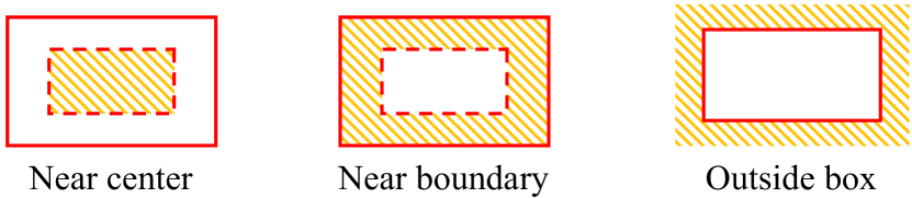
Figure 10: The relative positions of query voxel to the predicted boxes, e.g., near center, near boundary, outside box, corresponding to Tab. 7 in the paper.

Training Hyper-parameters

For nuScenes dataset, models are trained for 20 epochs with batch size 16. They are optimized with Adam [24]. Learning rate is initially 1e-3 and decays to 1e-4 in a cosine annealing. Weight decay is 0.01. Gradients are clipped by norm 35. These settings follow CenterPoint [57].

For Waymo dataset, models are trained for 12 epochs by default. Batch size is set as 16. Learning rate is initialized as 3e-3. They are also optimized with Adam [24].

For Argoverse2 dataset, we use similar settings to Waymo, except that only 6 epochs for training is enough.

Table 17: Comparison on the nuScenes validation split. This table presents detailed performance for Tab. 1 in the paper.

Method	mAP	NDS	Car	Truck	Bus	Trailer	C.V.	Ped	Mot	Byc	T.C.	Bar
SECOND [53]	50.6	62.3	81.8	51.7	66.9	37.3	15.0	77.7	42.5	17.5	57.4	59.2
CenterPoint [57]	58.6	66.2	85.0	58.2	69.5	35.7	15.5	85.3	58.8	40.9	70.0	67.1
VoxelNeXt	60.0	67.1	85.6	58.4	71.6	38.6	17.9	85.4	59.7	43.4	70.8	68.1

Table 18: Effects of the feature levels for prediction.

Head resolution	mAP	NDS
8	56.2	64.3
16	52.5	60.7
32	49.0	57.9
{8, 16, 32}	55.7	63.7
{2, 4, 8, 16, 32}	53.9	62.2

Table 19: Gap between VoxelNeXt-2D and VoxelNet. mAP on nuScenes validation with different amounts of training data.

Method	1/4	1/2	full
VoxelNeXt-2D	53.4	56.0	58.7
VoxelNeXt	56.2	58.2	60.0

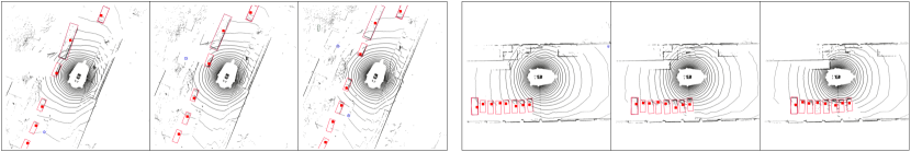
Figure 11: Detections of adjacent frames. We visualize predicted boxes and the corresponding query voxels, which are enlarged as red squares. This figure is best viewed by zoom-in.

Network Structures

We develop our VoxelNeXt network upon the widely-used residual sparse convolutional block [57, 41, 12]. We use 2D sparse convolutions in its variant of VoxelNeXt-2D. For voxel selection and box regression, we use fully-connected layer or kernel-size-3 submanifold sparse convolutions [19] for prediction. The former convolution has 128 channels in VoxelNeXt-2D and 64 in 3D networks. Training schedules and hyper-parameters follow prior works [41, 57].

The backbone network of VoxelNeXt has 6 stages. The channels for these stages are {16, 32, 64, 128, 128, 128} by default. There are 2 residual submanifold sparse convolutional blocks [19] in each stage. The sparse head predicts outputs by $3\times 3$ submainfold sparse convolutions. Following CenterPoint [57], the prediction layers are only shared among similar classes on nuScenes and Argoverse2 and shared among all classes on Waymo. The kernel sizes for the sparse max pooling layer varies in different heads, because the size of objects varies in different classes.

Appendix B Experimental results

Performance on nuScenes Validation  We provide the performance of VoxelNeXt on nuScenes val in Tab. A - 17.

Gaps between VoxelNeXt and VoxelNeXt-2D  We analyze the gaps between VoxelNeXt and VoxelNeXt-2D on different amounts of training data in Tab. A - 19. These models are trained on 1/4, 1/2, and full nuScenes training set, respectively, and evaluated on the full validation set. It shows that The gap is large on the 1/4 training data, while the gaps gradually narrow as the data amount grows. Overall, the 3D network can obtain much better performance than its 2D counterpart at a small amount of data. Meanwhile, VoxelNeXt-2D has potential on large data amount.

Resolution of Sparse Head We make an ablation study on the resolution of prediction head in Tab. A - 18. The performance decreases as the head resolution increases from the default setting of 8 to 32. In addition, we also evaluate the multi-head design of {8, 16, 32} and {2, 4, 8, 16, 32}, where results are combined from the multiple heads with various resolutions. These multi-head models present no better results than the single-resolution 8 network.

Table 20: Results on Vehicle detection on Waymo. ^∗ means decreasing the number of pasted instances in the ground-truth sampling augmentation and increase training epochs by 6 epochs [16].

Method	L1 AP/APH	L2 AP/APH
VoxelNeXt	78.2 / 77.7	69.9 / 69.4
VoxelNeXt∗	79.1 / 79.0	70.8 / 70.5

Performance on Waymo vehicle detection  In Tab. A - 20, we follow FSD [16] to decrease the number of pasted instances in the ground-truth sampling augmentation and increase training epochs by 6 epochs. This trick leads to better results upon VoxelNeXt on the Waymo object detection.

Appendix C Visualizations

We visualize the results of adjacent frames in Fig. A - 11. The corresponding query voxels are depicted as red squares.

Appendix D Discussions

Point-based Detectors  Point-based 3D object detectors [37, 43, 55, 59] are fully sparse by their very nature. Point R-CNN [43] is a pioneer work and presents decent performance on KITTI [18]. Methods of SSD series [55], including 3DSSD [55, 59], inherit the point-based tradition and accelerate the methods with simplified pipelines. VoteNet [37] is based on center voting and studies indoor 3D object detection. However, point-based detectors are usually used in scenes with limited points. The neighborhood query operation is still unaffordable in large-scale benchmarks [3, 45], which are dominated by voxel-based detectors [41, 57].

Boarder Impacts  VoxelNeXt replies on 3D data and its spatially sparse distribution. It might reflect biases in data collection, including the ones of negative societal impacts.

References

- [1] Xuyang Bai, Zeyu Hu, Xinge Zhu, Qingqiu Huang, Yilun Chen, Hongbo Fu, and Chiew-Lan Tai. Transfusion: Robust lidar-camera fusion for 3d object detection with transformers. In CVPR, pages 1080–1089, 2022.
- [2] Nuri Benbarka, Jona Schröder, and Andreas Zell. Score refinement for confidence-based 3d multi-object tracking. In IROS, pages 8083–8090, 2021.
- [3] Holger Caesar, Varun Bankiti, Alex H. Lang, Sourabh Vora, Venice Erin Liong, Qiang Xu, Anush Krishnan, Yu Pan, Giancarlo Baldan, and Oscar Beijbom. nuscenes: A multimodal dataset for autonomous driving. In CVPR, pages 11618–11628, 2020.
- [4] Qi Chen, Lin Sun, Ernest Cheung, and Alan L. Yuille. Every view counts: Cross-view consistency in 3d object detection with hybrid-cylindrical-spherical voxelization. In NeurIPS, 2020.
- [5] Qi Chen, Lin Sun, Zhixin Wang, Kui Jia, and Alan L. Yuille. Object as hotspots: An anchor-free 3d object detection approach via firing of hotspots. In ECCV, volume 12366, pages 68–84, 2020.
- [6] Yukang Chen, Yanwei Li, Xiangyu Zhang, Jian Sun, and Jiaya Jia. Focal sparse convolutional networks for 3d object detection. In CVPR, pages 5418–5427, 2022.
- [7] Yukang Chen, Yanwei Li, Xiangyu Zhang, Jian Sun, and Jiaya Jia. Focal sparse convolutional networks for 3d object detection. In CVPR, pages 5418–5427, 2022.
- [8] Yukang Chen, Jianhui Liu, Xiaojuan Qi, Xiangyu Zhang, Jian Sun, and Jiaya Jia. Scaling up kernels in 3d cnns. CoRR, abs/2206.10555, 2022.
- [9] Hsu-Kuang Chiu, Jie Li, Rares Ambrus, and Jeannette Bohg. Probabilistic 3d multi-modal, multi-object tracking for autonomous driving. In ICRA, pages 14227–14233, 2021.
- [10] Ruihang Chu, Yukang Chen, Tao Kong, Lu Qi, and Lei Li. Icm-3d: Instantiated category modeling for 3d instance segmentation. IEEE Robotics and Automation Letters, 7(1):57–64, 2021.
- [11] Ruihang Chu, Xiaoqing Ye, Zhengzhe Liu, Xiao Tan, Xiaojuan Qi, Chi-Wing Fu, and Jiaya Jia. Twist: Two-way inter-label self-training for semi-supervised 3d instance segmentation. In Proceedings of the IEEE/CVF conference on computer vision and pattern recognition, pages 1100–1109, 2022.
- [12] Jiajun Deng, Shaoshuai Shi, Peiwei Li, Wengang Zhou, Yanyong Zhang, and Houqiang Li. Voxel R-CNN: towards high performance voxel-based 3d object detection. In AAAI, pages 1201–1209, 2021.
- [13] Shengheng Deng, Zhihao Liang, Lin Sun, and Kui Jia. VISTA: boosting 3d object detection via dual cross-view spatial attention. In CVPR, pages 8438–8447, 2022.
- [14] Kaiwen Duan, Song Bai, Lingxi Xie, Honggang Qi, Qingming Huang, and Qi Tian. Centernet: Keypoint triplets for object detection. In ICCV, pages 6568–6577, 2019.
- [15] Lue Fan, Ziqi Pang, Tianyuan Zhang, Yu-Xiong Wang, Hang Zhao, Feng Wang, Naiyan Wang, and Zhaoxiang Zhang. Embracing single stride 3d object detector with sparse transformer. In CVPR, pages 8448–8458, 2022.
- [16] Lue Fan, Feng Wang, Naiyan Wang, and Zhaoxiang Zhang. Fully sparse 3d object detection. CoRR, abs/2207.10035, 2022.
- [17] Lue Fan, Xuan Xiong, Feng Wang, Naiyan Wang, and Zhaoxiang Zhang. Rangedet: In defense of range view for lidar-based 3d object detection. In ICCV, pages 2898–2907, 2021.
- [18] Andreas Geiger, Philip Lenz, Christoph Stiller, and Raquel Urtasun. Vision meets robotics: The KITTI dataset. Int. J. Robotics Res., 32(11):1231–1237, 2013.
- [19] Benjamin Graham, Martin Engelcke, and Laurens van der Maaten. 3d semantic segmentation with submanifold sparse convolutional networks. In CVPR, pages 9224–9232, 2018.
- [20] Tianrui Guan, Jun Wang, Shiyi Lan, Rohan Chandra, Zuxuan Wu, Larry Davis, and Dinesh Manocha. M3DETR: multi-representation, multi-scale, mutual-relation 3d object detection with transformers. In WACV, pages 2293–2303, 2022.
- [21] Chenhang He, Ruihuang Li, Shuai Li, and Lei Zhang. Voxel set transformer: A set-to-set approach to 3d object detection from point clouds. In CVPR, pages 8407–8417, 2022.
- [22] Yihan Hu, Zhuangzhuang Ding, Runzhou Ge, Wenxin Shao, Li Huang, Kun Li, and Qiang Liu. Afdetv2: Rethinking the necessity of the second stage for object detection from point clouds. In AAAI, pages 969–979, 2022.
- [23] Li Jiang, Shaoshuai Shi, Zhuotao Tian, Xin Lai, Shu Liu, Chi-Wing Fu, and Jiaya Jia. Guided point contrastive learning for semi-supervised point cloud semantic segmentation. In CVPR, pages 6423–6432, 2021.
- [24] Diederik P. Kingma and Jimmy Ba. Adam: A method for stochastic optimization. In Yoshua Bengio and Yann LeCun, editors, ICLR, 2015.
- [25] Xin Lai, Yukang Chen, Fanbin Lu, Jianhui Liu, and Jiaya Jia. Spherical transformer for lidar-based 3d recognition. In CVPR, 2023.
- [26] Xin Lai, Jianhui Liu, Li Jiang, Liwei Wang, Hengshuang Zhao, Shu Liu, Xiaojuan Qi, and Jiaya Jia. Stratified transformer for 3d point cloud segmentation. In Proceedings of the IEEE/CVF Conference on Computer Vision and Pattern Recognition, pages 8500–8509, 2022.
- [27] Alex H. Lang, Sourabh Vora, Holger Caesar, Lubing Zhou, Jiong Yang, and Oscar Beijbom. Pointpillars: Fast encoders for object detection from point clouds. In CVPR, pages 12697–12705, 2019.
- [28] Yanwei Li, Yilun Chen, Xiaojuan Qi, Zeming Li, Jian Sun, and Jiaya Jia. Unifying voxel-based representation with transformer for 3d object detection. CoRR, abs/2206.00630, 2022.
- [29] Zhichao Li, Feng Wang, and Naiyan Wang. Lidar R-CNN: an efficient and universal 3d object detector. In CVPR, pages 7546–7555, 2021.
- [30] Tingting Liang, Hongwei Xie, Kaicheng Yu, Zhongyu Xia, Zhiwei Lin, Yongtao Wang, Tao Tang, Bing Wang, and Zhi Tang. Bevfusion: A simple and robust lidar-camera fusion framework. CoRR, abs/2205.13790, 2022.
- [31] Tsung-Yi Lin, Priya Goyal, Ross B. Girshick, Kaiming He, and Piotr Dollár. Focal loss for dense object detection. T-PAMI, 42(2):318–327, 2020.
- [32] Jianhui Liu, Yukang Chen, Xiaoqing Ye, Zhuotao Tian, Xiao Tan, and Xiaojuan Qi. Spatial pruned sparse convolution for efficient 3d object detection. In NeurIPS, 2022.
- [33] Zhijian Liu, Haotian Tang, Alexander Amini, Xinyu Yang, Huizi Mao, Daniela Rus, and Song Han. Bevfusion: Multi-task multi-sensor fusion with unified bird’s-eye view representation. CoRR, abs/2205.13542, 2022.
- [34] Jiageng Mao, Minzhe Niu, Haoyue Bai, Xiaodan Liang, Hang Xu, and Chunjing Xu. Pyramid R-CNN: towards better performance and adaptability for 3d object detection. In ICCV, 2021.
- [35] Jiageng Mao, Yujing Xue, Minzhe Niu, Haoyue Bai, Jiashi Feng, Xiaodan Liang, Hang Xu, and Chunjing Xu. Voxel transformer for 3d object detection. In ICCV, 2021.
- [36] Ziqi Pang, Zhichao Li, and Naiyan Wang. Simpletrack: Understanding and rethinking 3d multi-object tracking. CoRR, abs/2111.09621, 2021.
- [37] Charles R. Qi, Or Litany, Kaiming He, and Leonidas J. Guibas. Deep hough voting for 3d object detection in point clouds. In ICCV, pages 9276–9285, 2019.
- [38] Charles Ruizhongtai Qi, Li Yi, Hao Su, and Leonidas J. Guibas. Pointnet++: Deep hierarchical feature learning on point sets in a metric space. In NeurIPS, pages 5099–5108, 2017.
- [39] Shaoqing Ren, Kaiming He, Ross B. Girshick, and Jian Sun. Faster R-CNN: towards real-time object detection with region proposal networks. In NeurIPS, pages 91–99, 2015.
- [40] Guangsheng Shi, Ruifeng Li, and Chao Ma. Pillarnet: Real-time and high-performance pillar-based 3d object detection. CoRR, abs/2205.07403, 2022.
- [41] Shaoshuai Shi, Chaoxu Guo, Li Jiang, Zhe Wang, Jianping Shi, Xiaogang Wang, and Hongsheng Li. PV-RCNN: point-voxel feature set abstraction for 3d object detection. In CVPR, pages 10526–10535, 2020.
- [42] Shaoshuai Shi, Li Jiang, Jiajun Deng, Zhe Wang, Chaoxu Guo, Jianping Shi, Xiaogang Wang, and Hongsheng Li. PV-RCNN++: point-voxel feature set abstraction with local vector representation for 3d object detection. CoRR, abs/2102.00463, 2021.
- [43] Shaoshuai Shi, Xiaogang Wang, and Hongsheng Li. Pointrcnn: 3d object proposal generation and detection from point cloud. In CVPR, pages 770–779, 2019.
- [44] Shaoshuai Shi, Zhe Wang, Jianping Shi, Xiaogang Wang, and Hongsheng Li. From points to parts: 3d object detection from point cloud with part-aware and part-aggregation network. T-PAMI, 43(8):2647–2664, 2021.
- [45] Pei Sun and et. al. Scalability in perception for autonomous driving: Waymo open dataset. In CVPR, pages 2443–2451, 2020.
- [46] Pei Sun, Mingxing Tan, Weiyue Wang, Chenxi Liu, Fei Xia, Zhaoqi Leng, and Dragomir Anguelov. Swformer: Sparse window transformer for 3d object detection in point clouds. CoRR, abs/2210.07372, 2022.
- [47] Pei Sun, Weiyue Wang, Yuning Chai, Gamaleldin Elsayed, Alex Bewley, Xiao Zhang, Cristian Sminchisescu, and Dragomir Anguelov. RSN: range sparse net for efficient, accurate lidar 3d object detection. In CVPR, pages 5725–5734, 2021.
- [48] Dominic Zeng Wang and Ingmar Posner. Voting for voting in online point cloud object detection. In Robotics: Science and Systems, 2015.
- [49] Jun Wang, Shiyi Lan, Mingfei Gao, and Larry S. Davis. Infofocus: 3d object detection for autonomous driving with dynamic information modeling. In ECCV, volume 12355, pages 405–420, 2020.
- [50] Yue Wang, Alireza Fathi, Abhijit Kundu, David A. Ross, Caroline Pantofaru, Thomas A. Funkhouser, and Justin M. Solomon. Pillar-based object detection for autonomous driving. In ECCV, 2020.
- [51] Xinshuo Weng, Jianren Wang, David Held, and Kris Kitani. 3d multi-object tracking: A baseline and new evaluation metrics. In IROS, pages 10359–10366, 2020.
- [52] Benjamin Wilson and et. al. Argoverse 2: Next generation datasets for self-driving perception and forecasting. In NeurIPS, 2021.
- [53] Yan Yan, Yuxing Mao, and Bo Li. SECOND: sparsely embedded convolutional detection. Sensors, 18(10):3337, 2018.
- [54] Honghui Yang, Zili Liu, Xiaopei Wu, Wenxiao Wang, Wei Qian, Xiaofei He, and Deng Cai. Graph r-cnn: Towards accurate 3d object detection with semantic-decorated local graph. In ECCV, 2022.
- [55] Zetong Yang, Yanan Sun, Shu Liu, and Jiaya Jia. 3dssd: Point-based 3d single stage object detector. In CVPR, pages 11037–11045, 2020.
- [56] Zetong Yang, Yin Zhou, Zhifeng Chen, and Jiquan Ngiam. 3d-man: 3d multi-frame attention network for object detection. In CVPR, pages 1863–1872, 2021.
- [57] Tianwei Yin, Xingyi Zhou, and Philipp Krähenbühl. Center-based 3d object detection and tracking. In CVPR, pages 11784–11793, 2021.
- [58] Jan-Nico Zaech, Dengxin Dai, Alexander Liniger, Martin Danelljan, and Luc Van Gool. Learnable online graph representations for 3d multi-object tracking. CoRR, abs/2104.11747, 2021.
- [59] Yifan Zhang, Qingyong Hu, Guoquan Xu, Yanxin Ma, Jianwei Wan, and Yulan Guo. Not all points are equal: Learning highly efficient point-based detectors for 3d lidar point clouds. In CVPR, pages 18931–18940, 2022.
- [60] Xingyi Zhou, Vladlen Koltun, and Philipp Krähenbühl. Tracking objects as points. In ECCV, volume 12349, pages 474–490, 2020.
- [61] Yin Zhou and Oncel Tuzel. Voxelnet: End-to-end learning for point cloud based 3d object detection. In CVPR, pages 4490–4499, 2018.
- [62] Benjin Zhu, Zhengkai Jiang, Xiangxin Zhou, Zeming Li, and Gang Yu. Class-balanced grouping and sampling for point cloud 3d object detection. CoRR, abs/1908.09492, 2019.