Exclusive semileptonic $B_{s}\to K\ell\nu$ decays on the lattice

Abstract

Semileptonic $B_{s}\to K\ell\nu$ decays provide an alternative $b$-decay channel to determine the CKM matrix element $|V_{ub}|$, and to obtain a $R$-ratio to investigate lepton-flavor-universality violations. Results for the CKM matrix element may also shed light on the discrepancies seen between analyses of inclusive or exclusive decays. We calculate the decay form factors using lattice QCD with domain-wall light quarks and a relativistic $b$-quark. We analyze data at three lattice spacings with unitary pion masses down to $268\,\text{MeV}$. Our numerical results are interpolated/extrapolated to physical quark masses and to the continuum to obtain the vector and scalar form factors $f_{+}(q^{2})$ and $f_{0}(q^{2})$ with full error budgets at $q^{2}$ values spanning the range accessible in our simulations. We provide a possible explanation of tensions found between results for the form factor from different lattice collaborations. Model- and truncation-independent $z$-parameterization fits following a recently proposed Bayesian-inference approach extend our results to the entire allowed kinematic range. Our results can be combined with experimental measurements of $B_{s}\to D_{s}$ and $B_{s}\to K$ semileptonic decays to determine $|V_{ub}|=3.8(6)\times 10^{-3}$. The error is currently dominated by experiment. We compute differential branching fractions and two types of $R$ ratios, the one commonly used as well as a variant better suited to test lepton-flavor universality.

I Introduction

High-precision tests of the Standard Model (SM) from flavor physics are an important complement to direct searches at colliders for new physics. The absence of tree-level flavor-changing neutral currents in the SM provides one window where new physics effects could be seen, though it is important to test high-precision calculations of both tree- and loop-level SM processes against experiment.

New physics is expected to occur at higher energy scales and seeing its effects is more likely if the decaying particle can release large amounts of energy. Decays of mesons containing a heavy $b$-quark provide many opportunities because the $b$-quark lives long enough for experimental investigation but also delivers more than $4\,\text{GeV}$ of energy. The large $b$-quark mass allows a plethora of decay channels and correspondingly many tests of the SM. Tantalizing deviations between SM predictions and experimental measurements have been reported [1, 2, 3, 4, 5, 6]. While the latest experimental LHCb results [7] confirm the universality of lepton families under the weak interaction, the high-energy reach of flavor physics continues to make it a primary probe for the search of beyond-SM physics.

Here we focus on $B_{s}$-meson decay arising at tree level in the SM with a kaon in the final state. Lattice results over the full $q^{2}$ range for $B_{s}\to K\ell\nu$ form factors have been obtained by HPQCD [8, 9], RBC-UKQCD [10], and Fermilab-MILC [11], as well as at a single $q^{2}$ value by the Alpha collaboration [12]. Recent lattice results for $B_{s}\to K\ell\nu$ semileptonic decays are summarized in Refs. [13, 14] and [15].

$B_{s}\to K\ell\nu$ decays have been observed by LHCb [16] and can be used to obtain the magnitudes of the CKM matrix elements $|V_{ub}|$. Using these alternative $b$-decay channels may shed light on the use of different kinematical parameterizations for the exclusive decay form factors and on tensions within and between extractions of $|V_{ub}|$ from inclusive or exclusive decays.

The remainder of this paper is structured as follows. In Section II we describe the form factors we will compute and provide the details of our lattice computation. In Section III we describe the statistical analysis of the lattice data. In Section IV we determine estimates for all sources of uncertainties and thereby assemble a complete error budget. Section V discusses the extrapolation of the obtained form factors over the full kinematical range and provides a wealth of quantities of phenomenological interest before we conclude in Section VI.

II Lattice calculation

II.1 Form factors

We work in the $B_{s}$-meson rest frame for our calculations. For $\bar{B}^{0}_{s}\to K^{+}\ell^{-}\bar{\nu}_{\ell}$, the differential decay rate in this frame is given by

$$\frac{d\Gamma(B_{s}{\to}K\ell\nu)}{dq^{2}}= \eta_{\text{EW}}\frac{G_{F}^{2}|V_{ub}|^{2}}{24\pi^{3}}\,\frac{(q^{2}{-}m_{\ell}^{2})^{2}|{\bf p}_{K}|}{(q^{2})^{2}}$$

$$\times\bigg{[}\Big{(}1{+}\frac{m_{\ell}^{2}}{2q^{2}}\Big{)}|{\bf p}_{K}|^{2}|f_{+}(q^{2})|^{2}$$

$$+\frac{3m_{\ell}^{2}}{8q^{2}}\frac{(M_{B_{s}}^{2}{-}M_{K}^{2})^{2}}{M_{B_{s}}^{2}}|f_{0}(q^{2})|^{2}\bigg{]}\,.$$ (1)

The $4$-momenta of the $B_{s}$ and the final-state kaon are denoted by $p_{B_{s}}$ and $p_{K}$ respectively. $M_{B_{s}}$ and $M_{K}$ denote the corresponding meson masses, $E_{K}$ is the $K$-meson energy, $|{\bf p}_{K}|=(E_{K}^{2}-M_{K}^{2})^{1/2}$, and $q=p_{B_{s}}-p_{K}$ is the momentum transfer between the $B_{s}$ and $K$ mesons. $\eta_{\text{EW}}$ is an electroweak correction factor. The form factors $f_{+}$ and $f_{0}$ arise in the decomposition of the QCD matrix element

$$\langle K(p_{K})|\mathcal{V}^{\mu}|B_{s}(p_{B_{s}})\rangle=\\ f_{+}(q^{2})\bigg{(}p_{K}^{\mu}+p_{B_{s}}^{\mu}-q^{\mu}\frac{M_{B_{s}}^{2}-M_{K}^{2}}{q^{2}}\bigg{)}\\ +f_{0}(q^{2})\frac{M_{B_{s}}^{2}-M^{2}_{K}}{q^{2}}q^{\mu}.$$ (2)

In the SM, $\mathcal{V}^{\mu}=\bar{u}\gamma^{\mu}b$ is the continuum charged current operator. For lattice simulations it is convenient to use the alternative parameterization

$$\langle K|\mathcal{V}^{\mu}|B_{s}\rangle=\sqrt{2M_{B_{s}}}\,\big{[}v^{\mu}f_{\parallel}(E_{K})+p^{\mu}_{\perp}f_{\perp}(E_{K})\big{]}\,,$$ (3)

and the relations

$$f_{0}(q^{2}) =\frac{\sqrt{2M_{B_{s}}}}{M^{2}_{B_{s}}{-}M^{2}_{K}}\big{[}(M_{B_{s}}{-}E_{K})f_{\parallel}(E_{K})$$

$$\hskip 51.6665pt+(E_{K}^{2}{-}M^{2}_{K})f_{\perp}(E_{K})\big{]},$$ (4)

$$f_{+}(q^{2}) =\frac{1}{\sqrt{2M_{B_{s}}}}\left[f_{\parallel}(E_{K})+(M_{B_{s}}-E_{K})f_{\perp}(E_{K})\right]\,,$$ (5)

where $v$ is the $B_{s}$ meson $4$-velocity, ${(p_{B_{s}})}^{\mu}_{\perp}\equiv p_{K}^{\mu}-(p_{K}\cdot v)v^{\mu}$ and, in the $B_{s}$ meson rest frame,

$$f_{\parallel}(E_{K})=\frac{\langle K|\mathcal{V}^{0}|B_{s}\rangle}{\sqrt{2M_{B_{s}}}},\quad f_{\perp}(E_{K})=\frac{1}{p_{K}^{i}}\,\frac{\langle K|\mathcal{V}^{i}|B_{s}\rangle}{\sqrt{2M_{B_{s}}}}.$$ (6)

We note that no Einstein summation convention is applied in the second equation; it holds component-by-component for the non-zero components of ${p}_{K}^{i}$.

II.2 Action and parameters

Table 1: RBC/UKQCD coarse (C), medium (M) and fine (F) gauge field ensembles [19, 20, 21, 22] used in this calculation, with $2+1$-flavor domain-wall fermions and Iwasaki-gauge action. The domain-wall height for light and strange quarks is $M_{5}=1.8$. The ensembles are generated using the Shamir domain-wall kernel [23, 24]. $am_{l}$ denotes the light sea-quark mass and $am_{s}^{\text{sea}}$ the strange sea-quark mass. The lattice spacing and physical strange quark were obtained in the combined analysis of Refs. [21, 22, 25]. The valence strange-quark masses used in our simulations on the C(M) ensembles are $am_{s}^{\text{sim}}=0.03224\,(0.025)$, while on F1S we used $am_{s}^{\text{sim}}=am_{s}^{\text{sea}}$.

$$\begin{array}[]{cccccccccccc}\hline\cr\hline\cr&L/a&T/a&L_{s}&a^{-1}\!/\!\,\text{GeV}&am_{l}&am_{s}^{\text{sea}}&am_{s}^{\text{phys}}&M_{\pi}/\!\,\text{MeV}&\text{\# cfgs}&\text{\# sources}\\ \hline\cr\text{C1}&24&64&16&1.7848(50)&0.005&0.040&0.03224(18)&340&1636&1\\ \text{C2}&24&64&16&1.7848(50)&0.010&0.040&0.03224(18)&434&1419&1\\[5.16663pt] \text{M1}&32&64&16&2.3833(86)&0.004&0.030&0.02477(18)&301&628&2\\ \text{M2}&32&64&16&2.3833(86)&0.006&0.030&0.02477(18)&363&889&2\\ \text{M3}&32&64&16&2.3833(86)&0.008&0.030&0.02477(18)&411&544&2\\[5.16663pt] \text{F1S}&48&96&12&2.785(11)&0.002144&0.02144&0.02167(20)&268&98&24\\ \hline\cr\hline\cr\end{array}$$

Our calculations are based on a subset of RBC-UKQCD’s $2+1$ flavor domain-wall fermion and Iwasaki gauge-field ensembles [19, 20, 21, 22] which we summarize in Table 1. Our dataset includes six ensembles at three different lattice spacings, with pion masses down to $268\,\text{MeV}$. Light and strange quarks are simulated using domain-wall fermions [26, 23, 24, 27, 28, 29]. The light (up and down) sea-quark masses are degenerate and correspond to pion masses in the range $268\,\text{MeV}\leq M_{\pi}\leq 434\,\text{MeV}$. The strange sea-quark mass is within $20$ to $25\%$ of its physical value on the C and M ensembles, and is tuned to a deviation of $1\%$ on the F1S ensemble.

Bottom quarks are simulated using the relativistic heavy quark (RHQ) action [30, 31], a variant of the Fermilab action [32] with three non-perturbatively tuned parameters [33]. The RHQ tuning determines the bare-quark mass, $m_{0}a$, clover coefficient, $c_{P}$, and anisotropy parameter, $\zeta$, in the RHQ action using as inputs the experimentally measured $B_{s}$-meson mass and hyperfine splitting, together with the constraint that the lattice rest mass (measured from the exponential decay of meson correlation functions) equals the kinetic mass (measured from the meson dispersion relation). The outputs of the RHQ tuning for the ensembles used here are given in Table 17, with details of the procedure in appendix A.

Light and strange quarks are generated using point sources, whereas $b$ quarks are generated using a Gaussian smeared source [34, 35] in order to reduce excited-state contamination. We use the smearing parameters that were determined in Ref. [33] and list them in Tab. 13 in appendix A.

Our data is generated using the lattice QCD software packages Qlua [36] and Chroma [37]. Further details of the set-up can be found in Refs. [38, 10, 39, 22, 25].

II.3 Operator renormalization and improvement

Matrix elements from our simulations are matched to continuum ones using the relation

$$\langle K|\mathcal{V}_{\mu}|B_{s}\rangle=Z^{bl}_{V_{\mu}}\langle K|V_{\mu}|B_{s}\rangle\,,$$ (7)

where $l$ stands for the light quark and we denote the continuum and lattice currents by $\mathcal{V}_{\mu}$ and $V_{\mu}$, respectively. The renormalization factor

$$Z^{bl}_{V_{\mu}}=\rho^{bl}_{V_{\mu}}\sqrt{Z^{ll}_{V}Z^{bb}_{V}}\,,$$ (8)

is obtained following Refs. [40, 41]. The flavor-conserving renormalization factors $Z^{ll}_{V}$ and $Z^{bb}_{V}$ account for most of the operator renormalization, while $\rho^{bl}_{V_{\mu}}$ is a residual correction, expected to be close to unity because most of the radiative corrections, including tadpoles, cancel [42]. We obtain $Z^{bb}_{V}$ non-perturbatively from the matrix element of the $b\to b$ vector current between two $B_{s}$ mesons:

$$Z_{V}^{bb}\langle B_{s}|V_{0}|B_{s}\rangle=2M_{B_{s}}.$$ (9)

Details of the calculation are given in appendix A of Ref. [38]. The light-light renormalization factor was calculated from $Z_{A}^{ll}$ [20] using the relation $Z_{V}^{ll}=Z_{A}^{ll}$ to $O(am_{\text{res}})$ for domain-wall fermions.

Following our previous work [10], we improve the heavy-light vector current to $O(\alpha_{s}a)$ using the following operators

$$V_{0}^{\rm imp}(x) =V_{0}^{0}(x)+c_{t}^{3}V_{0}^{3}(x)+c_{t}^{4}V_{0}^{4}(x),$$ (10)

$$V_{i}^{\rm imp}(x) =V_{i}^{0}(x)$$ (11)

$$\phantom{={}}+c_{s}^{1}V_{i}^{1}(x)+c_{s}^{2}V_{i}^{2}(x)+c_{s}^{3}V_{i}^{3}(x)+c_{s}^{4}V_{i}^{4}(x)\,.$$

where $c_{t}^{n}$ and $c_{s}^{n}$ are coefficients and

$$V_{\mu}^{0}(x) =\bar{\psi}(x)\gamma^{\mu}Q(x),$$ (12)

$$V_{\mu}^{1}(x) =\bar{\psi}(x)2\overrightarrow{D}_{\mu}Q(x),$$ (13)

$$V_{\mu}^{2}(x) =\bar{\psi}(x)2\overleftarrow{D}_{\mu}Q(x),$$ (14)

$$V_{\mu}^{3}(x) =\bar{\psi}(x)2\gamma_{\mu}\gamma_{i}\overrightarrow{D}_{i}Q(x),$$ (15)

$$V_{\mu}^{4}(x) =\bar{\psi}(x)2\gamma_{\mu}\gamma_{i}\overleftarrow{D}_{i}Q(x),$$ (16)

with $\psi$ a light quark and $Q$ an RHQ quark. The covariant derivatives are given by

$$\overrightarrow{D}_{\mu}Q(x) =\frac{1}{2}\big{(}U_{\mu}(x)Q(x+\hat{\mu})-U_{\mu}^{\dagger}(x-\hat{\mu})Q(x-\hat{\mu})\big{)},$$ (17)

$$\bar{\psi}(x)\overleftarrow{D}_{\mu} =\frac{1}{2}\big{(}\bar{\psi}(x+\hat{\mu})U_{\mu}^{\dagger}(x)-\bar{\psi}(x-\hat{\mu})U_{\mu}(x-\hat{\mu})\big{)}.$$ (18)

Both the residual renormalization factor $\rho^{bl}_{V}$ and the coefficients $c_{t}^{n}$ and $c_{s}^{n}$ were computed at one-loop order [43] in mean-field improved lattice perturbation theory [44], with the results given in Table 20 in Appendix C.

II.4 Setup of the calculation

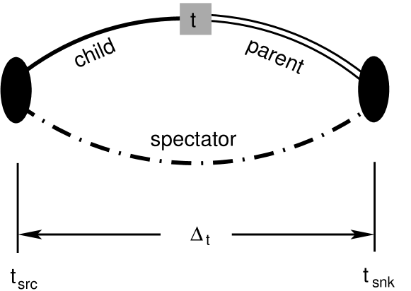
Figure 1: Sketch of the construction of the three-point function in the “forward direction”. The strange spectator quark (dash-dotted line) originates from time slice $t_{\mathrm{src}}$ and propagates forward to time slice $t_{\text{snk}}$ where we create a point sink and turn it into a sequential source for the parent $b$ quark (double line) propagating backwards. This sequential propagator is contracted with the child light quark (solid line) also originating from $t_{\mathrm{src}}$. The contraction of child and parent quark (gray box) is calculated inserting the operators for the vector current and varied over the time slices $t_{\mathrm{src}}$ to $t_{\text{snk}}$.

In Fig. 1 we sketch our calculation of three-point correlation functions using sequential propagators separating initial and final state by $\Delta_{t}$ [45]. The initial $B_{s}$ meson is located at $t_{\text{snk}}=t_{\mathrm{src}}+\Delta_{t}$, whereas the final state kaon is at $t_{\mathrm{src}}$. We proceed by letting the strange spectator quark propagate from $t=t_{\mathrm{src}}$ to $t=t_{\text{snk}}$ where we give it a sink which is turned into the sequential source for the parent $b$ quark. The $b$ quark is contracted with a child light quark also starting at $t=t_{\mathrm{src}}$ over all time slices in the range $t_{\mathrm{src}}\leq t\leq t_{\text{snk}}$. The contraction is calculated inserting the operators for the vector current defined in Eqs. (12)-(16). In addition to the shown setup in the “forward” direction, we effectively double statistics by calculating the “backward” direction, i.e. we use a second sink location at $t^{\prime}_{\text{snk}}=t_{\mathrm{src}}-\Delta_{t}$. For each configuration, we first average forward and backward three-point correlators before proceeding with the analysis. This step is similar to “folding” two-point correlators about the central time slice in order to take advantage of the symmetry of forward- and backward-propagating states.

We use one time source at $t_{\mathrm{src}}/a=0$ for the coarse C1 and C2 ensembles, two time sources at $t_{\mathrm{src}}/a=0,\,32$ for the medium M1, M2, and M3 ensembles, and 24 time sources separated by four time slices on the F1S ensemble. The separation $\Delta_{t}$ on ensembles C1, C2, M1, M2 and M3 is the same as in our previous work [10] where we carefully studied several source-sink separations to cleanly identify the ground-state signal. On the F1S ensemble we generated data for multiple source-sink separations ($\Delta_{t}/a=30,32,34$) to study the effects of excited states. We found that the signal saturates for $\Delta_{t}/a=32$ with the centre of the signal region being ground-state dominated and compatible with the $\Delta_{t}/a=34$ dataset. We therefore chose $\Delta_{t}/a=32$ for our final analysis. We keep $\Delta_{t}$ nearly constant in physical units we choose $\Delta_{t}/a=20$, 26, and 32 for the three lattice spacings corresponding to the C, M, and F ensembles, respectively. In order to further decorrelate measurements, we perform a random 4-vector shift on the gauge field prior to placing any source. This 4-vector shift is equivalent to randomly choosing the first source position on each configuration but simplifies the bookkeeping.

The initial $B_{s}$ meson is kept at rest and momentum is inserted in the final state through the current operator. The simulations use strange spectator quarks with a mass close to the physical value (see Tab. 1) and we tune the RHQ parameters such that the parent quark corresponds to a physical $b$ quark. The child light quark is unitary and has the same mass as the light sea quarks.

III Analysis

The analysis to extract form factor results is implemented ensemble-by-ensemble as a simultaneous correlated frequentist fit over two-point and three-point correlation functions to obtain masses and the lattice form factors $f_{\|}$ and $f_{\perp}$ for all simulated momentum transfers, i.e. one single fit per ensemble. These form factors are then renormalized and converted to $f_{+}$ and $f_{0}$ using Eqs. (II.1) and (5). They are subsequently interpolated/extrapolated to physical quark masses and to the continuum limit in a single step. We use bootstrap resampling [46] with 1000 samples.

III.1 Two-point correlation function fits

Here we describe individual correlated fits to the $\pi$, $K$ and $B_{s}$ two-point data. The results for the pion mass determined here will enter subsequent analyses. For $K$ and $B_{s}$ this section only serves to determine optimal fit-ranges, which we use in the next section for the combined fit with ratios of three-point and two-point correlators.

The functional form of the two-point correlation functions $C_{2}$ is given by

$$C^{P}_{2}(t,T,{\bf p}_{P}) =\sum_{{\bf x}}e^{i{\bf p}_{P}\cdot{\bf x}}\langle\mathcal{O}_{\mathrm{snk}}({\bf x},t)\mathcal{O}^{\dagger}_{\mathrm{src}}({\bf 0},0)\rangle$$

$$=\sum_{n=0}^{N}\langle 0|\mathcal{O}_{\mathrm{snk}}|X^{(n)}\rangle\langle X^{(n)}|\mathcal{O}^{\dagger}_{\mathrm{src}}|0\rangle$$

$$\quad\times\left(\frac{e^{-E_{P,n}t}+e^{-E_{P,n}(T-t)}}{2E_{P,n}}\right),$$ (19)

where the interpolating operators $\mathcal{O}_{\mathrm{src}}$, $\mathcal{O}_{\mathrm{snk}}$ are given by $\bar{l}\gamma^{5}l$, $\bar{s}\gamma^{5}l$ and $\bar{b}\gamma^{5}s$, and are chosen to induce states with the quantum numbers of the $\pi$, $K$ and $B_{s}$, respectively.

In a first step, we extract the energies $E_{P,n}$ and amplitudes $\left<X^{(n)}\vphantom{\mathcal{O}0}\right|\mathcal{O}\left|0\vphantom{X^{(n)}\mathcal{O}}\right>$ for $n=0,1$ separately for the $\pi$, $K$ and $B_{s}$ meson by fitting the correlation functions to the functional form given in Eq. (19) with $N=1$. For the $B_{s}$ mesons we simultaneously fit the smeared-sink and point-sink correlation functions under the constraint that they both describe the same meson energy. The fit ranges are determined in such a way that the inclusion of the ground and excited state visibly describes the data well, while also providing an acceptable $p$-value. Furthermore, we check that the results are stable under variations of the fit range.

The energies of the final-state kaon can be related to its rest mass via the continuum ($E_{K}^{2}=M_{K}^{2}+{\bf p}_{K}^{2}$) or the lattice dispersion relation,

$$\sinh^{2}\Big{(}\frac{aE_{K}(aM_{K},a{\bf p}_{K})}{2}\Big{)}=\\ \sinh^{2}\Big{(}\frac{aM_{K}}{2}\Big{)}+\sum_{i=1}^{3}\sin^{2}\Big{(}\frac{ap_{K,i}}{2}\Big{)}\,.$$ (20)

We have tested that the data is described by the dispersion relation using lattice momenta ${\bf p}_{K}=2\pi{\bf n}/L$ with ${\bf n}^{2}=0,1,2,3,4$, where equivalent three-momenta are averaged. This justifies imposing the lattice dispersion relation in the combined fit that we will describe in the next section. We will also compare these results with those based on the continuum dispersion relation in order to assess systematic effects.

III.2 Form factors from global fits

Without loss of generality we assume $t_{\mathrm{src}}=0$ in the following. The three-point correlation functions for the transition $B_{s}\to K$ have the functional form

$$C_{3,\mu} (t,\Delta_{t},{\bf p}_{K})$$

$$= \sum_{\bf x,y}e^{i{\bf p}_{K}\cdot{\bf y}}\langle\mathcal{O}_{\mathrm{B_{s}}}({\bf x},\Delta_{t})V_{\mu}^{\text{imp}}({\bf y},t)\mathcal{O}^{\dagger}_{K}({\bf 0},0)\rangle$$

$$= \sum_{n,m}\langle 0|\mathcal{O}_{B_{s}}|B_{s}^{(n)}\rangle\langle B_{s}^{(n)}|V^{\mathrm{imp}}_{\mu}|K^{(m)}\rangle\langle K^{(m)}|\mathcal{O}^{\dagger}_{K}|0\rangle$$

$$\qquad\quad\times\frac{e^{-E_{K,m}t}e^{-M_{B_{s},n}(\Delta_{t}-t)}}{4E_{K,m}M_{B_{s},n}},$$ (21)

where $V^{\text{imp}}_{\mu}$ are the improved lattice temporal and spatial vector currents from Eqs. (10) and (11). We notice that our notation suppresses the fact that the operators inducing the $B_{s}$ mesons can be either smeared or local at the sink. Furthermore, we neglect around-the-world-effects due to the finite temporal extent $T$ as these are suppressed by $e^{-E_{K}(T-\Delta_{t})}$.

To determine the form factors $f_{\|}$ and $f_{\perp}$ (compare Eq. (6)) we require the ground-state matrix element $\left<K\vphantom{V_{\mu}^{\mathrm{imp}}B_{s}}\right|V_{\mu}^{\mathrm{imp}}\left|B_{s}\vphantom{KV_{\mu}^{\mathrm{imp}}}\right>$ (where for convenience we dropped the superscript $(0)$). To this end we define the ratio $R_{3,\mu}(t,t_{\mathrm{snk}},{\bf p}_{K})$ as

$$R_{3,\mu}(t,t_{\text{snk}},{\bf p}_{K})=\\ \frac{C_{3,\mu}(t,t_{\text{snk}},{\bf p}_{K})}{\sqrt{C_{2}^{K}(t,{\bf p}_{K})C_{2}^{B_{s}}(t_{\text{snk}}{-}t,{\bf 0})}}\sqrt{\frac{2E_{K,0}}{e^{-E_{K,0}t-M_{B_{s},0}(t_{\text{snk}}-t)}}},$$ (22)

where we ensure that the appropriate smearing is used to cancel the overlap factors between the three-point and two-point correlation functions. By construction, these ratios satisfy

$$f_{\parallel}^{\mathrm{bare}}({\bf p}_{K}) =\lim_{0\ll t\ll t_{\mathrm{snk}}}R_{3,0}(t,t_{\mathrm{snk}},{\bf p}_{K})$$ (23)

$$f_{\perp}^{\mathrm{bare}}({\bf p}_{K}) =\lim_{0\ll t\ll t_{\mathrm{snk}}}\frac{1}{p^{i}_{K}}R_{3,i}(t,t_{\mathrm{snk}},{\bf p}_{K}),$$

so that we can obtain the form factors $f^{\mathrm{bare}}_{\parallel}$ and $f^{\mathrm{bare}}_{\perp}$ by fitting the ratio $R_{3,\mu}$.

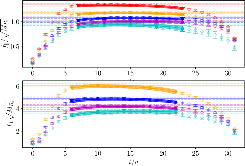
Figure 2: Example extraction of $f_{\|}$ (top) and $f_{\perp}$ (bottom) on the F1S ensemble from a correlated global fit. The different colors are for different momenta ${\bf n}2\pi/L$ injected at the current. The plot shows the fit including excited-state contributions as well as the ground-sate contribution (horizontal dashed lines). Filled symbols indicate the points that were included in the fits.

In practice, we carry out a simultaneous correlated fit over the point-point $K$ and smeared-point and point-point $B_{s}$ two-point functions (including one excited state in both cases), together with all components $\mu$ of the three-point correlation functions. For the latter we simultaneously fit over results for all momenta including ground-state-$B_{s}$-to-excited-$K$ and excited-$B_{s}$-to-ground-state-$K$ terms for the matrix element of the current. Throughout this fit we enforce the lattice dispersion relation to describe the energy levels of the kaon (c.f. Eq. (20)). Except for the results on F1S, for momenta ${\bf n}^{2}=3,4$ the statistical noise on the three-point functions is too large to allow for meaningful constraints on the latter matrix element, and we do not include it in the fit. The term containing both the $B_{s}$ and $K$ excited states leads to poorly-constrained fits and is excluded. The inclusion of excited-states allows us to extend the range of time slices we can fit, as illustrated in figure 2. In order to limit the impact of strong correlations between neighboring time slices in the ratio $R_{3,\mu}$ only every 4th time slice enters the fit. We choose fit ranges which visibly describe the data well while still giving acceptable $p$-values. The results for the ground-state matrix elements determined in this way show no dependence on the choice of lower and upper end of the fit range for the ratio when varied by $\pm 1$ time slices. An example for this fit is shown in Fig. 2

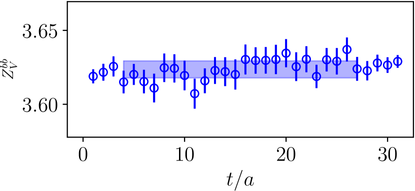
Figure 3: Example extraction of the vector-current renormalization constant $Z_{V}^{bb}$ on the F1S ensemble.

Table 2: Numerical values of the renormalization constants $Z_{A}^{ll}$ and $Z_{V}^{bb}$.

	C1	C2	M1	M2	M3	F1S
$Z_{A}^{ll}$	0.7172	0.7178	0.7449	0.7452	0.7452	0.7624
$Z_{V}^{bb}$	9.099(24)	9.135(23)	4.7767(87)	4.7602(75)	4.770(10)	3.6236(57)

What remains is to extract $Z_{V}^{bb}$. We first consider the temporal component of the zero-momentum matrix element for the $b\to b$ vector current on the $B_{s}$ meson and restrict ourselves to the region where only the ground state contributes:

$$C_{3,0} (t,t_{\text{snk}},{\bf 0})=$$

$$\lim_{0\ll t\ll t_{\mathrm{snk}}}\sum_{\bf x,y}\langle\mathcal{O}_{B_{s}}({\bf x},t_{\text{snk}})V_{0}^{bb}({\bf y},t)\mathcal{O}^{\dagger}_{B_{s}}({\bf 0},0)\rangle$$

$$=\frac{\left|\left<0\vphantom{\mathcal{O}_{B_{s}}B_{s}}\right|\mathcal{O}_{B_{s}}\left|B_{s}\vphantom{0\mathcal{O}_{B_{s}}}\right>\right|^{2}}{{4M^{2}_{B_{s}}}}\left<B_{s}\vphantom{V^{bb}_{0}B_{s}}\right|V^{bb}_{0}\left|B_{s}\vphantom{B_{s}V^{bb}_{0}}\right>e^{-M_{B_{s}}t_{\mathrm{snk}}}.$$ (24)

Recalling Eq. (9), we notice that dividing the two-point function $C_{2}^{B_{s}}$ at $t=t_{\mathrm{snk}}$ (with the appropriate smearing) by this expression gives

$$\frac{C_{2}^{B_{s}}(t_{\mathrm{snk}},T,{\bf 0})}{C_{3,0}(t,t_{\text{snk}},{\bf 0})}=\lim_{0\ll t\ll t_{\mathrm{snk}}}\frac{2M_{B_{s}}}{\left<B_{s}\vphantom{V^{bb}_{0}B_{s}}\right|V^{bb}_{0}\left|B_{s}\vphantom{B_{s}V^{bb}_{0}}\right>}=Z_{V}^{bb},$$ (25)

allowing us to extract $Z_{V}^{bb}$ from a simple fit to a constant. We show data and the fit on the F1S ensemble in Fig. 3 and collect results for all ensembles in Tab. 2.

With the value of $Z_{V}^{bb}$ at hand, and using Eq. (8), we can determine the renormalization constants $Z_{V_{\mu}}^{bl}$ and compute:

$$f_{\|}({\bf p}_{P}) =Z^{bl}_{V_{0}}f_{\|}^{\text{bare}}({\bf p}_{P}),$$ (26)

$$f_{\perp}({\bf p}_{P}) =Z^{bl}_{V_{i}}f_{\perp}^{\text{bare}}({\bf p}_{P}).$$

Finally we convert to $f_{0}(q^{2})$ and $f_{+}(q^{2})$ using Eqs. (II.1) and (5). Table 3 summarizes all fit results.

Table 3: Summary of results from the global fit and the separate fit to pion two-point functions. The squared momentum transfer, $q^{2}$, is determined from the outgoing kaon momentum, ${\bf k}=(2\pi/L){\bf n}$ , with the values of $|{\bf n}|^{2}$ being given in the table. The reduced $\chi^{2}$ in the table is defined as $\chi^{2}_{\rm red.}=\chi^{2}/N_{\rm dof}$.

	$|{\bf n}|^{2}$	C1	C2	M1	M2	M3	F1S
$N_{\rm dof}/\chi^{2}_{\rm red.}/p$	–	41/1.35/0.06	54/0.95/0.59	41/0.93/0.61	46/1.27/0.10	51/1.24/0.11	57/0.77/0.90
$f_{+}(q^{2})$	1	2.001(29)	2.011(27)	2.038(39)	1.995(28)	1.984(33)	2.355(50)
$f_{+}(q^{2})$	2	1.545(29)	1.545(29)	1.578(40)	1.566(28)	1.561(33)	1.917(43)
$f_{+}(q^{2})$	3	1.250(41)	1.270(38)	1.282(50)	1.288(33)	1.256(42)	1.663(43)
$f_{+}(q^{2})$	4	1.029(65)	1.141(61)	1.040(75)	1.081(51)	1.055(61)	1.476(53)
$f_{0}(q^{2})$	0	0.8710(93)	0.8872(97)	0.884(13)	0.8692(95)	0.877(12)	0.879(14)
$f_{0}(q^{2})$	1	0.7523(93)	0.774(10)	0.769(14)	0.7442(93)	0.767(12)	0.796(12)
$f_{0}(q^{2})$	2	0.672(13)	0.703(14)	0.699(18)	0.675(12)	0.690(14)	0.739(12)
$f_{0}(q^{2})$	3	0.602(20)	0.662(22)	0.628(26)	0.633(19)	0.629(22)	0.703(16)
$f_{0}(q^{2})$	4	0.581(36)	0.625(35)	0.564(42)	0.606(30)	0.558(37)	0.675(21)
$aM_{B_{s}}$	-	3.00572(97)	3.00977(88)	2.25278(88)	2.25186(70)	2.25321(80)	1.92574(87)
$aM_{K}$	-	0.30666(49)	0.32646(30)	0.22489(49)	0.23440(42)	0.24141(47)	0.19144(46)

	C1	C2	M1	M2	M3	F1S
$N_{\rm dof}/\chi^{2}_{\rm red.}/p$	12/1.10/0.36	12/0.60/0.84	14/1.14/0.32	8/1.32/0.23	8/0.58/0.80	20/0.89/0.60
$aM_{\pi}$	0.19026(50)	0.24289(45)	0.12639(49)	0.15222(36)	0.17260(45)	0.09640(34)
$M_{\pi}\,[{\rm GeV}]$	0.3395(13)	0.4335(15)	0.3012(16)	0.3628(16)	0.4114(18)	0.2684(14)

III.3 Chiral-continuum extrapolation

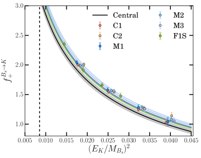
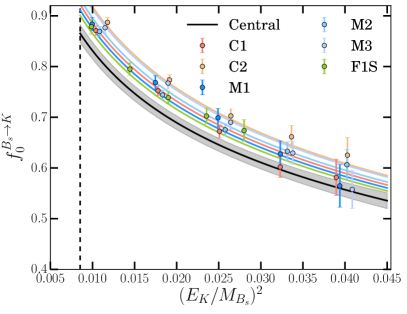
Figure 4: Chiral-continuum extrapolation for the $B_{s}\to K\ell\nu$ form factors $f_{+}$ (left) and $f_{0}$ (right). The colored data points show the underlying data. The colored lines show the result of the fit evaluated at the parameters of the respective ensembles. The gray bands display the obtained form factors in the chiral-continuum limit and the associated statistical uncertainty.

We extrapolate the renormalized lattice form factors to vanishing lattice spacing and to the physical light-quark mass, and interpolate in the kaon energy, using next-to-leading order (NLO) SU(2) chiral perturbation theory for heavy-light mesons (HM$\chi$PT) in the “hard-pion” (or in this case kaon) limit [47, 48, 49]. In the SU(2) theory, the strange quark is integrated out. The chiral logarithms for $B_{s}\to K\ell\nu$ depend on the pion mass and the kaon energy, while the SU(2) low-energy constants depend implicitly on the values of the strange-quark and $b$-quark masses. The function we use is

$$f_{X}^{B_{s}\to K}(M_{\pi},E_{K},a^{2})=\\ \frac{\Lambda}{E_{K}+\Delta_{X}}\left[c_{X,0}\bigg{(}1+\frac{\delta f(M^{s}_{\pi})-\delta f(M^{p}_{\pi})}{(4\pi f_{\pi})^{2}}\bigg{)}\right.\\ \left.+c_{X,1}\frac{\Delta M_{\pi}^{2}}{\Lambda^{2}}+c_{X,2}\frac{E_{K}}{\Lambda}+c_{X,3}\frac{E_{K}^{2}}{\Lambda^{2}}+c_{X,4}(a\Lambda)^{2}\right],$$ (27)

where $X=+,0$ for the vector and scalar form factor, respectively, and where $M_{\pi}^{s}$ is the simulated pion mass on a given ensemble, $M_{\pi}^{p}=(2M_{\pi^{\pm}}+M_{\pi^{0}})/3$ is the isospin-averaged physical pion mass, $\Delta M_{\pi}^{2}=(M_{\pi}^{s})^{2}-(M_{\pi}^{p})^{2}$ and $\Lambda=1\,\text{GeV}$ is the renormalization scale appearing in the one-loop chiral logarithm in $\delta f$ shown in (28) below, and is also used as a dimensionful scale to render the fit coefficients dimensionless. $\Delta_{X}=M_{B^{*}}-M_{B_{s}}$ and the $B^{*}$ is a $\bar{b}u$ flavor state with $J^{P}=1^{-}$ for $f_{+}$, or $J^{P}=0^{+}$ for $f_{0}$. For $f_{+}$ this is the vector meson $B^{*}$ with mass $M_{B^{*}}=5.32471(21)\,\text{GeV}$ [50], while for $f_{0}$ there is a theoretical estimate for the $0^{+}$ state, $M_{B^{*}(0^{+})}=5.63\,\text{GeV}$ [51] (the formalism for effective theories for heavy hadrons of arbitrary spin was derived in Ref. [73] and is reviewed in Ref. [74]). We take $\Delta_{+}=-42.1\,\text{MeV}$ for $f_{+}$ using experimentally-measured masses [50, 75], and $\Delta_{0}=263\,\text{MeV}$ for $f_{0}$ using the theoretical estimate from Ref. [51]. Since the estimated $B^{*}(0^{+})$ pole location is rather far from the physical $q^{2}$ region, the fit is insensitive to its precise position (and varying it is included in our uncertainty for the chiral extrapolation).

While the $0^{+}$ and $1^{-}$ poles describe the physical form factors $f_{0}$ and $f_{+}$, respectively, past work [10, 11] used Eq. (27) for $f_{\|}$ and $f_{\perp}$ based on the observation in Eq. (II.1) that $f_{0}$ is dominated by $f_{\|}$ and $f_{0}$ by $f_{\perp}$. Below we discuss whether this assumption is warranted with our data.

For the case of the $f_{+}$ form factor, the coefficient $c_{3}$ is compatible with zero within statistical errors. Since the quality of the fit remains good when removing this term from the ansatz, we perform the fits for $f_{+}$ without such a term.

The term $\delta f$ entering (27) is the same for $f_{+}$ and $f_{0}$ and is given by

$$\delta f=-\frac{3}{4}\Bigg{(}M_{\pi}^{2}\log\bigg{(}\frac{M_{\pi}^{2}}{\Lambda^{2}}\bigg{)}+\frac{4M_{\pi}}{L}\sum_{|{\bf n}|\neq 0}\frac{K_{1}(|{\bf n}|M_{\pi}L)}{|{\bf n}|}\Bigg{)}.$$ (28)

The first term is the one-loop chiral logarithm and the second term is an estimate for effects due to the finite (spatial) volume, where $K_{1}$ is a modified Bessel function of the second kind and $|{\bf n}|$ is the magnitude of a vector of integers ${\bf n}=(n_{x},n_{y},n_{z})$ specifying the spatial lattice momentum $2\pi{\bf n}/L$. The second term is estimated using one-loop finite-volume SU(2) hard-pion $\chi$PT [76, 77] where loop integrals are replaced by sums over lattice sites, with its expression derived in Ref. [78].

The pion masses entering the fit are obtained from separate two-point correlation function fits and we take $f_{\pi}=130.2\,\text{MeV}$ [79]. We include a term proportional to $a^{2}$ to account for the dominant lattice-spacing dependence. The domain-wall fermion and Iwasaki gluon actions are expected to have discretization errors $O((a\Lambda_{\text{QCD}})^{2})$, about $3\%$ ($5\%$) on the F (M) ensemble(s) for $\Lambda_{\text{QCD}}=500\,\text{MeV}$, while power-counting estimates of errors in the RHQ action and heavy-light current are smaller, below $2\%$. The $a^{2}$ term in our fit therefore accounts for the leading discretization effects.

Results for the parameters of the chiral-continuum fit are given in Table 4. Figure 4 shows the fit, while the systematic errors from variations in the fit are discussed in section IV and shown in Figure 5. Values for the form factors in the continuum and physical quark mass limit, along with their statistical and systematic errors and correlations, are given at the end of the discussion of systematic errors in section IV for a set of reference $q^{2}$ values. These are obtained by using the results in Tab. 4 to evaluate the form factor for a given kaon energy, after setting $a=0$, taking the limit $L\to\infty$ in Eqs. (27) and (28), and setting $m_{\pi}=(2m_{\pi}^{\pm}+m_{\pi}^{0})/3\approx 138$MeV (isospin-averaged pion mass) [50].

Table 4: Fitted parameters for chiral-continuum extrapolation for the $B_{s}\to K\ell\nu$ form factors defined in (27). Results for the coefficients, statistical errors and correlation matrix for the central continuum-limit fit. The fit quality is $(N_{\rm dof}/\chi^{2}_{\rm red.}/p)=(20/1.09/0.35)$ for $f_{+}$ and $(25/1.12/0.11)$ for $f_{0}$.

			$c_{+,0}$	$c_{+,1}$	$c_{+,2}$	$c_{+,4}$	$c_{0,0}$	$c_{0,1}$	$c_{0,2}$	$c_{0,3}$	$c_{0,4}$
	$c^{+,0}$		1.8169	0.2803	-0.7542	-0.0936	0.5310	0.2273	0.2996	-0.0938	-0.0136
		$\delta c^{+,0}$	0.0453	0.2661	0.0411	0.1461	0.0269	0.1057	0.0748	0.0590	0.0567
$c_{+,0}$	1.8169	0.0453	1.0000	-0.3532	-0.6247	-0.4534	0.1671	-0.2710	0.2122	-0.2545	-0.3595
$c_{+,1}$	0.2803	0.2661	-0.3532	1.0000	-0.0280	-0.3974	-0.2226	0.7687	0.0216	-0.0133	-0.2866
$c_{+,2}$	-0.7542	0.0411	-0.6247	-0.0280	1.0000	-0.0035	0.2323	-0.0341	-0.3524	0.4313	0.0124
$c_{+,4}$	-0.0936	0.1461	-0.4534	-0.3974	-0.0035	1.0000	-0.2261	-0.2842	0.0044	-0.0123	0.7535
$c_{0,0}$	0.5310	0.0269	0.1671	-0.2226	0.2323	-0.2261	1.0000	-0.3095	-0.8652	0.8331	-0.2633
$c_{0,1}$	0.2273	0.1057	-0.2710	0.7687	-0.0341	-0.2842	-0.3095	1.0000	0.0950	-0.0942	-0.4221
$c_{0,2}$	0.2996	0.0748	0.2122	0.0216	-0.3524	0.0044	-0.8652	0.0950	1.0000	-0.9836	-0.0143
$c_{0,3}$	-0.0938	0.0590	-0.2545	-0.0133	0.4313	-0.0123	0.8331	-0.0942	-0.9836	1.0000	0.0069
$c_{0,4}$	-0.0136	0.0567	-0.3595	-0.2866	0.0124	0.7535	-0.2633	-0.4221	-0.0143	0.0069	1.0000

IV Systematic error analysis

Our systematic-error analysis has much in common with that done in our earlier work on semileptonic $B\to\pi\ell\nu$ and $B_{s}\to K\ell\nu$ decays [10]. We streamline our discussion where possible, relying on Ref. [10] for details, and introduce new features for this analysis.

Following the same strategy as in Ref. [10], we introduce a set of reference $q^{2}$ values in the range where we have lattice data. By determining the form factors, their statistical uncertainty and all systematic uncertainties at these reference points, we obtain synthetic data points which include the complete and fully correlated error budget. These serve as inputs for the extrapolation over the entire kinematically allowed range $q^{2}\in[0,q^{2}_{\mathrm{max}}]$.

We distinguish between different contributions to the full error budget. The statistical uncertainty is computed from the bootstrap analysis of the chiral and continuum extrapolation described in the previous section III.3. We assess the systematic error arising from these fits in section IV.1 by applying cuts to the data entering the fit as well as varying the functional description of the data, i.e. Eq. (27).

We estimate all remaining sources of uncertainty in sections IV.2 to IV.8. Finally, in section IV.9 we address how to combine these various sources of uncertainty to complete the error budget.

IV.1 Chiral-continuum extrapolation

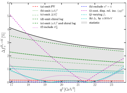
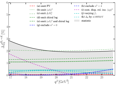
Figure 5: Relative changes, $\Delta f_{X}=|f_{X}^{\text{pref}}-f_{X}^{\text{alt}}|/f_{X}^{\text{pref}}$ for $X=0,+$, of the form-factor central values under variations of the chiral-continuum fit for $B_{s}\to K\ell\nu$. The shaded band shows the statistical uncertainty of the preferred fit.

We estimate the systematic uncertainty from the chiral-continuum extrapolation for $B_{s}\to K\ell\nu$ by performing cuts to the data as well as varying the fit ansatz in Eq. (27). We consider the following variations to the fit form:

1. omitting the finite volume corrections (the second term in $\delta f$),

2. omitting the term proportional to $a^{2}$ ($c_{4}\equiv 0$),

3. omitting the term proportional to $M_{\pi}^{2}$ ($c_{1}\equiv 0$),

4. analytic fits omitting the chiral logarithms ($\delta f\equiv 0$),

5. analytic fits simultaneously omitting the chiral logarithms and the $a^{2}$ term,

6. including the term proportional to $(E_{K}/\Lambda)^{2}$ into the fit for $f_{+}$,

We also vary the data that enters the fit by

1. omitting the data points at the highest momentum, ${\bf p}_{K}=2\pi(2,0,0)/L$ (smallest $q^{2}$),

2. omitting the data points at zero momentum, i.e. $q^{2}_{\text{max}}$ in $f_{0}$,

3. using form factor data that has been obtained by imposing the continuum dispersion relation which at leading order differs from the lattice dispersion relation by powers $(ap)^{2}$. We therefore also include a term $c_{X,5}$ in these fits.

Finally, we consider the impact of variations of some of the numerical values of parameters entering the fit, such as

1. replacing the numerical value of $f_{\pi}$ by its chiral limit value $f_{0}=112\,\text{MeV}$ [20] or by $f_{K}=155.7\,\text{MeV}$ [15],

2. varying the model estimate of $M_{B^{*}(0^{+})}$ entering $\Delta_{0}$ by $\pm 100\,\text{MeV}$ and the experimentally precisely known value of $M_{B^{*}}$ entering $\Delta_{+}$ by a generous $\pm 30\,\text{MeV}$.

Figure 5 shows the relative effects of these variations compared to the statistical uncertainty of the central fit (gray shaded area). We notice that our fit is insensitive to most of these variations. The largest deviations are observed for variations including the lattice spacing and the pion-mass dependence, i.e. variations (b), (c) and (d). However, even these remain of the same size as the statistical errors we quote. We take the largest difference between the preferred fit and any of the alternatives as the systematic uncertainty due to the chiral-continuum extrapolation.

An important subtlety is worth highlighting here. In previous work on the $B_{s}\to K\ell\nu$ semileptonic form factors [10, 11], but also other decay channels like e.g. $B\to\pi\ell\nu$ semileptonic [10, 80], it was assumed that the pole locations of the physical form factors $f_{+}$ and $f_{0}$ also describe the kinematical behaviour of $f_{\perp}$ and $f_{\|}$, respectively. In particular, based on the linear relations in Eqs. (II.1) and (5), $f_{\perp}$ was assumed to be dominated by $f_{+}$ and $f_{\|}$ by $f_{0}$. In Fig. 6 we compare the results when extrapolating the lattice data in both cases using Eq. (27). While with the current level of statistical precision no significant difference is observed for $f_{+}$, a significant difference — which increases with the kaon energy — can be observed for $f_{0}$. Since form-factor parameterizations often rely on the kinematical constraint $f_{+}(0)=f_{0}(0)$, this is a relevant problem for both the vector and scalar form factor. An interesting question in this context is whether this observation could explain the observed tensions between different sets of lattice results for $B_{s}\to K\ell\nu$, as observed by FLAG 21 [15]. Regarding the $B_{s}\to K\ell\nu$ decay we note that HPQCD in Ref. [81] carried out the chiral and continuum limits based on the vector and scalar form factors. In line with our observation their results for $f_{+}$ show a distinctly milder curvature as the results of Ref. [10, 11] (c.f. Fig. 32 in FLAG 21 [15]).

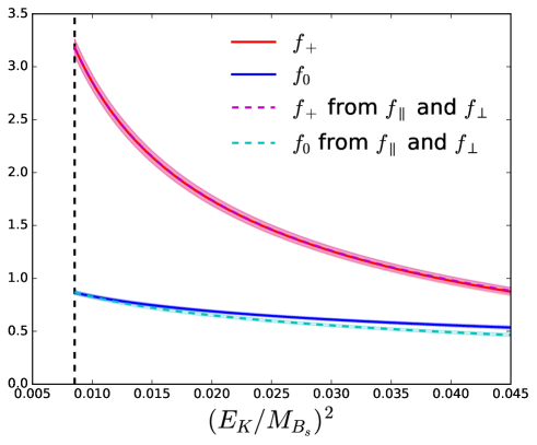
Figure 6: The plot shows the result of the chiral-continuum fit based on Eq. (27), once using $f_{\|}$ and $f_{\perp}$ as input (and subsequently converted to $f_{0}$ and $f_{+}$), and once using $f_{0}$ and $f_{+}$ as input. The results for $f_{0}$ differ significantly and increasingly as the kaon momentum is increased.

IV.2 Lattice-scale uncertainty

We propagate the uncertainty of the lattice-scale determination (c.f. Table 1) by creating a Gaussian distribution with the correct central value and width, which is then used to convert the dimensionless lattice masses into dimensionful quantities prior to the chiral-continuum extrapolations. We therefore do not account separately for this uncertainty.

IV.3 Strange-quark-mass uncertainties

IV.3.1 Valence strange-quark-mass uncertainty

The $B_{s}\to K\ell\nu$ form factors depend explicitly on the valence-strange-quark mass, so the effects of any mistunings in this mass must be accounted for. In order to estimate the corresponding systematic uncertainty, we evaluate the form factors for additional choices of the spectator-quark mass on the C1 ensemble. We determine the fractional change of the form factor with respect to a percentage mistuning in the strange-quark mass, i.e. for $X=+,0$ we compute

$$\Delta f_{X}/\Delta m_{s}\equiv\frac{f_{X}(am_{s})-f_{X}(am^{\mathrm{phys}}_{s})}{am_{s}-am_{s}^{\mathrm{phys}}}\frac{am_{s}^{\mathrm{phys}}}{f_{X}(am^{\mathrm{phys}}_{s})}.$$ (29)

We repeat this for the different choices of momenta and take the largest value this ratio takes, which occurs at the smallest momentum. We tabulate the maximal values of this term for the form factors $f_{+}$ and $f_{0}$ in Table 5. The largest deviation from the physical strange quark mass occurs on the F1S ensemble, where $am_{s}^{\mathrm{sim}}=0.02144$ and $am_{s}^{\mathrm{phys}}=0.02167(20)$. Allowing for one standard deviation we find

$$\Delta m_{s} =\max{\left\{\frac{\left|am_{s}^{\mathrm{sim}}-(am_{s}^{\mathrm{phys}}\pm\delta am_{s}^{\mathrm{phys}})\right|}{am_{s}^{\mathrm{phys}}}\right\}}$$ (30)

$$=1.98\%.$$

Combining this with the above, we determine the maximal deviations as shown in the last line of Table 5. We find that the largest impact of the strange quark mistuning is 0.20% for $f_{+}$ and 0.13% for $f_{0}$ which are far smaller than our leading uncertainties and therefore negligible.

Table 5: Partial derivatives of the form factor as a function of the strange quark mistuning as defined in the text.

	$f_{0}^{B_{s}\to K}$	$f_{+}^{B_{s}\to K}$
$\Delta f_{X}/\Delta m_{s}$	0.0630(46)	0.1027(84)
$\mathrm{max}(\Delta m_{s})\,[\%]$	1.98	1.98
$\mathrm{max}(\Delta f_{X})\,[\%]$	0.13	0.20

IV.3.2 Strange-sea-quark mistuning

Our fit functions do not depend explicitly on the strange sea-quark mass and, at each lattice spacing, we have form factors for only a single value of this mass. We estimate any systematic effects stemming from the sea strange-quark mistuning (which is largest on the coarse ensembles) in the same way, but including an additional suppression factor of $\alpha_{s}$. Numerically, this is approximately $\Delta f_{X}/\Delta m_{s}\times\alpha_{s}\times\max(\Delta m^{\mathrm{sea}}_{s})=0.28\%$ and $0.46\%$ for $f_{0}$ and $f_{+}$, respectively. This is intended as a conservative estimate for this uncertainty and it is a negligible contribution to the total error budget.

IV.4 Effects of the RHQ parameter uncertainty on the form factors

As outlined in appendix A, the RHQ tuning procedure determines three coefficients in the RHQ action. These are the bare $b$-quark mass ($m_{0}a$), the clover coefficient ($c_{P}$) and the anisotropy ($\zeta$). The experimental inputs to this tuning are the measured $B_{s}$-meson mass and the hyperfine splitting ($\Delta M_{B_{s}}\equiv M_{B_{s}^{*}}-M_{B_{s}}$). In addition, the lattice scale and the physical strange-quark mass are required inputs. Furthermore, we enforce that the rest mass equals the kinetic mass. The tuned parameters, including estimates for all relevant sources of uncertainties are listed in Table 17 in appendix A.

In order to propagate the effect of these tuning uncertainties onto the form factors, we generated additional form factor data for different choices of the RHQ parameters on the C1 ensemble. Using this data set we determine the partial derivatives of the form factors with respect to the respective RHQ parameters. We normalize these values by the ratio of the tuned form factor and respective RHQ parameters on this ensemble and conservatively quote the maximum value this takes. These values are listed in the first two rows of Table 6.

Table 6: Estimates for the normalized partial derivatives on the C1 ensemble (top two rows) and the maximum uncertainty propagated onto the form factors.

	$am_{0}$	$\zeta$	$c_{P}$
$f_{+}$ max normalized slope	0.2368	0.1003	0.0543
$f_{0}$ max normalized slope	0.1067	0.0418	0.1089
$f_{+}$ RHQ uncertainty $[\%]$	0.8145	0.9004	0.3215
$f_{0}$ RHQ uncertainty $[\%]$	0.3670	0.3755	0.6448

We derive the uncertainty on the form factor due to a given RHQ parameter by multiplying these normalized derivatives on the C1 ensemble with the relative uncertainty of this RHQ parameter on a given lattice spacing. We illustrate this on the example of $\zeta$

$$\left(\frac{\delta f_{X}}{f^{\mathrm{tuned}}_{X}}\right)_{\zeta}=\max_{{\bf n}}\left(\frac{\zeta^{\mathrm{tuned}}}{f_{X}^{\mathrm{tuned}}}\frac{\partial f_{X}}{\partial\zeta}\right)\Bigg{|}_{C1}\frac{\delta\zeta}{\zeta^{\mathrm{tuned}}}\,,$$ (31)

where $f_{X}^{\mathrm{tuned}}$ is the form factor evaluated at the tuned value of the RHQ parameters on C1, whilst the last term is evaluated lattice spacing-by-lattice spacing.

We find that the uncertainty is largest on the F1S ensemble and therefore take this to provide a conservative estimate for the RHQ parameter tuning on the form factors and list their values in the last two rows of Table 6. Adding these contributions in quadrature we quote an uncertainty of $1.26\%$ on $f_{+}$ and $0.83\%$ on $f_{0}$.

IV.5 Discretization errors

Due to their different origin and size, we separately discuss discretization errors due to the light quarks and gluons in the action, the heavy-light current, and the RHQ quarks.

IV.5.1 Discretization effects from the action and the current

The dominant discretization error from the light quarks and gluons in the action is $O((a\Lambda_{\text{QCD}})^{2})$ which, using $\Lambda_{\text{QCD}}=500\,\text{MeV}$, amounts to $\sim 3.2\%$ on the finest ensemble. This is accounted for by including $a^{2}$-terms in the chiral-continuum extrapolations. We assign the estimate $(a\Lambda_{\text{QCD}})^{4}\sim 0.10\%$ for subsequent terms. Potential uncertainties stemming from the residual chiral symmetry breaking are estimated to be of the size $am_{\text{res}}\sim 0.1\%$ for the light quarks.

The leading quark and gluon discretization errors in the heavy-light currents are $O(\alpha_{s}a\tilde{m}_{l},(a\tilde{m}_{l})^{2},\alpha_{s}^{2}a\Lambda_{\text{QCD}},(ap)^{2})$.

In the comparison between our central fit and the variations (i) and (g), we do not observe any evidence of sizable momentum-dependent discretization errors in our data. Thus we do not include a systematic error from this source.

Estimating the effects by power counting on the fine ensemble, the first two terms are negligible ($<0.1\%$), while the third amounts to $\sim 0.78\%$. Combining this in quadrature with the $(a\Lambda_{\text{QCD}})^{4}$ and $am_{\text{res}}$ from above, we quote 0.79%.

IV.5.2 Heavy quark discretization errors

The RHQ action gives rise to nontrivial lattice-spacing dependence in the form factors when $m_{0}a\sim 1$. To estimate the resulting discretization errors, we use the same power-counting approach as in our previous papers [33, 38, 10]. For reproducibility and completeness we provide a brief summary of the procedure as well as intermediate numerical values in Appendix B. We take the size of heavy-quark discretization errors in our calculation of semileptonic form factors from the estimate on our finest ensemble ($a^{-1}=2.785\,\text{GeV}$). They amount to $\sim 1.3\%$ for the lattice form factor $f_{\|}$ and $\sim 1.5\%$ for $f_{\perp}$.

IV.6 Renormalization factor

The renormalization factor relating the lattice weak current to the continuum one is shown in Eq. (8) in section II.3, where $Z_{V_{\mu}}^{bl}$ is given by a product of three components. We consider the uncertainties from these three multiplicative factors separately, and add them in quadrature to obtain the total error on the form factors.

For $Z_{V}^{ll}$, we use the non-perturbatively-determined value of the axial-current renormalization factor $Z_{A}$ evaluated at the value of the light quark mass (see table 2 for numerical values). We can neglect the statistical uncertainty in $Z_{A}$ (which is only $0.02\%$ on the finer ensembles) and the difference between $Z_{V}^{ll}$ and $Z_{A}$ (which is $O(am_{\text{res}})\sim 7\times 10^{-4}$ at $a\approx 0.086\,\text{fm}$).

For $Z_{V}^{bb}$, we use the non-perturbative determination from Ref. [38]. The statistical uncertainty in $Z_{V}^{bb}$ on the finer ensemble is well below one percent and propagated into the statistical error analysis. The perturbative truncation error in $\rho_{V}^{bl}$ is taken to be the full size of the 1-loop correction at the finer $a\approx 0.086\,\text{fm}$ lattice spacing, which leads to $1.7$% for $\rho_{V_{0}}$ and $0.6$% for $\rho_{V_{i}}$. We use the values of $\rho_{V_{\mu}}$ and $Z_{V}^{ll}$ in the chiral limit and must consider errors due to the nonzero physical up, down, and strange masses. The leading quark-mass dependent errors in $\rho_{V_{\mu}}$ and $Z_{V}^{ll}$ are $O(\alpha_{s}a\tilde{m}_{q})$ and $O((a\tilde{m}_{q})^{2})$, respectively, but these are already accounted for in our estimate of light-quark and gluon discretization errors (see Sec. IV.5.1) and we do not count them again here.

Perturbative truncation errors are by far the dominant source of uncertainty in the renormalization factor, and the quadrature sum of the three error contributions is $1.7\%$ for $f_{\|}$ and 0.6% for $f_{\perp}$.

IV.7 Finite-volume corrections

As discussed in section III.3, we directly account for the finite size effects in the chiral continuum extrapolation (i.e. in Eq. (27)). We can assess the numerical size of these effects by comparing to a fit that does not include the second term in Eq. (28). The maximum deviation for $f_{0}$ ($f_{+}$) is given by 0.06% (0.13%).

IV.8 Isospin breaking

The leading quark-mass contribution to the isospin breaking from the valence-quark masses is of $O((m_{d}-m_{u})/\Lambda_{\text{QCD}})\sim 0.5\%$, obtained using $m_{d}-m_{u}=2.38(18)\,\text{MeV}$ [82] and $\Lambda_{\text{QCD}}=500\,\text{MeV}$. The difference between the $u$ and $d$ quark masses in the sea sector should have a negligible effect on the form factors because the sea quarks couple to the valence quarks through $I=0$ gluon exchange, giving an uncertainty of $O(((m_{d}-m_{u})/\Lambda_{\text{QCD}})^{2})\sim 0.003\%$. The electromagnetic contribution to isospin breaking is expected to be $O(\alpha_{QED})\sim 1/137=0.7\%$. We therefore take $0.7\%$ as the uncertainty from isospin breaking and electromagnetic effects.

IV.9 Form factor results and correlation matrices

Table 7: Values and error budgets for the $B_{s}\to K\ell\nu$ form factors at three representative $q^{2}$ values in the range of simulated lattice momenta. The total error is obtained by adding the individual errors in quadrature. See Tab. 8 for the corresponding correlation matrices. The data shown in this table is contained in the accompanying data file.

	$f_{+}$		$f_{0}$
$q^{2}[{\rm GeV}^{2}]$	17.60	23.40	17.60	20.80	23.40
$f_{+,0}(q^{2})$	0.9878	2.9301	0.5594	0.6843	0.8397
Error budget (absolute contribution)
Statistical error	0.0377	0.0743	0.0141	0.0133	0.0167
Chiral-continuum extrapol.	0.0407	0.0698	0.0116	0.0139	0.0180
Other	0.0240	0.0700	0.0139	0.0172	0.0213
Total	0.0604	0.1236	0.0230	0.0258	0.0325
Error budget (in per cent)
Statistical error	3.82	2.54	2.53	1.94	1.99
Chiral-continuum extrapol.	4.12	2.38	2.06	2.03	2.14
Other	2.43	2.39	2.49	2.51	2.54
Total	6.12	4.22	4.10	3.77	3.87

Table 8: Statistical, fit- and flat-systematic errors $\delta f_{+/0}$ for representative $q^{2}$ values (given in units of GeV² as arguments of $f_{+/0}$), and corresponding correlation matrices. The data shown in this table is contained in the accompanying data file.

			$f_{+}$		$f_{0}$
	$q^{2}\,[{\rm GeV}^{2}]$		$17.60$	$23.40$	$17.60$	$20.80$	$23.40$
		$\delta f_{+/0}$	0.0377	0.0743	0.0141	0.0133	0.0167
$f_{+}$	$17.60$	0.0377	1.0000	0.8254	0.6976	0.7540	0.7212
	$23.40$	0.0743	0.8254	1.0000	0.5165	0.7632	0.8008
$f_{0}$	$17.60$	0.0141	0.6976	0.5165	1.0000	0.8118	0.7117
	$20.80$	0.0133	0.7540	0.7632	0.8118	1.0000	0.9699
	$23.40$	0.0167	0.7212	0.8008	0.7117	0.9699	1.0000

statistical

			$f_{+}$		$f_{0}$
	$q^{2}\,[{\rm GeV}^{2}]$		$17.60$	$23.40$	$17.60$	$20.80$	$23.40$
		$\delta f_{+/0}$	0.0407	0.0698	0.0116	0.0139	0.0180
$f_{+}$	$17.60$	0.0407	1.0000	0.8254	0.6976	0.7540	0.7212
	$23.40$	0.0698	0.8254	1.0000	0.5165	0.7632	0.8008
$f_{0}$	$17.60$	0.0116	0.6976	0.5165	1.0000	0.8118	0.7117
	$20.80$	0.0139	0.7540	0.7632	0.8118	1.0000	0.9699
	$23.40$	0.0180	0.7212	0.8008	0.7117	0.9699	1.0000

fit systematic

			$f_{+}$		$f_{0}$
	$q^{2}\,[{\rm GeV}^{2}]$		$17.60$	$23.40$	$17.60$	$20.80$	$23.40$
		$\delta f_{+/0}$	0.0240	0.0700	0.0139	0.0172	0.0213
$f_{+}$	$17.60$	0.0240	1.0000	0.9974	0.9461	0.9419	0.9368
	$23.40$	0.0700	0.9974	1.0000	0.9229	0.9178	0.9115
$f_{0}$	$17.60$	0.0139	0.9461	0.9229	1.0000	0.9999	0.9995
	$20.80$	0.0172	0.9419	0.9178	0.9999	1.0000	0.9998
	$23.40$	0.0213	0.9368	0.9115	0.9995	0.9998	1.0000

flat systematic

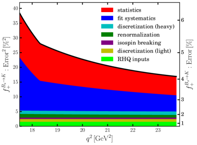
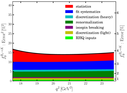
Figure 7: Cumulative systematic errors for the chiral- and continuum-extrapolated form factor for $B_{s}\to K\ell\nu$.

In the next section we will fit a $z$-expansion to synthetic data for the physical form factors in the continuum and infinite-volume limit, generated at selected values of $q^{2}$, to extend our form factors to the full kinematic range. Because we first extrapolate to the continuum limit and then perform the z-expansion to extend the form factors over the full kinematic range, the number of available independent reference $q^{2}$ values is restricted by the number of resolved parameters in the chiral-continuum limit of the HM$\chi$PT description of the lattice data. Since we resolve 3 (2) parameters that parameterize the continuum form factors $f_{0}$ ($f_{+}$), the number of synthetic data points we can choose is limited by this. We account for the correlations between the form factors at these $q^{2}$ values as follows.

The total error budget can be divided into three major contributions: the statistical uncertainty, the uncertainties associated to the chiral-continuum extrapolation and the uncertainties that are estimated as a constant $q^{2}$ independent percentage of the form factors. We refer to these as statistical, fit systematic and flat systematic. Whilst most of the latter are estimated as a percentage uncertainty on the form factors $f_{+}$ and $f_{0}$, the contributions described in Secs. IV.5.2 and IV.6 are determined with respect to the form factors $f_{\parallel}$ and $f_{\perp}$, which induces a mild $q^{2}$ dependence when this is related to $f_{+}$ and $f_{0}$. The resulting cumulative systematic errors for $B_{s}\to K\ell\nu$ are illustrated in Fig. 7. We now provide more detail on estimating the correlations of the different sources of uncertainties at the reference values.

It is straightforward to obtain the statistical correlations from the bootstrap analysis of the chiral and continuum fit in Sec. III.3.

The systematic error for the chiral-continuum extrapolation is found by varying the fit function and parametric inputs, as described above. This does not provide information on correlations between different $q^{2}$-values. However, alternate chiral-continuum fits with different fit functions exhibit very similar statistical correlations between $q^{2}$-bins. Hence we take the statistical correlation matrix from our preferred fit and multiply it by the estimated chiral-continuum extrapolation error at each $q^{2}$ value. For off-diagonal elements of the correlation matrix we use the product $\sigma_{q^{2}_{i}}\sigma_{q^{2}_{j}}$.

We assume each of the remaining “flat” systematic errors to be $100\%$ correlated and add the corresponding covariance matrices. Where the per-cent error is given for $f_{\|}$ and $f_{\perp}$, we first construct the corresponding covariance matrix for $f_{\|}$ and $f_{\perp}$ and then propagate the correlated error in order to obtain the covariance matrix for $f_{+}$ and $f_{0}$. Table 8 shows the resulting statistical and systematic correlation matrices, which enable the full reconstruction of the total covariance matrices using the form factor values and errors from table 7.

V Phenomenological applications

V.1 $z$-expansions of form factors

Once we have continuum values for the form factors, we extrapolate them over the entire physical range of $q^{2}$ using a fit to a $z$-expansion [83, 84, 85, 86, 87, 88, 89, 90]. The squared momentum transfer, $q^{2}$, is mapped to the variable $z$ using

$$z(q^{2};t_{*},t_{0})=\frac{\sqrt{t_{*}-q^{2}}-\sqrt{t_{*}-t_{0}}}{\sqrt{t_{*}-q^{2}}+\sqrt{t_{*}-t_{0}}}\,.$$ (32)

This transformation maps the complex $q^{2}$ plane, with a cut for $q^{2}\geq t_{*}$, onto the unit disk in $z$. For use below we set $t_{\pm}=(M_{B_{s}}\pm M_{K})^{2}$, with $t_{-}=q^{2}_{\text{max}}$, while $t_{*}$ is fixed by the appropriate two-particle production threshold $t_{*}=(M_{B}+M_{\pi})^{2}$. The value of $t_{0}$ can be chosen to fix the range in $z$ corresponding to a given range in $q^{2}$. We choose

$$t_{0}=t_{\mathrm{opt}}=t_{*}-\sqrt{t_{*}(t_{*}-t_{-})}\,.$$ (33)

This symmetrizes the range of $z$ about zero for $0\leq q^{2}\leq q^{2}_{\text{max}}$ which is mapped onto the real axis $0.2\gtrsim z\gtrsim-0.2$, indicating that an expansion of the form factor in $z$ rather than in $q^{2}$ might converge quickly. This motivated Boyd, Grinstein and Lebed (BGL) [84] to write the form factor as

$$f_{X}(q^{2})=\frac{1}{B_{X}(q^{2})\phi_{X}(q^{2},t_{0})}\sum_{n\geq 0}a_{X,n}(t_{0})z^{n},$$ (34)

where $\phi_{X}(q^{2},t_{0})$ is known as the outer function, with expressions given in Appendix D. For $X=+,0$, the Blaschke factor $B_{X}(q^{2})$ is chosen to vanish at the positions of sub-threshold poles $M^{X}_{i}$,

$$B_{X}(q^{2})=\prod\limits_{i\in X\,{\rm poles}}z\left(q^{2};t_{\ast},\left(M^{X}_{i}\right)^{2}\right)\,.$$ (35)

For $f_{+}$ the measured $1^{-}$ vector-meson with $M^{+}_{B^{\ast}(1^{-})}=5.32471\,\text{GeV}$ [50] sits above the physical semileptonic region $0\leq q^{2}\leq q^{2}_{\rm max}$, but also below the $B\pi$ threshold. Specifically, $q^{2}_{\rm max}\leq(M^{+}_{B^{\ast}(1^{-})})^{2}\leq t_{\ast}\to 23.73\,\text{GeV}^{2}\leq 28.35\,\text{GeV}^{2}\leq 29.35\,\text{GeV}^{2}$ . We cancel this pole through the corresponding Blaschke factor $B_{+}(q^{2})$ prior to expanding in $z$. For $f_{0}$ the theoretically predicted pole mass $M^{0}_{B^{\ast}(0^{+})}=5.63\,\text{GeV}$ [51] sits above the $B\pi$ threshold and no pole needs to be cancelled.

The following unitarity constraint applies:

$$\frac{1}{2\pi i}\oint_{C}\frac{dz}{z}\theta_{z}|B_{X}(q^{2})\phi_{X}(q^{2},t_{0})f_{X}(q^{2})|^{2}\leq 1\,,$$ (36)

with $C$ the unit circle, $\theta_{z}\equiv\theta(\alpha_{B_{s}K}-|{\rm arg}[z]|)$ and $\alpha_{B_{s}K}={\rm arg}[z(t_{+},t_{\ast},t_{0})]$. Since for the $B_{s}\to K\ell\nu$ transition the two-particle $B\pi$ production threshold lies below the $B_{s}K$ threshold, i.e. $t_{\ast}<t_{+}$, the unitarity constraint originally proposed by BGL [84] needs to be modified. This is similar to the situation discussed in Refs. [91, 92, 93, 94], but note some differences in notation in those papers, in particular our use of $t_{\ast}$ and $t_{+}$ for the locations of the $B\pi$ and $B_{s}K$ production thresholds, respectively. The step function $\theta_{z}$ achieves this by restricting the integration over the unit circle to the relevant arc. Let us now define the inner product

$$\langle z^{i}|z^{j}\rangle_{\alpha} =\frac{1}{2\pi}\int\limits_{-\alpha}^{\alpha}d\phi(z^{i})^{\ast}z^{j}|_{z=e^{i\phi}}\,,$$ (37)

$$=\begin{cases}\displaystyle\frac{\sin(\alpha(i-j))}{\pi(i-j)}&i\neq j\\ \displaystyle\frac{\alpha}{\pi}&i=j\end{cases}$$

on the arc $[-\alpha,+\alpha]$ of the unit circle. When the inner product is defined over the entire unit circle, $[-\pi,+\pi]$, the monomials $z^{i}$ are orthonormal, $\langle z^{i}|z^{j}\rangle_{\pi}=\delta_{ij}$. In that case the unitarity constraint Eq. (36) becomes $\sum_{i}|a_{X,i}|^{2}\leq 1$. With the restriction to the arc $[-\alpha_{B_{s}K},+\alpha_{B_{s}K}]$, the modified BGL unitarity constraint developed in [95] is

$$\sum\limits_{i,j\geq 0}a_{X,i}^{\ast}\langle z^{i}|z^{j}\rangle_{\alpha_{B_{s}K}}a_{X,j}\equiv|{\bf a}_{X}|_{\alpha_{B_{s}K}}^{2}\leq 1\,,$$ (38)

where we have defined $|{\bf a}_{X}|_{\alpha_{B_{s}K}}^{2}$ to mean the quadratic form on the left-hand side.

V.2 Extrapolation to $q^{2}=0$

To extrapolate our results to the full physical range of $q^{2}$ we start from the results for $f_{+}$ and $f_{0}$ listed in Tab. 7, with statistical and systematic errors and correlations given in Tab. 8, added in quadrature. Input parameters for the $z$ fits are summarized in Tab. 9. We use the short-hand vector notation ${\bf f}=({\bf f}_{+},{\bf f}_{0})^{T}$ for the vector and scalar form factors at the kinematical reference points, and denote the corresponding covariance matrix by $C_{\bf f}$. We fit the data to a $z$-parameterization of Eq. (34), subject to the unitarity constraint Eq. (38) and the kinematical constraint $f_{+}(0)=f_{0}(0)$.

Table 9: Input masses for the BGL $z$ fits. Values are in GeV [50]. The superscript $\dagger$ indicates, where the isospin-averaged mass has been taken.

$M_{B}$	$M_{B_{s}}$	$M_{\pi}$	$M_{K}$	$M^{+}_{B^{\ast}(0^{+})}$
$5.27950^{\dagger}$	$5.36682$	$0.138039^{\dagger}$	$0.495644^{\dagger}$	5.32471

In the Bayesian-inference strategy for fitting form factors developed in Ref. [95] the unitarity constraint is implemented as a flat prior, which acts as a regulator for the fitting problem. In contrast to frequentist fits, this allows us to determine the parameters of a BGL parameterization to arbitrarily high order, removing errors from truncating the power series in $z$ in Eq. (34).

The Bayesian-inference problem of determining the BGL parameters ${\bf a}=({\bf a}_{+},{\bf a}_{0})^{T}$ and functions $g({\bf a})$ of them amounts to computing expectation values

$$\langle g({\bf a})\rangle=\mathcal{N}\int d{\bf a}\,g({\bf a})\,\pi({\bf a}|{\bf f},C_{\bf f})\pi_{\bf a}\,,$$ (39)

where $\mathcal{N}$ is a normalization constant. As prior knowledge on the form factor we use only the unitarity constraint expressed in terms of the distribution

$$\pi_{\bf a}\propto\theta\left(1-|{\bf a}_{+}|_{\alpha_{B_{s}K}}^{2}\right)\theta\left(1-|{\bf a}_{0}|_{\alpha_{B_{s}K}}^{2}\right)\,,$$ (40)

which essentially limits the integration range in Eq. (39). The conditional probability density for the parameter ${\bf a}$ given the fit model and data is

$$\pi({\bf a}|{\bf f},C_{{\bf f}}) \propto{\rm exp}\left(-\frac{1}{2}\chi^{2}({\bf a},{\bf f})\right)\,,$$ (41)

where

$$\chi^{2}({\bf a},{\bf f})=({\bf f}-Z{\bf a})^{T}C_{{\bf f}}^{-1}({\bf f}-Z{\bf a})\,.$$ (42)

Following Ref. [95], the matrix $Z$ consists of diagonal blocks

$$(Z_{XX})_{ij}=\frac{z^{j}}{B_{X}(q_{i}^{2})\phi_{X}(q_{i}^{2},t_{0})},$$ (43)

where $XX$ is either $++$ or $00$, for the vector and scalar form factors, respectively. The off-diagonal blocks, which implement the kinematical constraint $f_{+}(0)=f_{0}(0)$ are

$$(Z_{+0})_{ij}= 0\,,$$

$$(Z_{0+})_{ij}= \frac{1}{z(0;t_{\ast},M_{B^{\ast}}^{2})\phi_{+}(0)}\frac{\phi_{0}(0)}{\phi_{0}(q_{i}^{2})}z^{j}(0)\,.$$

The integral in Eq. (39) can be performed by Monte Carlo, which corresponds to drawing multi-variate normal-distributed pseudo-random numbers. An efficient algorithm and an implementation in Python are presented in Refs. [95, 96]. The results presented here are based on 2000 samples.

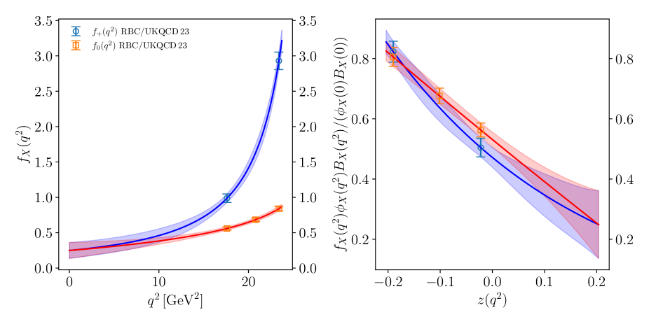
Figure 8: $z$-fits to $B_{s}\to K\ell\nu$ form factors for $(K_{+},K_{0})=(5,5)$, plotted against $q^{2}$ (left) and against $z$ (right), where in the latter plot the outer function and Blaschke factor have been removed. Blue denotes $f_{+}$ and red $f_{0}$.

Figure 8 shows the results of $z$-fits to our $B_{s}\to K\ell\nu$ data, with numerical values for the fit parameters in table 10.

For the discussion of the results it is also worthwhile, in parallel, to have a look at the first data column of Tab. 11, which shows the result for the form factor extrapolated to $q^{2}=0$. For both the coefficients ${\bf a}$ and $f_{+}(0)$ we find significant variation in both error and central value when increasing the order of the $z$ expansion from $K_{+,0}=2$. We find stable central values and errors for $K\geq 3$. Higher-order coefficients can be added to the fit (the tables show results up to $K_{+,0}=10$), whereby the errors on the significantly-determined lower-order coefficients and also the result for $f_{+,0}(0)$ remain stable, and the higher-order coefficients are compatible with zero. We conclude that the form factor parameterization determined in this way becomes truncation independent for large-enough $K_{+,0}$. For the following analyses we use results with $(K_{+},K_{0})=(5,5)$.

Furthermore, the value of the form factors at $q^{2}=0$ is of interest for comparison with predictions from different theoretical methods. Using light cone sum rules, Duplancic/Melic report $f(0)=0.30(^{+4}_{-3})$ [97] and Khodjamirian/Rusov quote $f(0)=0.336(23)$ [98]. Based on a relativistic quark model Faustov/Galkin predict $f(0)=0.284(14)$ [99], where the NLO perturbative-QCD result by Wang/Xiao is $f(0)=0.26(^{+4}_{-3})(2)$ [100]. All these values are compatible with our $(K_{+},K_{0})=(5,5)$ result

$$f(q^{2}=0)=0.25(11),$$ (45)

however, our uncertainty at $q^{2}=0$ is substantially larger than for these other predictions.

Table 10: Results for $z$-fits to data for scalar and vector form factors for $B_{s}\to K\ell\nu$. The main results of this paper are the ones with $(K_{+},K_{0})=(5,5)$. The data for this case and the corresponding correlation matrix is contained in the accompanying data file.

$K_{+}$	$K_{0}$	$a_{+,0}$	$a_{+,1}$	$a_{+,2}$	$a_{+,3}$	$a_{+,4}$	$a_{+,5}$	$a_{+,6}$	$a_{+,7}$	$a_{+,8}$	$a_{+,9}$
2	2	0.0293(11)	-0.0871(46)	-	-	-	-	-	-	-	-
2	3	0.0249(16)	-0.0999(57)	-	-	-	-	-	-	-	-
3	2	0.0245(16)	-0.0799(50)	0.093(21)	-	-	-	-	-	-	-
3	3	0.0245(15)	-0.078(12)	0.101(49)	-	-	-	-	-	-	-
3	4	0.0246(16)	-0.078(16)	0.100(70)	-	-	-	-	-	-	-
4	3	0.0246(17)	-0.075(31)	0.102(49)	-0.07(72)	-	-	-	-	-	-
4	4	0.0246(17)	-0.077(32)	0.100(68)	-0.03(70)	-	-	-	-	-	-
5	5	0.0246(17)	-0.074(31)	0.099(70)	-0.08(67)	0.05(70)	-	-	-	-	-
6	6	0.0247(16)	-0.073(32)	0.101(69)	-0.10(69)	0.09(74)	-0.05(71)	-	-	-	-
7	7	0.0247(17)	-0.071(33)	0.107(70)	-0.11(72)	0.08(89)	-0.04(89)	0.03(73)	-	-	-
8	8	0.0248(17)	-0.068(35)	0.102(74)	-0.18(77)	0.2(1.1)	-0.2(1.3)	0.1(1.2)	-0.06(82)	-	-
9	9	0.0248(18)	-0.068(38)	0.107(85)	-0.16(82)	0.2(1.4)	-0.2(1.9)	0.1(1.9)	-0.1(1.5)	0.03(89)	-
10	10	0.0247(18)	-0.067(43)	0.112(95)	-0.15(90)	0.2(1.8)	-0.2(2.6)	0.1(2.9)	-0.1(2.7)	-0.0(1.9)	0.02(98)

$K_{+}$	$K_{0}$	$a_{0,0}$	$a_{0,1}$	$a_{0,2}$	$a_{0,3}$	$a_{0,4}$	$a_{0,5}$	$a_{0,6}$	$a_{0,7}$	$a_{0,8}$	$a_{0,9}$
2	2	0.0981(36)	-0.286(14)	-	-	-	-	-	-	-	-
2	3	0.0917(39)	-0.331(19)	-0.211(53)	-	-	-	-	-	-	-
3	2	0.0950(37)	-0.263(15)	-	-	-	-	-	-	-	-
3	3	0.0953(43)	-0.254(41)	0.02(13)	-	-	-	-	-	-	-
3	4	0.0955(44)	-0.254(42)	0.02(22)	-0.02(60)	-	-	-	-	-	-
4	3	0.0954(43)	-0.254(40)	0.03(12)	-	-	-	-	-	-	-
4	4	0.0953(42)	-0.254(42)	0.02(21)	-0.02(60)	-	-	-	-	-	-
5	5	0.0954(44)	-0.254(41)	0.02(21)	-0.01(55)	-0.00(62)	-	-	-	-	-
6	6	0.0957(42)	-0.251(41)	0.04(21)	-0.01(52)	-0.06(65)	0.07(65)	-	-	-	-
7	7	0.0955(44)	-0.250(40)	0.06(20)	0.05(50)	-0.13(72)	0.17(79)	-0.12(69)	-	-	-
8	8	0.0954(43)	-0.250(41)	0.06(22)	0.06(50)	-0.18(84)	0.2(1.0)	-0.21(99)	0.10(74)	-	-
9	9	0.0956(44)	-0.247(41)	0.08(23)	0.06(50)	-0.27(96)	0.4(1.4)	-0.4(1.5)	0.3(1.2)	-0.15(80)	-
10	10	0.0956(42)	-0.245(42)	0.11(24)	0.11(49)	-0.4(1.1)	0.7(1.8)	-0.8(2.2)	0.7(2.1)	-0.4(1.5)	0.16(87)

Table 11: Results for observables based on the results for the $z$ fits in Tab. 10. The main results of this paper are the ones with $(K_{+},K_{0})=(5,5)$.

$K_{+}$	$K_{0}$	$f(q^{2}=0)$	$R_{B_{s}\to K}^{\rm impr}$	$R_{B_{s}\to K}$	$\frac{\Gamma^{\tau}}{|V_{ub}|^{2}}\,[\frac{1}{\rm ps}]$	$\frac{\Gamma^{\mu}}{|V_{ub}|^{2}}\,[\frac{1}{\rm ps}]$	$V^{\rm low}_{\rm CKM}$	$V^{\rm high}_{\rm CKM}$	$V^{\rm full}_{\rm CKM}$
2	2	0.222(21)	1.545(17)	0.741(19)	5.37(43)	7.25(70)	0.00356(39)	0.00325(30)	0.00336(32)
2	3	0.087(39)	1.657(46)	0.954(75)	3.70(50)	3.94(81)	0.0070(22)	0.00408(46)	0.00420(52)
3	2	0.231(21)	1.721(57)	0.774(27)	4.34(45)	5.62(72)	0.00375(42)	0.00382(41)	0.00379(39)
3	3	0.248(88)	1.721(56)	0.76(10)	4.48(72)	6.1(1.7)	0.0039(14)	0.00381(46)	0.00381(52)
3	4	0.25(12)	1.722(64)	0.77(15)	4.51(84)	6.2(2.3)	0.0042(22)	0.00380(48)	0.00382(53)
4	3	0.249(86)	1.72(12)	0.76(12)	4.55(82)	6.3(2.0)	0.0039(16)	0.00378(53)	0.00379(59)
4	4	0.25(12)	1.72(12)	0.78(17)	4.53(89)	6.3(2.4)	0.0043(29)	0.00381(57)	0.00383(62)
5	5	0.25(11)	1.72(11)	0.77(16)	4.57(90)	6.4(2.4)	0.0041(24)	0.00376(55)	0.00378(61)
6	6	0.26(11)	1.71(11)	0.76(16)	4.63(88)	6.5(2.4)	0.0040(26)	0.00375(54)	0.00376(58)
7	7	0.26(11)	1.71(11)	0.75(15)	4.67(90)	6.7(2.4)	0.0038(19)	0.00373(56)	0.00374(62)
8	8	0.26(11)	1.70(12)	0.74(15)	4.71(94)	6.8(2.6)	0.0038(19)	0.00371(55)	0.00372(62)
9	9	0.27(11)	1.70(12)	0.74(16)	4.76(98)	7.0(2.7)	0.0038(20)	0.00370(59)	0.00371(66)
10	10	0.28(11)	1.71(13)	0.73(16)	4.80(99)	7.1(2.8)	0.0037(31)	0.00368(58)	0.00368(62)

Table 12: Results for observables based on the results for the $z$ fits in Tab. 10. The main results of this paper are the ones with $(K_{+},K_{0})=(5,5)$.

$K_{+}$	$K_{0}$	$I[\mathcal{A}_{\rm FB}^{\tau}]\,[\frac{1}{\rm ps}]$	$I[\mathcal{A}_{\rm FB}^{\mu}]\,[\frac{1}{\rm ps}]$	$\mathcal{\bar{A}}_{\rm FB}^{\tau}$	$\mathcal{\bar{A}}_{\rm FB}^{\mu}$	$I[\mathcal{A}_{\rm pol}^{\tau}]\,[\frac{1}{\rm ps}]$	$I[\mathcal{A}_{\rm pol}^{\mu}]\,[\frac{1}{\rm ps}]$	$\mathcal{\bar{A}}_{\rm pol}^{\tau}$	$\mathcal{\bar{A}}_{\rm pol}^{\mu}$
2	2	1.46(12)	0.0320(46)	0.2720(21)	0.00440(27)	0.794(92)	7.16(68)	0.148(13)	0.98768(73)
2	3	0.99(14)	0.0115(41)	0.2679(27)	0.00284(46)	0.31(13)	3.90(80)	0.082(27)	0.9912(11)
3	2	1.23(13)	0.0315(46)	0.2825(28)	0.00560(44)	0.14(15)	5.53(71)	0.031(34)	0.9838(13)
3	3	1.27(23)	0.038(19)	0.2836(77)	0.0058(15)	0.13(16)	6.0(1.7)	0.030(35)	0.9833(39)
3	4	1.28(27)	0.040(26)	0.2833(91)	0.0057(19)	0.14(17)	6.1(2.2)	0.030(38)	0.9834(49)
4	3	1.29(26)	0.038(19)	0.2820(80)	0.0058(16)	0.18(31)	6.2(2.0)	0.034(65)	0.9832(45)
4	4	1.28(28)	0.039(25)	0.2817(93)	0.0058(20)	0.16(31)	6.2(2.4)	0.031(64)	0.9833(52)
5	5	1.30(28)	0.040(24)	0.2821(89)	0.0057(18)	0.18(29)	6.3(2.3)	0.035(60)	0.9834(49)
6	6	1.31(28)	0.041(24)	0.2826(88)	0.0058(18)	0.19(29)	6.4(2.3)	0.036(58)	0.9832(48)
7	7	1.33(28)	0.043(24)	0.2831(85)	0.0060(18)	0.20(31)	6.6(2.4)	0.037(62)	0.9829(47)
8	8	1.34(29)	0.043(25)	0.2827(86)	0.0059(18)	0.23(32)	6.7(2.5)	0.042(64)	0.9831(47)
9	9	1.35(31)	0.045(27)	0.2830(90)	0.0060(18)	0.23(34)	6.8(2.6)	0.041(67)	0.9827(49)
10	10	1.37(31)	0.047(27)	0.2832(93)	0.0062(18)	0.23(36)	7.0(2.7)	0.040(69)	0.9823(49)

V.3 Standard Model predictions

With the parameterization of the form factors $f_{+}(q^{2})$ and $f_{0}(q^{2})$ over the entire physical phase space $0\leq q^{2}\leq q^{2}_{\rm max}$ at hand, we consider a variety of phenomenological applications.

V.3.1 Determination of $|V_{ub}|$

The CKM matrix element $|V_{ub}|$ can be computed by comparing the differential decay rate in Eq. (II.1) to experimental data for the same exclusive decay. In practice, one compares the differential decay rate after integrating over $q^{2}$ bins. To date, only data for the branching fraction

$$R_{\rm BF}=\frac{\mathcal{B}(B_{s}^{0}\to K^{-}\mu^{+}\nu_{\mu})}{\mathcal{B}(B_{s}^{0}\to D_{s}^{-}\mu^{+}\nu_{\mu})}\,,$$ (46)

for two $q^{2}$ bins from LHCb is available [16]. In particular, for the low ($q^{2}\leq 7\,\text{GeV}^{2}$), high ($q^{2}\geq 7\,\text{GeV}^{2}$) and combined bins, we use

$$R_{BF}^{\rm low}= 1.66(08)(09)\times 10^{-3}\,,$$

$$R_{BF}^{\rm high}= 3.25(21)(^{+18}_{-19})\times 10^{-3}\,,$$ (47)

$$R_{BF}^{\rm total}= 4.89(21)(^{+24}_{-25})\times 10^{-3}\,,$$

where the first error is statistical and the second error the combined systematic uncertainty. $|V_{ub}|$ can still be determined by combining these results with the branching ratio [101]

$$\mathcal{B}(B_{s}^{0}\to D_{s}^{-}\mu^{+}\nu_{\mu})=2.49(12)(21)\times 10^{-2}\,,$$ (48)

and the $B_{s}^{0}$ lifetime $\tau_{B_{s}^{0}}=1.520(5)\times 10^{-12}$s [102, 50],

$$|V_{ub}|=\sqrt{\frac{R^{\rm bin}_{BF}\,\mathcal{B}(B_{s}^{0}\to D_{s}^{-}\mu^{+}\nu_{\mu})}{\tau_{B_{s}^{0}}\,\Gamma^{\rm bin}_{0}(B_{s}\to K\ell\nu)}}\,,$$ (49)

where bin is either ‘low‘ or ‘high‘. The reduced decay rate $\Gamma^{\rm bin}_{0}=\Gamma^{\rm bin}/|V_{ub}|^{2}$ is obtained from the lattice computation and integrated over the range of the experimental bin. We symmetrize errors and generate a multivariate distribution for the branching fractions and the lifetime, assuming no statistical correlation but the systematic errors to be 100% correlated (as e.g. in Ref. [103]). In this way we compute results for $|V_{ub}|$ for both bins individually, and combined in terms of a weighted average taking into account correlations. We present our results in Tab. 11. Our final result, the one for $(K_{+},K_{0})=(5,5)$ is

$$|V_{ub}|=3.78(61)\times 10^{-3}\,,$$ (50)

and we emphasize that our predictions for the low and high $q^{2}$-bin are consistent within uncertainties. Repeating the analysis with vanishing experimental error the result would be $|V_{ub}|=3.73(37)\times 10^{-3}$, indicating that at this stage the error on the result in Eq. (50) is dominated by the experimental uncertainty. For comparison and used in the following section we quote the results for $|V_{ub}|$ from the exclusive and inclusive analyses

$$|V_{ub}|_{\rm exclusive}^{\rm FLAG\,21}= \,3.74(17)\times 10^{-3}\,\textrm{ \cite[cite]{[\@@bibref{Number}{Lattice:2015tia, Flynn:2015mha, delAmoSanchez:2010af, Lees:2012vv, Ha:2010rf, Sibidanov:2013rkk, FlavourLatticeAveragingGroupFLAG:2021npn}{}{}]}}\,$$ (51)

$$|V_{ub}|_{\rm inclusive}^{\rm PDG\,22}= \,4.13(26)\times 10^{-3}\,\textrm{\cite[cite]{[\@@bibref{Number}{ParticleDataGroup:2022pth, HFLAV:2022pwe, Gambino:2007rp, Lange:2005yw, Andersen:2005mj}{}{}]}}\,.$$ (52)

These two results are compatible within less than 2$\sigma$. Our result is compatible with both values, albeit with a larger overall error.

V.3.2 Differential decay width

The information provided by the analysis of our lattice data allows to predict the shape of the differential decay width $d\Gamma/dq^{2}$ in the SM. Our results are shown in Fig. 9, assuming our result for $|V_{ub}|$ from Eq. (50) and the result in Eq. (52), respectively. At the current level of precision the shapes of the inclusive and exclusive decay rates are compatible with each other. Detailed studies of decay-rate shapes could in the future, when higher-precision theory predictions are available, allow to shed light on possible discrepancies between inclusive and exclusive CKM determinations.

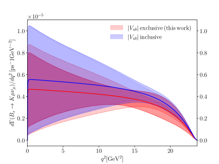
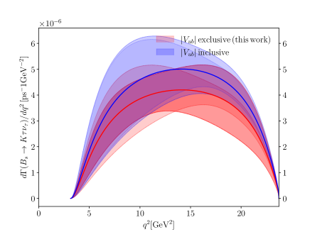
Figure 9: The differential decay width $d\Gamma/dq^{2}$ for $B_{s}\to K\mu\bar{\nu}_{\mu}$ (left) and $B_{s}\to K\tau\bar{\nu}_{\tau}$ (right). The values for $|V_{ub}|$ are taken from Eqs. (50) and (52). The darker (lighter) shading indicates the error without (with) the contribution from the error on $|V_{ub}|$.

V.3.3 $R$ ratios

A second, very important application is to test lepton flavor universality (LFU). LFU is an accidental symmetry in the SM and it is extremely important to test if it holds. One test is to compare these semileptonic decays with electron ($e$), muon ($\mu$) or tau ($\tau$) leptons in the final state. In the SM their couplings with gauge bosons ($W$, $Z$) are identical. However, since their masses differ, the shapes of the partial width distributions with respect to $q^{2}$ will be different and so will be their integrated (or partially integrated) rates. Comparison of measured and predicted rates constitutes another important test of the SM. Particularly interesting and important is to take ratios of integrated rates which are manifestly independent of the mixing angles. Since the mixing angles are known within some uncertainty, LFU tests using the following ratios can be a powerful precision test. Traditionally one introduces,

$$R_{B_{s}\to K}=\frac{\int_{m_{\tau}^{2}}^{q^{2}_{\text{max}}}dq^{2}\,\frac{d\Gamma(B_{s}\to K\tau\bar{\nu}_{\tau})}{dq^{2}}}{\int_{m_{\ell}^{2}}^{q^{2}_{\text{max}}}dq^{2}\,\frac{d\Gamma(B_{s}\to K\ell\bar{\nu}_{\ell})}{dq^{2}}}\,,$$ (53)

and takes the limit of integration from $q^{2}=m_{\ell(\tau)}^{2}$ to the maximum value of $q^{2}$ that is kinematically allowed. In this equation $\ell$ in the denominator stands for $e$ or $\mu$, whereas the numerator is for the tau lepton. Since the electron and muon masses are negligible compared to the mass of the parent $B_{s}$, the contribution to the denominator from the form factor $f_{0}$ is tiny since it is proportional to the lepton mass in the amplitude. This means that for the numerator involving decays to $\tau$, the contribution from the scalar form factor $f_{0}$ cannot be determined experimentally from data for the semileptonic decays into $e$ or $\mu$. The scalar form factor must be calculated from theory in a non-perturbative framework. This realization motivated lattice studies long ago [111].

The conventional definition of $R_{B_{s}\to K}$ in Eq. (53) has a drawback. The contribution to the denominator from $m_{\ell}^{2}\leq q^{2}\leq m_{\tau}^{2}$ has no corresponding contribution in the numerator; thus that region does not give useful information for testing LFU. To emphasize this, imagine $d\Gamma/dq^{2}$ is very peaked for small $q^{2}$. Then the conventional $R_{B_{s}\to K}$, given in (53), would tend to be very small, providing little useful information.

Following Refs. [112, 113], we propose to use another ratio (c.f. Ref. [114]) where we:

• use a common integration range in the numerator and denominator, with lower limit $q^{2}_{\text{min}}\geq m_{\tau}^{2}$ (changing the lower limit was earlier proposed in Refs. [115, 116] as well as in Ref. [113]);

• make the weights multiplying the form factor terms involving $f_{+}(q^{2})$ in the integrands the same for $\tau$ and $\ell$ modes (as in Ref. [113]).

To do this, we rewrite the differential decay rate in Eq. (II.1) in the form

$$\frac{d\Gamma(B_{s}\to K\ell\nu)}{dq^{2}}=\Phi\,\omega_{\ell}(q^{2})\big{[}F_{V}^{2}+(F_{S}^{\ell})^{2}\big{]},$$ (54)

where $\ell$ can be any of $e,\mu,\tau$ and

$$\Phi =\eta_{\text{EW}}\frac{G_{F}^{2}|V_{ub}|^{2}}{24\pi^{3}},$$ (55)

$$\omega_{\ell}(q^{2}) =\bigg{(}1-\frac{m_{\ell}^{2}}{q^{2}}\bigg{)}^{2}\bigg{(}1+\frac{m_{\ell}^{2}}{2q^{2}}\bigg{)},$$ (56)

$$F_{V}^{2} =|{\bf p}_{K}|^{3}|f_{+}(q^{2})|^{2},$$ (57)

$$(F_{S}^{\ell})^{2} =\frac{3}{4}\frac{m_{\ell}^{2}|{\bf p}_{K}|}{m_{\ell}^{2}+2q^{2}}\frac{(M_{B_{s}}^{2}-M_{K}^{2})^{2}}{M_{B_{s}}^{2}}\,|f_{0}(q^{2})|^{2}.$$ (58)

The subscript $\ell$ on $\omega_{\ell}$ and superscript $\ell$ in $(F_{S}^{\ell})^{2}$ show where the dependence on the lepton mass enters. The improved $R$ ratio is now defined by:

$$R^{\text{imp}}_{B_{s}\to K}=\frac{\int_{q^{2}_{\text{min}}}^{q^{2}_{\text{max}}}dq^{2}\,\frac{d\Gamma(B_{s}\to K\tau\bar{\nu}_{\tau})}{dq^{2}}}{\int_{q^{2}_{\text{min}}}^{q^{2}_{\text{max}}}dq^{2}\,\left[\frac{\omega_{\tau}(q^{2})}{\omega_{\ell}(q^{2})}\right]\,\frac{d\Gamma(B_{s}\to K\ell\nu)}{dq^{2}}},$$ (59)

where $\ell$ in the denominator is once again $e$ or $\mu$. With instead a vector meson in the final state, this matches the definition in Ref. [113]. The ratio can be evaluated using experimentally measured differential decay rates. We propose using this ratio as a way to monitor LFU.

We can evaluate the ratio $R^{\text{imp}}_{B_{s}\to K}$ from the Standard Model using our lattice determinations of the form factors. In the approximation that we drop the scalar form factor contribution in the denominator [in (58), $m_{e,\mu}^{2}/2q^{2}\leq m_{\mu}^{2}/2q^{2}\leq m_{\mu}^{2}/2m_{\tau}^{2}=0.002$ in the integration range], we have

$$R^{\text{imp,SM}}_{B_{s}\to K}\approx 1+\frac{\int_{q^{2}_{\text{min}}}^{q^{2}_{\text{max}}}dq^{2}\,\omega_{\tau}(q^{2})(F_{S}^{\tau})^{2}}{\int_{q^{2}_{\text{min}}}^{q^{2}_{\text{max}}}dq^{2}\,\omega_{\tau}(q^{2})F_{V}^{2}}\,,$$ (60)

where now both numerator and denominator have the same weight.

Results for both $R_{B_{s}\to K}$ and $R_{B_{s}\to K}^{\rm impr.}$ are listed in Tab. 11, where we also include our result for the integrated decay rate $\Gamma/|V_{ub}|$. As above, only the results for $K_{+,0}\geq 3$ should be considered to be free of truncation errors in the $z$ expansion. The error we achieve on the new ratio is about three times smaller than for the old ratio. Here is a summary of our central results (based on $(K_{+},K_{0})=(5,5)$):

$$R_{B_{s}\to K}= \,{0.77(16)}\,,$$ (61)

$$R_{B_{s}\to K}^{\rm impr}= \,{1.72(11)}\,.$$ (62)

V.3.4 Forward-backward and polarization asymmetries

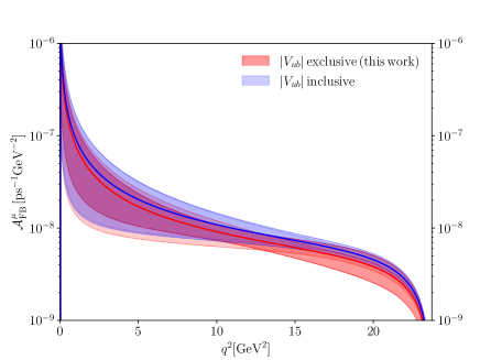
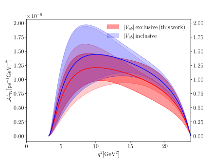
Figure 10: Forward-backward asymmetries $\mathcal{A}_{\rm FB}^{\mu}$ (left) and $\mathcal{A}_{\rm FB}^{\tau}$ (right). For convenient visualization the left-hand plot is shown on a logarithmic scale. The values for $|V_{ub}|$ are taken from Eqs. (50) and (52). The darker (lighter) shading indicates the error without (with) the contribution from the error on $|V_{ub}|$.

Our data for the form factors also allows to compute the forward-backward asymmetry. Starting from the differential decay rate in terms of the lepton angle $\theta_{\ell}$ between the charged-lepton and $B_{s}$ momentum in the $q^{2}$ rest frame. The forward-backward difference is given by

$$\mathcal{A}^{\ell}_{\rm FB}(q^{2})\equiv\left[\int\limits_{0}^{1}-\int\limits_{-1}^{0}\right]d\cos\theta_{\ell}\frac{d^{2}\Gamma(B_{s}\to K\ell\nu)}{dq^{2}d\cos\theta_{\ell}}\,,$$ (63)

and in the SM it takes the form [117]

$$\mathcal{A}^{\ell}_{\rm FB}(q^{2})= \eta_{\text{EW}}\frac{G_{F}^{2}|V_{ub}|^{2}}{32\pi^{3}M_{B_{s}}}\left(1-\frac{m_{\ell}^{2}}{q^{2}}\right)^{2}|{\bf p}_{K}|^{2}$$

$$\times\frac{m_{\ell}^{2}}{q^{2}}\left(M_{B_{s}}^{2}-M_{K}^{2}\right)f_{+}(q^{2})f_{0}(q^{2})\,.$$ (64)

A probe for helicity-violating interactions is provided by the difference of the left-handed and right-handed contributions to the decay rate [117]

$$\mathcal{A}^{\ell}_{\rm pol}(q^{2})=\frac{d\Gamma(\ell,{\rm LH})}{dq^{2}}-\frac{d\Gamma(\ell,{\rm RH})}{dq^{2}}\,,$$ (65)

where

$$\frac{d\Gamma(\ell,{\rm LH})}{dq^{2}}= \eta_{\text{EW}}\frac{G_{F}^{2}|V_{ub}|^{2}|{\bf p}_{K}|^{3}}{24\pi^{3}}\left(1-\frac{m_{\ell}^{2}}{q^{2}}\right)^{2}f_{+}^{2}(q^{2})\,,$$

$$\frac{d\Gamma(\ell,{\rm RH})}{dq^{2}}= \eta_{\text{EW}}\frac{G_{F}^{2}|V_{ub}|^{2}|{\bf p}_{K}|}{24\pi^{3}}\frac{m_{\ell}^{2}}{q^{2}}\left(1-\frac{m_{\ell}^{2}}{q^{2}}\right)^{2}$$

$$\times \left(\frac{3}{8}\frac{(M_{B_{s}}^{2}-M_{K}^{2})^{2}}{M_{B_{s}}^{2}}f_{0}^{2}(q^{2})+\frac{1}{2}|{\bf p}_{K}|^{2}f^{2}_{+}(q^{2})\right)\,.$$

We show our results for the forward-backward asymmetries and the polarization distribution in Figs. 10 and 11, respectively, where the case $\ell=\mu$ ($\tau$) is shown in the left (right) panel. In Tab. 12, we provide numerical results for

$$I[\mathcal{A}^{\ell}]=\int\limits_{m_{\ell}^{2}}^{q^{2}_{\rm max}}dq^{2}\mathcal{A}^{\ell}(q^{2})/|V_{ub}|^{2}\,,$$ (67)

and

$$\mathcal{\bar{A}}^{\ell}=\frac{\int_{m_{\ell}^{2}}^{q_{\rm max}^{2}}dq^{2}\mathcal{A}^{\ell}(q^{2})}{\int_{m_{\ell}^{2}}^{q_{\rm max}^{2}}dq^{2}d\Gamma(B_{s}\to K\ell\nu)/dq^{2}}\,,$$ (68)

where $\mathcal{A}^{\ell}=\mathcal{A}^{\ell}_{\rm FB},\mathcal{A}^{\ell}_{\rm pol}$.

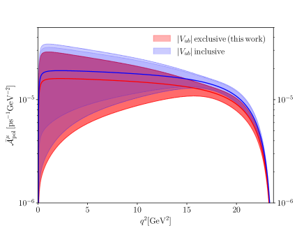
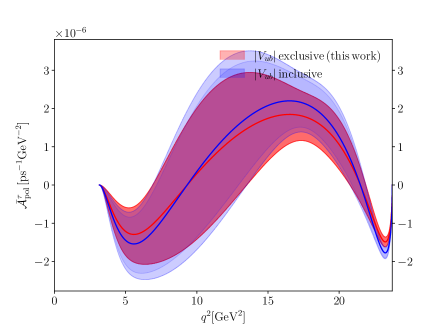
Figure 11: Difference of the left-handed and right-handed contributions to the decay rate $\mathcal{A}_{\rm pol}^{\mu}$ (left) and $\mathcal{A}_{\rm pol}^{\tau}$ (right). The values for $|V_{ub}|$ are taken from Eqs. (50) and (52). The darker (lighter) shading indicates the error without (with) the contribution from the error on $|V_{ub}|$.

Here is a summary of our central results ($(K_{+},K_{0})=(5,5)$)

$$I[\mathcal{A}_{\rm FB}^{\tau}]= \,{1.30(28)}\,{\rm ps}^{-1}\,,$$ (69)

$$I[\mathcal{A}_{\rm FB}^{\mu}]= \,0.040(24)\,{\rm ps}^{-1}\,,$$ (70)

$$\mathcal{\bar{A}}_{\rm FB}^{\tau}= \,0.2821(89)\,,$$ (71)

$$\mathcal{\bar{A}}_{\rm FB}^{\mu}= \,0.0057(18)\,,$$ (72)

$$I[\mathcal{A}_{\rm pol}^{\tau}]= \,0.18(29)\,{\rm ps}^{-1}\,,$$ (73)

$$I[\mathcal{A}_{\rm pol}^{\mu}]= \,6.3(2.3)\,{\rm ps}^{-1}\,,$$ (74)

$$\mathcal{\bar{A}}_{\rm pol}^{\tau}= \,0.035(60)\,,$$ (75)

$$\mathcal{\bar{A}}_{\rm pol}^{\mu}= \,0.9834(49)\,,$$ (76)

and in Fig. 12 we provide a comparison with results from other lattice simulations. Two observations are worth highlighting: With respect to RBC/UKQCD 15 some of the results shifted significantly, and the error of some results increased visibly. The shift is mainly down to our decision to do the HM$\chi$PT chiral and continuum limit for $f_{+}$ and $f_{0}$ rather than for $f_{\perp}$ and $f_{\|}$. The assumption that the same pole masses simultaneously describes the momentum dependence of $f_{+}$ and $f_{\perp}$, and $f_{0}$ and $f_{\|}$, respectively, does not seem correct at the level of precision we achieve with our dataset. The increase in error on the other hand is due to the change in strategy for the BGL parameterization – at the cost of achieving a truncation-independent parameterization of the form factor, the statistical error on observables particularly sensitive to the low-$q^{2}$ behavior of the form factor increases.

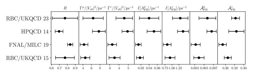
Figure 12: Comparison with results from other collaborations (HPQCD 14 [8], RBC/UKQCD 15 [10], FNAL/MILC 19 [11] and this work, RBC/UKQCD 23).

VI Conclusions

In this paper we present our new results for the non-perturbative Standard Model contributions to the exclusive semileptonic decay $B_{s}\to K\ell\nu$. In particular, we present the results for the form factors $f_{+}(q^{2})$ and $f_{0}(q^{2})$ in the continuum limit of $N_{f}=2+1$ lattice simulations. We have improved our analysis in various ways: a) we have improved the control of the continuum limit by including simulations on a finer ($a^{-1}\approx 2.8\,\text{GeV}$) ensemble. b) we include the effects of excited states in our correlation function fits. c) doing the chiral-continuum extrapolation of $f_{+}$ and $f_{0}$ rather than $f_{\|}$ and $f_{\perp}$ using HM$\chi$PT removes an otherwise irreducible systematic effect present in earlier work [10, 11], which might be the origin of tensions in the combined analysis of lattice results [15]. d) using the Bayesian-inference approach proposed in Ref. [95] to fitting the $z$-parameterization we obtain a model- and truncation-independent parameterization of the form factor in the entire physical semileptonic kinematical range.

Regarding point c) we summarize the situation of available lattice data for the $B_{s}\to K\ell\nu$ form factors in Fig. 13. While all available data for the vector form factor $f_{+}$ is in agreement, the data for $f_{0}$ shows two clusters of data points forming as $q^{2}$ is reduced. The two clusters can be distinguished by the way in which the chiral and continuum limit have been taken. In our view, taking the continuum limit in terms of $f_{+}$ and $f_{0}$ rather than in in terms of $f_{\perp}$ and $f_{\|}$, is correct. The same note of caution concerns other quantities like e.g. $B\to\pi\ell\nu$, where very similar analysis techniques are being used.

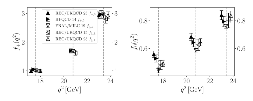
Figure 13: Summary of available lattice data for the $B_{s}\to K\ell\nu$ form factors $f_{+}$ (left) and $f_{0}$ (right) at the same arbitrarily chosen reference points indicated by dashed vertical lines (to improve the presentation, individual data points are shifted slightly in $q^{2}$). Empty symbols indicate the results where the chiral and continuum extrapolations have been carried out in terms of $f_{\perp}$ and $f_{\|}$ and then converted to $f_{+}$ and $f_{0}$ using Eqs. (5) and (II.1), respectively. The points for RBC/UKQCD 23 $f_{\parallel,\perp}$ were generated solely for the purpose of illustration, using the data and analysis methods discussed in this paper, but with the chiral and continuum extrapolation done for $f_{\|}$ and $f_{\perp}$. Filled symbols indicate the results where the extrapolation has been done in terms of $f_{+}$ (left) and $f_{0}$ (right).

We use our results to make a number of predictions for phenomenology. In particular, we make a new prediction for the CKM matrix element $|V_{ub}|=3.78(61)\times 10^{-3}$ based on first results for the $B_{s}\to K\ell\nu$ decay from the LHCb experiment [16]. The error is dominated by the experimental uncertainty. In particular, if we repeat the analysis with the experimental uncertainty set to zero, the error on $|V_{ub}|$ reduces to 0.37. Our result is compatible with both exclusive and inclusive determinations. We also make predictions for the shape of the differential decay rate, the forward-backward asymmetry and the difference between left-handed and right-handed contributions to the decay rate. With more precise experimental and lattice results these observables might in the future allow to shed light on the tension between inclusive and exclusive $|V_{ub}|$ determinations.

Appendix A RHQ parameter tuning

Here we summarize the non-perturbative tuning of the three parameters in the RHQ action used for $b$ quarks. The procedure is described in Ref. [33], based on lattice spacings determined in Ref. [20]. The lattice spacing is a crucial input and with updated and refined global fits available [21, 22, 25], plus new ensembles, we have performed a new tuning for the ensembles used here. More precise determinations of the lattice spacings lead to reduced systematic errors in the RHQ parameters. In addition, the values for the strange-quark mass have been reanalyzed and we have generated new valence-quark propagators with mass tuned or close to the updated strange-quark mass.

A.1 Non-perturbative tuning procedure

The parameters in the RHQ action, $\{m_{0}a,c_{P},\zeta\}$, are fixed by demanding that the action correctly describes experimentally measured on-shell $B_{s}$-meson properties. We match the experimental values [75] of the spin-averaged mass and the hyperfine splitting, and require that the rest and kinetic masses of the $B_{s}$ are equal

$$\overline{M}_{\!B_{s}}=\frac{M_{\!B_{s}}\!+\!3M_{\!B^{*}_{s}}}{4},\quad\Delta M_{\!B_{s}}=M_{\!B^{*}_{s}}-M_{\!B_{s}},\quad\frac{M_{1}^{B_{s}}}{M_{s}^{B_{s}}}=1.$$ (77)

The latter implies that the $B_{s}$ meson satisfies the continuum dispersion relation, $E^{2}_{B_{s}}({\bf p})={\bf p}\,^{2}+M^{2}_{B_{s}}$. We calculate the quantities above using seven sets of choices for the RHQ parameters $\{m_{0}a$, $c_{P}$, $\zeta\}$ and then make a linear interpolation to find the values satisfying the matching conditions above. The seven choices, indexed 1 to 7 from left to right, comprise a central set plus variations of each of the three parameters:

$$\begin{bmatrix}m_{0}a\\ c_{P}\\ \zeta\end{bmatrix}\!\!, \begin{bmatrix}m_{0}a-\sigma_{m_{0}a}\\ c_{P}\\ \zeta\end{bmatrix}\!\!,\begin{bmatrix}m_{0}a+\sigma_{m_{0}a}\\ c_{P}\\ \zeta\end{bmatrix}\!\!,\begin{bmatrix}m_{0}a\\ c_{P}-\sigma_{c_{P}}\\ \zeta\end{bmatrix}\!\!,$$

$$\begin{bmatrix}m_{0}a\\ c_{P}+\sigma_{c_{P}}\\ \zeta\end{bmatrix}\!\!,\begin{bmatrix}m_{0}a\\ c_{P}\\ \zeta-\sigma_{\zeta}\end{bmatrix}\!\!,\begin{bmatrix}m_{0}a\\ c_{P}\\ \zeta+\sigma_{\zeta}\end{bmatrix}\!\!.$$ (78)

We make a constant-plus-linear ansatz for the dependence of the observables on the RHQ parameters

$$\begin{bmatrix}\overline{M}_{B_{s}}\\ \Delta M_{B_{s}}\\ M_{1}^{B_{s}}/M_{2}^{B_{s}}\end{bmatrix}=J\cdot\begin{bmatrix}m_{0}a\\ c_{P}\\ \zeta\end{bmatrix}+A\,.$$ (79)

Here $J$ represents the “slope” and is a $3\times 3$ matrix, while $A$ corresponds to the intercept and is a $3\times 1$ vector. In a region with sufficiently linear dependence on the parameters, we can obtain $J$ and $A$ using finite differences to approximate derivatives:

$$J =\left[\frac{Y_{3}-Y_{2}}{2\sigma_{m_{0}a}},\,\frac{Y_{5}-Y_{4}}{2\sigma_{c_{P}}},\,\frac{Y_{7}-Y_{6}}{2\sigma_{\zeta}}\right],$$ (80)

$$A =Y_{1}-J\cdot\left[m_{0}a,\,c_{P},\,\zeta\right]^{T}.$$

The vectors $Y_{i}$ are constructed from the values of meson masses and splittings measured on the $i^{\textrm{th}}$ parameter set in (A.1),

$$Y_{i}=\left[\overline{M}_{B_{s}},\Delta M_{B_{s}},M_{1}^{B_{s}}/M_{2}^{B_{s}}\right]^{T}_{i}.$$ (81)

Inverting Eq. (79), we obtain the tuned RHQ parameters

$$\begin{bmatrix}m_{0}a\\ c_{P}\\ \zeta\end{bmatrix}^{\text{RHQ}}=J^{-1}\cdot\left(\begin{bmatrix}\overline{M}_{\!B_{s}}\\ \Delta M_{B_{s}}\\ M_{1}^{B_{s}}/M_{2}^{B_{s}}\end{bmatrix}^{\text{PDG}}\!\!-A\right),$$ (82)

by matching to PDG values and demanding the $B_{s}$ rest mass equals its kinetic mass. Specifically we use [75].

$$\overline{M}_{B_{s}} =\frac{1}{4}\big{(}5366.82^{+0.22}_{-0.22}+3\cdot 5415.4^{+1.8}_{-1.4}\big{)}\,\text{MeV}$$ (83)

$$=5403.26^{+1.8}_{-1.4}\,\text{MeV},$$

$$\Delta M_{B_{s}} =48.6^{+1.8}_{-1.6}\,\text{MeV}.$$

We conservatively use the full error on $M_{B_{s}^{*}}$ as the uncertainty of the spin-averaged mass. The relative error on $\Delta_{M_{B_{s}}}$ is much larger and will dominate systematic effects due to the experimental inputs. These inputs are updated from those in Ref. [118] used in Ref. [33].

A.2 Lattice simulations

The tuning procedure is implemented by first determining $B_{s}^{(*)}$-meson energies for zero and non-zero momenta on our set of ensembles in Table 1. We calculate two-point functions by contracting strange-quark propagators using point source and point sink with Gaussian source-smeared, point-sink $b$-quark propagators, and extract $B_{s}^{(*)}$-meson energies from correlated fits to the plateau of effective energies. We find good correlated confidence levels ($p$-value $\gtrsim$ 10%) in all cases and varying the fitting range by $\pm 1$ time slice changes the result only within the statistical uncertainty. The value of our input strange-quark mass as well as the width $\sigma_{G}$ and the number of iterations $N_{G}$ for the Gaussian source smearing of the $b$ quarks are summarized in Table 13 together with the fitting range used to extract the $B_{s}^{(s)}$ meson energies.

Table 13: Input strange quark mass $am_{s}$, width $\sigma_{G}$ and iteration count $N_{G}$ of the Gaussian source smearing used to calculate $B_{s}^{(*)}$ meson two-point functions. We extract the $B_{s}^{(*)}$ energies by performing correlated fits using the specified fit ranges. The optimal Gaussian source-smearing radius was explored for the C and M ensembles in Ref. [33] and we scaled those results to the finer lattice spacing $a^{-1}=2.785\,\text{GeV}$ on the F1S ensemble.

	$a^{-1}/\!\,\text{GeV}$	$L^{3}$	$a(m_{s}+m_{\text{res}}$)	$\sigma_{G}$	$N_{G}$	fit range
C	1.785	$24^{3}$	0.03224+0.00315	17.86	100	[10:25]
M	2.383	$32^{3}$	0.025+0.00067	10.36	170	[12:21]
F	2.785	$48^{3}$	0.02144+0.00094	12.14	230	[14:29]

Starting from the tuning performed in Ref. [33], we iterate twice to find the new central set of RHQ parameters for the C and M ensembles and choose roughly three times the size of the statistical errors for the variations $\sigma_{\{m_{0}a,c_{P},\zeta\}}$. For the new F1S ensemble at the finer lattice spacing, we roughly scaled our new results on C and M ensembles and then carried out two iterations choosing variations $\sigma_{\{m_{0}a,c_{P},\zeta\}}$ of roughly 1.5 times the statistical uncertainties. In all cases our final parameter sets allow us to interpolate to the values of $m_{0}a$, $c_{P}$, and $\zeta$ describing physical $b$ quarks and we do not observe any signs of curvature within the explored parameter ranges. The final values of the central parameter sets and their variations are listed in Table 14.

Table 14: Central parameter set $\{m_{0}a,\,c_{P},\,\zeta\}$ with variations $\sigma_{m_{0}a},\,\sigma_{c_{P}},\,\sigma_{\zeta}$ for the final iteration of tuning the parameters on C, M and F ensembles with inverse lattice spacings ranging from $1.785$ to $2.785\,\text{GeV}$.

	$a^{-1}\!/\!\,\text{GeV}$	$L^{3}$	$m_{0}a\pm\sigma_{m_{0}a}$	$c_{P}\pm\sigma_{c_{P}}$	$\zeta\pm\sigma_{\zeta}$
C	1.785	$24^{3}$	7.42 $\pm$ 0.18	4.86 $\pm$ 0.42	2.92 $\pm$ 0.21
M	2.383	$32^{3}$	3.46 $\pm$ 0.09	3.03 $\pm$ 0.24	1.75 $\pm$ 0.10
F	2.785	$48^{3}$	2.35 $\pm$ 0.20	2.75 $\pm$ 0.30	1.50 $\pm$ 0.15

Using those values, we determine spin-averaged masses, hyperfine splittings and ratios of rest mass over kinetic mass in order to match to experimental results reported by the PDG as in Eq. (83). We finally obtain our tuned parameters from Eq. (82). For the C and M ensembles we cannot resolve a dependence on the light sea-quark mass within statistical errors. Hence, we average the values at the same lattice spacing. We report these results, plus the outcome for tuning on the F1S ensemble, in Table 15.

Table 15: Tuned RHQ parameter values for all lattices determined using the parameter sets specified in Tab. 14. For the C and M lattices, we see no dependence on the light sea-quark mass within statistical errors and we consequently compute weighted averages to obtain our preferred values.

$am_{l}$	$m_{0}a$	$c_{P}$	$\zeta$
C: $a^{-1}=1.785\,\text{GeV}$, $24^{3}\times 64$
0.005	7.468(66)	4.87(18)	2.922(82)
0.010	7.476(80)	4.97(19)	2.94(10)
average	7.471(51)	4.92(13)	2.929(63)
M: $a^{-1}=2.383\,\text{GeV}$, $32^{3}\times 64$
0.004	3.541(46)	3.19(13)0	1.715(55)
0.006	3.474(37)	3.01(10)0	1.759(46)
0.008	3.444(48)	3.02(14)0	1.807(55)
average	3.485(25)	3.063(69)	1.760(30)
F: $a^{-1}=2.785\,\text{GeV}$, $48^{3}\times 96$
0.002144	2.423(62)	2.68(13)	1.523(79)

A.3 Estimating systematic uncertainties

Table 16: Systematic uncertainties in percent with a significant effect on our tuned RHQ parameters. For the C and M ensembles we always report the largest fluctuation observed on either ensemble.

uncertainty	$a^{-1}\!/\!\,\text{GeV}$	$m_{0}a$	$c_{P}$	$\zeta$
heavy quark discretization	1.785	1.0%	5.6%	3.4%
	2.383	1.1%	6.0%	3.3%
	2.785	1.5%	5.6%	2.8%
lattice scale	1.785	1.1%	1.4%	0.5%
	2.383	1.3%	1.7%	0.4%
	2.785	1.3%	1.4%	0.3%
experiment	1.785	0.6%	4.8%	0.1%
	2.383	0.9%	5.0%	0.1%
	2.785	1.2%	4.8%	0.1%

A.3.1 Heavy-quark-discretization errors

When $m_{0}a\sim 1$, the RHQ action leads to a nontrivial lattice-spacing dependence of physical quantities. As discussed in detail in Ref. [33], we estimate the discretization errors for the heavy sector using power counting, following Oktay and Kronfeld [119]. Since we are considering the same physical quantities, spin-averaged mass, hyperfine splitting, and ratio of rest over kinetic mass, we simply list uncertainties in percent and refer to Appendix C of Ref. [33] for further details.

$$\text{error}^{M_{1,B_{s}}}_{\text{total}} =0.05\%,$$ (84)

$$\text{error}^{M_{2,B_{s}}}_{\text{total}} =2.59\%,$$

$$\text{error}^{\Delta M_{B_{s}}}_{\text{total}} =4.40\%.$$

By assigning these errors as uncertainty in our inputs to the matching procedure, we propagate them to the RHQ parameters and collect the percentage changes in the central values in the first panel of Table 16.

A.3.2 Input strange-quark mass

Our RHQ parameters are tuned using strange quark propagators corresponding to a mass at or near the physical strange-quark mass. We need to account for slight mistunings as well as for the uncertainty in the strange-quark mass quoted in Ref. [21, 22] (see also table 1).

On the coarse (C) ensembles, we can bracket the strange quark mass using the additional quark propagators with bare masses $am_{s}^{\prime}=0.03$ and $0.04$. This allows us to determine numerically the slopes of $m_{0}$, $c_{P}$, and $\zeta$ with respect to the strange quark mass. Since the mass of our strange quark propagators matches the physical value, we read off the changes in $m_{0}a$, $c_{P}$, and $\zeta$ after varying $am_{s}$ by $\pm 1\sigma$. The largest change we observe is $0.2\%$.

For the M ensembles we simulate with a bare strange quark mass of $0.025$ which is roughly $1\sigma$ larger than the physical value. Using in addition $am_{s}^{\prime}=0.0272$, we determine the slopes with respect to $m_{s}$ and estimate the error due to mistuning as well as the uncertainty in the strange quark mass by varying the strange quark mass by $\pm 2\sigma$. Our RHQ parameters change at most by $0.3\%$.

For the F1S ensemble, since the slopes with respect to $am_{s}$ decrease as the lattice spacing decreases, we use for simplicity the average of the slopes obtained on the M ensembles to estimate the uncertainty due to the input strange quark mass for F1S. Here our value for the mass of the strange quark is within $1\sigma$ of the physical value. Being conservative we vary the strange quark mass by $\pm 2\sigma$ and read off changes of the RHQ parameters of at most $0.2\%$.

Given that for all ensembles and all three RHQ parameters the uncertainty due to the strange quark mass is $0.3\%$ or less, we consider this effect negligible compared to the percent-level uncertainties arising from, for example, heavy quark discretization errors.

A.3.3 Lattice scale uncertainty

The lattice scale enters our tuning procedure when we convert the experimental input data to lattice units. To propagate the uncertainty of the lattice spacings to our RHQ parameters, we repeat the analysis varying the lattice spacing by $\pm 1\sigma$. For the C and M ensembles we take the largest fluctuation of a central value on either ensemble as our estimate.

A.3.4 Experimental uncertainty

We estimate the uncertainty due to the experimental inputs by varying both the spin-averaged mass and the hyperfine splitting by $\pm 1\sigma$ each and re-run our matching analysis. In practice, the uncertainty in the spin-averaged mass is negligible compared to the few-percent effect due to the uncertainty in the hyperfine splitting. We take the largest change of the central values at a given lattice spacing as our estimate for the corresponding uncertainty in our RHQ parameters.

A.4 Tuned RHQ parameters

We summarize our tuned RHQ parameters in Table 17 quoting our final results with all systematic errors found to be significant.

Table 17: Values of the tuned RHQ parameters with central values and statistical errors taken from table 15 and estimates for the systematic errors from table 16. Tuning determines the bare quark mass, $m_{0}a$, clover coefficient, $c_{P}$ and anisotropy parameter, $\zeta$, in the RHQ action. Errors listed for $m_{0}a$, $c_{P}$, and $\zeta$ are, from left to right: statistics, heavy-quark discretization errors, the lattice scale uncertainty, and the uncertainty due to the experimental measurement of the $B_{s}$ meson hyperfine splitting, respectively. Other errors considered but found to be negligible are not shown.

	$a^{-1}\!/\!\,\text{GeV}$	$m_{0}a$	$c_{P}$	$\zeta$
C	1.785	7.471(51)(75)(82)(45)	4.92(13)(28)(07)(24)	2.929(63)(100)(15)(03)
M	2.383	3.485(25)(38)(45)(31)	3.06(07)(18)(05)(15)	1.760(30)(58)(07)(02)1
F	2.785	2.423(62)(36)(31)(29)	2.68(13)(15)(04)(13)	1.523(79)(43)(05)(02)1

Appendix B RHQ discretization errors

Table 18: Values of the mismatch functions defined in Appendix B of Ref. [38] for the non-perturbatively tuned parameters of the RHQ action given in Table 17. The tree-level coefficients $f_{E}$, $f_{X_{i}}$, and $f_{Y}$ are known exactly. The two-loop coefficient $f_{3}^{[2]}$ is not known, so we use an ansatz based on the tree-level expression. The coupling $\alpha_{s}(a^{-1})$ needed to evaluate $f_{3}^{[2]}$ is taken to be a lattice mean-field coupling at the (inverse) lattice spacing scale (see the discussion of the perturbative calculations in section II.3).

	$a^{-1}\!/\!\,\text{GeV}$	$\alpha_{s}(a^{-1})$	$f_{E}$	$f_{X_{1}}$	$f_{X_{2}}$	$f_{Y}$	$f_{3}^{[2]}$
C	1.785	0.2320	0.0594	0.0848	0.1436	0.1358	0.0333
M	2.383	0.2155	0.0809	0.0966	0.1691	0.1721	0.0298
F	2.785	0.2083	0.1042	0.1101	0.1946	0.2056	0.0299

Table 19: Percentage errors from mismatches in the action and current for the bottom quark. For this estimate, we calculate the mismatch functions for the non-perturbatively-tuned parameters of the RHQ action from table 17. We estimate the size of operators using HQET power counting with $\Lambda_{\text{QCD}}=500\,\text{MeV}$ and $\alpha_{s}^{\overline{\text{MS}}}(a^{-1})$. To obtain the total, we add the individual errors in quadrature, including each contribution the number of times that operator occurs. Contribution ‘E’ is counted twice, while ‘3’ is counted twice for $f_{\|}$ and four times for $f_{\perp}$. The definitions of operators ‘E’, ‘X₁’, ‘X₂’, ‘Y’ and ‘3’, and expressions for the mismatch functions, are given in Appendix B of Ref. [38].

			$O(a^{2})$ error	$O(a^{2})$ errors			$O(\alpha_{s}^{2}a)$ error
			from action	from current			from current	Total/%
	$a^{-1}\!/\!\,\text{GeV}$	$\alpha_{s}(a^{-1})$	E	X1	X2	Y	3	$f_{\|}$	$f_{\perp}$
C	1.785	0.2320	0.47	0.67	1.13	1.07	0.93	2.24	2.60
M	2.383	0.2155	0.36	0.43	0.74	0.76	0.63	1.53	1.77
F	2.785	0.2083	0.34	0.35	0.63	0.66	0.54	1.33	1.53

We tune the parameters in the RHQ action non-perturbatively, such that the leading heavy-quark discretization errors from the action are $O(a^{2})$. We use an $O(\alpha_{s}a)$-improved vector current and calculate the improvement coefficient to $1$-loop; hence the leading heavy-quark discretization errors from the current are of $O(\alpha_{s}^{2}a,a^{2})$. Table 18 gives values for the ‘mismatch’ functions at each of our lattice spacings, from which we find and list in Table 19 the estimated heavy quark discretization errors from the five different operators in the action and current. We refer the reader to section V.E and appendix B of Ref. [38] for further details.

Appendix C Renormalization and improvement coefficients

Table 2 summarizes the values of the renormalization constants $Z^{ll}_{A}(am_{l})$.

Table 20: Residual renormalization factors and operator improvement coefficients. We compute the $\rho$ factors and the matching coefficients $c_{i}^{n}$ at one loop in mean-field improved lattice perturbation theory [43]. They are evaluated for the tuned RHQ bare-quark mass $m_{0}a$ at each lattice spacing (indicated by the letters C, M and F in column headers, see table 1) and for the choices of the domain-wall height $M_{5}=1.8$ The values are an average from four combinations of mean link and strong coupling, with the columns headed $\Delta$ giving the spread in values from the four combinations.

	C $M_{5}=1.8$		M $M_{5}=1.8$		F $M_{5}=1.8$
	value	$\Delta$	value	$\Delta$	value	$\Delta$
$\rho_{V_{0}}$	$1.0301$	$0.0115$	$1.0177$	$0.0059$	$1.0130$	$0.0041$
$\rho_{V_{i}}$	$0.9959$	$0.0019$	$0.9926$	$0.0022$	$0.9921$	$0.0019$
$c_{t}^{3}$	$0.0599$	$0.0092$	$0.0574$	$0.0073$	$0.0550$	$0.0064$
$c_{t}^{4}$	$-0.0120$	$0.0042$	$-0.0109$	$0.0030$	$-0.0101$	$0.0025$
$c_{s}^{1}$	$-0.0010$	$0.0006$	$-0.0015$	$0.0006$	$-0.0018$	$0.0006$
$c_{s}^{2}$	$0.0020$	$0.0021$	$0.0004$	$0.0011$	$-0.0001$	$0.0009$
$c_{s}^{3}$	$0.0512$	$0.0060$	$0.0497$	$0.0050$	$0.0478$	$0.0044$
$c_{s}^{4}$	$-0.0038$	$0.0020$	$-0.0022$	$0.0011$	$-0.0015$	$0.0008$

In Table 20 we give the residual renormalization factors and the improvement coefficients for the heavy-light currents with a heavy RHQ and a light domain-wall quark, computed at one loop order [43] in mean-field improved perturbation theory.

Table 21: Inputs for numerical evaluation of perturbatively computed coefficients at the three different lattice spacings in our ensembles.

	C	M	F
$a^{-1}/\,\text{GeV}$	1.785	2.383	2.785
$\beta$	2.13	2.25	2.31
$\langle P\rangle$	0.588011	0.615580	0.627970
$\langle R_{1}\rangle$	0.343464	0.379841	0.396626
$u_{P}$	0.875682	0.885770	0.890194
$u_{L}$	0.843997	0.860991	0.868440
$m_{0}a$	7.471	3.485	2.423
$\alpha^{\overline{\text{MS}}}_{s,\text{lat}}(a^{-1})$	0.2320	0.2155	0.2083
$\alpha^{\overline{\text{MS}}}_{s,\text{ctm}}(a^{-1})$	0.3226	0.2811	0.2633

Table 21 gives inputs used for numerical evaluation of the perturbatively calculated coefficients. Mean-field improvement uses values for the average gauge link, $u$. We use either the fourth root of the plaquette expectation value, denoted $u_{P}$, or the mean link in Landau gauge, $u_{L}$. We use two choices of strong coupling: a mean-field lattice $\overline{\text{MS}}$ strong coupling, $\alpha^{\overline{\text{MS}}}_{s,\text{lat}}$, or the continuum $\overline{\text{MS}}$ strong coupling, $\alpha^{\overline{\text{MS}}}_{s,\text{ctm}}$, both evaluated at the scale $\mu=a^{-1}$. For the Iwasaki gauge action used for our gauge field ensembles, the lattice strong coupling depends on the plaquette and rectangle expectation values $\left<P\right>$ and $\left<R_{1}\right>$ respectively, quoted in Table 21. For the continuum coupling, we use 5-loop running from RunDec [120, 121, 122], starting from $\alpha^{(5)}(\bar{m}_{b}(\bar{m}_{b}))=0.2268$ at $\bar{m}_{b}(\bar{m}_{b})=4.163\,\text{GeV}$ (The same choice was made when using RunDec to compute $\bar{m}_{b}(2\,\text{GeV})$ for evaluating the $\chi$ factors in the outer functions for BGL $z$-fits. See appendix D). The perturbative results in Table 21 are the average of values from the four combinations of $u$ and $\alpha^{\overline{\text{MS}}}_{s}$. The columns headed $\Delta$ give half of the spread in the values from the four combinations.

Appendix D BGL fits

Here we give expressions for the Blaschke factors and outer functions used in BGL fits to form factors.

The Blaschke factor $B_{X}(q^{2})$ is chosen to vanish at the positions of sub-threshold poles sitting between $q^{2}_{\text{max}}$ and $t_{*}$, with $t_{*}$ denoting the squared momentum transfer for the lowest two-particle production threshold. If there are $n$ such poles with masses $m_{i}$ and corresponding $z$-values $z_{i}=z(m_{i}^{2};t_{*},t_{0})$, then

$$B_{X}(q^{2})=\prod_{i=0}^{n-1}\frac{z-z_{i}}{1-\bar{z}_{i}z}=\prod_{i=0}^{n-1}z(q^{2};t_{*},m_{i}^{2}),$$ (85)

where $z=z(q^{2};t_{*},t_{0})$ and $\bar{z}_{i}$ is the complex conjugate of $z_{i}$ in the first form of the expression. The function $z(q^{2};t_{*},t_{0})$ is defined in Eq. (32) and our choice for $t_{0}$ is given in Eq. (33). For $B_{s}\to K\ell\nu$ decays the threshold is $M_{B}+M_{\pi}=5.4175\,\text{GeV}$ and there is a sub-threshold pole at $M_{B^{*}}=5.32471\,\text{GeV}$ [50] for $f_{+}$, but not for $f_{0}$ for which $M_{B^{*}(0^{+})}=5.63\,\text{GeV}$ [51] is above threshold.

The outer functions used in the parameterizations of $f_{+}$ and $f_{0}$ take the form [84, 89, 91]

$$\phi_{+}(q^{2},t_{0}) =\sqrt{\frac{\eta_{I}}{48\pi\chi_{1^{-}}(0)}}\,\frac{r_{q}^{1/2}}{r_{0}^{1/2}}\,(r_{q}+r_{0})\big{(}r_{q}+\sqrt{t_{*}}\,\big{)}^{-5}$$

$$\qquad\times(t_{+}-q^{2})^{3/4}(r_{q}+r_{-})^{3/2}\,,$$ (86)

$$\phi_{0}(q^{2},t_{0}) =\sqrt{\frac{\eta_{I}t_{+}t_{-}}{16\pi\chi_{0^{+}}(0)}}\,\frac{r_{q}^{1/2}}{r_{0}^{1/2}}\,(r_{q}+r_{0})\big{(}r_{q}+\sqrt{t_{*}}\,\big{)}^{-4}$$

$$\qquad\times(t_{+}-q^{2})^{1/4}(r_{q}+r_{-})^{1/2}\,,$$ (87)

where we have set $r_{q}=\sqrt{t_{*}-q^{2}}$, $r_{-}=\sqrt{t_{*}-t_{-}}$ and $r_{0}=\sqrt{t_{*}-t_{0}}$ ($t_{\pm}$ are defined after Eq. (32)). The $\chi_{J}(0)$ come from evaluating the vacuum polarization function of two currents ($\bar{b}\gamma_{\mu}u$ and its Hermitian conjugate), while the $\eta_{I}$ are isospin factors counting accessible isospin-related states when inserting a sum over states between the two currents in the vacuum polarization function (to derive the unitarity constraint on the form factors). For $B_{s}\to K\ell\nu$ we have $\eta_{I}=1$.

The $\chi_{J}(0)$ have condensate contributions and perturbative parts. Expressions with the perturbative parts to two loops are given in Ref. [124] and three-loop perturbative contributions have been calculated by Grigo et al. in Ref. [125] (the expressions in Ref. [124] use pole masses while those in Ref. [125] use $\overline{\text{MS}}$ masses; we checked that they agree once the scheme conversion needed to relate them is used). For $B_{s}\to K\ell\nu$ decays, with $x=u$, $\chi_{J}(0)$ is evaluated using $u=m_{x}/m_{b}=0$.

We evaluate the perturbative contributions using the results from Ref. [125] and following the procedure used in Ref. [123], with input $\overline{\text{MS}}$ masses $\bar{m}_{b}(\bar{m}_{b})=4.163(16)\,\text{GeV}$ and $\bar{m}_{c}(3\,\text{GeV})=0.986(13)\,\text{GeV}$ from Ref. [126], and $\alpha_{s}^{(5)}\big{(}\bar{m}_{b}(\bar{m}_{b})\big{)}=0.2268(23)$). To evaluate the condensate contribution for $B_{s}\to K\ell\nu$, we ran the $b$ mass to $\bar{m}_{b}(2\,\text{GeV})=4.95\,\text{GeV}$ using the RunDec package [120, 121, 122] and combined it with $\langle\bar{u}u\rangle_{\mu=2\,\text{GeV}}=-(274\,\text{MeV})^{3}$, from a weighted mean of $2+1+1$ and $2+1$ flavor estimates for $\Sigma^{1/3}$ in SU(2) in the 2021 FLAG review [15, 127, 128, 129, 130, 131, 132, 133, 134]), giving $\bar{m}_{b}\langle\bar{u}u\rangle=-0.102\,\text{GeV}^{4}$. We took $\langle\alpha_{s}G^{2}\rangle=0.0635(35)\,\text{GeV}^{4}$ from a sum rules average [135]. We find

$$\chi_{1^{-}}(0) =6.03\times 10^{-4}\,\text{GeV}^{-2}$$ (88)

$$\chi_{0^{+}}(0) =1.48\times 10^{-2}\,.$$

The values of $\chi_{J}(0)$ and $\eta_{I}$ are needed for checking or imposing the unitarity constraint on each form factor. If the constraint is not saturated then their values do not affect the physical result of a $z$-fit since they are a normalization which can be absorbed by an overall factor in the fit coefficients.

In Ref. [103] the two susceptibilities were computed non-perturbatively,

$$\chi_{1^{-}}(0) =4.45(1.16)\times 10^{-4}\,{\rm GeV}^{-2}\,,$$ (89)

$$\chi_{0^{+}}(0) =2.04(0.20)\times 10^{-2}\,.$$

We do not observe any significant changes in our results for observables when using these values instead of those in Eq. (88).

References

- Aaij et al. [2013] R. Aaij et al. (LHCb), Measurement of Form-Factor-Independent Observables in the Decay , Phys. Rev. Lett. 111, 191801 (2013), arXiv:1308.1707 [hep-ex] .
- Aaij et al. [2014] R. Aaij et al. (LHCb), Test of lepton universality using decays, Phys. Rev. Lett. 113, 151601 (2014), arXiv:1406.6482 [hep-ex] .
- Lees et al. [2012a] J. P. Lees et al. (BaBar), Evidence for an excess of decays, Phys. Rev. Lett. 109, 101802 (2012a), arXiv:1205.5442 [hep-ex] .
- Lees et al. [2013] J. P. Lees et al. (BaBar), Measurement of an Excess of Decays and Implications for Charged Higgs Bosons, Phys. Rev. D 88, 072012 (2013), arXiv:1303.0571 [hep-ex] .
- Huschle et al. [2015] M. Huschle et al. (Belle), Measurement of the branching ratio of relative to decays with hadronic tagging at Belle, Phys. Rev. D 92, 072014 (2015), arXiv:1507.03233 [hep-ex] .
- Aaij et al. [2015] R. Aaij et al. (LHCb), Measurement of the ratio of branching fractions , Phys. Rev. Lett. 115, 111803 (2015), [Erratum: Phys.Rev.Lett. 115, 159901 (2015)], arXiv:1506.08614 [hep-ex] .
- LHC [2022] Measurement of lepton universality parameters in and decays, (2022), arXiv:2212.09153 [hep-ex] .
- Bouchard et al. [2014] C. Bouchard, G. P. Lepage, C. Monahan, H. Na, and J. Shigemitsu, form factors from lattice QCD, Phys.Rev. D90, 054506 (2014), arXiv:1406.2279 [hep-lat] .
- Monahan et al. [2018] C. J. Monahan, C. M. Bouchard, G. P. Lepage, H. Na, and J. Shigemitsu, Form factor ratios for and semileptonic decays and , Phys. Rev. D98, 114509 (2018), arXiv:1808.09285 [hep-lat] .
- Flynn et al. [2015] J. M. Flynn, T. Izubuchi, T. Kawanai, C. Lehner, A. Soni, R. S. Van de Water, and O. Witzel (RBC/UKQCD), and form factors and from -flavor lattice QCD with domain-wall light quarks and relativistic heavy quarks, Phys. Rev. D91, 074510 (2015), arXiv:1501.05373 [hep-lat] .
- Bazavov et al. [2019] A. Bazavov et al. (Fermilab/MILC), decay from lattice QCD, Phys. Rev. D100, 034501 (2019), arXiv:1901.02561 [hep-lat] .
- Bahr et al. [2016] F. Bahr, D. Banerjee, F. Bernardoni, A. Joseph, M. Koren, H. Simma, and R. Sommer (ALPHA), Continuum limit of the leading-order HQET form factor in decays, Phys. Lett. B757, 473 (2016), arXiv:1601.04277 [hep-lat] .
- Witzel [2020] O. Witzel, Lattice QCD (focus on Charm and Beauty form factors, , - & -quark masses), 18th International Conference on B-Physics at Frontier Machines, PoS Beauty2019, 037 (2020), arXiv:2002.01056 [hep-ph] .
- Lytle [2020] A. Lytle, Lattice form factors, , and , PoS LATTICE2019, 228 (2020), arXiv:2004.01132 [hep-lat] .
- Aoki et al. [2022] Y. Aoki et al. (Flavour Lattice Averaging Group (FLAG)), FLAG Review 2021, Eur. Phys. J. C 82, 869 (2022), arXiv:2111.09849 [hep-lat] .
- Aaij et al. [2021] R. Aaij et al. (LHCb), First observation of the decay and measurement of , Phys. Rev. Lett. 126, 081804 (2021), arXiv:2012.05143 [hep-ex] .
- Na et al. [2015] H. Na, C. M. Bouchard, G. P. Lepage, C. Monahan, and J. Shigemitsu (HPQCD), form factors at nonzero recoil and extraction of , Phys. Rev. D92, 054510 (2015), arXiv:1505.03925 [hep-lat] .
- Sirlin [1982] A. Sirlin, Large , behavior of the corrections to semileptonic processes mediated by , Nucl. Phys. B196, 83 (1982).
- Allton et al. [2008] C. Allton et al. (RBC/UKQCD), Physical Results from 2+1 Flavor Domain Wall QCD and SU(2) Chiral Perturbation Theory, Phys. Rev. D78, 114509 (2008), arXiv:0804.0473 [hep-lat] .
- Aoki et al. [2011] Y. Aoki et al. (RBC/UKQCD), Continuum Limit Physics from 2+1 Flavor Domain Wall QCD, Phys.Rev. D83, 074508 (2011), arXiv:1011.0892 [hep-lat] .
- Blum et al. [2016] T. Blum et al. (RBC/UKQCD), Domain wall QCD with physical quark masses, Phys. Rev. D93, 074505 (2016), arXiv:1411.7017 [hep-lat] .
- Boyle et al. [2017] P. A. Boyle, L. Del Debbio, A. Jüttner, A. Khamseh, F. Sanfilippo, and J. T. Tsang (RBC/UKQCD), The decay constants and in the continuum limit of domain wall lattice QCD, JHEP 12, 008, arXiv:1701.02644 [hep-lat] .
- Shamir [1993] Y. Shamir, Chiral fermions from lattice boundaries, Nucl. Phys. B406, 90 (1993), arXiv:hep-lat/9303005 .
- Furman and Shamir [1995] V. Furman and Y. Shamir, Axial symmetries in lattice QCD with Kaplan fermions, Nucl. Phys. B439, 54 (1995), arXiv:hep-lat/9405004 .
- Boyle et al. [2018] P. A. Boyle, L. Del Debbio, N. Garron, A. Jüttner, A. Soni, J. T. Tsang, and O. Witzel (RBC/UKQCD), SU(3)-breaking ratios for and mesons, (2018), arXiv:1812.08791 [hep-lat] .
- Kaplan [1992] D. B. Kaplan, A Method for simulating chiral fermions on the lattice, Phys. Lett. B288, 342 (1992), arXiv:hep-lat/9206013 .
- Blum and Soni [1997a] T. Blum and A. Soni, QCD with domain wall quarks, Phys. Rev. D56, 174 (1997a), arXiv:hep-lat/9611030 [hep-lat] .
- Blum and Soni [1997b] T. Blum and A. Soni, Domain wall quarks and kaon weak matrix elements, Phys. Rev. Lett. 79, 3595 (1997b), arXiv:hep-lat/9706023 [hep-lat] .
- Brower et al. [2017] R. C. Brower, H. Neff, and K. Orginos, The Möbius domain wall fermion algorithm, Comput. Phys. Commun. 220, 1 (2017), arXiv:1206.5214 [hep-lat] .
- Christ et al. [2007] N. H. Christ, M. Li, and H.-W. Lin, Relativistic heavy quark effective action, Phys.Rev. D76, 074505 (2007), arXiv:hep-lat/0608006 .
- Lin and Christ [2007] H.-W. Lin and N. Christ, Non-perturbatively determined relativistic heavy quark action, Phys.Rev. D76, 074506 (2007), arXiv:hep-lat/0608005 .
- El-Khadra et al. [1997] A. X. El-Khadra, A. S. Kronfeld, and P. B. Mackenzie, Massive fermions in lattice gauge theory, Phys. Rev. D55, 3933 (1997), arXiv:hep-lat/9604004 .
- Aoki et al. [2012] Y. Aoki, N. H. Christ, J. M. Flynn, T. Izubuchi, C. Lehner, M. Li, H. Peng, A. Soni, R. S. Van de Water, and O. Witzel (RBC/UKQCD), Nonperturbative tuning of an improved relativistic heavy-quark action with application to bottom spectroscopy, Phys. Rev. D86, 116003 (2012), arXiv:1206.2554 [hep-lat] .
- Alford et al. [1996] M. G. Alford, T. Klassen, and P. Lepage, The D234 action for light quarks, Nucl.Phys.Proc.Suppl. 47, 370 (1996), arXiv:hep-lat/9509087 [hep-lat] .
- Lichtl [2006] A. C. Lichtl, Quantum Operator Design for Lattice Baryon Spectroscopy, PhD thesis, Mellon College of Science, Carnegie Mellon University (2006), arXiv:hep-lat/0609019 .
- Pochinsky [2008] A. Pochinsky, Writing efficient QCD code made simpler: QA(0), PoS LATTICE2008, 040 (2008), https://usqcd.lns.mit/edu/w/index.php/QLUA.
- Edwards and Joo [2005] R. G. Edwards and B. Joo (SciDAC, LHPC and UKQCD), The Chroma software system for lattice QCD, Nucl.Phys.Proc.Suppl. 140, 832 (2005), https://github.com/JeffersonLab/chroma, arXiv:hep-lat/0409003 .
- Christ et al. [2015] N. H. Christ, J. M. Flynn, T. Izubuchi, T. Kawanai, C. Lehner, A. Soni, R. S. Van de Water, and O. Witzel, B-meson decay constants from 2+1-flavor lattice QCD with domain-wall light quarks and relativistic heavy quarks, Phys. Rev. D 91, 054502 (2015), arXiv:1404.4670 [hep-lat] .
- Flynn et al. [2016] J. M. Flynn, P. Fritzsch, T. Kawanai, C. Lehner, B. Samways, C. T. Sachrajda, R. S. Van de Water, and O. Witzel (RBC/UKQCD), The coupling using relativistic heavy quarks, Phys. Rev. D93, 014510 (2016), arXiv:1506.06413 [hep-lat] .
- Hashimoto et al. [1999] S. Hashimoto, A. X. El-Khadra, A. S. Kronfeld, P. B. Mackenzie, S. M. Ryan, and J. N. Simone, Lattice QCD calculation of decay form-factors at zero recoil, Phys. Rev. D61, 014502 (1999), arXiv:hep-ph/9906376 [hep-ph] .
- El-Khadra et al. [2001] A. X. El-Khadra et al., The Semileptonic decays and from lattice QCD, Phys.Rev. D64, 014502 (2001), arXiv:hep-ph/0101023 .
- Harada et al. [2002] J. Harada et al., Application of heavy quark effective theory to lattice QCD. 2. Radiative corrections to heavy light currents, Phys.Rev. D65, 094513 (2002), arXiv:hep-lat/0112044 [hep-lat] .
- Lehner [2014] C. Lehner, Private communication (2014).
- Lepage and Mackenzie [1993] G. P. Lepage and P. B. Mackenzie, On the viability of lattice perturbation theory, Phys. Rev. D48, 2250 (1993), arXiv:hep-lat/9209022 .
- Gottlieb et al. [1984] S. A. Gottlieb, P. B. Mackenzie, H. B. Thacker, and D. Weingarten, The coupling constant in lattice gauge theory, Phys. Lett. B 134, 346 (1984).
- Efron [1979] B. Efron, Bootstrap Methods: Another Look at the Jackknife, Annals Statist. 7, 1 (1979).
- Flynn and Sachrajda [2009] J. Flynn and C. Sachrajda (RBC Collaboration, UKQCD Collaboration), SU(2) chiral perturbation theory for K(l3) decay amplitudes, Nucl.Phys. B812, 64 (2009), arXiv:0809.1229 [hep-ph] .
- Bijnens and Jemos [2010] J. Bijnens and I. Jemos, Hard pion chiral perturbation theory for and form factors, Nucl.Phys. B840, 54 (2010), erratum 10.1016/j.nuclphysb.2010.10.024, arXiv:1006.1197 [hep-ph] .
- Bečirević et al. [2003] D. Bečirević, S. Prelovsek, and J. Zupan, and transitions in standard and quenched chiral perturbation theory, Phys.Rev. D67, 054010 (2003), arXiv:hep-lat/0210048 [hep-lat] .
- Workman et al. [2022] R. L. Workman et al. (Particle Data Group), Review of Particle Physics, PTEP 2022, 083C01 (2022).
- Bardeen et al. [2003] W. A. Bardeen, E. J. Eichten, and C. T. Hill, Chiral multiplets of heavy-light mesons, Phys.Rev. D68, 054024 (2003), arXiv:hep-ph/0305049 [hep-ph] .
- Di Pierro and Eichten [2001] M. Di Pierro and E. Eichten, Excited heavy-light systems and hadronic transitions, Phys. Rev. D64, 114004 (2001), arXiv:hep-ph/0104208 [hep-ph] .
- Godfrey et al. [2016] S. Godfrey, K. Moats, and E. S. Swanson, and meson spectroscopy, Phys. Rev. D94, 054025 (2016), arXiv:1607.02169 [hep-ph] .
- Lakhina and Swanson [2007] O. Lakhina and E. S. Swanson, A canonical ?, Phys. Lett. B650, 159 (2007), arXiv:hep-ph/0608011 [hep-ph] .
- Liu and Lu [2017] J.-B. Liu and C.-D. Lu, Spectra of heavy-light mesons in a relativistic model, Eur. Phys. J. C77, 312 (2017), arXiv:1605.05550 [hep-ph] .
- Ebert et al. [2010] D. Ebert, R. N. Faustov, and V. O. Galkin, Heavy-light meson spectroscopy and regge trajectories in the relativistic quark model, Eur. Phys. J. C66, 197 (2010), arXiv:0910.5612 [hep-ph] .
- Sun et al. [2014] Y. Sun, Q.-T. Song, D.-Y. Chen, X. Liu, and S.-L. Zhu, Higher bottom and bottom-strange mesons, Phys. Rev. D89, 054026 (2014), arXiv:1401.1595 [hep-ph] .
- Godfrey and Kokoski [1991] S. Godfrey and R. Kokoski, The Properties of p Wave Mesons with One Heavy Quark, Phys. Rev. D43, 1679 (1991).
- Lü et al. [2016] Q.-F. Lü, T.-T. Pan, Y.-Y. Wang, E. Wang, and D.-M. Li, Excited bottom and bottom-strange mesons in the quark model, Phys. Rev. D94, 074012 (2016), arXiv:1607.02812 [hep-ph] .
- Colangelo et al. [2006] P. Colangelo, F. De Fazio, and R. Ferrandes, Bounding effective parameters in the chiral lagrangian for excited heavy mesons, Phys. Lett. B634, 235 (2006), arXiv:hep-ph/0511317 [hep-ph] .
- Cheng and Yu [2014] H.-Y. Cheng and F.-S. Yu, Near mass degeneracy in the scalar meson sector: Implications for and mesons, Phys. Rev. D89, 114017 (2014), arXiv:1404.3771 [hep-ph] .
- Torres-Rincon et al. [2014] J. M. Torres-Rincon, L. Tolos, and O. Romanets, Open bottom states and the -meson propagation in hadronic matter, Phys. Rev. D89, 074042 (2014), arXiv:1403.1371 [hep-ph] .
- Woo Lee and Lee [2007] I. Woo Lee and T. Lee, Why there is no spin-orbit inversion in heavy-light mesons?, Phys. Rev. D76, 014017 (2007), arXiv:hep-ph/0612345 [hep-ph] .
- Wang [2015] Z.-G. Wang, Analysis of the masses and decay constants of the heavy-light mesons with QCD sum rules, Eur. Phys. J. C75, 427 (2015), arXiv:1506.01993 [hep-ph] .
- Lutz and Kolomeitsev [2004] M. F. M. Lutz and E. E. Kolomeitsev, On meson resonances and chiral symmetry, Nucl. Phys. A730, 392 (2004), arXiv:nucl-th/0307039 [nucl-th] .
- Matsuki et al. [2007] T. Matsuki, T. Morii, and K. Sudoh, New heavy-light mesons , Prog. Theor. Phys. 117, 1077 (2007), arXiv:hep-ph/0605019 [hep-ph] .
- Orsland and Hogaasen [1999] A. H. Orsland and H. Hogaasen, Strong and electromagnetic decays for excited heavy mesons, Eur. Phys. J. C9, 503 (1999), arXiv:hep-ph/9812347 [hep-ph] .
- Vijande et al. [2008] J. Vijande, A. Valcarce, and F. Fernandez, B meson spectroscopy, Phys. Rev. D77, 017501 (2008), arXiv:0711.2359 [hep-ph] .
- Badalian et al. [2008] A. M. Badalian, Yu. A. Simonov, and M. A. Trusov, The chiral transitions in heavy-light mesons, Phys. Rev. D77, 074017 (2008), arXiv:0712.3943 [hep-ph] .
- Lahde et al. [2000] T. A. Lahde, C. J. Nyfalt, and D. O. Riska, Spectra and M1 decay widths of heavy light mesons, Nucl. Phys. A674, 141 (2000), arXiv:hep-ph/9908485 [hep-ph] .
- Dmitrašinović [2012] V. Dmitrašinović, Chiral symmetry of heavy-light scalar mesons with symmetry breaking, Phys. Rev. D86, 016006 (2012).
- Cheng and Yu [2017] H.-Y. Cheng and F.-S. Yu, Masses of scalar and axial-vector mesons revisited, Eur. Phys. J. C77, 668 (2017), arXiv:1704.01208 [hep-ph] .
- Falk [1992] A. F. Falk, Hadrons of arbitrary spin in the heavy quark effective theory, Nucl. Phys. B378, 79 (1992).
- Casalbuoni et al. [1997] R. Casalbuoni et al., Phenomenology of heavy meson chiral Lagrangians, Phys. Rept. 281, 145 (1997), arXiv:hep-ph/9605342 .
- Patrignani et al. [2016] C. Patrignani et al. (Particle Data Group), Review of Particle Physics, Chin. Phys. C40, 100001 (2016).
- Arndt and Lin [2004] D. Arndt and C. D. Lin, Heavy meson chiral perturbation theory in finite volume, Phys.Rev. D70, 014503 (2004), arXiv:hep-lat/0403012 .
- Aubin and Bernard [2007] C. Aubin and C. Bernard, Heavy-light semileptonic decays in staggered chiral perturbation theory, Phys.Rev. D76, 014002 (2007), arXiv:0704.0795 [hep-lat] .
- Bernard [2002] C. Bernard (MILC), Chiral logs in the presence of staggered flavor symmetry breaking, Phys. Rev. D65, 054031 (2002), arXiv:hep-lat/0111051 .
- Aoki et al. [2020] S. Aoki et al. (Flavour Lattice Averaging Group), FLAG review 2019, Eur. Phys. J. C 80, 113 (2020), arXiv:1902.08191 [hep-lat] .
- Bailey et al. [2015] J. A. Bailey et al. (Fermilab/MILC), from decays and (2+1)-flavor lattice QCD, Phys. Rev. D92, 014024 (2015), arXiv:1503.07839 [hep-lat] .
- Bernard et al. [2001] C. W. Bernard et al., The QCD spectrum with three quark flavors, Phys. Rev. D64, 054506 (2001), arXiv:hep-lat/0104002 .
- Giusti et al. [2017] D. Giusti, V. Lubicz, C. Tarantino, G. Martinelli, F. Sanfilippo, S. Simula, and N. Tantalo, Leading isospin-breaking corrections to pion, kaon and charmed-meson masses with Twisted-Mass fermions, Phys. Rev. D 95, 114504 (2017), arXiv:1704.06561 [hep-lat] .
- Bourrely et al. [1981] C. Bourrely, B. Machet, and E. de Rafael, Semileptonic decays of pseudoscalar particles () and short distance behavior of quantum chromodynamics, Nucl.Phys. B189, 157 (1981).
- Boyd et al. [1995] C. G. Boyd, B. Grinstein, and R. F. Lebed, Constraints on form-factors for exclusive semileptonic heavy to light meson decays, Phys.Rev.Lett. 74, 4603 (1995), arXiv:hep-ph/9412324 [hep-ph] .
- Boyd et al. [1996] C. G. Boyd, B. Grinstein, and R. F. Lebed, Model independent determinations of (lepton), (lepton) anti-neutrino form-factors, Nucl. Phys. B461, 493 (1996), arXiv:hep-ph/9508211 [hep-ph] .
- Lellouch [1996] L. Lellouch, Lattice constrained unitarity bounds for decays, Nucl.Phys. B479, 353 (1996), arXiv:hep-ph/9509358 [hep-ph] .
- Boyd and Savage [1997] C. G. Boyd and M. J. Savage, Analyticity, shapes of semileptonic form-factors, and , Phys.Rev. D56, 303 (1997), arXiv:hep-ph/9702300 [hep-ph] .
- Caprini et al. [1998] I. Caprini, L. Lellouch, and M. Neubert, Dispersive bounds on the shape of form-factors, Nucl. Phys. B530, 153 (1998), arXiv:hep-ph/9712417 [hep-ph] .
- Arnesen et al. [2005] M. C. Arnesen, B. Grinstein, I. Z. Rothstein, and I. W. Stewart, A precision model independent determination of from , Phys. Rev. Lett. 95, 071802 (2005), arXiv:hep-ph/0504209 .
- Bourrely et al. [2009] C. Bourrely, I. Caprini, and L. Lellouch, Model-independent description of decays and a determination of , Phys.Rev. D79, 013008 (2009), arXiv:0807.2722 [hep-ph] .
- Berns and Lamm [2018] A. Berns and H. Lamm, Model-Independent Prediction of , JHEP 12, 114, arXiv:1808.07360 [hep-ph] .
- Gubernari et al. [2021] N. Gubernari, D. van Dyk, and J. Virto, Non-local matrix elements in , JHEP 02, 088, arXiv:2011.09813 [hep-ph] .
- Gubernari et al. [2022] N. Gubernari, M. Reboud, D. van Dyk, and J. Virto, Improved theory predictions and global analysis of exclusive processes, JHEP 09, 133, arXiv:2206.03797 [hep-ph] .
- Blake et al. [2022] T. Blake, S. Meinel, M. Rahimi, and D. van Dyk, Dispersive bounds for local form factors in transitions, (2022), arXiv:2205.06041 [hep-ph] .
- Flynn et al. [2023] J. Flynn, A. Jüttner, and J. T. Tsang, Bayesian inference for form-factor fits regulated by unitarity and analyticity, (2023), arXiv:2303.11285 [hep-ph] .
- Jüttner [2023] A. Jüttner, BFF – Bayesian Form factor Fit code https://github.com/andreasjuettner/BFF, https://doi.org/10.5281/zenodo.7799543 10.5281/zenodo.7799543 (2023).
- Duplancic and Melic [2008] G. Duplancic and B. Melic, form factors: An Update of light-cone sum rule results, Phys.Rev. D78, 054015 (2008), arXiv:0805.4170 [hep-ph] .
- Khodjamirian and Rusov [2017] A. Khodjamirian and A. V. Rusov, and decays at large recoil and CKM matrix elements, JHEP 08, 112, arXiv:1703.04765 [hep-ph] .
- Faustov and Galkin [2013] R. Faustov and V. Galkin, Charmless weak decays in the relativistic quark model, Phys.Rev. D87, 094028 (2013), arXiv:1304.3255 .
- Wang and Xiao [2012] W.-F. Wang and Z.-J. Xiao, The semileptonic decays in the perturbative QCD approach beyond the leading-order, Phys.Rev. D86, 114025 (2012), arXiv:1207.0265 [hep-ph] .
- Aaij et al. [2020] R. Aaij et al. (LHCb), Measurement of with decays, Phys. Rev. D 101, 072004 (2020), arXiv:2001.03225 [hep-ex] .
- Amhis et al. [2022] Y. S. Amhis et al. (HFLAV), Averages of -hadron, -hadron, and -lepton properties as of 2021, (2022), arXiv:2206.07501 [hep-ex] .
- Martinelli et al. [2022] G. Martinelli, S. Simula, and L. Vittorio, Exclusive semileptonic and decays through unitarity and lattice QCD, JHEP 08, 022, arXiv:2202.10285 [hep-ph] .
- del Amo Sanchez et al. [2011] P. del Amo Sanchez et al. (BaBar), Study of and Decays and Determination of , Phys.Rev. D83, 032007 (2011), arXiv:1005.3288 [hep-ex] .
- Lees et al. [2012b] J. Lees et al. (BaBar), Branching fraction and form-factor shape measurements of exclusive charmless semileptonic B decays, and determination of , Phys.Rev. D86, 092004 (2012b), arXiv:1208.1253 [hep-ex] .
- Ha et al. [2011] H. Ha et al. (Belle), Measurement of the decay and determination of , Phys.Rev. D83, 071101 (2011), arXiv:1012.0090 [hep-ex] .
- Sibidanov et al. [2013] A. Sibidanov et al. (Belle), Study of Exclusive Decays and Extraction of using Full Reconstruction Tagging at the Belle Experiment, Phys.Rev. D88, 032005 (2013), arXiv:1306.2781 [hep-ex] .
- Gambino et al. [2007] P. Gambino, P. Giordano, G. Ossola, and N. Uraltsev, Inclusive semileptonic B decays and the determination of , JHEP 10, 058, arXiv:0707.2493 [hep-ph] .
- Lange et al. [2005] B. O. Lange, M. Neubert, and G. Paz, Theory of charmless inclusive B decays and the extraction of V(ub), Phys. Rev. D 72, 073006 (2005), arXiv:hep-ph/0504071 .
- Andersen and Gardi [2006] J. R. Andersen and E. Gardi, Inclusive spectra in charmless semileptonic B decays by dressed gluon exponentiation, JHEP 01, 097, arXiv:hep-ph/0509360 .
- El-Khadra [1989] A. X. El-Khadra, Lattice calculation of meson form-factors for semileptonic decays, Ph.D. thesis, UCLA (1989).
- Atwood and Soni [1992] D. Atwood and A. Soni, Analysis for magnetic moment and electric dipole moment form-factors of the top quark via , Phys. Rev. D 45, 2405 (1992).
- Isidori and Sumensari [2020] G. Isidori and O. Sumensari, Optimized lepton universality tests in decays, Eur. Phys. J. C 80, 1078 (2020), arXiv:2007.08481 [hep-ph] .
- Flynn et al. [2022] J. Flynn, R. Hill, A. Jüttner, A. Soni, J. T. Tsang, and O. Witzel, Form factors for semileptonic and decays, PoS LATTICE2021, 306 (2022), arXiv:2112.10580 [hep-lat] .
- Freytsis et al. [2015] M. Freytsis, Z. Ligeti, and J. T. Ruderman, Flavor models for , Phys. Rev. D 92, 054018 (2015), arXiv:1506.08896 [hep-ph] .
- Bernlochner and Ligeti [2017] F. U. Bernlochner and Z. Ligeti, Semileptonic decays to excited charmed mesons with and searching for new physics with , Phys. Rev. D 95, 014022 (2017), arXiv:1606.09300 [hep-ph] .
- Meißner and Wang [2014] U.-G. Meißner and W. Wang, , Angular Analysis, S-wave Contributions and , JHEP 1401, 107, arXiv:1311.5420 [hep-ph] .
- Nakamura et al. [2010] K. Nakamura et al. (Particle Data Group), Review of particle physics, J.Phys.G G37, 075021 (2010).
- Oktay and Kronfeld [2008] M. B. Oktay and A. S. Kronfeld, New lattice action for heavy quarks, Phys.Rev. D78, 014504 (2008), arXiv:0803.0523 [hep-lat] .
- Chetyrkin et al. [2000] K. G. Chetyrkin, J. H. Kühn, and M. Steinhauser, RunDec: A Mathematica package for running and decoupling of the strong coupling and quark masses, Comput. Phys. Commun. 133, 43 (2000), arXiv:hep-ph/0004189 [hep-ph] .
- Schmidt and Steinhauser [2012] B. Schmidt and M. Steinhauser, CRunDec: a C++ package for running and decoupling of the strong coupling and quark masses, Comput. Phys. Commun. 183, 1845 (2012), arXiv:1201.6149 [hep-ph] .
- Herren and Steinhauser [2018] F. Herren and M. Steinhauser, Version 3 of RunDec and CRunDec, Comput. Phys. Commun. 224, 333 (2018), arXiv:1703.03751 [hep-ph] .
- Bigi and Gambino [2016] D. Bigi and P. Gambino, Revisiting , Phys. Rev. D94, 094008 (2016), arXiv:1606.08030 [hep-ph] .
- Boyd et al. [1997] C. G. Boyd, B. Grinstein, and R. F. Lebed, Precision corrections to dispersive bounds on form-factors, Phys. Rev. D56, 6895 (1997), arXiv:hep-ph/9705252 [hep-ph] .
- Grigo et al. [2012] J. Grigo, J. Hoff, P. Marquard, and M. Steinhauser, Moments of heavy quark correlators with two masses: exact mass dependence to three loops, Nucl. Phys. B864, 580 (2012), arXiv:1206.3418 [hep-ph] .
- Chetyrkin et al. [2009] K. G. Chetyrkin, J. H. Kühn, A. Maier, P. Maierhofer, P. Marquard, M. Steinhauser, and C. Sturm, Charm and bottom quark masses: An update, Phys. Rev. D80, 074010 (2009), arXiv:0907.2110 [hep-ph] .
- Bazavov et al. [2010] A. Bazavov et al., Staggered chiral perturbation theory in the two-flavor case and SU(2) analysis of the MILC data, PoS LATTICE2010, 083 (2010), arXiv:1011.1792 [hep-lat] .
- Cichy et al. [2013] K. Cichy, E. Garcia-Ramos, and K. Jansen, Chiral condensate from the twisted mass Dirac operator spectrum, JHEP 10, 175, arXiv:1303.1954 [hep-lat] .
- Alexandrou et al. [2018] C. Alexandrou, A. Athenodorou, K. Cichy, M. Constantinou, D. P. Horkel, K. Jansen, G. Koutsou, and C. Larkin, Topological susceptibility from twisted mass fermions using spectral projectors and the gradient flow, Phys. Rev. D97, 074503 (2018), arXiv:1709.06596 [hep-lat] .
- Borsányi et al. [2013] S. Borsányi, S. Dürr, Z. Fodor, S. Krieg, A. Schafer, E. E. Scholz, and K. K. Szabó, SU(2) chiral perturbation theory low-energy constants from flavor staggered lattice simulations, Phys. Rev. D88, 014513 (2013), arXiv:1205.0788 [hep-lat] .
- Dürr et al. [2014] S. Dürr et al. (Budapest-Marseille-Wuppertal), Lattice QCD at the physical point meets SU(2) chiral perturbation theory, Phys. Rev. D90, 114504 (2014), arXiv:1310.3626 [hep-lat] .
- Boyle et al. [2016] P. A. Boyle et al., Low energy constants of SU(2) partially quenched chiral perturbation theory from domain wall QCD, Phys. Rev. D93, 054502 (2016), arXiv:1511.01950 [hep-lat] .
- Cossu et al. [2016] G. Cossu, H. Fukaya, S. Hashimoto, T. Kaneko, and J.-I. Noaki, Stochastic calculation of the dirac spectrum on the lattice and a determination of chiral condensate in -flavor QCD, PTEP 2016, 093B06 (2016), arXiv:1607.01099 [hep-lat] .
- Aoki et al. [2018] S. Aoki, G. Cossu, H. Fukaya, S. Hashimoto, and T. Kaneko (JLQCD), Topological susceptibility of QCD with dynamical Möbius domain-wall fermions, PTEP 2018, 043B07 (2018), arXiv:1705.10906 [hep-lat] .
- Narison [2018] S. Narison, QCD parameter correlations from heavy quarkonia, Int. J. Mod. Phys. A 33, 1850045 (2018), [Addendum: Int.J.Mod.Phys.A 33, 1892004 (2018)], arXiv:1801.00592 [hep-ph] .