Constraining atmospheric parameters and surface magnetic fields with ZeeTurbo: an application to SPIRou spectra

Abstract

We report first results on a method aimed at simultaneously characterising atmospheric parameters and magnetic properties of M dwarfs from high-resolution nIR spectra recorded with SPIRou in the framework of the SPIRou Legacy Survey. Our analysis relies on fitting synthetic spectra computed from MARCS model atmospheres to selected spectral lines, both sensitive and insensitive to magnetic fields. We introduce a new code, ZeeTurbo, obtained by including the Zeeman effect and polarised radiative transfer capabilities to Turbospectrum. We compute a grid of synthetic spectra with ZeeTurbo for different magnetic field strengths and develop a process to simultaneously constrain $T_{\rm eff}$, $\log g$, $\rm{[M/H]}$, $\rm{[\alpha/Fe]}$ and the average surface magnetic flux. In this paper, we present our approach and assess its performance using simulations, before applying it to six targets observed in the context of the SPIRou Legacy Survey (SLS), namely AU Mic, EV Lac, AD Leo, CN Leo, PM J18482+0741, and DS Leo. Our method allows us to retrieve atmospheric parameters in good agreement with the literature, and simultaneously yields surface magnetic fluxes in the range 2–4 kG with a typical precision of $0.05$ kG, in agreement with literature estimates, and consistent with the saturated dynamo regime in which most of these stars are.

1 Introduction

M dwarfs are known to harbour magnetic fields (Saar & Linsky, 1985; Johns-Krull & Valenti, 1996; Shulyak et al., 2014; Kochukhov, 2021) and thus trigger activity that can impact the detection and characterisation of the planets they may host (Hébrard et al., 2016; Dumusque et al., 2021; Bellotti et al., 2022). One direct consequence of magnetic fields in the stellar photosphere is the splitting of energy levels caused by the Zeeman effect, affecting the shape of spectral lines (Landi Degl’Innocenti & Landolfi, 2004; Reiners & Basri, 2007; Reiners, 2012; Shulyak et al., 2014). Some authors have estimated the surface magnetic flux of cool stars by modelling synthetic spectra including magnetic fields, and fitting them to observed unpolarised near-infrared spectra, that are ideal for characterising the broadening impact of magnetic fields on spectral lines (Valenti et al., 1995; Johns-Krull et al., 2004; Shulyak et al., 2014; Lavail et al., 2017; Kochukhov & Reiners, 2020; Reiners et al., 2022).

Several tools have been developed for the synthesis of magnetic stars spectra, such as COSSAM (Stift, 1985; Stift & Leone, 2003), INVERS (Piskunov & Kochukhov, 2002), Synmast (Kochukhov, 2007), MOOGStokes (Deen, 2013) or Zeeman (Landstreet, 1988; Wade et al., 2001; Folsom et al., 2016). The latter, in particular, computes spectra from MARCS model atmospheres but does not consider molecules in the computed chemical equilibrium, which limits its application for cool stars. Given that Turbospectrum (Alvarez & Plez, 1998; Plez, 2012) allowed us to obtain good constraints on the stellar parameters of M dwarfs (Cristofari et al., 2022b), we undertook to build a new tool, called ZeeTurbo, by merging Turbospectrum and Zeeman, allowing us to synthesise spectra of magnetic M dwarfs.

With this paper, we report first results with an updated version of our tools to characterise M dwarfs (Cristofari et al., 2022a, b) monitored with SPIRou (Donati et al., 2020). Our goal is to provide the community with reliable constraints on the atmospheric parameters of targets observed in the context of the SPIRou Legacy Survey (SLS, Donati et al., 2020) and its follow-up program called SPICE, respectively allocated 310 and 174 nights on the 3.6-m Canada-France-Hawaii Telescope (CFHT). In the present work, we focus on a few very active M dwarfs already known to host strong magnetic fields (AU Mic = Gl 803, AD Leo = Gl 388, EV Lac = Gl 873, CN Leo = Gl 406, and PM J18482+0741) thereby ideal targets for assessing the capabilities of our new atmospheric characterisation tool, and on one moderately active star (DS Leo = Gl 410), in order to confirm that our tool also performs adequately for such stars. We use ZeeTurbo to compute synthetic spectra for different magnetic field strengths, in order to simultaneously constrain the atmospheric parameters and magnetic field strengths of our 6 targets.

In Sec 2 we describe the data used in this work, and introduce ZeeTurbo in Sec. 3. We then discuss a revised procedure inspired by our previous work (Cristofari et al., 2022b) and assess its performance through simulations in Sec. 4, before presenting applications to SPIRou spectra in Sec. 5. In Sec. 6, we discuss our results, and lay our conclusions and perspectives.

2 Observations and reduction

In this paper, we analyse SPIRou spectra  (covering a domain of 0.95-2.5 $\mu$m at a resolving power of 70,000, Donati et al., 2020) of AU Mic, AD Leo, EV Lac, DS Leo, CN Leo, and PM J18482+0741 monitored in the context of the SLS. For these targets, spectra were acquired over 100 to 200 nights. Data were processed through the SPIRou reduction pipeline APERO (version 0.7.254, Cook et al., 2022). APERO provides a calibrated wavelength solution and blaze functions estimated from flat field exposure, used to correct observations. APERO also performs the correction of telluric lines.

Each spectral order is normalised with a third-degree polynomial fitted on continuum points. For each star, we correct all observed spectra for the barycentric Earth radial velocity (BERV), use a cubic interpolation to bin all spectra on a common wavelength grid, and take the median of the telluric corrected spectra in the barycentric reference frame. These median spectra are referred to as templates in the rest of the paper and provide reference stellar spectra of typical signal-to-noise ratio (SNR) per 2 $\rm km\,s^{-1}$pixel in the $H$ band reaching up to about 2000.

3 ZeeTurbo, polarised radiative transfer with Turbospectrum

ZeeTurbo was built directly from Turbospectrum and includes most of the its capabilities while solving the polarised radiative transfer equation with routines adapted or inspired from the Zeeman code.

3.1 General description and functionalities

The general scheme of ZeeTurbo is described in Fig. 1. For a given model atmosphere, the continuous opacities are computed by Turbospectrum. The stellar disk is divided into concentric rings, each divided into cells. For each disk element, we compute the local field strength, orientation with respect to the line-of-sight, and its projection on the line-of-sight. The computation of line opacities is also performed by Turbospectrum, but called for each $\sigma$ and $\pi$ Zeeman components, and adapted to support anomalous dispersion. The line list format used by ZeeTurbo is inspired by that of Turbospectrum, but also stores Landé factors for the lower and upper energy levels of each transition. For lines with no tabulated Landé factors, we compute the lower and upper Landé factors from the atomic structures assuming LS coupling. The solution of the polarised radiative transfer equation is carried out by a routine adapted from that of the Zeeman code, with the implementation of the quasi-analytic technique proposed by Martin & Wickramasinghe (1979) and discussed in Wade et al. (2001).

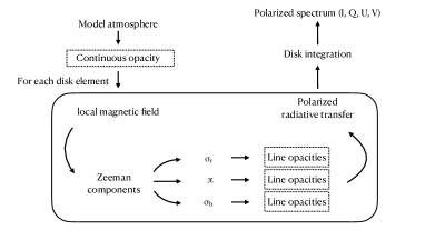
Figure 1: Schematic of the ZeeTurbo implementation.

ZeeTurbo was implemented on the latest published version of Turbospectrum (version 20, with NLTE capabilities, Gerber et al., 2022). Most modifications of the Turbospectrum code where kept in separate routines and files whenever possible. Consequently, the modification to the code mostly affects the bsyn.f file of the Turbospectrum source code. We implemented a trigger to bypass any added feature and use the original Turbospectrum functions only. Currently, ZeeTurbo does not support NLTE computations for line list formatting reasons, but minor modifications to the code will allow us to implement this capability in the future. For the time being, rotation, and macroturbulence are applied as post-processing steps by convolving the spectra with rotation or macroturbulence profiles (Gray, 1975, 2005). In this work, we focus on the analysis of Stokes $I$ spectra, although ZeeTurbo is also able to compute Stokes $Q$, $U$ and $V$ spectra. The analysis of polarised spectra will be treated in subsequent studies.

3.2 Verification and validation

In order to ensure that the spectra synthesised with ZeeTurbo are reliable, we compared them to those computed with Turbospectrum and Zeeman. We find that ZeeTurbo and Turbospectrum produce similar spectra when no magnetic field is considered. The Zeeman and Turbospectrum codes, however, were found to produce significantly different outputs, both in the continuum levels and in the shape of spectral lines. These discrepancies are particularly obvious at temperatures lower than 3500 K. In order to ensure that ZeeTurbo produces Zeeman patterns in agreement with the Zeeman code, we synthesised spectra at higher temperatures (e.g.  6000 K, see Fig. 2) and compared the Zeeman patterns modelled by both codes. We found that the Zeeman patterns computed with ZeeTurbo are consistent with those computed with the Zeeman code. Several comparisons allowed us to validate that ZeeTurbo behaves as expected (see Fig. 2 for an example).

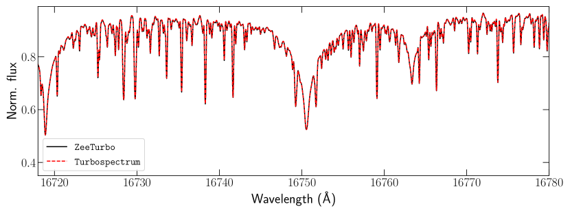
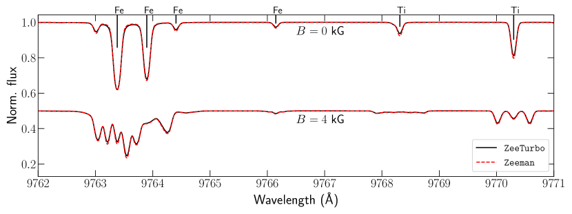
Figure 2: Top panel: comparison between spectra computed for a 0 kG field with ZeeTurbo and Turbospectrum for models with $T_{\rm eff}=3500$ K, $\log g=5.0$ dex, $\rm{[M/H]}=0.0$ dex, and $\rm{[\alpha/Fe]}=0.0$ dex. Bottom panel: comparison between spectra computed with ZeeTurbo and Zeeman for $T_{\rm eff}=6000$ K, $\log g=5.0$ dex, $\rm{[M/H]}=0.0$ dex, and $\rm{[\alpha/Fe]}=0.0$ dex. The spectra were computed assuming that the magnetic field is radial in all points of the photosphere.

3.3 Computing a grid of synthetic spectra with ZeeTurbo

We computed a new grid of synthetic spectra with ZeeTurbo for the analysis of our 6 M dwarfs. The parameters covered by our grid are presented in Table 1. This grid was extended to cover lower temperatures than in our previous studies (Cristofari et al., 2022a, b) in order to analyse cooler targets. All models are computed assuming that the magnetic field is radial and of equal strength for all surface grid cells. Our coverage in $T_{\rm eff}$, $\log g$, $\rm{[M/H]}$, and $\rm{[\alpha/Fe]}$ is expected to be sufficient for most stars observed in the context of the SLS, and the step and span in magnetic field strengths are inspired from previous studies (e.g., Kochukhov & Reiners, 2020; Reiners et al., 2022).

Table 1: Coverage and step size of the computed grid of ZeeTurbo spectra.

$T_{\rm eff}$ (K)	2700 – 4000 (100)
$\log g$ (dex)	4.0 – 5.5 (0.5)
$\rm{[M/H]}$ (dex)	$-1.0$ – $+1.0$ (0.5)
$\rm{[\alpha/Fe]}$ (dex)	$-0.25$ – $+0.50$ (0.25)
$B$ (kG)	0 – 10 (2)

4 Characterising M dwarfs with ZeeTurbo

4.1 Modelling magnetic activity – filling factors

Following the results of previous studies (Shulyak et al., 2010, 2014; Kochukhov & Reiners, 2020; Reiners et al., 2022), we choose to model the stellar spectra as a combination of spectra computed for various magnetic field strengths. This allows us to obtain better fits of the observed spectra by assuming a simple N-component model (with magnetic and non-magnetic regions at the surface of the star). Considering the spectrum $S_{X}$ computed with a field of $X$ kG, the modelled spectrum $S$ is then

$$S=a_{0}S_{0}+a_{2}S_{2}+a_{4}S_{4}+a_{6}S_{6}+a_{8}S_{8}+a_{10}S_{10}$$ (1)

where $a_{X}$ is the filling factor for the field of $X$ kG, verifying that $a_{0}+a_{2}+a_{4}+a_{6}+a_{8}+a_{10}=1$ with all $a_{X}\geq 0$.

Modelling the spectrum then amounts to finding the filling factors that lead to the best fit to our observations.

4.2 Analysis

4.2.1 Constraining atmospheric parameters and magnetic fields

Our analysis is inspired by Cristofari et al. (2022a, b), searching for the model that provides the best fit to observations. However, unlike our previous studies, we now carry out a MCMC analysis, relying on the emcee package (Foreman-Mackey et al., 2013) to estimate the atmospheric parameters from posterior distributions. Prior to their comparison to observations, synthetic spectra are broadened to account for instrumental resolution, macroturbulence and rotation, and shifted to match the observed radial velocity. We then perform an adjustment of the continuum following the steps described in Cristofari et al. (2022b). Fixing both the instrumental width and either the macroturbulence or the rotation velocity to their known values, we end up with 11 parameters to be estimated with our MCMC process. Macroturbulent velocity and rotation are typically difficult to disentangle due to the similar effect they have on spectral lines (see e.g. Gray, 2005; Valenti & Fischer, 2005). In the present paper, we chose to set the value of $v\sin{i}$ and fit the macroturbulent velocity. We found that fixing macroturbulence and fitting the rotational velocity lead to very similar results in atmospheric parameters and magnetic field strengths.

Priors set on atmospheric parameters are meant to prevent walkers to run outside the boundaries of our grid. Priors are also set to ensure that the filling factors remain positive. To ensure that the sum of the filling factors is one, we compute $a_{0}=1-(a_{2}+a_{4}+a_{6}+a_{8}+a_{10})$. For each walker, if one of the filling factors differs from 1, or if the atmospheric parameters fall out of the grid, we set the likelihood value to -infinity.

4.2.2 Deriving error bars

Error bars on atmospheric parameters and filling factors are estimated from posterior distributions. In practice, we find that the minimum reduced $\chi^{2}$ ($\chi^{2}_{\rm r,min}$) derived from fitting the observed spectrum is larger than 1, because of systematic differences between the model and observations, which impacts the results of our MCMC analysis. In order to overcome the issue, we artificially expand the error bars on each pixel by $\sqrt{\chi^{2}_{\rm r,min}}$ before running our analysis, to ensure that the best fit corresponds to a unit $\chi^{2}_{\rm r}$. The factor used to expand the error bars is estimated after a preliminary run.

In our previous work (Cristofari et al., 2022a), formal error bars on atmospheric parameters were found to be smaller than the dispersion between parameters derived using different grids of synthetic spectra. Following  Cristofari et al. (2022a, b) we chose to further enlarge these errors again by quadratically adding to our formal error bars 30 K for $T_{\rm eff}$, 0.05 dex for $\log g$, 0.10 dex for $\rm{[M/H]}$ and 0.04 dex in $\rm{[\alpha/Fe]}$. The resulting error bars are referred to as ‘empirical error bars’ in the rest of the paper.

4.3 Line list

For this analysis, we start from the same atomic and molecular line list used in Cristofari et al. (2022b), adding several Ti, K, and Mg lines included in previous studies (Kochukhov & Reiners, 2020; Reiners et al., 2022), and shown to be useful for estimating magnetic fields. Atomic data, including Landé factors, were extracted from the VALD database (Piskunov et al., 1995; Kupka et al., 2000; Ryabchikova et al., 2015; Pakhomov et al., 2019). For a few Ti lines, corrections to the Van Der Waals parameters were applied following Cristofari et al. (2022b). Data for molecular lines was compiled from Burrows et al. (2002), Barber et al. (2006), Yadin et al. (2012), Sneden et al. (2014), Masseron et al. (2014), Brooke et al. (2016), the ExoMol database (Yadin et al., 2012; Barton et al., 2013; Yurchenko et al., 2018; Tennyson et al., 2020), and the HITRAN database (Rothman et al., 2013; Gordon et al., 2017). Our line list also contains a number of OH and CO lines, assumed to be insensitive to magnetic fields. This assumption was supported by comparing the spectra of weakly and strongly magnetic targets, as well as by the results of previous studies (e.g. López-Valdivia et al., 2021). The lines used in the present analysis are listed in Table 2.

Table 2: List of lines used for our analysis. The identification relied on wavelengths and depths extracted from the VALD database. Effective Landé factors are given for atomic lines. For each atomic line in the table, if two values of effective Landé factors are given, the first is that listed in the VALD database, and the second was computed assuming LS coupling. When effective Landé factors were missing from the VALD database, we display a single value computed assuming LS coupling.

Species	Wavelength (Å) [effective Landé factor]
Ti I	9678.20 [1.35 – 1.35], 9708.33 [1.26 – 1.25], 9721.63 [0.95 – 1.00],
	9731.07 [1.00 – 1.00], 9746.28 [0.00 – 0.00], 9785.99 [1.48 – 1.50],
	9786.27 [1.49 – 1.50], 9790.37 [1.50 – 1.50], 22217.28 [2.08 – 2.00],
	22238.91 [1.66 – 1.67], 22280.09 [1.58 – 1.58],
	22316.70 [2.50 – 2.50], 22969.60 [1.11 – 1.10],
Fe I	10343.72 [0.68 – 0.67],
Mg I	10968.42 [1.33], 15044.36 [1.75], 15051.83 [2.00],
K I	12435.67 [1.33], 12525.56 [1.17], 15167.21 [1.07 – 1.07],
Mn I	12979.46 [1.21 – 1.21],
Al I	13127.00 [1.17], 16723.52 [0.83], 16755.14 [1.10],
Na I	22062.42 [1.17], 22089.69 [1.33],
OH	16073.91, 16539.10, 16708.92, 16712.08,
	16753.83, 16756.30, 16907.35, 16908.89,
	16910.25,
CO	22935.23, 22935.29, 22935.58, 22935.75,
	22936.34, 22936.63, 22937.51, 22937.90,
	22939.09, 22939.58, 22941.09, 22943.49,
	22944.16, 22946.31, 22947.06, 22949.54,
	22950.36, 22953.19, 22954.06, 22957.26,
	22958.16, 22961.74, 22962.67, 22966.65,
	22967.58, 22971.97, 22972.88, 22977.72,
	22978.60, 22983.89, 22984.71, 22990.49

4.4 Benchmarking ZeeTurbo

4.4.1 Building model templates

We ran a benchmark, to ensure that our new tool is indeed capable of constraining atmospheric parameters and filling factors. To this end, we generated a set of model template spectra as follows. From a set of atmospheric parameters and filling factors, we computed a synthetic spectrum. We then broadened this spectrum with a Gaussian profile of full width at half maximum (FWHM) 4.3 $\rm km\,s^{-1}$ to account for the instrumental width of SPIRou, and optionally applied convolution with rotation and/or macroturbulence profiles. The spectrum was then convolved with a 2 $\rm km\,s^{-1}$-wide rectangular function representing pixels, and re-sampled on a typical SPIRou wavelength solution. Noise was added to the spectrum, accounting for the typical SPIRou throughput (Donati et al., 2020) and the typical blaze function for a SPIRou observation. The modelled spectrum, therefore, resembles template spectra in that the noise varies throughout each order, and from order to order.

4.4.2 Simulating the estimation of the atmospheric parameters and filling factors.

We performed our analysis on 50 modelled templates computed for the same atmospheric parameters and filling factors but different noise realisations with the process described in Sec. 4.2. The modelled templates were computed assuming an SNR in the H band of $\sim$500, $T_{\rm eff}=3400$ K, $\log g=5.0$ dex, $\rm{[M/H]}=0.0$ dex and $\rm{[\alpha/Fe]}=0.0$ dex. We set the filling factors of the models to $a_{0}$=0.10, $a_{2}$=0.50, $a_{4}$=0.25, $a_{6}$=0.05, $a_{8}$=0.10 and $a_{10}=0.00$ ( yielding an average magnetic field strength $<\!B\!>=3.1$ kG), thus adopting values consistent with typically observed targets (see Sec. 5). We simultaneously constrained atmospheric parameters and filling factors and analysed posterior distributions to find out potential correlations and estimate uncertainties. Figure 4 presents the results of our benchmark. We find that the dispersion on the series of 50 points is not fully consistent with our formal error bars, especially for the atmospheric parameters $T_{\rm eff}$, $\log g$, $\rm{[M/H]}$ and $\rm{[\alpha/Fe]}$, the reduced $\chi^{2}$ ($\chi^{2}_{\rm r}$) on the residuals (the retrieved parameters minus the median) reaching up to $3.2$. Subsequent tests showed that most of this excess dispersion can be attributed to the continuum adjustment step. We also find that the effect of the continuum adjustment is sensitive to the SNR, and can introduce systematic offsets in the retrieved atmospheric parameters of up to 0.01 dex in $\log g$ or $\rm{[M/H]}$ and up to 0.5 K in $T_{\rm eff}$ with a SNR $\sim$500. These shifts reach up to 20 K in $T_{\rm eff}$ and 0.1 dex in $\log g$, $\rm{[M/H]}$ and $\rm{[\alpha/Fe]}$ if we assume a SNR $\sim$100. In practice, the SPIRou templates usually reach an SNR in the $H$ band of $\sim$2000, implying that our results should not be affected by such biases.

With our benchmark, we explored the impact of magnetic fields on the estimation of atmospheric parameters. We generated templates for magnetic stars, and ran our analysis with non-magnetic models. The recovered atmospheric parameters deviate from the input parameters by up to 30 K in $T_{\rm eff}$ and 0.3 dex $\log g$ (see Fig. 5) for this particular magnetic configuration. Smaller biases ($<0.1$ dex) are found on $\rm{[M/H]}$ and $\rm{[\alpha/Fe]}$. These systematic shifts can be $\sim$10 times larger than our formal error bars for large values of the magnetic flux.

4.4.3 Estimating field strengths from known magnetic configurations

We carried out additional simulations to assess the precision at which field strengths are recovered given the a priori assumptions of our model, in particular on the field topology; we achieve this by running our tool on synthetic spectra of a star with a known magnetic configuration.

We consider a star hosting an 8 kG dipolar magnetic field inclined at 90^∘ with respect to the rotation axis, for a star viewed equator on. We computed synthetic spectra for 10 evenly spaced rotation phases. We added noise to each spectra and ran our analysis at each phase. We then compared the retrieved average magnetic field strengths (${<\!B\!>}$) to the true field strengths averaged over the visible hemisphere of the star ($B_{\rm s}$, see Fig. 3). We find that $<\!B\!>$ is in good agreement with $B_{\rm s}$, though slightly smaller by about 3-4% (i.e. 0.15-0.25 kG). This slight difference comes from our modelling assumption that the field is radial over the whole surface.

We also performed our analysis on a spectrum obtained by taking the median of the spectra at all phases. The average magnetic field obtained with the median spectrum is 5.5 kG, consistent with the median of the retrieved $<\!B\!>$ values.

Altogether, it demonstrates that our modeling assumptions are quite reasonable and introduce only marginal biases in the measured field strengths.

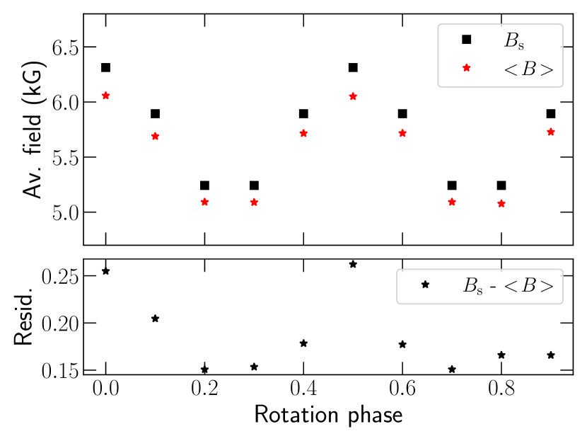
Figure 3: Magnetic field strengths for a rotating star hosting a 8 kG dipole whose axis is perpendicular to the rotation axis. For each rotation phase, we compare the average magnetic strength recovered with our analysis ($<\!B\!>$, red stars) to the true magnetic field averaged over the visible hemisphere of the star ($B_{\rm s}$, black squares). The bottom panel shows the residuals.

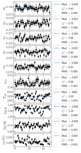
Figure 4: Example of comparison between input and output parameters. The blue horizontal solid line marks the median. For each parameter, we compute the $\chi^{2}$ of the series of points. The models were computed for $T_{\rm eff}=3400$ K, $\log g=5.0$ dex, $\rm{[M/H]}=0.00$ dex and $\rm{[\alpha/Fe]}=0.00$ dex.

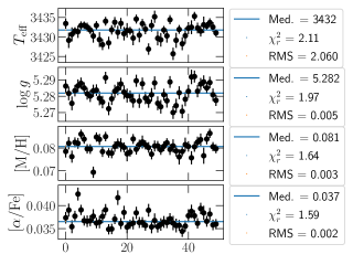
Figure 5: Same as Fig. 4 but with no magnetic field considered for the analysis.

5 Application to SPIRou spectra

We applied our new tool to our template SPIRou spectra of AU Mic, AD Leo, EV Lac, DS Leo, CN Leo and PM J18482+0741, relying on models computed for magnetic fields ranging from 0 to 10 kG in steps of 2 kG.

For the coolest targets in our sample (CN Leo and PM J18482+0741), we found discrepancies between the best-fitted model and the SPIRou template for some lines, such as the Ti line at 9678 Å (see Fig. 6). We worked out that the presence of spurious TiO lines in the synthetic spectra were responsible for some of these discrepancies, and that removing this molecule from the spectral synthesis improved the fit quality for the coolest stars in our sample. The results presented in this section were obtained with synthetic spectra computed without TiO, after checking that very similar results (and worse fits) were obtained when keeping TiO in.

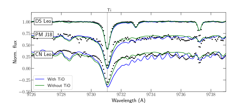
Figure 6: Best obtained fit with synthetic spectra computed with and without TiO for the two coolest stars in our sample (CN Leo and PM J18482+0741) and DS Leo. The black points show the SPIRou templates.

The label of PM J18482+0741 was abbreviated PM J18 for better readability.

Table 3: Literature parameters for the stars in our sample. For all stars but AU Mic, masses were obtained from the mass-$K$ band magnitude proposed by Mann et al. (2019), and radii were computed from the mass with the models of Baraffe et al. (2015) assuming an age of 5 Gyr for all stars but AU Mic. $K$ band magnitudes were extracted from the SIMBAD database (Wenger et al., 2000). For each star, we report $v\sin{i}$ estimates from the literature, or our adopted values if rotation period and radius estimates suggested that the literature $v\sin{i}$ was overestimated. The convective turnover time ($\tau$) is taken from Reiners et al. (2022). The Rossby number ($R_{\rm O}$) is computed from the rotation period ($P_{\rm rot}$) and $\tau$. Ref. – a: Plavchan et al. (2020), b: Donati et al., (submitted), c: Gallenne et al. (2022), d: Morin et al. (2008), e: Díez Alonso et al. (2019a), f: Donati et al. (2008) g: Reiners et al. (2018) h: Reiners & Basri (2007).

Star	GJ ID	Spectral type	$P_{\rm rot}$ (d)	$M$ ($M_{\sun}$)	$R$ ($R_{\sun}$)	$v\sin{i}$ ($\rm km\,s^{-1}$)	$\tau$ (d)	$R_{\rm O}$
AU Mic	Gl 803	M1V	$4.863\pm 0.010^{\textit{a}}$	$0.60\pm 0.03^{\textit{b}}$	$0.82\pm 0.05^{\textit{b }}$	$8.5\pm 1.0^{\textit{b}}$	39	$0.125$
EV Lac	Gl 873	M4.0V	$4.3715\pm 0.0006^{\textit{d}}$	$0.32\pm 0.02$	$0.31\pm 0.02$	$3\pm 1$	110	$0.040$
AD Leo	Gl 388	M3V	$2.2399\pm 0.0006^{\textit{d}}$	$0.42\pm 0.02$	$0.39\pm 0.02$	$3\pm 1^{\textit{d}}$	80	0.028
CN Leo	Gl 406	M6V	$2.704\pm 0.003^{\textit{e}}$	$0.11\pm 0.02$	$0.13\pm 0.02$	$2\pm 1$	387	0.007
PM J18482+0741	–	M5.0V	$2.76\pm 0.01^{\textit{e}}$	$0.14\pm 0.02$	$0.17\pm 0.02$	$2.4\pm 1.5^{\textit{g}}$	230	0.012
DS Leo	Gl 410	M1.0V	$14.0\pm 0.1^{\textit{f}}$	$0.57\pm 0.02$	$0.53\pm 0.02$	$1.5\pm 1.0$	60	0.233

5.1 AU Mic = Gl 803

The young planetary system AU Mic attracted significant attention in the recent years (Boccaletti et al., 2018; Kochukhov & Reiners, 2020; Martioli et al., 2020; Martioli et al., 2021; Klein et al., 2021, 2022) and has been monitored by several instruments.

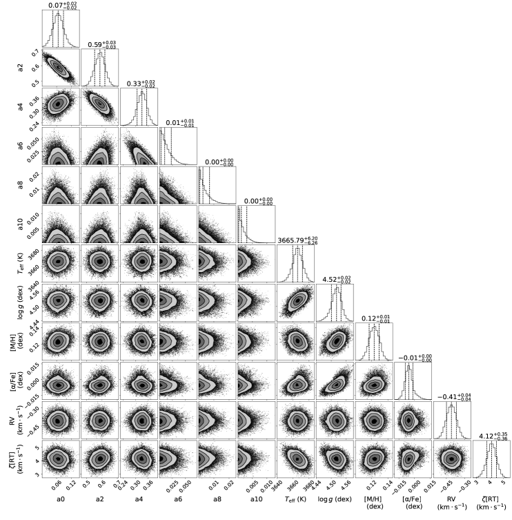
Figure 7: Corner plot presenting posterior distributions for filling factors and atmospheric parameters for AU Mic.

The rotation period of this star is ${P_{\rm rot}=4.863\pm 0.010}$ d (Plavchan et al., 2020; Klein et al., 2021) with an angle between the line of sight and the rotation axis close to $90^{\circ}$, and its radius was estimated from interferometric measurements to $0.862\pm 0.052~{}{\rm R_{\sun}}$ (Gallenne et al., 2022). For this star, we adopt a $v\sin{i}=8.5\pm 1.0$ $\rm km\,s^{-1}$ (Donati et al., in prep), yielding a radius of $0.82~{}{\rm R_{\sun}}$. With a mass estimated at $0.60\pm 0.03~{}{\rm M_{\sun}}$ (Donati et al., in prep), the logarithmic surface gravity of AU Mic is then equal to $\log g=4.39$ dex.

We performed an analysis of AU Mic fitting $\zeta_{\rm RT}$ and fixing $v\sin{i}=8.5$ $\rm km\,s^{-1}$ (see Table 4). From posterior distributions, we estimate a $T_{\rm eff}=3665\pm 31$ K, $\log g=4.52\pm 0.05$ dex, $\rm{[M/H]}=0.12\pm 0.10$ dex and $\rm{[\alpha/Fe]}=0.00\pm 0.04$ dex. These estimates are listed Table 4. The temperature is consistent with that estimated from SEDs (Afram & Berdyugina, 2019). Our $\log g$ is significantly larger than that estimated from mass and radius. We attempted to perform the analysis by fixing the value of $\log g$ to 4.40 dex. In that case, we retrieve a $T_{\rm eff}=3641\pm 31$ K and $\rm{[M/H]}=0.06\pm 0.10$ dex, and $\zeta_{\rm RT}=5.4\pm 0.2$ $\rm km\,s^{-1}$, still consistent with literature values.

The derived filling factors amount to an average field strength $<\!B\!>=2.61\pm 0.05$ kG (see Fig. 9), which compares well to values reported in the literature of, for example, 2.1–2.3 kG (Kochukhov & Reiners, 2020) and $3.01\pm 0.22$ kG (Reiners et al., 2022). When fixing $\log g$ to 4.40 dex, the average field strength rises up to ${<\!B\!>=2.68\pm 0.05}$ kG, still consistent with the values reported in the literature.

We repeated our analysis assuming a Gaussian macroturbulence. With this kernel, we recovered $T_{\rm eff}$, $\log g$, $\rm{[M/H]}$, $\rm{[\alpha/Fe]}$ and $<\!B\!>$ very close to those assuming a radial-tangential macroturbulence profile (see Table 4). The strong constraint derived for $<\!B\!>$ can be explained by the dependence of line shapes on the magnetic field, as illustrated in Fig. 8 and Fig. B1 (available as supplementary material). We note that the filling factors $a_{2}$ and $a_{4}$ associated with the 2 and 4 kG components account for most of the surface field of AU Mic (see Fig. 9). To diagnose the influence of the higher-field components on the results, we performed a second analysis, omitting the 8 and 10 kG models. We find no change in the atmospheric parameters, and that the average magnetic field is lowered by a negligible amount, with a difference of 0.01 kG on $<\!B\!>$, thus confirming that keeping the 8 and 10 kG components do not generate additional errors when characterizing the surface magnetic field of AU Mic.

We also applied our analysis on spectra recorded for each night (Donati et al., submitted). As in our simulation (see Sec. 4.4.3), we find that the average magnetic field strength derived from the SPIRou template is consistent with the median of the field strengths derived for each night. These results provide further evidence that analysing median spectra does not introduce biases in the derived magnetic field strengths.

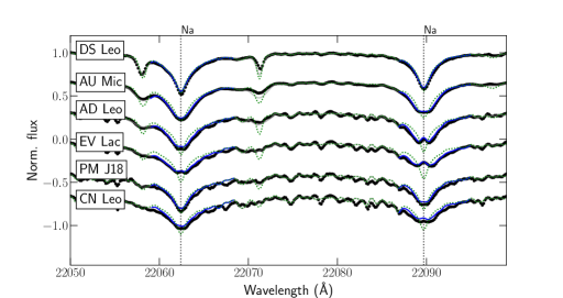
Figure 8: Best fit obtained for the seven stars included in our study with ZeeTurbo for two Na lines (22062.4 and 22089.7 Å). Black points present the data. The grey solid line shows the best fit, and the blue solid blue line presents the part of the windows used for the fit. The green dotted line shows the model obtained for the same atmospheric parameters but with a zero magnetic field. The name PM J18482+0741 was replaced by PM J18 for better readability.

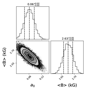
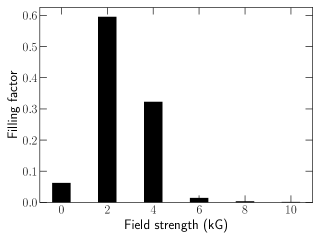
Figure 9: Left panel: non-magnetic component against average field strength for AU Mic. Right panel: distribution of the filling factors over magnetic field components for AU Mic.

5.2 AD Leo = Gl 388

We performed a similar analysis on AD Leo (Gl 388). This star was included in the sample of previous studies studies (Morin et al., 2008; Reiners et al., 2022), and its projected rotational velocity was estimated to $v\sin{i}=3\pm 1$ $\rm km\,s^{-1}$ (Morin et al., 2008). The mass and radius of this star were estimated from the mass-K band magnitude relation of (Mann et al., 2019) and the models of (Baraffe et al., 2015) (see Table 3). These yield a $\log g\sim 4.88\pm 0.05$ dex. The rotation period of AD Leo is $P_{\rm rot}=2.2399\pm 0.0006$ d (Morin et al., 2008, see Table 3).

We chose to fix the value of $v\sin{i}$ and fit a radial-tangential macroturbulence in this analysis. With these constraints, we derive an average magnetic field of $3.03\pm 0.06$ kG, consistent with some previous estimates, e.g. $2.9\pm 0.2$ kG (Reiners & Basri, 2007) and $3.57\pm 0.09$ kG (Reiners et al., 2022). Just like for AU Mic, we find the largest filling factors for the 2 and 4 kG components for this star. The retrieved atmospheric parameters, i.e. $T_{\rm eff}=3467\pm 31$, $\log g=4.90\pm 0.05$, $\rm{[M/H]}=0.24\pm 0.10$ and $\rm{[\alpha/Fe]}=0.00\pm 0.04$ compare well with previous estimates (Mann et al., 2015), with the exception of a few recent studies suggesting that this star may be metal-poor (Marfil et al., 2021). Our $\log g$ is in good agreement with the mass and radius estimates.

With $v\sin{i}=3$ $\rm km\,s^{-1}$, we retrieve a radial-tangential macroturbulence $\zeta_{\rm{RT}}=1.7\pm 0.2$ $\rm km\,s^{-1}$. We repeat the analysis, this time with a Gaussian macroturbulence, and retrieve a FWHM of $\zeta_{\rm G}=2.0\pm 0.2$ $\rm km\,s^{-1}$. We find that changing the macroturbulence model has a negligible impact on the derived atmospheric parameters and filling factors (see Table 4).

5.3 EV Lac = Gl 873

EV Lac (Gl 873) is another very well-known magnetic M dwarf observed in the context of the SLS, with a rotation period of ${P_{\rm rot}=4.3715\pm 0.0006}$ d (Morin et al., 2008). We estimated its mass and radius to $M=0.32\pm 0.02~{}{\rm M_{\sun}}$ and $R=0.31\pm 0.02~{}{\rm R_{\sun}}$ (see Table 3), thus implying $\log g=4.96\pm 0.06$ dex. The projected rotational velocity of this star was estimated to about $4\pm 1$ $\rm km\,s^{-1}$ (Morin et al., 2008). The radius and rotation period of this star would suggest that this value is slightly over-estimated, and we therefore choose to fix its value to $v\sin{i}=3$ $\rm km\,s^{-1}$.

We fixed $v\sin{i}$, and fitted the radial-tangential macroturbulent velocity $\zeta_{\rm RT}$. For this star we derive ${T_{\rm eff}=3340\pm 31}$ K, ${\log g=4.87\pm 0.05}$ dex, ${\rm{[M/H]}=0.04\pm 0.10}$ dex and ${\rm{[\alpha/Fe]}=0.01\pm 0.04}$ dex. These atmospheric parameters are in good agreement with those reported by previous studies (Maldonado et al., 2020). Our $\log g$ estimate is also in good agreement with the estimated mass and radius for this star. We compute an average magnetic field of $<\!B\!>=4.53\pm 0.07$ kG, consistent with estimates reported in the literature, of $3.8\pm 0.5$ kG (Johns-Krull & Valenti, 2000) or $4.32\pm 0.11$ kG (Reiners et al., 2022). For this star, we note that the filling factors associated to the 6, 8 and 10 kG components are not close to 0, but rather account for 30 % of the total magnetic flux (see Fig. 12).

We retrieved a macroturbulent velocity $\zeta_{\rm RT}=4.2\pm 0.2$ $\rm km\,s^{-1}$. We repeat the analysis, this time fitting a Gaussian macroturbulence model, and retrieve a FWHM of $\zeta_{\rm G}=4.6\pm 0.3$ $\rm km\,s^{-1}$. We further checked that changing the adopted value of $v\sin{i}$ by 1 $\rm km\,s^{-1}$ had negligible impact on the retrieved atmospheric parameters and magnetic field strength. Here again, the choice of model for the macroturbulence profile has negligible impact on the derived atmospheric parameters and magnetic field strength (see Table 4).

5.4 CN Leo = Gl 406

We then performed our analysis on the SPIRou template of CN Leo (Gl 406), an active late-type M dwarf. The rotation period of this star is ${P_{\rm rot}=2.704\pm 0.003}$ d (Díez Alonso et al., 2019a), and we estimate its mass and radius to $M=0.11\pm 0.02~{}{\rm M_{\sun}}$ and $R=0.13\pm 0.02~{}{\rm R_{\sun}}$ (see Table 3). The projected rotational velocity of CN Leo was previously estimated to $v\sin{i}=3\pm 1$ $\rm km\,s^{-1}$ (Reiners & Basri, 2007). Given the rotation period and radius for this star, we find that $v\sin{i}=3$ $\rm km\,s^{-1}$ is likely overestimated, and we chose to fix its value to $v\sin{i}=2$ $\rm km\,s^{-1}$.

We retrieve $T_{\rm eff}=2898\pm 31$ K, in good agreement with previously reported estimates (Mann et al., 2015). Our estimate of $\log g=4.82\pm 0.08$ dex is significantly lower than that computed from mass and radius, of $\log g=5.25\pm 0.17$ dex. We derive $\rm{[M/H]}=0.17\pm 0.12$ dex, consistent with previous estimates (Rojas-Ayala et al., 2012; Mann et al., 2015).

We recover an average magnetic field strength $<\!B\!>=3.45\pm 0.20$ kG, consistent with previously reported values ($<\!B\!>=3.01\pm 0.16$ kG, Reiners et al., 2022). Again, we find that fitting the data with a Gaussian macroturbulence profile yields almost identical parameters (see Table 4).

5.5 PM J18482+0741

PM J18482+0741 is another cool M dwarf observed in the context of the SLS, with a projected rotational velocity estimated to $v\sin{i}=2.4\pm 1.5$ $\rm km\,s^{-1}$ (Reiners et al., 2018), and a mass and radius estimated to ${M=0.14\pm 0.02~{}{\rm M_{\sun}}}$ & ${R=0.17\pm 0.02~{}{\rm R_{\sun}}}$ (see Table 3), yielding $\log g=5.12\pm 0.13$ dex. The rotation period of this star was estimated by (Díez Alonso et al., 2019b) to $2.76\pm 0.01$ d.

For this target, we retrieve $T_{\rm eff}=3078\pm 32$ K, consistent with previously reported effective temperatures for this target (Gaidos et al., 2014; Passegger et al., 2019). Our recovered $\log g=4.72\pm 0.06$ is lower than that reported by (Passegger et al., 2019) and that implied by our radius and mass estimates. With our process, we retrieve an average magnetic field $<\!B\!>=1.99\pm 0.15$ kG, almost twice that of Reiners et al. (2022, $<\!B\!>=1.19\pm 0.23$ kG). We find that for this star too, fitting the data with a Gaussian instead of a radial-tangential macroturbulence profile has negligible impact on the results (see Table 4).

DS Leo = Gl 410

Finally, we run our process on the moderately active DS Leo (Gl 410). The rotation period of this star, of $P_{\rm rot}=14\pm 0.1$ d (Donati et al., 2008), is the largest in our sample. The mass and radius of DS Leo, estimated to $M=0.57\pm 0.02~{}{\rm M_{\sun}}$ and $R=0.53\pm 0.02~{}{\rm R_{\sun}}$ (see Table 3), implies a surface gravity of $\log g=4.74\pm 0.04$ dex. For this star, $v\sin{i}$ was estimated to $2\pm 1$ $\rm km\,s^{-1}$ by Morin et al. (2008).

With a fixed value of $v\sin{i}$, we retrieved ${T_{\rm eff}=3818\pm 30}$ K, $\log g=4.79\pm 0.05$ dex, $\rm{[M/H]}=0.01\pm 0.10$ dex and ${\rm{[\alpha/Fe]}=0.03\pm 0.04}$ dex (see Table 4). These values are in good agreement with previous estimates, including ours (Mann et al., 2015; Cristofari et al., 2022b). Our $\log g$ is also comparable to that implied by previous mass and radius estimates. We derive $<\!B\!>=0.73\pm 0.03$ kG, lower than that reported by Reiners et al. (2022), of $<\!B\!>=1.04\pm 0.06$ kG. For DS Leo, we find $a_{4}$, $a_{6}$ and $a_{8}$ to be close to 0. We repeat our analysis process, only using models computed for 0 and 2 kG, and find that removing the 4, 6, 8 and 10 kG components has negligible impact on the estimation of atmospheric parameters and filling factors.

5.6 Comparison with the literature

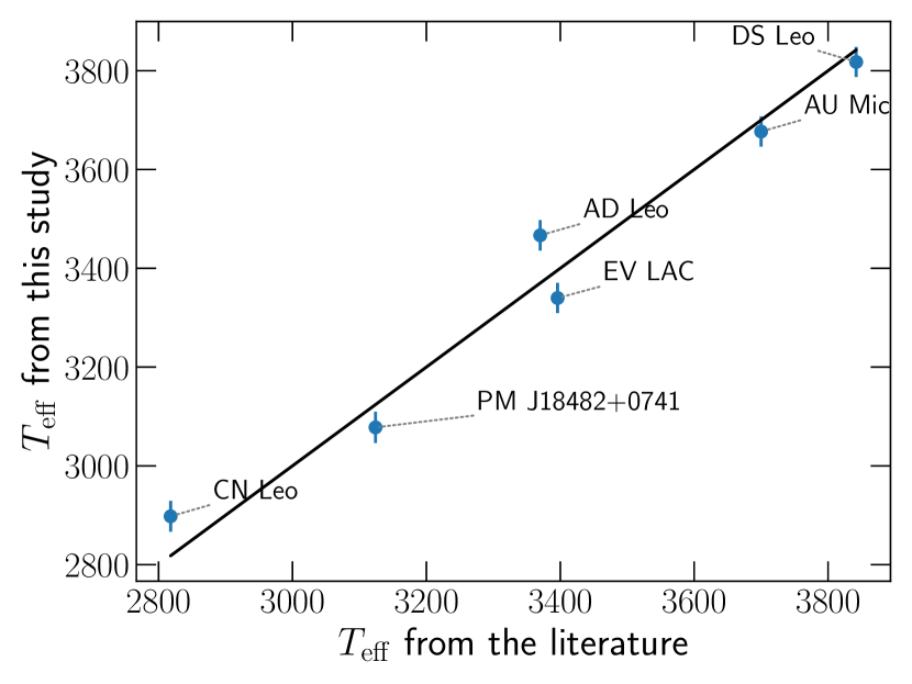
Figure 17: Retrieved $T_{\rm eff}$ compared to literature estimates taken from Afram & Berdyugina (2019, AU Mic), Mann et al. (2015, AD Leo, CN Leo), Maldonado et al. (2020, EV Lac), Cristofari et al. (2022b, DS Leo) and Passegger et al. (2019, PM J18482+0741).

Figure 10 presents a comparison between our retrieved $<\!B\!>$ estimates and those reported by Reiners et al. (2022). We find an overall good agreement between the two sets of values. $<\!B\!>$ is expected to evolve with time, which can at least partly account for some of the observed differences. Figure 11 presents the position of the stars in a $<\!B\!>$ vs Rossby number ($R_{\rm O}$) diagram. Most active M dwarfs included in our sample fall within the saturated dynamo regime, with the exception of DS Leo. These results are also in good agreement with those reported in Reiners et al. (2022). Comparisons between our retrieved $T_{\rm eff}$, $\log g$ and literature estimates are presented in Figs. 17 & 18.

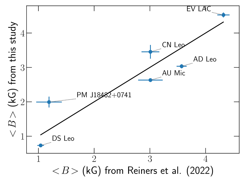
Figure 10: Comparison between our derived $<\!B\!>$ values and those of Reiners et al. (2022). The black line marks the equality

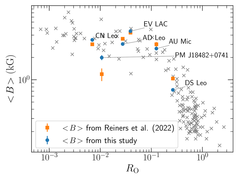
Figure 11: Comparison Rossby number ($R_{\rm O}$) and $<\!B\!>$ values derived from our study (blue dots) and reported by Reiners et al. (2022, orange squares). The grey symbols mark the position of all the stars studied by Reiners et al. (2022).

Table 4: Retrieved stellar parameter and magnetic fields for our sample of targets. Values given with no associated uncertainties were fixed. For each star, multiple lines present the results obtained when fixing different parameters.

Star (GJ ID) $T_{\rm eff}$ $\log g$ $\rm{[M/H]}$ $\rm{[\alpha/Fe]}$ $v\sin{i}$ $\zeta_{\rm RT}$ $\zeta_{\rm G}$ $<\!B\!>$ $f_{0}$, $f_{2}$, $f_{4}$, $f_{6}$, $f_{8}$, $f_{10}$ AU Mic (Gl 803) $3665\pm 31$ $4.52\pm 0.05$ $0.12\pm 0.10$ $0.00\pm 0.04$ $8.5$ $4.1\pm 0.3$ – $2.61\pm 0.05$ $0.07\pm 0.02$, $0.59\pm 0.03$, $0.33\pm 0.03$, $0.01\pm 0.01$, $0.00\pm 0.00$, $0.00\pm 0.00$ AU Mic (Gl 803) $3666\pm 31$ $4.52\pm 0.05$ $0.12\pm 0.10$ $0.00\pm 0.04$ $8.5$ – $4.7\pm 0.4$ $2.62\pm 0.05$ $0.07\pm 0.02$, $0.59\pm 0.03$, $0.32\pm 0.03$, $0.01\pm 0.01$, $0.00\pm 0.00$, $0.00\pm 0.00$ AU Mic (Gl 803) $3640\pm 31$ $4.40$ $0.10\pm 0.10$ $-0.02\pm 0.04$ $8.5$ $5.1\pm 0.2$ – $2.68\pm 0.05$ $0.06\pm 0.02$, $0.58\pm 0.03$, $0.33\pm 0.03$, $0.01\pm 0.01$, $0.00\pm 0.00$, $0.00\pm 0.00$ AU Mic (Gl 803) $3641\pm 31$ $4.40$ $0.10\pm 0.10$ $-0.02\pm 0.04$ $8.5$ – $6.4\pm 0.4$ $2.68\pm 0.05$ $0.06\pm 0.02$, $0.59\pm 0.03$, $0.33\pm 0.03$, $0.01\pm 0.01$, $0.00\pm 0.00$, $0.00\pm 0.00$ EV LAC (Gl 873) $3340\pm 31$ $4.87\pm 0.05$ $0.04\pm 0.10$ $0.01\pm 0.04$ $3.0$ $4.2\pm 0.2$ – $4.53\pm 0.07$ $0.02\pm 0.04$, $0.29\pm 0.03$, $0.38\pm 0.04$, $0.09\pm 0.04$, $0.13\pm 0.04$, $0.08\pm 0.02$ EV LAC (Gl 873) $3342\pm 31$ $4.88\pm 0.05$ $0.03\pm 0.10$ $0.01\pm 0.04$ $3.0$ – $4.6\pm 0.2$ $4.52\pm 0.07$ $0.02\pm 0.04$, $0.29\pm 0.03$, $0.39\pm 0.04$, $0.09\pm 0.05$, $0.13\pm 0.04$, $0.08\pm 0.02$ AD Leo (Gl 388) $3467\pm 31$ $4.90\pm 0.05$ $0.24\pm 0.10$ $-0.00\pm 0.04$ $3.0$ $1.7\pm 0.2$ – $3.03\pm 0.06$ $0.04\pm 0.02$, $0.50\pm 0.03$, $0.41\pm 0.03$, $0.04\pm 0.02$, $0.01\pm 0.01$, $0.00\pm 0.00$ AD Leo (Gl 388) $3467\pm 31$ $4.89\pm 0.05$ $0.24\pm 0.10$ $-0.01\pm 0.04$ $3.0$ – $2.0\pm 0.3$ $3.04\pm 0.06$ $0.03\pm 0.02$, $0.50\pm 0.03$, $0.41\pm 0.03$, $0.04\pm 0.02$, $0.01\pm 0.01$, $0.00\pm 0.00$ CN Leo (Gl 406) $2898\pm 31$ $4.82\pm 0.08$ $0.17\pm 0.12$ $-0.04\pm 0.04$ $2.0$ $4.3\pm 0.3$ – $3.45\pm 0.20$ $0.10\pm 0.07$, $0.44\pm 0.11$, $0.29\pm 0.10$, $0.07\pm 0.06$, $0.07\pm 0.05$, $0.03\pm 0.03$ CN Leo (Gl 406) $2899\pm 31$ $4.82\pm 0.07$ $0.16\pm 0.11$ $-0.04\pm 0.04$ $2.0$ – $4.8\pm 0.3$ $3.45\pm 0.19$ $0.10\pm 0.07$, $0.44\pm 0.11$, $0.29\pm 0.10$, $0.07\pm 0.06$, $0.07\pm 0.05$, $0.03\pm 0.03$ DS Leo (Gl 410) $3818\pm 30$ $4.79\pm 0.05$ $0.01\pm 0.10$ $0.03\pm 0.04$ $1.5$ $2.7\pm 0.1$ – $0.73\pm 0.03$ $0.65\pm 0.00$, $0.34\pm 0.02$, $0.00\pm 0.00$, $0.00\pm 0.00$, $0.00\pm 0.00$, $0.00\pm 0.00$ DS Leo (Gl 410) $3818\pm 33$ $4.79\pm 0.06$ $0.01\pm 0.10$ $0.03\pm 0.04$ $1.5$ – $3.0\pm 0.3$ $0.82\pm 0.10$ $0.66\pm 0.01$, $0.32\pm 0.04$, $0.01\pm 0.01$, $0.01\pm 0.01$, $0.00\pm 0.00$, $0.00\pm 0.00$ PM J18482+0741 $3078\pm 32$ $4.72\pm 0.06$ $-0.02\pm 0.10$ $-0.05\pm 0.04$ $2.4$ $4.8\pm 0.4$ – $1.99\pm 0.16$ $0.23\pm 0.04$, $0.65\pm 0.09$, $0.08\pm 0.05$, $0.02\pm 0.02$, $0.01\pm 0.01$, $0.01\pm 0.01$ PM J18482+0741 $3081\pm 34$ $4.72\pm 0.08$ $-0.03\pm 0.11$ $-0.05\pm 0.04$ $2.4$ – $5.2\pm 0.5$ $2.08\pm 0.24$ $0.25\pm 0.05$, $0.63\pm 0.13$, $0.07\pm 0.06$, $0.02\pm 0.02$, $0.02\pm 0.02$, $0.01\pm 0.01$

6 Discussion and conclusions

In this paper, we present our first results with our new tools aimed at characterising M dwarfs from SPIRou spectra. Our process relies on the comparison of high-resolution synthetic spectra computed from state-of-the-art MARCS model atmospheres to data, and is used to constrain $T_{\rm eff}$, $\log g$, $\rm{[M/H]}$, $\rm{[\alpha/Fe]}$ and the average magnetic field strengths for 4 targets observed in the context of the SLS.

We introduce a new code, ZeeTurbo, built from the Turbospectrum and Zeeman codes, allowing us to synthesise spectra of magnetic stars from MARCS model atmospheres. We compared the output spectra computed with ZeeTurbo, Zeeman and Turbospectrum and found that our new code allows us to properly synthesise spectra for magnetic M dwarfs. Our code also allowed us to synthesise molecular lines, assumed to be insensitive to magnetic fields in the present work. This assumption holds for the lines our analysis relies on, namely the few OH lines and the CO lines at 2.28 $\mu$m. Modelling molecular lines is particularly critical to the analysis of M dwarfs spectra since they are numerous and blend with atomic features.

With our newly implemented code, we computed a grid of synthetic spectra assuming a constant magnetic field, radial in all points of the photosphere. We modelled the spectra by a linear combination of profiles computed for different magnetic strengths, and fitted our model to SPIRou templates to constrain $T_{\rm eff}$, $\log g$, $\rm{[M/H]}$, $\rm{[\alpha/Fe]}$, the filling factors and thereby the surface magnetic flux. Our analysis relies on a MCMC process, and the atmospheric parameters and filling factors are estimated from posterior distributions. We performed a benchmark, designed to assess the performances of our new tool, and found that it was capable of simultaneously constraining magnetic fields and atmospheric parameters. We also show that our modeling assumptions, e.g. on the field topology, introduce only small biases in the measured field strengths. We then applied our tool to a few well-known magnetic stars observed in the context of the SLS (AU Mic, AD Leo, EV Lac, DS Leo, CN Leo and PM J18482+0741). Our recovered atmospheric parameters and magnetic field estimates are found in good agreement with the literature for most stars. The largest discrepancies between our results and the literature are found for the two coolest stars in our sample (CN Leo and PM J18482+0741), with $\log g$ estimates significantly lower than those computed from masses and radii.

The average surface magnetic flux retrieved with our process for the six targets in our sample are in good agreement with previous estimates reported by Reiners et al. (2022, see Fig. 10). Our estimates are also consistent with most of our stars being in the saturated dynamo regime, with the exception of DS Leo, whose rotation period is significantly longer than that of the other stars. The differences in the values reported in the literature and those derived in this study may partly arise from the evolution of the surface magnetic flux with time.

We find that the way the surface magnetic flux is distributed across the magnetic field strengths differs from star to star. In particular, we find significantly larger contributions of the 6, 8 and 10 kG components for EV Lac of CN Leo, than for the other targets of our sample. For the quietest star in our sample, DS Leo, the best fit relies almost entirely on the 0 and 2 kG components. Moreover, the contribution of the 0 kG component also differs from star to star, and is not necessarily smallest for the most magnetic targets (e.g. the case of CN Leo, where $a_{0}=0.10$, see Fig. 15). These results illustrate the variety of magnetic topologies encountered in our sample, and the possibility to distinguish them using unpolarised spectra. Besides, we find that applying our tool to spectra collected on individual nights (e.g., in the case of AU Mic, Donati et al., submitted) yields field strengths whose median value is consistent with the field strength derived from the median spectrum.

In this work, spectra computed with ZeeTurbo relied on MARCS models that neglect the impact of the additional pressure from magnetic fields on the structure of the atmosphere. Recent works have attempted to obtain improved model atmospheres of magnetic stars (Valyavin et al., 2004; Kochukhov et al., 2005; Shulyak et al., 2010; Stift & Alecian, 2016; Järvinen et al., 2020). Future studies using ZeeTurbo may build up on such improvements.

ZeeTurbo will allow us to analyse all stars observed in the context of the SLS in a self-consistent way. In particular, we will reprocess the M dwarfs included in our previous studies, to measure their surface magnetic fluxes and assess their impact on the atmospheric characterisation. We will also look for temporal evolution in the average magnetic flux of stars monitored over several years, in order to find new means of constraining rotation, activity cycles, and help disentangle activity jitters from radial velocity signals (Haywood et al., 2016; Suárez Mascareño et al., 2020, Donati et al., in prep). We will also expand our analysis to PMS stars, whose modelling may require to account for veiling and starspots, and whose characterisation is essential to the study of stars and planets formation (Flores et al., 2021; López-Valdivia et al., 2021).

Data Availability

The data used in this work were recorded in the context of the SLS, and will be available to the public at the Canadian Astronomy Data Center one year after completion of the program.

Appendix A Additional figures

Figures 12, 13 and 14 present the same plots as Fig. 9 for EV Lac, AD Leo, DS Leo, CN Leo and PM J18482+0741 respectively.

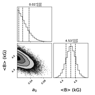
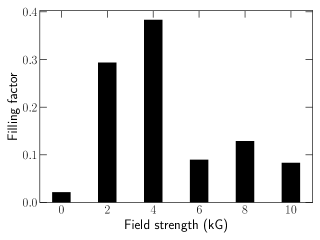
Figure 12: Same as 9 for EV Lac.

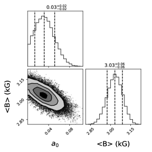
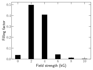
Figure 13: Same as 9 for AD Leo.

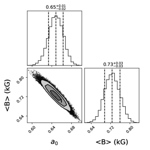
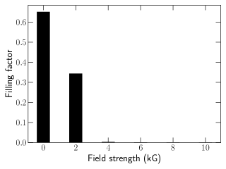
Figure 14: Same as 9 for DS Leo.

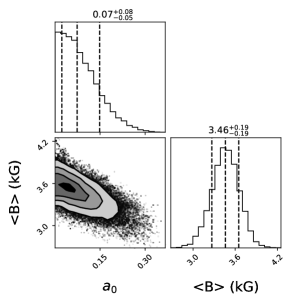
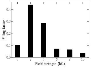
Figure 15: Same as 9 for CN Leo.

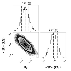
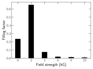
Figure 16: Same as 9 for PM J18482+0741.

Appendix B Best fits

Figure B1 available as supplementary material presents the best fits obtained for AU Mic, AD Leo, EV Lac and DS Leo for all lines used in our analysis.

Appendix C Corner plots

Figures C1-C14, available as supplementary material, present the corner plots obtained for the 6 stars in our sample.

Appendix D Comparison of $T_{\rm eff}$ and $\log g$ with the literature

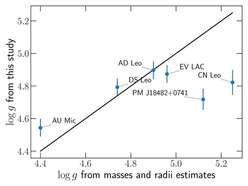
Figure 18: Retrieved $\log g$ compared to estimates derived from masses and radii (see Table 3).

References

- Afram & Berdyugina (2019) Afram N., Berdyugina S. V., 2019, A&A, 629, A83
- Alvarez & Plez (1998) Alvarez R., Plez B., 1998, A&A, 330, 1109
- Baraffe et al. (2015) Baraffe I., Homeier D., Allard F., Chabrier G., 2015, A&A, 577, A42
- Barber et al. (2006) Barber R. J., Tennyson J., Harris G. J., Tolchenov R. N., 2006, MNRAS, 368, 1087
- Barton et al. (2013) Barton E. J., Yurchenko S. N., Tennyson J., 2013, MNRAS, 434, 1469
- Bellotti et al. (2022) Bellotti S., Petit P., Morin J., Hussain G. A. J., Folsom C. P., Carmona A., Delfosse X., Moutou C., 2022, A&A, 657, A107
- Boccaletti et al. (2018) Boccaletti A., et al., 2018, A&A, 614, A52
- Brooke et al. (2016) Brooke J. S. A., Bernath P. F., Western C. M., Sneden C., Afşar M., Li G., Gordon I. E., 2016, J. Quant. Spectrosc. Radiative Transfer, 168, 142
- Burrows et al. (2002) Burrows A., Ram R. S., Bernath P., Sharp C. M., Milsom J. A., 2002, ApJ, 577, 986
- Cook et al. (2022) Cook N. J., et al., 2022, arXiv e-prints, p. arXiv:2211.01358
- Cristofari et al. (2022a) Cristofari P. I., et al., 2022a, MNRAS, 511, 1893
- Cristofari et al. (2022b) Cristofari P. I., et al., 2022b, MNRAS, 516, 3802
- Deen (2013) Deen C. P., 2013, AJ, 146, 51
- Díez Alonso et al. (2019a) Díez Alonso E., et al., 2019a, A&A, 621, A126
- Díez Alonso et al. (2019b) Díez Alonso E., et al., 2019b, A&A, 621, A126
- Donati et al. (2008) Donati J. F., et al., 2008, MNRAS, 390, 545
- Donati et al. (2020) Donati J. F., et al., 2020, MNRAS, 498, 5684
- Dumusque et al. (2021) Dumusque X., et al., 2021, A&A, 648, A103
- Flores et al. (2021) Flores C., Connelley M. S., Reipurth B., Duchêne G., 2021, arXiv e-prints, p. arXiv:2111.03957
- Folsom et al. (2016) Folsom C. P., et al., 2016, MNRAS, 457, 580
- Foreman-Mackey et al. (2013) Foreman-Mackey D., Hogg D. W., Lang D., Goodman J., 2013, PASP, 125, 306
- Gaidos et al. (2014) Gaidos E., et al., 2014, MNRAS, 443, 2561
- Gallenne et al. (2022) Gallenne A., Desgrange C., Milli J., Sanchez-Bermudez J., Chauvin G., Kraus S., Girard J. H., Boccaletti A., 2022, arXiv e-prints, p. arXiv:2207.04116
- Gerber et al. (2022) Gerber J. M., Magg E., Plez B., Bergemann M., Heiter U., Olander T., Hoppe R., 2022, arXiv e-prints, p. arXiv:2206.00967
- Gordon et al. (2017) Gordon I. E., et al., 2017, J. Quant. Spectrosc. Radiative Transfer, 203, 3
- Gray (1975) Gray D. F., 1975, ApJ, 202, 148
- Gray (2005) Gray D. F., 2005, The Observation and Analysis of Stellar Photospheres, 3 edn. Cambridge University Press, doi:10.1017/CBO9781316036570
- Haywood et al. (2016) Haywood R. D., et al., 2016, MNRAS, 457, 3637
- Hébrard et al. (2016) Hébrard É. M., Donati J. F., Delfosse X., Morin J., Moutou C., Boisse I., 2016, MNRAS, 461, 1465
- Johns-Krull & Valenti (1996) Johns-Krull C. M., Valenti J. A., 1996, ApJ, 459, L95
- Johns-Krull & Valenti (2000) Johns-Krull C. M., Valenti J. A., 2000, in Pallavicini R., Micela G., Sciortino S., eds, Astronomical Society of the Pacific Conference Series Vol. 198, Stellar Clusters and Associations: Convection, Rotation, and Dynamos. p. 371
- Johns-Krull et al. (2004) Johns-Krull C. M., Valenti J. A., Saar S. H., 2004, ApJ, 617, 1204
- Järvinen et al. (2020) Järvinen S. P., Hubrig S., Mathys G., Khalack V., Ilyin I., Adigozalzade H., 2020, Monthly Notices of the Royal Astronomical Society, 499, 2734
- Klein et al. (2021) Klein B., et al., 2021, MNRAS, 502, 188
- Klein et al. (2022) Klein B., et al., 2022, MNRAS, 512, 5067
- Kochukhov (2007) Kochukhov O. P., 2007, in Romanyuk I. I., Kudryavtsev D. O., Neizvestnaya O. M., Shapoval V. M., eds, Physics of Magnetic Stars. pp 109–118 (arXiv:astro-ph/0701084)
- Kochukhov (2021) Kochukhov O., 2021, A&ARv, 29, 1
- Kochukhov & Reiners (2020) Kochukhov O., Reiners A., 2020, ApJ, 902, 43
- Kochukhov et al. (2005) Kochukhov O., Khan S., Shulyak D., 2005, A&A, 433, 671
- Kupka et al. (2000) Kupka F. G., Ryabchikova T. A., Piskunov N. E., Stempels H. C., Weiss W. W., 2000, Baltic Astronomy, 9, 590
- Landi Degl’Innocenti & Landolfi (2004) Landi Degl’Innocenti E., Landolfi M., 2004, Polarization in Spectral Lines. Vol. 307, doi:10.1007/978-1-4020-2415-3,
- Landstreet (1988) Landstreet J. D., 1988, ApJ, 326, 967
- Lavail et al. (2017) Lavail A., Kochukhov O., Hussain G. A. J., Alecian E., Herczeg G. J., Johns-Krull C., 2017, A&A, 608, A77
- López-Valdivia et al. (2021) López-Valdivia R., et al., 2021, ApJ, 921, 53
- Maldonado et al. (2020) Maldonado J., et al., 2020, A&A, 644, A68
- Mann et al. (2015) Mann A. W., Feiden G. A., Gaidos E., Boyajian T., von Braun K., 2015, ApJ, 804, 64
- Mann et al. (2019) Mann A. W., et al., 2019, ApJ, 871, 63
- Marfil et al. (2021) Marfil E., et al., 2021, arXiv e-prints, p. arXiv:2110.07329
- Martin & Wickramasinghe (1979) Martin B., Wickramasinghe D. T., 1979, MNRAS, 189, 883
- Martioli et al. (2020) Martioli E., et al., 2020, A&A, 641, L1
- Martioli et al. (2021) Martioli E., Hébrard G., Correia A. C. M., Laskar J., Lecavelier des Etangs A., 2021, A&A, 649, A177
- Masseron et al. (2014) Masseron T., et al., 2014, A&A, 571, A47
- Morin et al. (2008) Morin J., et al., 2008, MNRAS, 390, 567
- Pakhomov et al. (2019) Pakhomov Y. V., Ryabchikova T. A., Piskunov N. E., 2019, Astronomy Reports, 63, 1010
- Passegger et al. (2019) Passegger V. M., et al., 2019, A&A, 627, A161
- Piskunov & Kochukhov (2002) Piskunov N., Kochukhov O., 2002, A&A, 381, 736
- Piskunov et al. (1995) Piskunov N. E., Kupka F., Ryabchikova T. A., Weiss W. W., Jeffery C. S., 1995, A&AS, 112, 525
- Plavchan et al. (2020) Plavchan P., et al., 2020, Nature, 582, 497
- Plez (2012) Plez B., 2012, Turbospectrum: Code for spectral synthesis (ascl:1205.004)
- Reiners (2012) Reiners A., 2012, Living Reviews in Solar Physics, 9, 1
- Reiners & Basri (2007) Reiners A., Basri G., 2007, ApJ, 656, 1121
- Reiners et al. (2018) Reiners A., et al., 2018, A&A, 612, A49
- Reiners et al. (2022) Reiners A., et al., 2022, arXiv e-prints, p. arXiv:2204.00342
- Rojas-Ayala et al. (2012) Rojas-Ayala B., Covey K. R., Muirhead P. S., Lloyd J. P., 2012, ApJ, 748, 93
- Rothman et al. (2013) Rothman L. S., et al., 2013, J. Quant. Spectrosc. Radiative Transfer, 130, 4
- Ryabchikova et al. (2015) Ryabchikova T., Piskunov N., Kurucz R. L., Stempels H. C., Heiter U., Pakhomov Y., Barklem P. S., 2015, Phys. Scr., 90, 054005
- Saar & Linsky (1985) Saar S. H., Linsky J. L., 1985, ApJ, 299, L47
- Shulyak et al. (2010) Shulyak D., Reiners A., Wende S., Kochukhov O., Piskunov N., Seifahrt A., 2010, A&A, 523, A37
- Shulyak et al. (2014) Shulyak D., Reiners A., Seemann U., Kochukhov O., Piskunov N., 2014, A&A, 563, A35
- Sneden et al. (2014) Sneden C., Lucatello S., Ram R. S., Brooke J. S. A., Bernath P., 2014, The Astrophysical Journal Supplement Series, 214, 26
- Stift (1985) Stift M. J., 1985, MNRAS, 217, 55
- Stift & Alecian (2016) Stift M. J., Alecian G., 2016, MNRAS, 457, 74
- Stift & Leone (2003) Stift M. J., Leone F., 2003, A&A, 398, 411
- Suárez Mascareño et al. (2020) Suárez Mascareño A., et al., 2020, A&A, 639, A77
- Tennyson et al. (2020) Tennyson J., et al., 2020, J. Quant. Spectrosc. Radiative Transfer, 255, 107228
- Valenti & Fischer (2005) Valenti J. A., Fischer D. A., 2005, ApJS, 159, 141
- Valenti et al. (1995) Valenti J. A., Marcy G. W., Basri G., 1995, ApJ, 439, 939
- Valyavin et al. (2004) Valyavin G., Kochukhov O., Piskunov N., 2004, A&A, 420, 993
- Wade et al. (2001) Wade G. A., Bagnulo S., Kochukhov O., Landstreet J. D., Piskunov N., Stift M. J., 2001, A&A, 374, 265
- Wenger et al. (2000) Wenger M., et al., 2000, A&AS, 143, 9
- Yadin et al. (2012) Yadin B., Veness T., Conti P., Hill C., Yurchenko S. N., Tennyson J., 2012, MNRAS, 425, 34
- Yurchenko et al. (2018) Yurchenko S. N., Sinden F., Lodi L., Hill C., Gorman M. N., Tennyson J., 2018, MNRAS, 473, 5324