Operational improvements for an algorithm to noninvasively measure the orbit response matrix in storage rings

Abstract

We improve the algorithm to noninvasively update the response matrix using information from the orbit-feedback system, described in [1]. The new version is capable of adapting to slow changes of the lattice, albeit at the expense of limiting the accuracy.

1 Introduction

The orbit-response matrix relates the changes in the excitation of steering magnets to observed position changes on the beam position monitor system [2, 3]. It is the workhorse needed to correct the beam positions and to analyze discrepancies between an idealized model of the accelerator to the “real” one using codes like LOCO [4, 5]. Usually, the response matrix is either derived from a computer model or it is measured, which normally requires some dedicated beam time. In [1] we presented a method to improve the response matrix by exploiting correlations between the position changes and the excitations of steering magnets caused by an orbit-feedback system. The system runs quasi “on the side” and does not perturb the running accelerator.

Unfortunately the rate of convergence of this system, expecially with very accurate position monitors, is very slow. Moreover, in [1] we assumed that the model is stationary, which real accelerators, however, often are not; for example, correcting the tunes or closing the gap of an undulator in synchrotron light sources slightly affects the beam optics and thereby the response matrix of the accelerator. To account for these effects, we describe a modification of the algorithm from [1] to make it much more agile to respond to slow and small changes of the underlying system. We base our discussion on well-known methods from the theory of system identification described in [6].

In the next section we briefly review the model and the algorithm as well as the improvements, before we simulate its performance in the next one. The tradeoff between speed and accuracy of the algorithm are explored in Section 4 before we come to the conclusions.

2 Model

As in [1], we model the dependence of readings from $n$ position monitors by the $\ket{x}$ on $m$ steering magnet excitations by a dynamical system

$$\ket{x_{t+1}}=\ket{x_{t}}+B\ket{u_{t}}+\ket{w_{t}}\qquad\mathrm{with}\qquad\ket{u_{t}}=-K\ket{x_{t}}\ ,$$ (1)

where the subscript $t$ denotes a discrete time step from one iteration to the next, $B$ is the $n\times m$ dimensional orbit response matrix, $K$ is the $m\times n$-dimensional correction matrix of the orbit correction system, and $\ket{w_{t}}$ describes noise in the system, characterized by the expectation value $\mathbf{E}\{\ket{w_{s}}\bra{w_{t}}\}=\sigma_{w}^{2}\delta_{st}\mathbf{1}$. Here $\mathbf{1}$ is the $n\times n$ unit matrix, $\delta_{st}$ is the Kronecker symbol, and $\sigma_{w}$ is the rms magnitude of the noise. We borrow the notation with bra and ket vectors from quantum mechanics, because keeping track of many inner and outer products becomes transparent. Here a ket denotes a column vector and a bra denotes a row vector. Throughout this report, the notation is consistent with [1].

Our task is now to determine an estimate $\hat{B}^{ij}_{T}$ of the matrix elements $B^{ij}$ from recordings of all monitor readings $x_{t}^{i}$ with $1\leq i\leq n$ and steerer excitations $u_{t}^{j}$ with $1\leq j\leq m$. Here the subscripts denote times steps and superscripts label monitors and steerers. We point out that the estimated matrix $\hat{B}$ depends on the time step $T$ and typically improves as more samples are included when $T$ grows. Note the caret to indicate that $\hat{B}$ is an estimate.

To this end we employ standard methods from the theory of system identification [6, 7] and write Equation 1 for one monitor labeled $i$

$$x^{i}_{s+1}-x^{i}_{s}=\left(\begin{array}[]{ccc}u^{1}_{s}&\dots&u^{m}_{s}\\ \end{array}\right)\left(\begin{array}[]{c}\hat{B}^{i1}\\ \vdots\\ \hat{B}^{im}\end{array}\right)\ ,$$ (2)

which provides us with information about row $i$ of $\hat{B}$. Stacking many copies of this equation for successive time steps $1\leq s\leq T$ on top of each other leads to

$$\left(\begin{array}[]{c}x^{i}_{2}-x^{i}_{1}\\ \vdots\\ x^{i}_{T+1}-x^{i}_{T}\end{array}\right)=U_{T}\left(\begin{array}[]{c}\hat{B}^{i1}_{T}\\ \vdots\\ \hat{B}^{im}_{T}\end{array}\right)\qquad\mathrm{with}\qquad U_{T}=\left(\begin{array}[]{ccc}u^{1}_{1}&\dots&u^{m}_{1}\\ &\vdots&\\ u^{1}_{T}&\dots&u^{m}_{T}\\ \end{array}\right)\ .$$ (3)

As $T$ increases the matrix $U_{T}$ grows by one line in each time step and we gather more and more information about the row $i$ of $\hat{B}_{T}$ after time step $T$. In this way Equation 3 becomes a highly overdetermined linear system that can be solved in the least-squares sense by the pseudo inverse [8]

$$\left(\begin{array}[]{c}\hat{B}^{i1}_{T}\\ \vdots\\ \hat{B}^{im}_{T}\end{array}\right)=\left(U_{T}^{\top}U_{T}\right)^{-1}U_{T}^{\top}\left(\begin{array}[]{c}x^{i}_{2}-x^{i}_{1}\\ \vdots\\ x^{i}_{T+1}-x^{i}_{T}\end{array}\right)\ .$$ (4)

Of course we have to repeat the same procedure for all other rows of $\hat{B}_{T}$ to obtain the complete estimate of the response matrix after $T$ time steps. Equation 4 describes a linear map from the vector with the position differences on the right-hand side onto the vector with row $i$ of $\hat{B}_{T}$. Therefore [8] $P_{T}=\left(U_{T}^{\top}U_{T}\right)^{-1}$ is the empirical (data-driven) covariance matrix of the $\hat{B}_{T}$ after multiplying with the error bars of the positions, which is $\sigma^{2}_{w}$. The error bars $\sigma(\hat{B})$ of the fitted $\hat{B}_{T}$ are therefore approximately given by the square root of the diagonal elements of $\sigma_{w}^{2}\left(U_{T}^{\top}U_{T}\right)^{-1}$ up to a factor of order unity.

Instead of storing and inverting $U_{T}$ after each times step, we employ the Sherman-Morrison formula [9] to iteratively update $\hat{B}_{T}$ and the empirical covariance matrix $P_{T}=\left(U_{T}^{\top}U_{T}\right)^{-1}$ that appears in Equation 4. In each time step the row vector $\bra{u_{T+1}}=(u^{1}_{T+1},\dots,u^{m}_{T+1})$ is added to the bottom of $U_{T}$ which allows us to write $P_{T+1}^{-1}=P_{T}^{-1}+\ket{u_{T+1}}\bra{u_{T+1}}$.

In contrast to [1], here we introduce a factor $\alpha=1-1/N_{f}$ that weighs down the older samples [10], where $N_{f}$ is the exponential time constant (in units of iterations) that controls this “forgetting.” We therefore write

$$P_{T+1}^{-1}=\alpha P_{T}^{-1}+\ket{u_{T+1}}\bra{u_{T+1}}$$ (5)

whereas in [1] we had $\alpha=1.$ Note that $0\leq\alpha\leq 1$ assigns a weight to all rows of $U_{T}$, except the most recent one.

All derivations from [1] to invert Equation 5 are still valid, provided we substitute $P_{T}\to P_{T}/\alpha$ in Equations 6 and 7 from [1]. After some straightforward algebra we obtain for the updated empirical covariance matrix $P_{T+1}$

$$P_{T+1}=\frac{1}{\alpha}\left[P_{T}-\frac{P_{T}\ket{u_{T+1}}\bra{u_{T+1}}P_{T}}{\alpha+\braket{u_{T+1}}{P_{T}}{u_{T+1}}}\right]\ .$$ (6)

and for the updated response matrix $\hat{B}_{T+1}$

$$\hat{B}_{T+1}=\hat{B}_{T}+\frac{\left(\ket{x_{T+2}}-\ket{x_{T+1}}-\hat{B}_{T}\ket{u_{T+1}}\right)\bra{u_{T+1}}P_{T}}{\alpha+\braket{u_{T+1}}{P_{T}}{u_{T+1}}}\ .$$ (7)

We refer to Appendix A and B in [1], as well as [10] for more details. We point out the enormous advantage of the iterative procedure to update $P_{T}$ and $\hat{B}_{T}$ over repeatedly solving Equation 4 for $\hat{B}_{T+1}$. Here we only have to store $P_{T}$ and $\hat{B}_{T}$ in memory and update them with Equations 6 and 7 as new information represented by the monitor readings and corresponding steerer excitations becomes available.

The following code snippet illustrates how to implement the algorithm in MATLAB

  function [Bhatnew,Pnew,xnew]=one_iteration(Bhat,P,x,alpha)
  global sig Btilde Breal K
  u=-K*x;                                    % eq. 1, second part
  xnew=x+Breal*u+sig*randn(size(x));         % eq. 1, first part
  tmp=u’*P;                                  % <u|P
  denominv=1/(alpha+tmp*u);                  % 1/(alpha+<u|P|u>)
  Pnew=(P-tmp’*tmp*denominv)/alpha;          % eq. 6
  Bhatnew=Bhat+(xnew-x-Bhat*u)*tmp*denominv; % eq. 7

where all variables are consistently named to those used in the text. In the next section we explore the algorithm with numerical simulations.

3 Simulation

We test the updated algorithm with the same model used in [1]; a FODO ring with ten cells having phase advances of $\mu_{x}/2\pi=0.228$ in the horizontal plane and $\mu_{y}/2\pi=0.238$ in the vertical. A position monitor and steerer are placed at the same location as the (thin quad) focusing quadrupoles. We use the “ideal” response matrix $\tilde{B}$ to calculate the correction matrix $K=\left(\tilde{B}^{\top}\tilde{B}\right)^{-1}\tilde{B}^{\top}$ that appears in Equation 1. We then randomly vary the focal lengths of all quadrupoles by 5 % to create a “real” response matrix $B$. One of the quadrupoles is varied by an additional 5 %, which results in a second “real” response matrix $\bar{B}$ that we will use as an example to model changes to the beam optics. In all simulations we use $\sigma_{w}=0.1\,$mm to quantify the monitor errors.

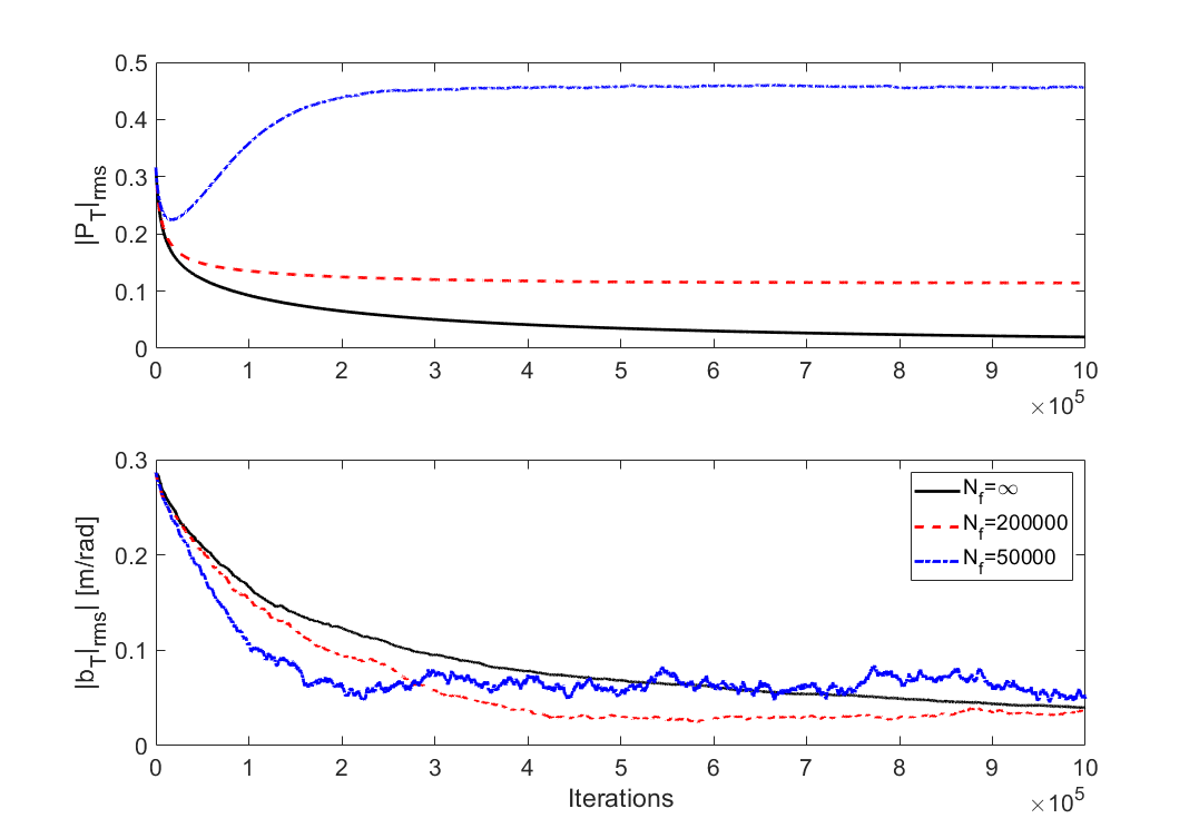
Figure 1: $|P_{T}|_{rms}$ (top) and $|b_{T}|_{rms}$ (bottom) as a function of the iterations for $N_{f}=\infty$ (solid black), $N_{f}=200\,000$ (dashed red), and $N_{f}=50\,000$ (dot dashed blue).

In order to assess the performance of our algorithm we introduce the estimation error $b_{T}=\hat{B}_{T}-B$ as the difference between estimate $\hat{B}_{T}$ and the “real” response matrix $B$ (or $\hat{B}$). The rms value of all its matrix elements $|b_{T}|_{rms}$ can be calculated from

$$|b_{T}|_{rms}=\sqrt{\frac{\mathop{\mathrm{Trace}}\left((\hat{B}_{T}-B)^{\top}(\hat{B}_{T}-B)\right)}{nm}}\ .$$ (8)

In the same fashion, we introduce $|P_{T}|_{rms}=\sqrt{\mathop{\mathrm{Trace}}\left(P_{T}^{\top}P_{T}\right)/m^{2}}$.

In a first simulation, we initialize $\hat{B}$ with the “ideal” matrix from the computer model, while we use the real matrix $B$ to model the response of the “real” system with equation 1. The upper panel in Figure 1 shows $|P_{T}|_{rms}$ for one million iterations and the lower panel shows $|b_{T}|_{rms}$. Each panel shows curves for three values of the forgetting parameter $N_{f}$. The black curves correspond to $N_{f}=\infty$ or $\alpha=1$, the case already covered in [1]. The red dashed curves correspond to $N_{f}=200\,000$ and the blue dot-dashed curves to $N_{f}=50\,000$. From the lower panel we observe that decreasing values of $N_{f}$ indeed cause $|b_{T}|_{rms}$ to decrease more quickly, albeit at the expense of an deteriorated asymptotic behavior. The read and blue curves no longer approach zero, as the black one was shown to do in [1]. This observation is consistent with the evolution of $|P_{T}|_{rms}$ shown in the upper panel. Instead of decreasing to zero, as the black curve does, the read and blue curves asymptotically approach finite limiting values. Considering that $P_{T}$ is the empirical covariance matrix that describes the error bars of the $\hat{B}_{T}$ we cannot expect them to approach $B$ arbitrarily close, as they do with $N_{f}=\infty$.

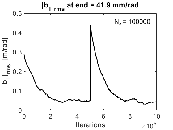
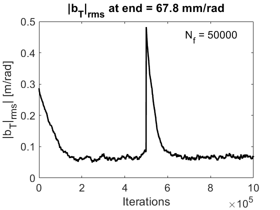
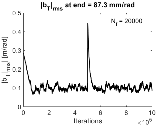
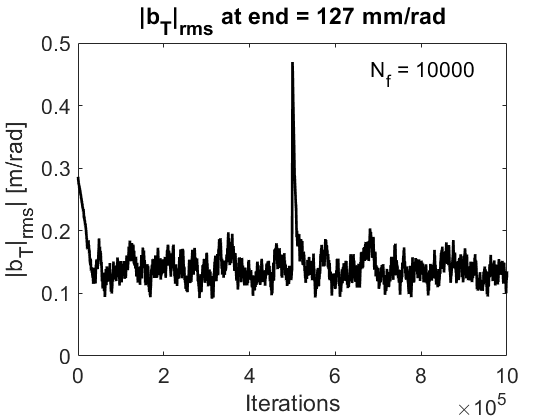
Figure 2: $|b_{T}|_{rms}$ for the four values of $N_{f}$ indicated in the top right corner of the respective plots. After 500 000 iterations the “real” system matrix $B$ is replaced by $\bar{B}$ which causes the spike in the middle of the plots.

Figure 2 shows $|b_{T}|_{rms}$ for one million iterations for six values of $N_{f}$ where, after 500 000 iterations we replace the “real” response matrix $B$ by $\bar{B}$, which is derived from a lattice with one quadrupole value changed by 5 %, as mentioned before. At the same time, we also replace $B$ by $\bar{B}$ when calculating $|b_{T}|_{rms}$, because after the new optics is in place, we expect the algorithm to converge towards $\bar{B}$, rather than $B$. The values of $N_{f}$ are indicated on the top left corner of the six plots. We observe that the algorithm in all cases uses the first half of the plot to approach $B$, already seen in Figure 1. But after the new optics is in place after 500 000 iterations, the best current approximation $\hat{B}_{T}$ differs significantly from new reference $\bar{B}$, which causes the spike in the middle part of all the plots. Forgetting the old configuration and approaching the new reference happens on the time scale given by $N_{f}$. Smaller values lead to a faster approach. Again, at the expense of a faster approach being paid for by an elevated asymptotic level, which we note in the title bar of each plot to vary from around 40 mm/rad for $N_{f}=100\,000$ to more than 120 mm/rad for $N_{f}=10\,000$.

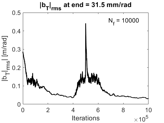
Figure 3: $|b_{T}|_{rms}$ for one million iterations while the “real” system matrix $B$ is replaced by $\bar{B}$ after $5\times 10^{5}$ iterations. For the first $10^{5}$ iterations we use $N_{f}=10\,000$, then use $N_{f}=200\,000$ between $10^{5}$ and $4\times 10^{5}$ iterations, where we again set $N_{f}=10\,000$ while the change of the system matrix occurs. After $6\times 10^{5}$ iterations we set $N_{f}=200\,000$.

In order to remedy the deteriorated asymptotic level we explored whether it is possible to temporarily adjust $N_{f}$ to allow the system to quickly react to anticipated changes in the lattice, for example, to accommodate an undulator gap to be closed. Figure 3 shows the configuration leading to the bottom right plot in Figure 2 with $N_{f}=10\,000$, only here temporarily increase $N_{f}$ to 200 000 between iteration 100 000 and 400 000 and again after iteration 600 000. We clearly see that the approximation gets better during the windows with $N_{f}=200\,000$. Once $N_{f}$ is decreased to 10 000 less information is available and the approximation gets worse, even before the change that causes the spike. But the system is much more agile to react and quickly adapts to the new system, albeit with bad precision until the larger values of $N_{f}$ after iteration 600 000 improves the estimate significantly.

Based on the discussion in this section, we suggest to adapt $N_{f}$, and thereby $\alpha$ to the anticipated running mode of the accelerator. If there is along period of tranquility, a large value is beneficial, only to be changed once more activity, for example, tune corrections or changes of undulator gaps are imminent.

In the next section we will theoretically analyze the time-dependent behavior of the system.

4 Convergence

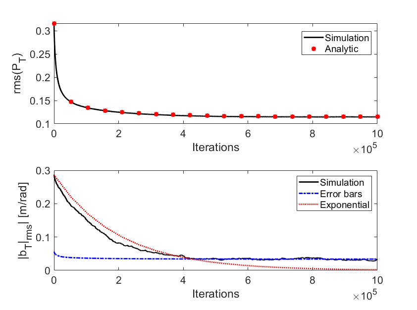
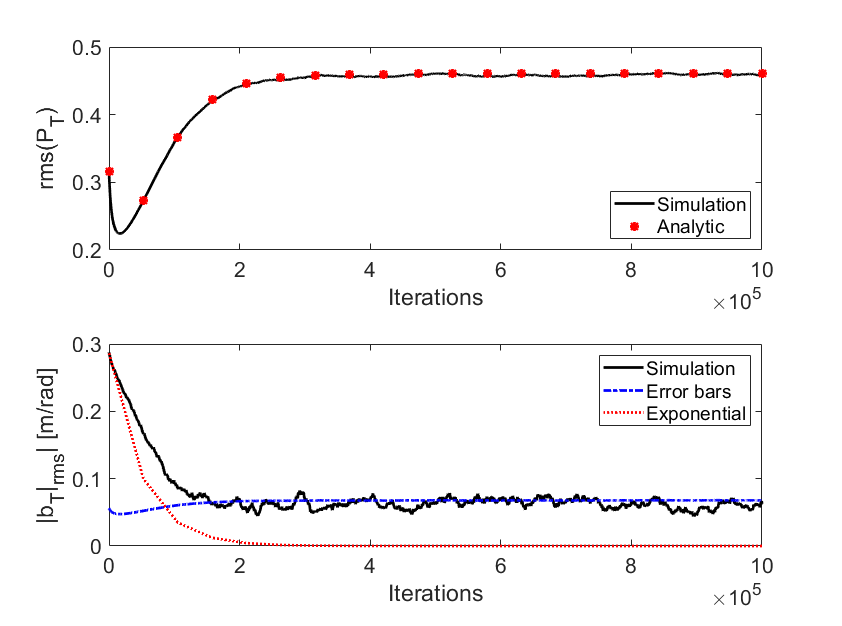
Figure 4: Simulations for $|P_{T}|_{rms}$ (top) and $|b_{T}|_{rms}$ (bottom) as well as analytic results as a function of the iterations for $N_{f}=2\times 10^{5}$ (left) and $N_{f}=5\times 10^{4}$ (right). Note how $|b_{T}|_{rms}$ initially follows and exponential form until it becomes comparable to the noise floor, indicated by the blue dot-dashed line.

Equations 6 and 7 describe the time dependence and thus also the convergence of the response matrix towards the “real” one. We first consider Equation 6, because it only depends on the most recent steerer excitation through $\ket{u_{T}}\bra{u_{T}}$, where $\ket{u_{T}}=-K\ket{x_{T}}$. Orbit correction systems are always configured such that the correction matrix $K$ is closely related to the inverse of the response matrix $B$, such that the largest eigenvalue of $1-BK$ is small. By virtue of $\ket{x_{T}}=(1-BK)\ket{x_{T-1}}+\ket{w_{T-1}}$ this implies that the most recent position $\ket{x_{T}}$ holds no or very little memory of all previous position and is dominated by noise $\ket{w_{T-1}}$. As a consequence we find $Q=\mathbf{E}\left\{\ket{u_{T}}\bra{u_{T}}\right\}\approx\sigma_{w}^{2}KK^{\top}$ is a constant matrix. See [1] for a more detailed discussion and how to include small additional variations of the steerers—so-called dithering—in the analysis.

We now insert this averaged matrix into Equation 6 and find

$$\hat{P}_{T+1}=\frac{1}{\alpha}\left[\hat{P}_{T}-\frac{\hat{P}_{T}Q\hat{P}_{T}}{\alpha+\mathop{\mathrm{Trace}}(Q\hat{P}_{T})}\right]\ ,$$ (9)

where we rewrite the expectation value in the denominator as a trace. We placed a caret over $P_{T}$ to distinguish it from the solution of Equation 6. In order to solve this system we now neglect the denominator, which is close to unity and we are left with $\hat{P}_{T+1}=(\hat{P}_{T}-\hat{P}_{T}Q\hat{P}_{T})/\alpha$ and by subtracting $\hat{P}_{T}$ on both sides we obtain $d\hat{P}_{T}/dT=\hat{P}_{T+1}-\hat{P}_{T}=(\hat{P}_{T}-\alpha\hat{P}_{t}-\hat{P}_{T}Q\hat{P}_{T})/\alpha$. Here we also introduced the difference between $\hat{P}_{T}$ in two times steps as a differential. We observe that the matrix $Q$ is by construction symmetric and we can therefore diagonalize it, which leads to $Q=ODO^{\top}$ with $D=\mathop{\mathrm{diag}}(\lambda_{1},\dots,\lambda_{m})$ and an orthogonal matrix $O$. The starting matrix $\hat{P}_{0}$ is the unit matrix and always diagonal. Therefore Equation 9 can be written as $m$ independent equations for each of the diagonal elements $p_{j,T}$ of $\hat{P}_{T}$. The differential equation for $\hat{P}_{T}$ thus defines the corresponding one for each of the modes with its particular eigenvalue $\lambda_{j}$

$$\frac{dp_{j,T}}{dT}=\left(\frac{1-\alpha}{\alpha}\right)p_{j,T}-\left(\frac{\lambda_{j}}{\alpha}\right)p_{j,T}^{2}\ ,$$ (10)

which has the solution

$$p_{j,T}=\frac{\beta}{\lambda_{j}/\alpha+(\beta/x_{0}-\lambda_{j}/\alpha)e^{-\beta T}}$$ (11)

with the abbreviation $\beta=(1-\alpha)/\alpha=1/(N_{f}-1)$. We clearly see that asymptotically $p_{T}$ approaches the finite limit $p_{j,\infty}=\alpha\beta/\lambda_{j}=1/(N_{f}\lambda_{j})$. Considering that the error bars of reconstructed response are given in terms of $P_{T}$ we can expect that increasing $N_{f}$ improves the approximation. Note that, apart from $N_{f}$, only the eigenvalues $\lambda_{j}$ of $Q=\sigma_{w}^{2}KK^{\top}$ enter. In particular, the asymptotic values are therefore inversely proportional to $\sigma_{w}$; the algorithm works better with noisy monitors, because it “learns from noise.” From the $p_{j,T}$ we can reconstruct $\hat{P}_{T}$ from

$$\hat{P}_{t}=O\mathop{\mathrm{diag}}(p_{1,T},\dots,p_{m,T})O^{\top}$$ (12)

from which we derive $|\hat{P}_{T}|_{rms}$ in the same was as for $|P_{T}|_{rms}$ that comes from the numerical simulation. The upper panels in Figure 4 show them for $N_{f}=2\times 10^{5}$ on the left and $N_{f}=5\times 10^{4}$ on the right. The agreement between simulation and Equation 12 in both cases is very good. Also the approach to finite asymptotic values is clearly visible.

Substituting $\ket{x_{T+2}}-\ket{x_{T+1}}=B\ket{u_{T+1}}$ in Equation 7 allows us to analyze the convergence of $\hat{B}_{T}$ towards $B$ from

$$\left(\hat{B}_{T+1}-B\right)=\left(\hat{B}_{T}-B\right)-\left(\hat{B}_{T}-B\right)\frac{\ket{u_{T+1}}\bra{u_{T+1}}P_{T}}{\alpha+\braket{u_{T+1}}{P_{T}}{u_{T+1}}}\ .$$ (13)

We now introduce $\hat{b}_{T}=\hat{B}_{T}-B$ to simplify writing and omit the denominator with the trace, as before. Moreover, we replace $P_{T}$ by its approximation $\hat{P}_{T}$ and replace $\ket{u_{T+1}}\bra{u_{T+1}}$ by its expectation value $Q$, which brings us to $\hat{b}_{T+1}=\hat{b}_{T}(1-Q\hat{P}_{T})$ and by turning the difference equation into a differential equation with $\hat{b}_{T+1}-\hat{b}_{T}\approx d\hat{b}_{T}/dT$ to $d\hat{b}_{T}/dT=-\hat{b}_{T}Q\hat{P}_{T}$. Despite $\hat{b}_{T}$ not being simultaneously diagonal with $\hat{P}_{T}$ and $Q$, we make the daring assumption that there are corresponding modes with eigenvalues $\kappa_{j,T}$, such that we can write

$$\frac{d\kappa_{j,T}}{\kappa_{j,T}}=-\lambda_{j}p_{j,T}dT=-\frac{\lambda_{j}\beta dT}{\lambda_{j}/\alpha+(\beta/p_{0}-\lambda_{j}/\alpha)e^{-\beta T}}\ ,$$ (14)

where we substituted $p_{j,T}$ from Equation 11. Integrating both sides, where we note that the integral on the right-hand side is elementary, we find

$$\log\left(\frac{\kappa_{j,T}}{\kappa_{j,0}}\right)=-\lambda_{j}\beta\left[\frac{\alpha T}{\lambda_{j}}+\frac{\alpha}{\beta\lambda_{j}}\log\left(\frac{\lambda_{j}}{\alpha}+\left(\frac{\beta}{p_{0}}-\frac{\lambda_{j}}{\alpha}\right)e^{-\beta T}\right)\right]\approx-\alpha\beta T$$ (15)

where we only kept the term linear in $T$ as the leading contribution. Replacing $\alpha\beta=1/N_{f}$ we see that the time scale on which the difference between $\hat{B}_{T}$ and the real response matrix $B$ vanishes is given by $e^{-T/N_{f}}$, at least in the dominant order. Since this applies to all modes $\kappa_{j}$ we feel that the daring assumption is acceptable.

On the bottom panels in Figure 4 we show the evolution of $|b_{T}|_{rms}$ coming from a simulation as black lines and $|b_{0}|_{rms}e^{-T/N_{f}}$ as the dot-dashed red line which shows a reasonable agreement. We also observe that the exponential reduction only works during the initial phase until $|b_{T}|_{rms}$ becomes comparable to the error bars that are proportional to the magnitude of the matrix elements of the empirical covariance matrix $|P_{T}|_{rms}$. We therefore also show the $\sqrt{|P_{T}|_{rms}}\sigma_{w}$ as an indication of these error bars. Once the exponential part of the convergence comes to a point where $|b_{T}|_{rms}$ becomes comparable to $\sqrt{|P_{T}|_{rms}}\sigma_{w}$ it no longer improves. The only way at this point is to increase $N_{f}$ to reduce the asymptotic values of $|P_{T}|_{rms}$ and thus lowers the noise floor, which allows $|b_{T}|_{rms}$ to decrease further. But this is just what Figure 3 shows.

In the simulations we used the same number of monitors and steerers ($n=m$), but this restriction can be overcome using the methods discussed in Section VII in [1] that we do not repeat here. Other aspects discussed there, such as delays in the system, remain equally valid.

5 Conclusions

We presented an improved version of the algorithm to noninvasively measure the orbit response matrix in storage rings. Following [10] we introduce a time horizon $N_{f}$ after which the algorithm “forgets” old information, which makes it much more agile to respond to new information, for example, due to a changed “real” response matrix. We found the time constant (in numbers of iterations) of convergence, at least initially, is given by $N_{f}$, smaller values are favorable. On the other hand, we also found that the asymptotically achievable accuracy is proportional to $1/N_{f}$, thus favoring large values of $N_{f}$.

It is however, possible, to dynamically adjust $N_{f}$ to the prevailing conditions of operation. In long periods of tranquility $N_{f}$ can be increased, only to reduce it, once changes to the accelerator configuration are expected.

We gratefully acknowledge fruitful discussions with Ingvar Ziemann, University of Pennsylvania in Philadelphia.

References

- [1] I. Ziemann, V. Ziemann, Noninvasively improving the orbit-response matrix while continuously correcting the orbit, Physical Review Accelerators and Beams 24 (2021) 072804
- [2] M. Minty, F. Zimmermann, Measurement and Control of Charged Particle Beams, Springer, Heidelberg, 2003.
- [3] X. Huang, Beam-based correction and optimization for accelerators, CRC press, Boca Raton, 2020.
- [4] J. Corbett et al., A Fast Model Calibration Procedure for Storage Rings, Proceedings of the Particle Accelerator Conference PAC93, Washington, 1993, p. 108.
- [5] J. Safranek, Experimental determination of storage ring optics using orbit response measurements, Nuclear Instruments and Methods A 388 (1997) 27.
- [6] G. Goodwin, R. Payne, Dynamic System Identification, Academic Press, London, 1977.
- [7] L. Ljung, System Identification; theory for the user, 2nd ed., Prentice Hall, New Jersey, 1999.
- [8] V. Ziemann, Regression Models and Hypothesis Testing. In: Physics and Finance. Undergraduate Lecture Notes in Physics. Springer, Cham. https://doi.org/10.1007/978-3-030-63643-2_7.
- [9] W. Press et al., Numerical Recipes, 2nd ed., Cambridge University Press, Cambridge, 1992.
- [10] Section 7.3 in [6].