Investigating Topological Order using Recurrent Neural Networks

Abstract

Recurrent neural networks (RNNs), originally developed for natural language processing, hold great promise for accurately describing strongly correlated quantum many-body systems. Here, we employ two-dimensional (2D) RNNs to investigate two prototypical quantum many-body Hamiltonians exhibiting topological order. Specifically, we demonstrate that RNN wave functions can effectively capture the topological order of the toric code and a Bose-Hubbard spin liquid on the kagome lattice by estimating their topological entanglement entropies. We also find that RNNs favor coherent superpositions of minimally-entangled states over minimally-entangled states themselves. Overall, our findings demonstrate that RNN wave functions constitute a powerful tool to study phases of matter beyond Landau’s symmetry-breaking paradigm.

I Introduction

Landau symmetry breaking theory provides a fundamental description for a wide range of phases of matter and their phase transitions through the use of local order parameters Sachdev (2011). Despite the fact that a great deal of our theoretical and experimental investigations of interacting quantum many-body systems have been developed with the aim of studying local order parameters, it is well-known that the most intriguing strongly correlated phases of matter may not be easily characterized through these observables. Instead, several states of matter seen in modern theoretical and experimental studies are defined globally through the phases’ topological properties Wen (2013); Semeghini et al. (2021); Satzinger et al. (2021). Topological order, in particular, refers to a type of order characterized by the emergence of quasi-particle anyonic excitations, topological invariants, and long-range entanglement, which typically do not appear in traditional forms of order. As a result of these properties, topologically ordered phases have been suggested as an important building block for the development of a protected qubit resistant to perturbations and errors Dennis et al. (2002); Kitaev (2006); Kitaev and Laumann (2009). Interestingly, such qubits have been devised recently at the experimental level Krinner et al. (2022); Sivak et al. (2023); Acharya et al. (2023).

While most manifestations of topological order are dynamical in nature—e.g. anyon statistics, ground state degeneracy, and edge excitations Levin and Wen (2006)–topological order can also be characterized directly in terms of the ground state wave function and its entanglement. In particular, a probe for topological order is the topological entanglement entropy (TEE) Kitaev and Preskill (2006); Levin and Wen (2006), which offers a characterization of the global entanglement pattern of topological ground states not present in conventionally ordered systems. Notably, the TEE is readily accessible for large classes of topological orders Levin and Wen (2006); Hamma et al. (2005a), in numerical simulations based on quantum Monte Carlo (QMC) Isakov et al. (2011); Wildeboer et al. (2017); Zhao et al. (2022) and density matrix renormalization group (DMRG) Jiang et al. (2012); Jiang and Balents (2013), as well as in experimental realizations of topological order based on gate-based quantum computers Satzinger et al. (2021). Machine learning (ML) techniques offer an alternative approach study quantum many-body systems and have proved useful for a wide array of tasks including the classification of phases of matter Carrasquilla and Melko (2017); Broecker et al. (2017); Ch’ng et al. (2017); Miles et al. (2021), quantum state tomography Torlai et al. (2018); Carrasquilla et al. (2019), finding ground states of quantum systems Androsiuk et al. (1993); LAG (1997); Carleo and Troyer (2017); Cai and Liu (2018); Luo and Clark (2019); Pfau et al. (2020); Hermann et al. (2020); Choo et al. (2020); Hibat-Allah et al. (2020); Roth (2020), studying open quantum systems Vicentini et al. (2019); Luo et al. (2022), and simulating quantum circuits Jónsson et al. (2018); Medvidović and Carleo (2021); Carrasquilla et al. (2021), among many others Dunjko and Briegel (2018); Carleo et al. (2019); Carrasquilla (2020); Dawid et al. (2022). In particular, neural networks representations of quantum many-body states have been shown to be able of expressing topological order using, e.g., restricted Boltzmann machines Deng et al. (2017); Glasser et al. (2018); Chen et al. (2018); Lu et al. (2019), convolutional neural networks Carrasquilla and Melko (2017) and autoregressive neural networks Luo et al. (2021). Here we use recurrent neural networks (RNN) Hochreiter and Schmidhuber (1997); Graves (2012); Lipton et al. (2015) as an ansatz wave function Hibat-Allah et al. (2020); Roth (2020) to investigate topological order in two dimensions (2D) through the estimation of the TEE. We focus on two model Hamiltonians exhibiting topological order, namely Kitaev’s toric code Kitaev (2006); Kitaev and Laumann (2009) and a Bose-Hubbard model on the kagome lattice previously shown to host a gapped quantum spin liquid with non-trivial emergent $\mathbb{Z}_{2}$ gauge symmetry Isakov et al. (2006, 2011); Zhao et al. (2022). In our study, we use Kitaev-Preskill constructions Kitaev and Preskill (2006), and finite size-scaling analysis of the entanglement entropy to extract the TEE. We find convincing evidence that RNNs are capable of expressing ground states of Hamiltonians displaying topological order. We also find evidence that the RNN wave function is naturally biased toward finding superpositions of minimally entangled states (MESs), as reflected in the calculations of entanglement entropy and Wilson loop operators for the toric code. Overall, our results indicate that RNNs can represent phases of matter beyond the conventional Landau symmetry-breaking paradigm.

II 2D RNN

Our main aim is to study topological properties of Hamiltonians using an RNN wave function ansatz. Since the quantum systems we study are stoquastic Bravyi (2015), we consider an ansatz with positive amplitudes to model the ground state wave function Hibat-Allah et al. (2020). Complex extensions of RNN wave functions for non-stoquastic Hamiltonians have been explored in Refs. Hibat-Allah et al. (2020); Roth (2020). To model a positive RNN wave function, we write our ansatz in the computational basis as:

$$\Psi_{\bm{\theta}}(\bm{\sigma})=\sqrt{p_{\bm{\theta}}(\bm{\sigma})},$$

where $\bm{\theta}$ denotes the variational parameters of the ansatz $\ket{\Psi_{\bm{\theta}}}$, and $\bm{\sigma}=(\sigma_{1},\sigma_{2},\ldots,\sigma_{N})$ is a basis state configuration. A key characteristic of the RNN wave function is its ability to estimate observables with uncorrelated samples through autoregressive sampling Hibat-Allah et al. (2020); Ferris and Vidal (2012). This is achieved by parametrizing the joint probability $p_{\bm{\theta}}(\bm{\sigma})$ with its conditionals $p_{\bm{\theta}}(\sigma_{i}|\sigma_{<i})$, through the probability chain rule

$$p_{\bm{\theta}}(\bm{\sigma})=p_{\bm{\theta}}(\sigma_{1})p_{\bm{\theta}}(\sigma_{2}|\sigma_{1})\cdots p_{\bm{\theta}}(\sigma_{N}|\sigma_{N-1},\dots,\sigma_{2},\sigma_{1}).$$

The conditionals are given by

$$p_{\bm{\theta}}(\sigma_{i}|\sigma_{<i})=\bm{y}_{i}\cdot\bm{\sigma}_{i},$$

where $\bm{y}_{i}=\text{Softmax}(U\bm{h}_{i}+\bm{c})$ and ‘$\cdot$’ is the dot product operation. The hidden state $\bm{h}_{i}$ is calculated recursively as Lipton et al. (2015)

$$\bm{h}_{i}=f\!(W[\bm{\sigma}_{i-1};\bm{h}_{i-1}]+\bm{b}),$$ (1)

where the input $\bm{\sigma}_{i-1}$ is a one-hot encoding of $\sigma_{i-1}$ and the symbol $[.;.]$ corresponds to the concatenation of two vectors. Furthermore, $U,W,\bm{b}$, and $\bm{c}$ are learnable weights and biases and $f$ is an activation function. The sequential operation of the RNN is shown in Fig. 1(a), where the RNN cell, i.e., the recurrent relation in Eq. (1), is depicted as a blue square. As each of the conditionals $p_{\bm{\theta}}(\sigma_{i}|\sigma_{<i})$ Hibat-Allah et al. (2020) is normalized, the distribution $p_{\bm{\theta}}$, and thus the quantum state $|\Psi_{\bm{\theta}}\rangle$, are normalized. Notably, by virtue of the sequential structure built into the RNN ansatz, it is possible to obtain exact samples from $p_{\bm{\theta}}$ by sampling the conditionals $p_{\bm{\theta}}(\sigma_{i}|\sigma_{<i})$ sequentially as illustrated in Fig. 1(b). The sampling scheme is parallelizable and can produce fully uncorrelated samples distributed according to $p_{\bm{\theta}}$ without the use of potentially slow Markov chains Hibat-Allah et al. (2020); Roth (2020).

As our aim is to study 2D quantum systems with periodic boundary conditions, we use 2D RNNs Graves et al. (2007); Hibat-Allah et al. (2020), through the modification of the 1D relation in Eq. (1) to a recursion that encodes the 2D geometry of the lattice, i.e.,

$$\bm{h}_{i,j} =f\!\Big{(}W[\bm{\sigma}_{i-(-1)^{j},j};\bm{\sigma}_{i,j-1};\bm{h}_{i-(-1)^{j},j};\bm{h}_{i,j-1}]+\bm{b}\Big{)}.$$ (2)

Here $\bm{h}_{i,j}$ is a hidden state with two indices for each site in the 2D lattice, which is computed based on the inputs and the hidden states of the nearest neighboring sites. Note that the $x$-index of the horizontal neighboring site follows the zigzag sampling path illustrated by the red dashed arrows in Fig. 1(c). This sampling path was motivated in Ref. Hibat-Allah et al. (2020), which allows us to circumvent the use of non-local recurrent connections in our 2D RNN as opposed to other sampling paths. Other alternative orderings are discussed in Ref. Jain et al. (2020). Since $\bm{h}_{i,j}$ contains information about of the history of generated variables $\sigma_{i,j}$, it can be used to compute the conditionals

$$p_{\bm{\theta}}(\sigma_{i,j}|\sigma_{<i,j})=\text{Softmax}(U\bm{h}_{i,j}+\bm{c})\cdot\bm{\sigma}_{i,j}.$$ (3)

It is worth noting that at the boundaries of the 2D lattice, we use additional inputs to the 2D recursion relation as follows:

$$\bm{h}_{i,j} =f\!\Big{(}W^{\prime}[\bm{\sigma}_{i-(-1)^{j},j};\bm{\sigma}_{i,j-1};\bm{\sigma}_{i+(-1)^{j},j};\bm{\sigma}_{i,j+1};$$

$$\bm{h}_{i-(-1)^{j},j};\bm{h}_{i,j-1};\bm{h}_{i+(-1)^{j},j};\bm{h}_{i,j+1}]+\bm{b}^{\prime}\Big{)}.$$ (4)

For consistency, $W^{\prime}$ and $\bm{b}^{\prime}$ are extensions of the weights $W$ and $\bm{b}$ in Eq. (2). Additionally, $L_{x},L_{y}$ are respectively the width and the length of the 2D lattice. In our study, we choose $L_{x}=L_{y}=L$. The additional variables $\bm{\sigma}_{i+(-1)^{j},j}$, $\bm{\sigma}_{i,j+1}$ and hidden states $\bm{h}_{i+(-1)^{j},j}$, $\bm{h}_{i,j+1}$ allow modeling systems with periodic boundary conditions such that the ansatz accounts for the correlations between physical degrees of freedom across the boundaries as suggested in Ref. Luo et al. (2021). For more clarity, periodic boundary conditions on the indices of the hidden states and the inputs are assumed. Furthermore, we note that during the process of autoregressive sampling, if either of the input vectors, in Eq. (4), have not been encountered yet, we initialize them to a null vector so we preserve the autoregressive nature of the RNN wave function, as illustrated in Fig. 1(b). Furthermore, Fig. 1(c) illustrates the autoregressive sampling path in 2D and how information is being transferred among RNN cells. Importantly, we use an advanced version of 2D RNNs which incorporates a gating mechanism to mitigate the vanishing gradient problem Hibat-Allah et al. (2020); Casert et al. (2021); Luo et al. (2021); Hibat-Allah et al. . Additional details can be found in App. A. We also note that implementing lattice symmetries in our RNN ansatz can be done to improve the variational accuracy as shown in Refs. Hibat-Allah et al. (2020, ), however, we do not pursue this direction in our study.

Finally, to highlight the advantages of our RNN approach, we note that the training complexity of one gradient descent step of the 2D RNN wave function is quadratic in the size of hidden states denoted as $d_{h}$. The latter is very inexpensive compared to projected-entangled pair-states (PEPS), which is $\#$P to contract in general Haferkamp et al. (2020) and can be approximately contracted with a scaling $\mathcal{O}(\chi^{2}\tilde{D}^{6})$ (where $\tilde{D}$ the PEPS bond dimension and $\chi$ is the bond dimension of the intermediate matrix product state (MPS) Vanderstraeten et al. (2016). It is also worth noting that RNNs have the weight-sharing property which allows the extrapolation of small system size calculations to larger system sizes Roth (2020); Hibat-Allah et al. as illustrated in Sec. III.2. We would also like to point out that the sampling and the inference cost of the RNN is linear in the system size which favors RNNs compared to other autoregressive models in terms of computational cost Hibat-Allah et al. (2020); Luo et al. (2021).

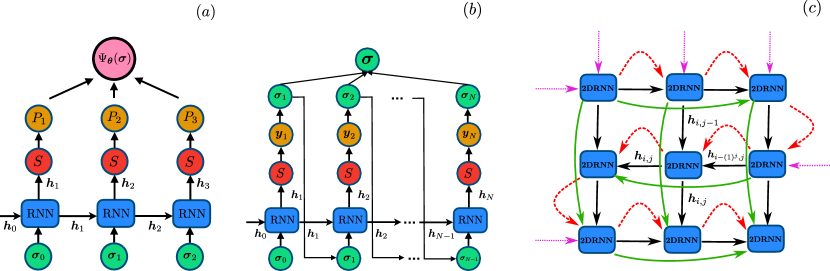
Figure 1: (a) An illustration of the positive RNN wave function. Each RNN cell (blue squares) receives an input $\bm{\sigma}_{n-1}$ and a hidden state $\bm{h}_{n-1}$ and outputs a new hidden state $\bm{h}_{n}$. The latter is fed to a Softmax layer (denoted by S, red circle) that outputs a conditional probability $P_{i}$ (orange circle). The conditional probabilities are multiplied after taking a square root to obtain the wave function $\Psi_{\bm{\theta}}(\bm{\sigma})$ (pink circle). (b) Illustration of the sampling scheme for an RNN wave function. After obtaining the probability vector $\bm{y}_{i}$ from the Softmax layer (S) at step $i$, we sample it to produce $\bm{\sigma}_{i}$ which is fed again to the RNN with the hidden state $\bm{h}_{i}$ to produce the next configuration $\bm{\sigma}_{i+1}$.(c) A 2D RNN with periodic boundary conditions. A bulk RNN cell receives two hidden states $\bm{h}_{i,j-1}$ and $\bm{h}_{i-(-1)^{j},j}$, as well as two input vectors $\bm{\sigma}_{i,j-1}$ and $\bm{\sigma}_{i-(-1)^{j},j}$ (not shown) illustrated by the black solid arrows. To handle periodic boundary conditions, RNN cells at the boundary receive an additional $\bm{h}_{i,j+1}$ and $\bm{h}_{i+(-1)^{j},j}$, as well as two input vectors $\bm{\sigma}_{i,j+1}$ and $\bm{\sigma}_{i+(-1)^{j},j}$ (not shown) illustrated by green solid arrows. The sampling path is illustrated with curved dashed red arrows. The initial memory states and the initial inputs are taken as null vectors and are fed to the 2DRNN cells as indicated by the pink dashed arrows.

II.1 Supplementing RNNs optimization with annealing

To train the parameters of the RNN, we minimize the energy expectation value $E_{\bm{\theta}}=\bra{\Psi_{\bm{\theta}}}\hat{H}\ket{\Psi_{\bm{\theta}}}$ using Variational Monte Carlo (VMC) Becca and Sorella (2017), where $\hat{H}$ is a Hamiltonian of interest. In the presence of local minima in the optimization landscape of $E_{\bm{\theta}}$, the VMC optimization may get stuck in a poor local optimum Hibat-Allah et al. (2021); Bukov et al. (2021). To ameliorate this limitation, we supplement the VMC scheme with a pseudo-entropy whose objective is to help the optimization escape local minima Roth (2020); Hibat-Allah et al. (2021, ); Roth et al. (2022); Khandoker et al. (2023). The new objective function is defined as

$$F_{\bm{\theta}}(n)=E_{\bm{\theta}}-T(n)S_{\rm classical}(p_{\bm{\theta}}),$$ (5)

where $F_{\bm{\theta}}$ is a variational pseudo free energy. The Shannon entropy $S_{\rm classical}$ of $p_{\bm{\theta}}\left(\bm{\sigma}\right)$ is given by

$$S_{\rm classical}(p_{\bm{\theta}})=-\sum_{\bm{\sigma}}p_{\bm{\theta}}(\bm{\sigma})\ln\left(p_{\bm{\theta}}(\bm{\sigma})\right),$$ (6)

where the sum goes over all possible configurations $\{\bm{\sigma}\}$ in the computational basis. The pseudo-entropy $S_{\rm classical}$ and its gradients are evaluated by sampling the RNN wave function. Furthermore, $T(n)$ is a pseudo-temperature that is annealed from some initial value $T_{0}$ to zero as follows: $T(n)=T_{0}(1-n/N_{\rm annealing})$ where $n\in[0,N_{\rm annealing}]$ and $N_{\rm annealing}$ is the total number of annealing steps. This scheme is inspired by the regularized variational quantum annealing scheme in Refs. Roth (2020); Hibat-Allah et al. (2021, ). More details about our training scheme are given in App. B. We also provide the hyperparameters in App. C.

II.2 Topological entanglement entropy

A powerful tool to probe topologically ordered states of matter is through the TEE Hamma et al. (2005a, b); Levin and Wen (2006); Kitaev and Preskill (2006); Flammia et al. (2009); Zhang et al. (2012); Isakov et al. (2011); Wildeboer et al. (2017); Kim et al. (2023). The TEE can be extracted by computing the entanglement entropy of a spatial bipartition of the system into $A$ and $B$, which together comprise the full system. For many phases of 2D matter, the Renyi-$n$ entropy $S_{n}(A)\equiv\frac{1}{1-n}\ln(\text{Tr}(\rho^{n}_{A}))$ satisfies the area law $S_{n}(A)=aL_{A}-\gamma+\mathcal{O}(L^{-1})$. Here $L_{A}$ is the size of the boundary between $A$ and $B$, $\rho_{A}=\text{Tr}_{B}|\Psi\rangle\langle\Psi|$ is the reduced density matrix of subsystem $A$, $|\Psi\rangle$ is the state of the system, and $\gamma$ is the TEE. The latter detects non-local correlations in the ground state wave function and plays the role of an order parameter for topological phases similar to the notion of a local order parameter in phases displaying long-range order. Interestingly, a measure of specific non-zero values of $\gamma$ can be a clear sign of the existence of a topological order in a system of interest. Additionally, since the TEE is shown to be independent of the choice of Renyi index $n$ for a contractible region $A$ Flammia et al. (2009), we can use the swap trick Hastings et al. (2010) with our RNN wave function ansatz Hibat-Allah et al. (2020); Wang and Davis (2020) to calculate the second Renyi entropy $S_{2}$ and extract the TEE $\gamma$.

To access the TEE $\gamma$, we can approximate the ground state of the system using an RNN wave function ansatz, i.e. $|\Psi_{\bm{\theta}}\rangle\approx|\Psi\rangle$ for different system sizes followed by a finite-size scaling analysis of the second Renyi entropy. We can also make use of a TEE construction, e.g., the Kitaev-Preskill construction Kitaev and Preskill (2006).

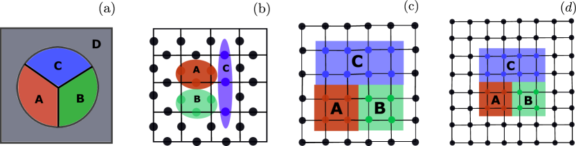
Figure 2: Panel (a): a sketch of the parts $A$, $B$, and $C$ that we use for Kitaev-Preskill construction to compute the TEE in a system of interest. Panels (b-d): an illustration of the subregions $A,B,C$ chosen for the Kitaev-Preskill constructions. (b) For the 2D toric code, each subregion has $3$ spins. We also do the same for the lattice lengths $L=6,8,10$ in Fig. 4(b). For the hard-core Bose-Hubbard model on the Kagome lattice, we target two different system sizes. Panel (c) shows the construction for $L=6$ and panel (d) provides the construction for $L=8$. In panels (c) and (d), each site corresponds to a block of three bosons.

The Kitaev-Preskill construction prescribes dividing the system into four subregions $A$, $B$, $C$, and $D$ as illustrated in Fig. 2. The TEE can be then obtained by computing

$$\gamma =-S_{2}(A)-S_{2}(B)-S_{2}(C)+S_{2}(AB)$$

$$+S_{2}(AC)+S_{2}(BC)-S_{2}(ABC),$$

where $S_{2}(A)$ is the second Renyi entropy of the subsystem $A$, and $AB$ is the union of $A$ and $B$ and similarly for the other terms. Finite-size effects on $\gamma$ can be alleviated by increasing the size of the subregions $A,B$ and $C$ Kitaev and Preskill (2006); Furukawa and Misguich (2007). Here we have fixed the size of the interior subregions $A$, $B$, $C$ to limit the error bars in our calculations. Finally, we highlight the ability of the RNN wave function to study systems with fully periodic boundary conditions as a strategy to mitigate boundary effects, as opposed to cylinders used in DMRG Stoudenmire and White (2012); Gong et al. (2014), which may potentially introduce edge effects that can affect the values of the TEE Samajdar et al. (2021).

III Results

III.1 The toric code

We now focus our attention on the toric code Hamiltonian which is the simplest model that hosts a $Z_{2}$ topological order Kitaev (2006); Hamma et al. (2005b) and has a non-zero TEE equal to $\gamma=\ln(2)$. The Hamiltonian is defined in terms of spin-$1/2$ degrees of freedom located on the edges of a square lattice (see Fig. 3(a)) and is given by

$$\hat{H}=-\sum_{p}\prod_{i\in p}\hat{\sigma}_{i}^{z}-\sum_{v}\prod_{i\in v}\hat{\sigma}_{i}^{x},$$

where $\hat{\sigma}_{i}^{x,z}$ are Pauli matrices. Additionally, the first summation is on the plaquettes and the second summation is on the vertices of the lattice Hamma et al. (2005b). Note that the lattice in Fig. 3(a) can be seen as a square lattice with a unit cell containing two spins. In our simulations, we use an $L\times L\times 2$ array of spins where $L$ is the number of plaquettes on each side of the underlying square lattice. It is possible to study the toric code with a 2D RNN defined on a primitive square lattice by merging the two spin degrees of freedom of the unit cell of the toric code into a single “patch” followed by an enlargement of the local Hilbert space dimension in the RNN from $2$ to $4$. This idea is illustrated in Fig. 3(a) and is similar in spirit to how the local Hilbert space is enlarged in DMRG to study quasi-1D systems Milsted et al. (2019). We provide additional details about the mapping in App. A.

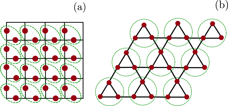
Figure 3: Mapping of 2D toric code lattice and kagome lattice to a square lattice that can be handled by a 2D RNN wave function. For the toric code lattice in panel (a), every two sites inside the dashed green ellipses are merged. For the kagome lattice in panel (c), every three sites in a unit cell enclosed by the dashed green circles are combined.

To extract the TEE from our ansatz, we variationally optimize the 2D RNN wave function targetting the ground state of this model for multiple system sizes on a square lattice with periodic boundary conditions. After the optimization, we compute the TEE using system size extrapolation and using the Kitaev-Preskill scheme provided in Sec. II.2. Here we use three spins for each subregion as illustrated in Fig. 2(b). To avoid local minima during the variational optimization, we perform an initial annealing phase as described in Sec. II.1 (see additional details in App. C).

The results shown in Fig. 4(a) suggest that our 2D RNN wave function can describe states with an area law scaling in 2D. Linearized versions of the RNN wave function have been recently shown to display an entanglement area law Wu et al. (2022). For $L=10$ (not included in the extrapolations in Fig. 4(a)), it is challenging to evaluate $S_{2}$ accurately as the expectation value of the swap operator is proportional to $\exp{(-S_{2})}$, which becomes very small and is hard to resolve accurately via sampling the RNN wave function. The improved ratio trick is an interesting alternative for enhancing the accuracy of our estimates Hastings et al. (2010); Torlai et al. (2018). The use of conditional sampling is also another possibility for enhancing the accuracy of our measurements Wang and Davis (2020).

Additionally, the extrapolation confirms the existence of a non-zero TEE whose value is close to $\gamma^{\prime}=\ln(2)$ within error bars. To further verify that our 2D RNN wave function can extract the correct TEE of the 2D toric code, we compute the TEE using the Preskill-Kitaev construction, which has contractible surfaces, and for which the TEE does not depend on the topological sector superposition Zhang et al. (2012); Wildeboer et al. (2017) (see Fig. 2(b)). The results reported in Fig. 4(b) demonstrate an excellent agreement between the TEE extracted by our RNN and the expected theoretical value for the toric code. To keep the error bars small, and since in the toric code the TEE does not depend on the subregion sizes Hamma et al. (2005b), we use fixed subregion sizes in Fig. 2(b).

Interestingly, we note that the subregion we use to compute the TEE in Fig. 4(a) is half of the torus, namely a cylinder with two disconnected boundaries . As shown in Ref. Zhang et al. (2012), the use of this non-contractible geometry means that the expected TEE becomes state-dependent and given by

$$\gamma^{\prime}=2\gamma+\ln\left(\sum_{i}\frac{p_{i}^{2}}{d_{i}^{2}}\right)$$ (7)

for the second Renyi entropy. Here $d_{i}\geq 1$ is the quantum dimension of an $i$-th quasi-particle. For the toric code, we have Abelian anyons with $d_{i}=1$ for $i=1,2,3,4$. Additionally $p_{i}=|\alpha_{i}|^{2}$ is the overlap of the computed ground state $\ket{\Psi}$ with the $i$-th MES $\ket{\Xi_{i}}$ where

$$\ket{\Psi}=\sum_{i}\alpha_{i}\ket{\Xi_{i}}.$$

The observations above and the numerical result $\gamma^{\prime}_{\text{RNN}}\approx\ln(2)$, for the non-contractible subregions in Fig. 4(a), suggest that the RNN wave functions optimized via gradient descent and annealing find a superposition of MES, as opposed to DMRG which preferentially collapses to a single MES for relatively low bond dimensions. For relatively large bond dimensions a superposition of MES can be recovered in a DMRG simulation Jiang et al. (2012); Jiang and Balents (2013).

Here we further investigate the superposition found by the RNN through the analyses of the expectation values of the average Wilson loop operators and the average ’t Hooft loop operators. First of all, we check that our RNN energy has converged to the ground state energy as shown in Tab. 1. This convergence confirms that our RNN wave function satisfies the plaquette and the vertice constraints with an excellent approximation.

Length $L$	$L=4$	$L=6$	$L=8$	$L=10$
Energy per spin	-1.99970(3)	-1.99962(2)	-1.99975(1)	-1.99986(1)

Table 1: Variational energies per site found by our RNN wave function for the 2D toric code for different lattice lengths $L$ after autoregressively sampling $10^{5}$ configurations at the end of training. We find an excellent agreement with the ground state energy per site $-2$.

Next, we define the average Wilson loop operators as

$$\hat{W}^{z}_{d}=\frac{1}{L}\left(\sum_{\mathcal{C}_{d}}\prod_{\sigma_{j}\in\mathcal{C}_{d}}\hat{\sigma}_{j}^{z}\right).$$ (8)

Here $d=h,v$ and $\mathcal{C}_{h},\mathcal{C}_{v}$ are closed non-contractible loops illustrated in Fig. 5. A set of degenerate ground states of the toric code are eigenstates of the operators $\hat{W}^{z}_{h}$, $\hat{W}^{z}_{v}$ with eigenvalues $\pm 1$. Additionally, the two eigenvalues uniquely determine the topological sector of the ground state. In this case, the topological ground states can be labeled as $\ket{\xi_{ab}}$ with $a,b=0,1$ Zhang et al. (2012); Fradkin (2013).

We can also define the average ’t Hooft loop operators on non-contractible closed loops Fradkin (2013), such that

$$\hat{W}^{x}_{d}=\frac{1}{L}\left(\sum_{\mathcal{C}_{d}}\prod_{\sigma_{j}\in\tilde{\mathcal{C}}_{d}}\hat{\sigma}_{j}^{x}\right),$$ (9)

where $d=h,v$ and $\tilde{\mathcal{C}}_{h}$, $\tilde{\mathcal{C}}_{v}$ correspond to horizontal and vertical loops as illustrated in Fig. 5. These operators satisfy the anti-commutation relations $\{\hat{W}^{z}_{h},\hat{W}^{x}_{v}\}=0$ and $\{\hat{W}^{z}_{v},\hat{W}^{x}_{h}\}=0$.

Figure 4: Entanglement properties of the 2D toric code. (a) Second Renyi entropy $S_{2}$ scaling is computed using our RNN wave function on the 2D toric code for different lengths of the boundary $L_{A}=L$, where $L$ is the system length and the total system size is given as $L\times L\times 2$. Note that our toric code embedded in a torus is divided into two equal cylinders to compute $S_{2}$. (b) TEE computed with the Kitaev-Preskill construction (see Fig. 2(b)) versus the overall system length $L$. The values found by the RNN are very close to $\ln(2)$. Error bars correspond to one standard deviation and are smaller than the symbol size.

From the optimized RNN wave function ($L=8$), we find $\langle\hat{W}^{z}_{h}\rangle=0.0009(2)$ and $\langle\hat{W}^{z}_{v}\rangle=-0.0039(2)$ which are consistent with vanishing expectation values. We also obtain $\langle\hat{W}^{x}_{h}\rangle=0.999847(5)$ and $\langle\hat{W}^{x}_{v}\rangle=0.999785(5)$ for the ’t Hooft loop operators, which are consistent with $+1$ expectation values. These results are in part due to the use of a positive RNN wave function which forces the expectation values $\langle\hat{W}^{x}_{h}\rangle$ and $\langle\hat{W}^{x}_{v}\rangle$ to strictly positive values and rules out the possibility to obtain, e.g., $\langle\hat{W}^{x}_{h}\rangle=-1$.

By expanding the optimized RNN wave function in the $\ket{\xi_{ab}}$ basis, where $a,b$ are binary variables, we obtain

$$\ket{\Psi_{\text{RNN}}}\approx\sum_{ab}c_{ab}\ket{\xi_{ab}}.$$

Here $\{\ket{\xi_{ab}}\}$ correspond to the four topological sectors and they are mutually orthogonal. $c_{ab}$ are real numbers since we use a real-valued (specifically positive) ansatz wave function. Additionally, the basis states $\ket{\xi_{ab}}$ satisfy

$$\hat{W}^{z}_{h}\ket{\xi_{ab}}=(-1)^{a}\ket{\xi_{ab}},$$

$$\hat{W}^{z}_{v}\ket{\xi_{ab}}=(-1)^{b}\ket{\xi_{ab}}.$$

From the anti-commutation relations, we can show that:

$$\hat{W}^{x}_{h}\ket{\xi_{ab}}=\ket{\xi_{a\bar{b}}},$$

$$\hat{W}^{x}_{v}\ket{\xi_{ab}}=\ket{\xi_{\bar{a}b}},$$

where $\bar{a}=1-a$ and $\bar{b}=1-b$. By plugging the last two equations in the $\hat{W}^{x}_{h}$, $\hat{W}^{x}_{v}$ expectation values of our optimized RNN wave function, we obtain:

$$2c_{00}c_{01}+2c_{10}c_{11}\approx 1,$$

$$2c_{00}c_{10}+2c_{01}c_{11}\approx 1.$$

From the normalization constraint $1=\sum_{ab}c_{ab}^{2}$, we deduce that:

$$(c_{00}-c_{01})^{2}+(c_{10}-c_{11})^{2}\approx 0,$$

$$(c_{00}-c_{10})^{2}+(c_{01}-c_{11})^{2}\approx 0.$$

As a consequence, we conclude that $c_{00}\approx c_{01}\approx c_{10}\approx c_{11}$, which means that the optimized RNN wave function is approximately a uniform superposition of the four topological ground states $\ket{\xi_{ab}}$. This observation is also consistent with vanishing expectation values of the operators $\hat{W}^{z}_{h}$, $\hat{W}^{z}_{v}$.

Furthermore, from Ref. Zhang et al. (2012) the MES of the toric code are given as follows:

$$\ket{\Xi_{1}}=\frac{1}{\sqrt{2}}\left(\ket{\xi_{00}}+\ket{\xi_{01}}\right),$$

$$\ket{\Xi_{2}}=\frac{1}{\sqrt{2}}\left(\ket{\xi_{00}}-\ket{\xi_{01}}\right),$$

$$\ket{\Xi_{3}}=\frac{1}{\sqrt{2}}\left(\ket{\xi_{10}}+\ket{\xi_{11}}\right),$$

$$\ket{\Xi_{4}}=\frac{1}{\sqrt{2}}\left(\ket{\xi_{10}}-\ket{\xi_{11}}\right).$$

Thus, our RNN wave function can be written approximately as a uniform superposition of the MESs $\ket{\Xi_{1}}$ and $\ket{\Xi_{3}}$, i.e.

$$\ket{\Psi_{\text{RNN}}}\approx\frac{1}{\sqrt{2}}\left(\ket{\Xi_{1}}+\ket{\Xi_{3}}\right).$$

In conclusion, using Eq. (7), we expect $\gamma^{\prime}=2\ln(2)+\ln\left(\frac{1}{4}+\frac{1}{4}\right)=\ln(2)$, which is consistent with our numerical observations.

We note that the exact autoregressive sampling procedure plays a key role in the ability of our RNN ansatz to sample a superposition of different topological sectors when this superposition is encoded in our ansatz. For wave functions representing the ground state of the toric code used in combination with Markov-chain Monte Carlo methods, the probability of sampling different topological sectors of the state is exponentially suppressed even if the exact wave function ansatz encodes different topological sectors. This observation can be illustrated using an exact convolutional neural network construction of the toric code ground state which contains an equal superposition of different topological sectors Carrasquilla and Melko (2017). Although in principle such representation contains all topological sectors, its form is not amenable to exact sampling and uses Markov chains so, upon sampling with local moves, the system chooses a fixed topological sector.

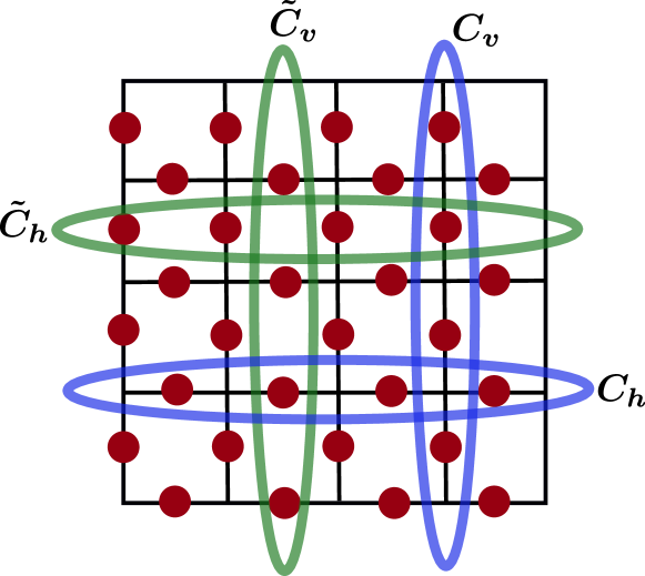
Figure 5: An illustration of the vertical and the horizontal loops used to compute the Wilson loop operators (see Eq. 8) and the ’t Hooft loop operators (see Eq. 9).

III.2 Bose-Hubbard model on kagome lattice

We now turn our attention to a hard-core Bose-Hubbard model on the kagome lattice, which has been shown to host topological order Isakov et al. (2006, 2011); Zhao et al. (2022). The Hamiltonian of this model is given by

$$\hat{H}=-t\sum_{\langle i,j\rangle}\left(b_{i}^{\dagger}b_{j}+b_{i}b_{j}^{\dagger}\right)+V\sum_{\hexagon}n_{\hexagon}^{2},$$ (10)

where $b_{i}$ ($b_{i}^{\dagger}$) is the annilihation (creation) operator. Furthermore, $t$ is the kinetic strength, $V$ is a tunable interaction strength and $n_{\hexagon}=\sum_{i\in\hexagon}(n_{i}-1/2)$. The first term corresponds to a kinetic term that favors hopping between nearest neighbors, whereas the second term promotes an occupation of three hard-core bosons in each hexagon of the kagome lattice. In our setup, we choose $V$ in units of the kinetic term strength $t$. Note that for a hard-core boson $i$, the occupation $n_{i}=b_{i}^{\dagger}b_{i}$ only takes two values $0$ or $1$.

The atom configurations of this model correspond to an $L\times L\times 3$ array of binary degrees of freedom where $L$ is the size of each side of the kagome lattice. Following an analogous approach to the toric code, we combine three sites of the unit cell of the kagome lattice as input to the 2D RNN cell, as illustrated in Fig. 3(b). This allows us to map our kagome lattice with a local Hilbert space of $2$ to a square lattice with an enlarged Hilbert space of size $2^{3}=8$.

The model is known to host a $Z_{2}$ spin-liquid phase for $V\gtrsim 7$ Isakov et al. (2011); Wang et al. (2017); Zhao et al. (2022). To confirm this finding, we estimate $\gamma$ for the system sizes $6\times 6\times 3$ and $8\times 8\times 3$. We use the Kitaev-Preskill construction Kitaev and Preskill (2006). The details of the construction of the regions $A,B$ and $C$ are provided in Figs. 2(c-d). As the Hamiltonian in Eq. 10 has a $U(1)$ symmetry associated with the conservation of bosons in the system, we impose this symmetry on our RNN wave function Hibat-Allah et al. (2020). We also supplement the VMC optimization with annealing to overcome local minima as previously done for the 2D toric code (see App. B). For the system size $8\times 8\times 3$, the RNN ansatz parameters were initialized using the optimized parameters of the system size $6\times 6\times 3$ (see details about the hyperparameters in App. C). This pre-training technique was motivated by Refs. Roth (2020); Hibat-Allah et al. ; Luo et al. (2021).

The results are provided in Fig. 6. The computed TEEs for $L=6,8$ show a saturation of $\gamma_{\rm RNN}$ for large values of the interaction strength $V$. We observe that the saturation values of $\gamma_{\rm RNN}$ are in good agreement with the expected TEE $\gamma=\ln(2)$ of a $Z_{2}$ spin-liquid Isakov et al. (2011). Additionally, the negative values of $\gamma_{\rm RNN}$ observed for $V\leq 6$ in the superfluid phase Isakov et al. (2011) may be related to the presence of Goldstone modes that manifest themselves as corrections to the area law in the entanglement entropy and can be seen as a negative contribution to the TEE Kulchytskyy et al. (2015). We note that the QMC methods are capable of obtaining a consistent value with the exact TEE for this model at $V=8$ for very large system sizes Zhao et al. (2022) using finite-size extrapolation. This observation suggests that our RNN ansatz is still limited by finite-size effects at $V=8$ (see Fig. 6) for which the TEE is not yet saturated to $\ln{2}$. Other sources of error in our calculation may be due to inaccuracies in the variational calculations and statistical errors due to the sampling. However, we note that our variational calculation is performed at zero temperature, which makes our calculations insensitive to temperature effects as opposed to QMC Isakov et al. (2011).

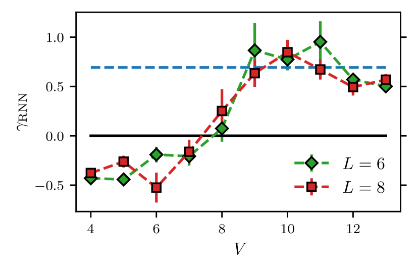
Figure 6: A plot of the topological entanglement entropy against the interaction strength $V$ (in units of $t$) of Hard-core Bose-Hubbard model on kagome lattice for system sizes $N=L\times L\times 3$ where $L=6,8$. The calculations were performed using the Kitaev-Preskill construction (see Fig. 2(c-d)). The continuous black horizontal line corresponds to a zero TEE, and the dashed blue horizontal line for a $\ln(2)$ TEE.

IV Conclusions and Outlooks

We have demonstrated a successful application of neural network wave functions to the task of detecting topological order in quantum systems. In particular, we use RNNs borrowed from natural language processing as ansatz wave functions. RNNs enjoy the autoregressive property which allows them to sample uncorrelated configurations. They are also capable of estimating second Renyi entropies using the swap trick Hibat-Allah et al. (2020) with which we computed TEEs using finite-size scaling and Kitaev-Preskill constructions Kitaev and Preskill (2006). Although we have fixed the size of the interior subregions $A$, $B$, $C$ to limit the error bars in our calculations, we note that it is possible to use improved estimators of TEE Hastings et al. (2010); Torlai et al. (2018); Wang and Davis (2020). Furthermore, the structural flexibility of the RNN offers the possibility to handle a wide variety of geometries including periodic boundary conditions in any spatial dimension which alleviate boundary effects on the TEE.

We have empirically demonstrated that 2D RNN wave functions support the 2D area law and can find a non-zero TEE for the toric code and for the hard-core Bose-Hubbard model on the Kagome lattice. We also find that RNNs favor coherent superpositions of MESs over a single MES. The success of our numerical experiments hinges on the combination of the exact sampling strategy used to compute observables, the structural properties of the RNN wave function, and the use of annealing as a strategy to overcome local minima during the optimization procedure.

The accuracy improvement of our findings can be achieved through the use of more advanced versions of RNNs and autoregressive models in general Hibat-Allah et al. ; Wu et al. (2022), or even a hybrid approach that combines QMC and RNNs Bennewitz et al. (2021); Czischek et al. (2022). Similarly, the incorporation of lattice symmetries provides a strategy to enhance the accuracy of our calculations Hibat-Allah et al. (2020, ); Nomura (2021). Although our results match the anticipated behavior of the toric code and Bose-Hubbard spin liquid models, we highlight that the RNN wave function may be susceptible to spurious contributions to the TEE Kim et al. (2023) and we have not addressed this issue in our work.

Finally, our methods can be applied to study other systems displaying topological order, such as the Rydberg atoms array Verresen et al. (2021); Semeghini et al. (2021); Giudici et al. (2022), either through variational methods or in combination with experimental data. To experimentally study topological order, it is possible to use quantum state tomography with RNNs Carrasquilla et al. (2019). This involves using experimental data to reconstruct the state seen in the experiment followed by an estimation of the TEE using the methods outlined in our work. Overall, our findings suggest that RNN wave function ansatzes have promising potential for discovering phases of matter with topological order.

Appendix A 2D periodic gated RNNs

In this appendix, we describe our implementation of a 2D gated RNN wave function for periodic systems, that can be used to approximate the ground states of the Hamiltonians considered in this paper. If we define

$$\bm{h^{\prime}}_{i,j} =[\bm{h}_{i-1,j};\bm{h}_{i,j-1};\bm{h}_{\text{mod}(i+1,L_{x}),j};\bm{h}_{i,\text{mod}(j+1,L_{y})}],$$

$$\bm{\sigma^{\prime}}_{i,j} =[\bm{\sigma}_{i-1,j};\bm{\sigma}_{i,j-1};\bm{\sigma}_{\text{mod}(i+1,L_{x}),j};\bm{\sigma}_{i,\text{mod}(j+1,L_{y})}],$$

then our gated 2D RNN wave function ansatz is based on the following recursion relations:

$$\tilde{\bm{h}}_{i,j} =\tanh\!\Big{(}W[\bm{\sigma^{\prime}}_{i,j};\bm{h^{\prime}}_{i,j}]+\bm{b}\Big{)},$$

$$\bm{u}_{i,j} =\text{sigmoid}\!\Big{(}W_{g}[\bm{\sigma^{\prime}}_{i,j};\bm{h^{\prime}}_{i,j}]+\bm{b}_{g}\Big{)},$$

$$\bm{h}_{i,j} =\bm{u}_{i,j}\odot\bm{\tilde{h}}_{i,j}+(1-\bm{u}_{i,j})\odot(U\bm{h^{\prime}}_{i,j}).$$

Here ‘$\odot$’ is the Hadamart (element-wise) product. A hidden state $\bm{h}_{i,j}$ can be obtained by combining a candidate state $\bm{\tilde{h}}_{i,j}$ and the neighboring hidden states $\bm{h}_{i-1,j},\bm{h}_{i,j-1},\bm{h}_{\text{mod}(i+1,L_{x}),j},\bm{h}_{i,\text{mod}(j+1,L_{y})}$. The update gate $\bm{u}_{i,j}$ determines how much of the candidate hidden state $\bm{\tilde{h}}_{i,j}$ will be taken into account and how much of the neighboring states will be considered. With this combination, it is possible to circumvent some limitations of the vanishing gradient problems Zhou et al. (2016); Shen (2019). The weight matrices $W,W_{g},U$ and the biases $b,b_{g}$ are variational parameters of our RNN ansatz. The size of the hidden state $\bm{h}_{i,j}$ is a hyperparameter called the number of memory units or the hidden dimension and is denoted as $d_{h}$. Finally, to motivate the use of the gating mechanism, we highlight that a gated 2D RNN was found to be better than a non-gated 2D RNN for the task of finding the ground state of a 2D Heisenberg model Hibat-Allah et al. .

Since we use an enlarged Hilbert space in our 2D RNN, we take $\bm{\sigma}_{ij}$ to be the concatenation of the one-hot encodings of the binary physical variables in each unit cell. In this case, if $m$ is the number of physical variables per unit cell, then $\bm{\sigma}_{ij}$ has size $2m$. We also note that the size of the Softmax layer is taken as $2^{m}$ so we can autoregressively sample each unit cell variables at once.

Appendix B Variational Monte Carlo and variance reduction

To optimize the energy expectation value of our RNN wave function $\ket{\Psi_{\bm{\theta}}}$, we use the Variational Monte Carlo (VMC) scheme, which consists of using importance sampling to estimate the expectation value of the energy $E_{\bm{\theta}}=\bra{\Psi_{\bm{\theta}}}\hat{H}\ket{\Psi_{\bm{\theta}}}$ as follows Becca and Sorella (2017); Hibat-Allah et al. (2020):

$$E_{\bm{\theta}}=\frac{1}{M}\sum_{i=1}^{M}E_{\text{loc}}(\bm{\sigma^{(i)}}),$$

where the local energies $E_{\text{loc}}$ are defined as

$$E_{\text{loc}}(\bm{\sigma})=\sum_{\bm{\sigma^{\prime}}}H_{\bm{\sigma}\bm{\sigma^{\prime}}}\frac{\Psi_{\bm{\theta}}(\bm{\sigma^{\prime}})}{\Psi_{\bm{\theta}}(\bm{\sigma})}.$$

Here the configurations $\{\bm{\sigma^{(i)}}\}_{i=1}^{M}$ are sampled from our ansatz using autoregressive sampling. The choice of $M$ is a hyperparameter that can be tuned. Furthermore, $E_{\text{loc}}(\bm{\sigma})$ can be efficiently computed for local Hamiltonians. Furthermore, the gradients can be estimated as Hibat-Allah et al. (2020)

$$\partial_{\bm{\theta}}E_{\bm{\theta}}=\frac{2}{M}\mathfrak{Re}\left(\sum_{i=1}^{M}\partial_{\bm{\theta}}\log\left(\Psi_{\bm{\theta}}^{*}(\bm{\sigma^{(i)}})\right)\left(E_{\text{loc}}(\bm{\sigma^{(i)}})-E_{\bm{\theta}}\right)\right).$$

For a stoquastic Hamiltonian $\hat{H}$ Bravyi (2015), we can use a positive RNN wave function where the use of the real part $\mathfrak{Re}$ is not necessary. Importantly, subtracting the variational energy $E_{\bm{\theta}}$ is helpful to achieve convergence as it reduces the variance of the gradients near convergence without biasing its expectation value as shown in Ref. Hibat-Allah et al. (2020). The subtracted term is referred to as a baseline, which is typically used for the same purpose in the context of Reinforcement learning Mohamed et al. (2019). To demonstrate the noise reduction more rigorously compared to the intuition provided in Ref. Hibat-Allah et al. (2020), let us focus on the variance of the gradient with respect to a parameter $\theta$ in the set of the variational parameters $\bm{\theta}$, after subtracting the baseline. Here we focus on the case of a positive ansatz wave function $\Psi_{\bm{\theta}}(\bm{\sigma})=\sqrt{P_{\bm{\theta}}(\bm{\sigma})}$ that we used in our study. First of all, we define:

$$O_{\theta}(\bm{\sigma})\equiv\partial_{\theta}\log\left(\Psi^{*}_{\bm{\theta}}(\bm{\sigma})\right)=\frac{1}{2}\partial_{\theta}\log(P_{\bm{\theta}}(\bm{\sigma})).$$

Thus, the gradient with a baseline can be written as:

$$\partial_{\theta}E_{\bm{\theta}} =2\left\langle O_{\theta}(\bm{\sigma})\overline{E}_{\text{loc}}(\bm{\sigma})\right\rangle,$$

where $\overline{E}_{\text{loc}}(\bm{\sigma})\equiv E_{\text{loc}}(\bm{\sigma})-E_{\bm{\theta}}$ and $\langle.\rangle$ denotes an expectation value over the Born distribution $|\Psi_{\bm{\theta}}(\bm{\sigma})|^{2}$. To estimate the gradients’ noise, we look at the variance of the gradient estimator, which can be decomposed as follows:

$$\text{Var}(O_{\theta}\overline{E}_{\text{loc}}) =\text{Var}(O_{\theta}E_{\text{loc}})$$

$$-2\text{Cov}(O_{\theta}E_{\text{loc}},O_{\theta}E_{\bm{\theta}})+E_{\bm{\theta}}^{2}\text{Var}(O_{\theta}).$$

Thus the variance reduction $R$, after subtracting the baseline, is given as:

$$R \equiv\text{Var}(O_{\theta}\overline{E}_{\text{loc}})-\text{Var}(O_{\theta}E_{\text{loc}}),$$

$$=-2E_{\bm{\theta}}\text{Cov}(O_{\theta}E_{\text{loc}},O_{\theta})+E_{\bm{\theta}}^{2}\text{Var}(O_{\theta}).$$

Since the gradients’ magnitude tends to near-zero values close to convergence, statistical errors are more likely to make the VMC optimization more challenging. We focus on this regime for this derivation to show the importance of the baseline in reducing noise. Thus, we assume that $E_{\text{loc}}(\bm{\sigma})=E_{\bm{\theta}}+\xi(\bm{\sigma})$, where the supremum of the local energy fluctuations is much smaller compared to the variational energy, i.e., $(\sup_{\bm{\sigma}}|\xi(\bm{\sigma})|)\ll E_{\bm{\theta}}$. From this assumption, we can deduce that:

$$R =-2E_{\bm{\theta}}^{2}\text{Cov}(O_{\theta},O_{\theta})$$ (11)

$$-2E_{\bm{\theta}}\text{Cov}(O_{\theta}\xi,O_{\theta})+E_{\bm{\theta}}^{2}\text{Var}(O_{\theta}),$$ (12)

$$=-E_{\bm{\theta}}^{2}\text{Var}(O_{\theta})-2E_{\bm{\theta}}\text{Cov}(O_{\theta}\xi,O_{\theta}).$$ (13)

The second term can be decomposed as follows:

$$\text{Cov}(O_{\theta}\xi,O_{\theta}) =\langle O_{\theta}^{2}\xi\rangle-\langle O_{\theta}\xi\rangle\langle O_{\theta}\rangle.$$ (14)

Since $\langle O_{\theta}\rangle=\frac{1}{2}\langle\partial_{\theta}\log(P_{\bm{\theta}})\rangle=0$ Sutton et al. (2000); Mohamed et al. (2019); Hibat-Allah et al. (2020), then we can bound the covariance term from above as:

$$\text{Cov}(O_{\theta}\xi,O_{\theta}) \leq\left(\sup_{\bm{\sigma}}|\xi(\bm{\sigma})|\right)\langle O_{\theta}^{2}\rangle,$$

$$=\left(\sup_{\bm{\sigma}}|\xi(\bm{\sigma})|\right)\text{Var}(O_{\theta}),$$

$$\ll E_{\bm{\theta}}\text{Var}(O_{\theta}).$$

Thus, we can conclude that the variance reduction $R$ in Eq. (13) is negative. This observation highlights the importance of the baseline in reducing the statistical noise of the energy gradients near convergence.

For a complex ansatz wave function $\Psi_{\bm{\theta}}(\bm{\sigma})=\sqrt{P_{\bm{\theta}}(\bm{\sigma})}\exp\left(\text{i}\phi_{\bm{\theta}}(\bm{\sigma})\right)$, the expectation value $\langle O_{\theta}\rangle=\frac{1}{2}\langle\partial_{\theta}\log(P_{\bm{\theta}})\rangle-\text{i}\langle\partial_{\theta}\phi_{\bm{\theta}}\rangle=-\text{i}\langle\partial_{\theta}\phi_{\bm{\theta}}\rangle$ is no longer equal zero in general. We leave the investigation of this case for future studies.

Similarly to the stochastic estimation of the variational energy using our ansatz, we can do the same for the estimation of the variational pseudo free energy $F_{\bm{\theta}}$ in Eq. (5). More details can be found in the supplementary information of Ref. Hibat-Allah et al. (2021). Finally, we note that the gradient steps in our numerical simulations are performed using Adam optimizer Kingma and Ba (2015).

Appendix C Hyperparameters

For all models studied in this paper, we note that for each annealing step, we perform $N_{\rm train}=5$ gradient steps. Concerning the learning rate $\eta$, we choose $\eta=10^{-3}$ during the warmup phase and the annealing phase and we switch to a learning rate $\eta=10^{-4}$ in the convergence phase. We finally note that we set the number of convergence steps as $N_{\rm convergence}=10000$. In Tab. 2, we provide further details about the hyperparameters we choose in our study for the different models. The meaning of each hyperparameter related to annealing is discussed in detail in Refs. Hibat-Allah et al. (2021, ).

Additionally, we use $M_{e}=2\times 10^{6}$ samples for the estimation of the entanglement entropy along with their error bars for the toric code. For the Bose-Hubbard model we use $M_{e}=10^{7}$ samples to reduce the error bars on the TEE in Fig. 6. To estimate the TEE uncertainty from the Kitaev-Preskill construction, we use the standard deviation expression of the sum of independent random variables Ku et al. (1966).

Finally, we note that to avoid fine-tuning the learning rate for each value of $V$ (between $4$ and $13$) in the Bose-Hubbard model, we target the normalized Hamiltonian

$$\hat{H}=-\frac{1}{V}\sum_{\langle i,j\rangle}\left(b_{i}^{\dagger}b_{j}+b_{i}b_{j}^{\dagger}\right)+\sum_{\hexagon}n_{\hexagon}^{2}$$ (15)

in our numerical experiments.

Figures	Parameter	Value
2D toric code	Number of memory units	$d_{h}=60$
	Number of samples	$M=100$
	Initial pseudo-temperature	$T_{0}=2$
	Number of annealing steps	$N_{\rm annealing}=4000$
Bose-Hubbard model (L = 6)	Number of memory units	$d_{h}=100$
	Number of samples	$M=500$
	Initial pseudo-temperature	$T_{0}=1$
	Number of annealing steps	$N_{\rm annealing}=10000$
Bose-Hubbard model (L = 8)	Number of memory units	$d_{h}=100$
	Number of samples	$M=500$
	Pseudo-temperature	$T_{0}=0$
	Number of steps	$10000$

Table 2: A summary of the hyperparameters used to obtain the results reported in this paper. Note that the number of samples $M$ corresponds to the batch size used during the training phase. Additionally, the $L=8$ RNN model is initialized with the $L=6$ optimized RNN for the Bose-Hubbard model.

References

- Sachdev (2011) Subir Sachdev, Quantum Phase Transitions, 2nd ed. (Cambridge University Press, 2011).
- Wen (2013) Xiao-Gang Wen, “Topological order: From long-range entangled quantum matter to a unified origin of light and electrons,” ISRN Condensed Matter Physics 2013, 1–20 (2013).
- Semeghini et al. (2021) G. Semeghini, H. Levine, A. Keesling, S. Ebadi, T. T. Wang, D. Bluvstein, R. Verresen, H. Pichler, M. Kalinowski, R. Samajdar, A. Omran, S. Sachdev, A. Vishwanath, M. Greiner, V. Vuletić, and M. D. Lukin, “Probing topological spin liquids on a programmable quantum simulator,” Science 374, 1242–1247 (2021).
- Satzinger et al. (2021) K. J. Satzinger, Y.-J Liu, A. Smith, C. Knapp, M. Newman, C. Jones, Z. Chen, C. Quintana, X. Mi, A. Dunsworth, C. Gidney, I. Aleiner, F. Arute, K. Arya, J. Atalaya, R. Babbush, J. C. Bardin, R. Barends, J. Basso, A. Bengtsson, A. Bilmes, M. Broughton, B. B. Buckley, D. A. Buell, B. Burkett, N. Bushnell, B. Chiaro, R. Collins, W. Courtney, S. Demura, A. R. Derk, D. Eppens, C. Erickson, L. Faoro, E. Farhi, A. G. Fowler, B. Foxen, M. Giustina, A. Greene, J. A. Gross, M. P. Harrigan, S. D. Harrington, J. Hilton, S. Hong, T. Huang, W. J. Huggins, L. B. Ioffe, S. V. Isakov, E. Jeffrey, Z. Jiang, D. Kafri, K. Kechedzhi, T. Khattar, S. Kim, P. V. Klimov, A. N. Korotkov, F. Kostritsa, D. Landhuis, P. Laptev, A. Locharla, E. Lucero, O. Martin, J. R. McClean, M. McEwen, K. C. Miao, M. Mohseni, S. Montazeri, W. Mruczkiewicz, J. Mutus, O. Naaman, M. Neeley, C. Neill, M. Y. Niu, T. E. O’Brien, A. Opremcak, B. Pató, A. Petukhov, N. C. Rubin, D. Sank, V. Shvarts, D. Strain, M. Szalay, B. Villalonga, T. C. White, Z. Yao, P. Yeh, J. Yoo, A. Zalcman, H. Neven, S. Boixo, A. Megrant, Y. Chen, J. Kelly, V. Smelyanskiy, A. Kitaev, M. Knap, F. Pollmann, and P. Roushan, “Realizing topologically ordered states on a quantum processor,” Science 374, 1237–1241 (2021).
- Dennis et al. (2002) Eric Dennis, Alexei Kitaev, Andrew Landahl, and John Preskill, “Topological quantum memory,” Journal of Mathematical Physics 43, 4452–4505 (2002).
- Kitaev (2006) Alexei Kitaev, “Anyons in an exactly solved model and beyond,” Annals of Physics January Special Issue, 321, 2–111 (2006).
- Kitaev and Laumann (2009) Alexei Kitaev and Chris Laumann, “Topological phases and quantum computation,” (2009), arXiv:0904.2771 [cond-mat.mes-hall] .
- Krinner et al. (2022) Sebastian Krinner, Nathan Lacroix, Ants Remm, Agustin Di Paolo, Elie Genois, Catherine Leroux, Christoph Hellings, Stefania Lazar, Francois Swiadek, Johannes Herrmann, Graham J. Norris, Christian Kraglund Andersen, Markus Müller, Alexandre Blais, Christopher Eichler, and Andreas Wallraff, “Realizing repeated quantum error correction in a distance-three surface code,” Nature 605, 669–674 (2022).
- Sivak et al. (2023) V. V. Sivak, A. Eickbusch, B. Royer, S. Singh, I. Tsioutsios, S. Ganjam, A. Miano, B. L. Brock, A. Z. Ding, L. Frunzio, S. M. Girvin, R. J. Schoelkopf, and M. H. Devoret, “Real-time quantum error correction beyond break-even,” Nature 616, 50–55 (2023).
- Acharya et al. (2023) Rajeev Acharya, Igor Aleiner, Richard Allen, Trond I. Andersen, Markus Ansmann, Frank Arute, Kunal Arya, Abraham Asfaw, Juan Atalaya, Ryan Babbush, Dave Bacon, Joseph C. Bardin, Joao Basso, Andreas Bengtsson, Sergio Boixo, Gina Bortoli, Alexandre Bourassa, Jenna Bovaird, Leon Brill, Michael Broughton, Bob B. Buckley, David A. Buell, Tim Burger, Brian Burkett, Nicholas Bushnell, Yu Chen, Zijun Chen, Ben Chiaro, Josh Cogan, Roberto Collins, Paul Conner, William Courtney, Alexander L. Crook, Ben Curtin, Dripto M. Debroy, Alexander Del Toro Barba, Sean Demura, Andrew Dunsworth, Daniel Eppens, Catherine Erickson, Lara Faoro, Edward Farhi, Reza Fatemi, Leslie Flores Burgos, Ebrahim Forati, Austin G. Fowler, Brooks Foxen, William Giang, Craig Gidney, Dar Gilboa, Marissa Giustina, Alejandro Grajales Dau, Jonathan A. Gross, Steve Habegger, Michael C. Hamilton, Matthew P. Harrigan, Sean D. Harrington, Oscar Higgott, Jeremy Hilton, Markus Hoffmann, Sabrina Hong, Trent Huang, Ashley Huff, William J. Huggins, Lev B. Ioffe, Sergei V. Isakov, Justin Iveland, Evan Jeffrey, Zhang Jiang, Cody Jones, Pavol Juhas, Dvir Kafri, Kostyantyn Kechedzhi, Julian Kelly, Tanuj Khattar, Mostafa Khezri, Mária Kieferová, Seon Kim, Alexei Kitaev, Paul V. Klimov, Andrey R. Klots, Alexander N. Korotkov, Fedor Kostritsa, John Mark Kreikebaum, David Landhuis, Pavel Laptev, Kim-Ming Lau, Lily Laws, Joonho Lee, Kenny Lee, Brian J. Lester, Alexander Lill, Wayne Liu, Aditya Locharla, Erik Lucero, Fionn D. Malone, Jeffrey Marshall, Orion Martin, Jarrod R. McClean, Trevor McCourt, Matt McEwen, Anthony Megrant, Bernardo Meurer Costa, Xiao Mi, Kevin C. Miao, Masoud Mohseni, Shirin Montazeri, Alexis Morvan, Emily Mount, Wojciech Mruczkiewicz, Ofer Naaman, Matthew Neeley, Charles Neill, Ani Nersisyan, Hartmut Neven, Michael Newman, Jiun How Ng, Anthony Nguyen, Murray Nguyen, Murphy Yuezhen Niu, Thomas E. O’Brien, Alex Opremcak, John Platt, Andre Petukhov, Rebecca Potter, Leonid P. Pryadko, Chris Quintana, Pedram Roushan, Nicholas C. Rubin, Negar Saei, Daniel Sank, Kannan Sankaragomathi, Kevin J. Satzinger, Henry F. Schurkus, Christopher Schuster, Michael J. Shearn, Aaron Shorter, Vladimir Shvarts, Jindra Skruzny, Vadim Smelyanskiy, W. Clarke Smith, George Sterling, Doug Strain, Marco Szalay, Alfredo Torres, Guifre Vidal, Benjamin Villalonga, Catherine Vollgraff Heidweiller, Theodore White, Cheng Xing, Z. Jamie Yao, Ping Yeh, Juhwan Yoo, Grayson Young, Adam Zalcman, Yaxing Zhang, Ningfeng Zhu, and Google Quantum AI, “Suppressing quantum errors by scaling a surface code logical qubit,” Nature 614, 676–681 (2023).
- Levin and Wen (2006) Michael Levin and Xiao-Gang Wen, “Detecting topological order in a ground state wave function,” Physical Review Letters 96 (2006), 10.1103/physrevlett.96.110405.
- Kitaev and Preskill (2006) Alexei Kitaev and John Preskill, “Topological entanglement entropy,” Phys. Rev. Lett. 96, 110404 (2006).
- Hamma et al. (2005a) Alioscia Hamma, Radu Ionicioiu, and Paolo Zanardi, “Bipartite entanglement and entropic boundary law in lattice spin systems,” Physical Review A 71 (2005a), 10.1103/physreva.71.022315.
- Isakov et al. (2011) Sergei V. Isakov, Matthew B. Hastings, and Roger G. Melko, “Topological entanglement entropy of a bose–hubbard spin liquid,” Nature Physics 7, 772–775 (2011).
- Wildeboer et al. (2017) Julia Wildeboer, Alexander Seidel, and Roger G. Melko, “Entanglement entropy and topological order in resonating valence-bond quantum spin liquids,” Physical Review B 95 (2017), 10.1103/physrevb.95.100402.
- Zhao et al. (2022) Jiarui Zhao, Bin-Bin Chen, Yan-Cheng Wang, Zheng Yan, Meng Cheng, and Zi Yang Meng, “Measuring rényi entanglement entropy with high efficiency and precision in quantum monte carlo simulations,” npj Quantum Materials 7 (2022), 10.1038/s41535-022-00476-0.
- Jiang et al. (2012) Hong-Chen Jiang, Zhenghan Wang, and Leon Balents, “Identifying topological order by entanglement entropy,” Nature Physics 8, 902–905 (2012).
- Jiang and Balents (2013) Hong-Chen Jiang and Leon Balents, “Collapsing schrödinger cats in the density matrix renormalization group,” (2013), 10.48550/ARXIV.1309.7438.
- Carrasquilla and Melko (2017) Juan Carrasquilla and Roger G. Melko, “Machine learning phases of matter,” Nature Physics 13, 431–434 (2017).
- Broecker et al. (2017) Peter Broecker, Juan Carrasquilla, Roger G. Melko, and Simon Trebst, “Machine learning quantum phases of matter beyond the fermion sign problem,” Scientific Reports 7, 8823 (2017).
- Ch’ng et al. (2017) Kelvin Ch’ng, Juan Carrasquilla, Roger G. Melko, and Ehsan Khatami, “Machine learning phases of strongly correlated fermions,” Phys. Rev. X 7, 031038 (2017).
- Miles et al. (2021) Cole Miles, Rhine Samajdar, Sepehr Ebadi, Tout T. Wang, Hannes Pichler, Subir Sachdev, Mikhail D. Lukin, Markus Greiner, Kilian Q. Weinberger, and Eun-Ah Kim, “Machine learning discovery of new phases in programmable quantum simulator snapshots,” (2021), 10.48550/ARXIV.2112.10789.
- Torlai et al. (2018) Giacomo Torlai, Guglielmo Mazzola, Juan Carrasquilla, Matthias Troyer, Roger Melko, and Giuseppe Carleo, “Neural-network quantum state tomography,” Nature Physics 14, 447–450 (2018).
- Carrasquilla et al. (2019) Juan Carrasquilla, Giacomo Torlai, Roger G. Melko, and Leandro Aolita, “Reconstructing quantum states with generative models,” Nature Machine Intelligence 1, 155–161 (2019).
- Androsiuk et al. (1993) J. Androsiuk, L. Kulak, and K. Sienicki, “Neural network solution of the Schrödinger equation for a two-dimensional harmonic oscillator,” Chemical Physics 173, 377–383 (1993).
- LAG (1997) “Artificial neural network methods in quantum mechanics,” Computer Physics Communications 104, 1 – 14 (1997).
- Carleo and Troyer (2017) Giuseppe Carleo and Matthias Troyer, “Solving the quantum many-body problem with artificial neural networks,” Science 355, 602–606 (2017).
- Cai and Liu (2018) Zi Cai and Jinguo Liu, “Approximating quantum many-body wave functions using artificial neural networks,” Phys. Rev. B 97, 035116 (2018).
- Luo and Clark (2019) Di Luo and Bryan K. Clark, “Backflow transformations via neural networks for quantum many-body wave functions,” Phys. Rev. Lett. 122, 226401 (2019).
- Pfau et al. (2020) David Pfau, James S. Spencer, Alexander G. D. G. Matthews, and W. M. C. Foulkes, “Ab initio solution of the many-electron schrödinger equation with deep neural networks,” Physical Review Research 2 (2020), 10.1103/physrevresearch.2.033429.
- Hermann et al. (2020) Jan Hermann, Zeno Schätzle, and Frank Noé, “Deep-neural-network solution of the electronic schrödinger equation,” Nature Chemistry 12, 891–897 (2020).
- Choo et al. (2020) Kenny Choo, Antonio Mezzacapo, and Giuseppe Carleo, “Fermionic neural-network states for ab-initio electronic structure,” Nature Communications 11, 2368 (2020).
- Hibat-Allah et al. (2020) Mohamed Hibat-Allah, Martin Ganahl, Lauren E. Hayward, Roger G. Melko, and Juan Carrasquilla, “Recurrent neural network wave functions,” Physical Review Research 2 (2020), 10.1103/physrevresearch.2.023358.
- Roth (2020) Christopher Roth, “Iterative retraining of quantum spin models using recurrent neural networks,” (2020), arXiv:2003.06228 [physics.comp-ph] .
- Vicentini et al. (2019) Filippo Vicentini, Alberto Biella, Nicolas Regnault, and Cristiano Ciuti, “Variational neural-network ansatz for steady states in open quantum systems,” Phys. Rev. Lett. 122, 250503 (2019).
- Luo et al. (2022) Di Luo, Zhuo Chen, Juan Carrasquilla, and Bryan K. Clark, “Autoregressive neural network for simulating open quantum systems via a probabilistic formulation,” Phys. Rev. Lett. 128, 090501 (2022).
- Jónsson et al. (2018) Bjarni Jónsson, Bela Bauer, and Giuseppe Carleo, “Neural-network states for the classical simulation of quantum computing,” (2018), 10.48550/ARXIV.1808.05232.
- Medvidović and Carleo (2021) Matija Medvidović and Giuseppe Carleo, “Classical variational simulation of the quantum approximate optimization algorithm,” npj Quantum Information 7, 101 (2021).
- Carrasquilla et al. (2021) Juan Carrasquilla, Di Luo, Felipe Pérez, Ashley Milsted, Bryan K. Clark, Maksims Volkovs, and Leandro Aolita, “Probabilistic simulation of quantum circuits using a deep-learning architecture,” Phys. Rev. A 104, 032610 (2021).
- Dunjko and Briegel (2018) Vedran Dunjko and Hans J. Briegel, “Machine learning & artificial intelligence in the quantum domain: A review of recent progress,” Reports on Progress in Physics 81, 074001 (2018).
- Carleo et al. (2019) Giuseppe Carleo, Ignacio Cirac, Kyle Cranmer, Laurent Daudet, Maria Schuld, Naftali Tishby, Leslie Vogt-Maranto, and Lenka Zdeborová, “Machine learning and the physical sciences,” Rev. Mod. Phys. 91, 045002 (2019).
- Carrasquilla (2020) Juan Carrasquilla, “Machine learning for quantum matter,” Advances in Physics: X 5, 1797528 (2020).
- Dawid et al. (2022) Anna Dawid, Julian Arnold, Borja Requena, Alexander Gresch, Marcin Płodzień, Kaelan Donatella, Kim A. Nicoli, Paolo Stornati, Rouven Koch, Miriam Büttner, Robert Okuła, Gorka Muñoz-Gil, Rodrigo A. Vargas-Hernández, Alba Cervera-Lierta, Juan Carrasquilla, Vedran Dunjko, Marylou Gabrié, Patrick Huembeli, Evert van Nieuwenburg, Filippo Vicentini, Lei Wang, Sebastian J. Wetzel, Giuseppe Carleo, Eliška Greplová, Roman Krems, Florian Marquardt, Michał Tomza, Maciej Lewenstein, and Alexandre Dauphin, “Modern applications of machine learning in quantum sciences,” (2022), 10.48550/arXiv.2204.04198, arXiv:2204.04198 [cond-mat, physics:quant-ph] .
- Deng et al. (2017) Dong-Ling Deng, Xiaopeng Li, and S. Das Sarma, “Machine learning topological states,” Physical Review B 96 (2017), 10.1103/physrevb.96.195145.
- Glasser et al. (2018) Ivan Glasser, Nicola Pancotti, Moritz August, Ivan D. Rodriguez, and J. Ignacio Cirac, “Neural-network quantum states, string-bond states, and chiral topological states,” Physical Review X 8 (2018), 10.1103/physrevx.8.011006.
- Chen et al. (2018) Jing Chen, Song Cheng, Haidong Xie, Lei Wang, and Tao Xiang, “Equivalence of restricted Boltzmann machines and tensor network states,” Physical Review B 97, 085104 (2018).
- Lu et al. (2019) Sirui Lu, Xun Gao, and L.-M. Duan, “Efficient representation of topologically ordered states with restricted boltzmann machines,” Phys. Rev. B 99, 155136 (2019).
- Luo et al. (2021) Di Luo, Zhuo Chen, Kaiwen Hu, Zhizhen Zhao, Vera Mikyoung Hur, and Bryan K. Clark, “Gauge invariant autoregressive neural networks for quantum lattice models,” (2021), arXiv:2101.07243 [cond-mat.str-el] .
- Hochreiter and Schmidhuber (1997) Sepp Hochreiter and Jürgen Schmidhuber, “Long short-term memory,” Neural Comput. 9, 1735–1780 (1997).
- Graves (2012) Alex Graves, “Supervised sequence labelling,” in Supervised sequence labelling with recurrent neural networks (Springer, 2012) pp. 5–13.
- Lipton et al. (2015) Zachary C. Lipton, John Berkowitz, and Charles Elkan, “A critical review of recurrent neural networks for sequence learning,” (2015), arXiv:1506.00019 [cs.LG] .
- Isakov et al. (2006) S. V. Isakov, Yong Baek Kim, and A. Paramekanti, “Spin-liquid phase in a spin- quantum magnet on the kagome lattice,” Phys. Rev. Lett. 97, 207204 (2006).
- Bravyi (2015) Sergey Bravyi, “Monte carlo simulation of stoquastic hamiltonians,” (2015), arXiv:1402.2295 [quant-ph] .
- Ferris and Vidal (2012) Andrew J. Ferris and Guifre Vidal, “Perfect sampling with unitary tensor networks,” Physical Review B 85 (2012), 10.1103/physrevb.85.165146.
- Graves et al. (2007) Alex Graves, Santiago Fernandez, and Juergen Schmidhuber, “Multi-dimensional recurrent neural networks,” (2007), arXiv:0705.2011 [cs.AI] .
- Jain et al. (2020) Ajay Jain, Pieter Abbeel, and Deepak Pathak, “Locally masked convolution for autoregressive models,” (2020), arXiv:2006.12486 [cs.LG] .
- Casert et al. (2021) Corneel Casert, Tom Vieijra, Stephen Whitelam, and Isaac Tamblyn, “Dynamical large deviations of two-dimensional kinetically constrained models using a neural-network state ansatz,” Phys. Rev. Lett. 127, 120602 (2021).
- (58) Mohamed Hibat-Allah, Roger G Melko, and Juan Carrasquilla, “Supplementing recurrent neural network wave functions with symmetry and annealing to improve accuracy,” Machine Learning and the Physical Sciences (NeurIPS 2021) .
- Haferkamp et al. (2020) Jonas Haferkamp, Dominik Hangleiter, Jens Eisert, and Marek Gluza, “Contracting projected entangled pair states is average-case hard,” Physical Review Research 2 (2020), 10.1103/physrevresearch.2.013010.
- Vanderstraeten et al. (2016) Laurens Vanderstraeten, Jutho Haegeman, Philippe Corboz, and Frank Verstraete, “Gradient methods for variational optimization of projected entangled-pair states,” Physical Review B 94 (2016), 10.1103/physrevb.94.155123.
- Becca and Sorella (2017) Federico Becca and Sandro Sorella, Quantum Monte Carlo Approaches for Correlated Systems (Cambridge University Press, 2017).
- Hibat-Allah et al. (2021) Mohamed Hibat-Allah, Estelle M. Inack, Roeland Wiersema, Roger G. Melko, and Juan Carrasquilla, “Variational neural annealing,” Nature Machine Intelligence (2021), 10.1038/s42256-021-00401-3.
- Bukov et al. (2021) Marin Bukov, Markus Schmitt, and Maxime Dupont, “Learning the ground state of a non-stoquastic quantum hamiltonian in a rugged neural network landscape,” SciPost Physics 10 (2021), 10.21468/scipostphys.10.6.147.
- Roth et al. (2022) Christopher Roth, Attila Szabó, and Allan MacDonald, “High-accuracy variational monte carlo for frustrated magnets with deep neural networks,” (2022), 10.48550/ARXIV.2211.07749.
- Khandoker et al. (2023) Shoummo Ahsan Khandoker, Jawaril Munshad Abedin, and Mohamed Hibat-Allah, “Supplementing recurrent neural networks with annealing to solve combinatorial optimization problems,” Machine Learning: Science and Technology 4, 015026 (2023).
- Hamma et al. (2005b) Alioscia Hamma, Radu Ionicioiu, and Paolo Zanardi, “Ground state entanglement and geometric entropy in the kitaev model,” Physics Letters A 337, 22–28 (2005b).
- Flammia et al. (2009) Steven T. Flammia, Alioscia Hamma, Taylor L. Hughes, and Xiao-Gang Wen, “Topological entanglement rényi entropy and reduced density matrix structure,” Physical Review Letters 103 (2009), 10.1103/physrevlett.103.261601.
- Zhang et al. (2012) Yi Zhang, Tarun Grover, Ari Turner, Masaki Oshikawa, and Ashvin Vishwanath, “Quasiparticle statistics and braiding from ground-state entanglement,” Physical Review B 85 (2012), 10.1103/physrevb.85.235151.
- Kim et al. (2023) Isaac H. Kim, Michael Levin, Ting-Chun Lin, Daniel Ranard, and Bowen Shi, “Universal lower bound on topological entanglement entropy,” (2023), arXiv:2302.00689 [cond-mat, physics:quant-ph] .
- Hastings et al. (2010) Matthew B. Hastings, Iván González, Ann B. Kallin, and Roger G. Melko, “Measuring renyi entanglement entropy in quantum monte carlo simulations,” Physical Review Letters 104 (2010), 10.1103/physrevlett.104.157201.
- Wang and Davis (2020) Zhaoyou Wang and Emily J. Davis, “Calculating rényi entropies with neural autoregressive quantum states,” Physical Review A 102 (2020), 10.1103/physreva.102.062413.
- Furukawa and Misguich (2007) Shunsuke Furukawa and Grégoire Misguich, “Topological entanglement entropy in the quantum dimer model on the triangular lattice,” Physical Review B 75 (2007), 10.1103/physrevb.75.214407.
- Stoudenmire and White (2012) E.M. Stoudenmire and Steven R. White, “Studying two-dimensional systems with the density matrix renormalization group,” Annual Review of Condensed Matter Physics 3, 111–128 (2012).
- Gong et al. (2014) Shou-Shu Gong, Wei Zhu, D. N. Sheng, Olexei I. Motrunich, and Matthew P. A. Fisher, “Plaquette ordered phase and quantum phase diagram in the spin- square heisenberg model,” Phys. Rev. Lett. 113, 027201 (2014).
- Samajdar et al. (2021) Rhine Samajdar, Wen Wei Ho, Hannes Pichler, Mikhail D. Lukin, and Subir Sachdev, “Quantum phases of rydberg atoms on a kagome lattice,” Proceedings of the National Academy of Sciences 118, e2015785118 (2021).
- Milsted et al. (2019) Ashley Milsted, Martin Ganahl, Stefan Leichenauer, Jack Hidary, and Guifre Vidal, “Tensornetwork on tensorflow: A spin chain application using tree tensor networks,” (2019), 10.48550/ARXIV.1905.01331.
- Wu et al. (2022) Dian Wu, Riccardo Rossi, Filippo Vicentini, and Giuseppe Carleo, “From tensor network quantum states to tensorial recurrent neural networks,” (2022), 10.48550/ARXIV.2206.12363.
- Note (1) Note that this choice allows minimizing the boundary size as opposed to a square region in the bulk. This feature is desirable since the swap operator used to estimate the second Renyi entropy Hibat-Allah et al. (2020) becomes very small, and thus more sensitive to statistical errors when the boundary increases for a quantum system satisfying the area law.
- Fradkin (2013) Eduardo Fradkin, Field Theories of Condensed Matter Physics, 2nd ed. (Cambridge University Press, 2013).
- Wang et al. (2017) Yan-Cheng Wang, Chen Fang, Meng Cheng, Yang Qi, and Zi Yang Meng, “Topological Spin Liquid with Symmetry-Protected Edge States,” (2017), arXiv:1701.01552 [cond-mat] .
- Kulchytskyy et al. (2015) Bohdan Kulchytskyy, C. M. Herdman, Stephen Inglis, and Roger G. Melko, “Detecting goldstone modes with entanglement entropy,” Physical Review B 92 (2015), 10.1103/physrevb.92.115146.
- Bennewitz et al. (2021) Elizabeth R. Bennewitz, Florian Hopfmueller, Bohdan Kulchytskyy, Juan Felipe Carrasquilla, and Pooya Ronagh, “Neural error mitigation of near-term quantum simulations,” ArXiv (2021), 2105.08086 .
- Czischek et al. (2022) Stefanie Czischek, M. Schuyler Moss, Matthew Radzihovsky, Ejaaz Merali, and Roger G. Melko, “Data-enhanced variational monte carlo simulations for rydberg atom arrays,” Physical Review B 105 (2022), 10.1103/physrevb.105.205108.
- Nomura (2021) Yusuke Nomura, “Helping restricted boltzmann machines with quantum-state representation by restoring symmetry,” Journal of Physics: Condensed Matter 33, 174003 (2021).
- Verresen et al. (2021) Ruben Verresen, Mikhail D. Lukin, and Ashvin Vishwanath, “Prediction of toric code topological order from rydberg blockade,” Physical Review X 11 (2021), 10.1103/physrevx.11.031005.
- Giudici et al. (2022) Giuliano Giudici, Mikhail D Lukin, and Hannes Pichler, “Dynamical preparation of quantum spin liquids in rydberg atom arrays,” (2022), arXiv:2202.09372 [quant-ph] .
- Abadi et al. (2015) Martín Abadi, Ashish Agarwal, Paul Barham, Eugene Brevdo, Zhifeng Chen, Craig Citro, Greg S. Corrado, Andy Davis, Jeffrey Dean, Matthieu Devin, Sanjay Ghemawat, Ian Goodfellow, Andrew Harp, Geoffrey Irving, Michael Isard, Yangqing Jia, Rafal Jozefowicz, Lukasz Kaiser, Manjunath Kudlur, Josh Levenberg, Dandelion Mané, Rajat Monga, Sherry Moore, Derek Murray, Chris Olah, Mike Schuster, Jonathon Shlens, Benoit Steiner, Ilya Sutskever, Kunal Talwar, Paul Tucker, Vincent Vanhoucke, Vijay Vasudevan, Fernanda Viégas, Oriol Vinyals, Pete Warden, Martin Wattenberg, Martin Wicke, Yuan Yu, and Xiaoqiang Zheng, “TensorFlow: Large-scale machine learning on heterogeneous systems,” (2015), software available from tensorflow.org.
- Harris et al. (2020) Charles R. Harris, K. Jarrod Millman, Stéfan J. van der Walt, Ralf Gommers, Pauli Virtanen, David Cournapeau, Eric Wieser, Julian Taylor, Sebastian Berg, Nathaniel J. Smith, Robert Kern, Matti Picus, Stephan Hoyer, Marten H. van Kerkwijk, Matthew Brett, Allan Haldane, Jaime Fernández del Río, Mark Wiebe, Pearu Peterson, Pierre Gérard-Marchant, Kevin Sheppard, Tyler Reddy, Warren Weckesser, Hameer Abbasi, Christoph Gohlke, and Travis E. Oliphant, “Array programming with numpy,” Nature 585, 357–362 (2020).
- Zhou et al. (2016) Guo-Bing Zhou, Jianxin Wu, Chen-Lin Zhang, and Zhi-Hua Zhou, “Minimal gated unit for recurrent neural networks,” (2016), arXiv:1603.09420 [cs.NE] .
- Shen (2019) Huitao Shen, “Mutual information scaling and expressive power of sequence models,” (2019), arXiv:1905.04271 [cs.LG] .
- Mohamed et al. (2019) Shakir Mohamed, Mihaela Rosca, Michael Figurnov, and Andriy Mnih, “Monte carlo gradient estimation in machine learning,” (2019), arXiv:1906.10652 [stat.ML] .
- Sutton et al. (2000) Richard S Sutton, David A McAllester, Satinder P Singh, and Yishay Mansour, “Policy gradient methods for reinforcement learning with function approximation,” in Advances in neural information processing systems (2000) pp. 1057–1063.
- Kingma and Ba (2015) Diederik P. Kingma and Jimmy Ba, “Adam: A method for stochastic optimization,” in 3rd International Conference on Learning Representations, ICLR 2015, San Diego, CA, USA, May 7-9, 2015, Conference Track Proceedings, edited by Yoshua Bengio and Yann LeCun (2015).
- Ku et al. (1966) Harry H Ku et al., “Notes on the use of propagation of error formulas,” Journal of Research of the National Bureau of Standards 70 (1966).