Entropy-dissipation Informed Neural Network
for McKean-Vlasov Type PDEs

Abstract

The McKean-Vlasov equation (MVE) describes the collective behavior of particles subject to drift, diffusion, and mean-field interaction. In physical systems, the interaction term can be singular, i.e. it diverges when two particles collide. Notable examples of such interactions include the Coulomb interaction, fundamental in plasma physics, and the Biot-Savart interaction, present in the vorticity formulation of the 2D Navier-Stokes equation (NSE) in fluid dynamics. Solving MVEs that involve singular interaction kernels presents a significant challenge, especially when aiming to provide rigorous theoretical guarantees. In this work, we propose a novel approach based on the concept of entropy dissipation in the underlying system. We derive a potential function that effectively controls the KL divergence between a hypothesis solution and the ground truth. Building upon this theoretical foundation, we introduce the Entropy-dissipation Informed Neural Network (EINN) framework for solving MVEs. In EINN, we utilize neural networks (NN) to approximate the underlying velocity field and minimize the proposed potential function. By leveraging the expressive power of NNs, our approach offers a promising avenue for tackling the complexities associated with singular interactions. To assess the empirical performance of our method, we compare EINN with SOTA NN-based MVE solvers. The results demonstrate the effectiveness of our approach in solving MVEs across various example problems.

1 Introduction

Scientists use Partial Differential Equations (PDEs) to describe natural laws and predict the dynamics of real-world systems. As PDEs are of fundamental importance, a growing area in machine learning is the use of neural networks (NN) to solve these equations (Han et al., 2018; Zhang et al., 2018; Raissi et al., 2020; Cai et al., 2021; Karniadakis et al., 2021; Cuomo et al., 2022). An important category of PDEs is the McKean-Vlasov equation (MVE), which models the dynamics of a stochastic particle system with mean-field interactions

$$\mathrm{d}{\mathbf{X}}_{t}=-\nabla V({\mathbf{X}}_{t})\mathrm{d}t+K\ast\bar{\rho}_{t}({\mathbf{X}}_{t})\mathrm{d}t+\sqrt{2\nu}\mathrm{d}{\mathbf{B}}_{t},\quad\bar{\rho}_{t}=\mathrm{Law}({\mathbf{X}}_{t}).$$ (1)

Here ${\mathbf{X}}_{t}\in\mathcal{X}$ denotes a random particle’ position, $\mathcal{X}$ is either $\mathbb{R}^{d}$ or the torus $\Pi^{d}$ (a cube $[-L,L]^{d}$ with periodic boundary condition), $V:{\mathbb{R}}^{d}\rightarrow{\mathbb{R}}$ denotes a known potential, $K:{\mathbb{R}}^{d}\rightarrow{\mathbb{R}}^{d}$ denotes some interaction kernel and the convolution operation is defined as $h\ast\phi=\int_{\mathcal{X}}h({\bm{x}}-{\bm{y}})\phi({\bm{y}})d{\bm{y}}$, $\{{\mathbf{B}}_{t}\}_{t\geq 0}$ is the standard $d$-dimensional Wiener process with $\nu\geq 0$ being the diffusion coefficient, and $\bar{\rho}_{t}:\mathcal{X}\rightarrow{\mathbb{R}}$ is the law or the probability density function of the random variable ${\mathbf{X}}_{t}$ and the initial data $\bar{\rho}_{0}$ is given. Under mild regularity conditions, the density function $\bar{\rho}_{t}$ satisfies the MVE

$$\text{(MVE)}\quad\partial_{t}\bar{\rho}_{t}({\bm{x}})+\,\mathrm{div}\left(\bar{\rho}_{t}(-\nabla V({\bm{x}})+K\ast\bar{\rho}_{t}({\bm{x}}))\right)=\nu\Delta\bar{\rho}_{t}({\bm{x}}),$$ (2)

where $\,\mathrm{div}$ denotes the divergence operator, $\,\mathrm{div}\ h({\bm{x}})=\sum_{i=1}^{d}{\partial h_{i}}/{\partial x_{i}}$ for a velocity field $h:{\mathbb{R}}^{d}\rightarrow{\mathbb{R}}^{d}$, $\Delta$ denotes the Laplacian operator defined as $\Delta\phi=\,\mathrm{div}(\nabla\phi)$, where $\nabla\phi$ denotes the gradient of a scalar function $\phi:{\mathbb{R}}^{d}\rightarrow{\mathbb{R}}$. Note that all these operators are applied only on the spatial variable ${\bm{x}}$.

In order to describe dynamics in real-world phenomena such as electromagnetism (Golse, 2016) and fluid mechanics (Majda et al., 2002), the interaction kernels $K$ in the MVE can be highly singular, i.e. $\|K({\bm{x}})\|\rightarrow\infty$ when $\|{\bm{x}}\|\rightarrow 0$. Two of the most notable examples are the Coulomb interactions

$$\text{(Coulomb Kernel)}\quad K({\bm{x}})=-\nabla g({\bm{x}}),\ \mathrm{with}\ g({\bm{x}})=\begin{cases}\left((d-2)S_{d-1}(1)\right)^{-1}\|{\bm{x}}\|^{-(d-2)},&d\geq 3,\\ -(2\pi)^{-1}\log\|{\bm{x}}\|,&d=2,\end{cases}$$ (3)

with $S_{d-1}(1)$ denoting the surface area of the unit sphere in ${\mathbb{R}}^{d}$, and the vorticity formulation of the 2D Navier-Stokes equation (NSE) where the interaction kernel $K$ is given by the Biot-Savart law

$$\text{(Biot-Savart Kernel)}\quad K({\bm{x}})=\frac{1}{2\pi}\frac{{\bm{x}}^{\perp}}{\|{\bm{x}}\|^{2}}=\frac{1}{2\pi}\left(-\frac{x_{2}}{\|{\bm{x}}\|^{2}},\frac{x_{1}}{\|{\bm{x}}\|^{2}}\right),$$ (4)

where ${\bm{x}}=(x_{1},x_{2})$ and $\|{\bm{x}}\|$ denotes the Euclidean norm of a vector.
Classical methods for solving MVEs, including finite difference, finite volume, finite element, spectral methods, and particle methods, have been developed over time. A common drawback of these methods lies in the constraints of their solution representation: Sparse representations, such as less granular grids, cells, meshes, fewer basis functions, or particles, may lead to an inferior solution accuracy; On the other hand, dense representations incur higher computational and memory costs.
As a potent tool for function approximation, NNs are anticipated to overcome these hurdles and handle higher-dimensional, less regular, and more complex systems efficiently (Weinan et al., 2021). The most renowned NN-based algorithm is the Physics Informed Neural Network (PINN) (Raissi et al., 2019). The philosophy behind the PINN method is that solving a PDE system is equivalent to finding the root of the corresponding differential operators. PINN tackles the latter problem by directly parameterizing the hypothesis solution with an NN and training it to minimize the ${\mathcal{L}}^{2}$ functional residual of the operators. As a versatile PDE solver, PINN may fail to exploit the underlying dynamics of the PDE, which possibly leads to inferior performance on task-specific solvers. For example, on the 2D NSE problem, a recent NN-based development Zhang et al. (2022) surpasses PINN and sets a new SOTA empirical performance, which however lacks rigorous theoretical substantiation. Despite the widespread applications of PINN, rigorous error estimation guarantees are scarce in the literature. While we could not find results on the MVE with the Coulomb interaction, only in a very recent paper (De Ryck et al., 2023), the authors establish for NSE that the PINN loss controls the discrepancy between a candidate solution and the ground truth. We highlight that their result holds average-in-time, meaning that at a particular timestamp $t\in[0,T]$, a candidate solution with small PINN loss may still significantly differ from the true solution. In contrast, all guarantees in this paper are uniform-in-time. Moreover, there is a factor in the aforementioned guarantee that exponentially depends on the total evolving time $T$, while the factor in our guarantee for the NSE is independent of $T$. We highlight that these novel improvements are achieved for the proposed EINN framework since we take a completely different route from PINN: Our approach is explicitly designed to exploit the underlying dynamics of the system, as elaborated below.

Our approach

Define the operator

$$\mathcal{A}[\rho]\overset{\operatorname{def}}{=}-\nabla V+K\ast\rho-\nu\nabla\log\rho.$$ (5)

By noting $\Delta\bar{\rho}_{t}=\,\mathrm{div}(\bar{\rho}_{t}\nabla\log\bar{\rho}_{t})$, we can rewrite the MVE in the form of a continuity equation

$$\partial_{t}\bar{\rho}_{t}({\bm{x}})+\,\mathrm{div}\Big{(}\bar{\rho}_{t}({\bm{x}}){\mathcal{A}}[\bar{\rho}_{t}]({\bm{x}})\Big{)}=0.$$ (6)

For simplicity, we will refer to $\mathcal{A}[\bar{\rho}_{t}]$ as the underlying velocity. Consider another time-varying hypothesis velocity field $f:{\mathbb{R}}\times{\mathbb{R}}^{d}\rightarrow{\mathbb{R}}$ and let $\rho^{f}_{t}$ be the solution to the continuity equation

$$\text{(hypothesis solution)}\quad\partial_{t}\rho^{f}_{t}({\bm{x}})+\,\mathrm{div}(\rho_{t}^{f}({\bm{x}})f(t,{\bm{x}}))=0,\ \rho^{f}_{0}=\bar{\rho}_{0}$$ (7)

for $t\in[0,T]$, where we recall that the initial law $\bar{\rho}_{0}$ is known. We will refer to $\rho_{t}^{f}$ as the hypothesis solution and use the superscript to emphasize its dependence on the hypothesis velocity field $f$. We propose an Entropy-dissipation Informed Neural Network framework (EINN), which trains an NN parameterized hypothesis velocity field $f_{\theta}$ by minimizing the following EINN loss

$$\text{({EINN}\ loss)}\quad R(f_{\theta})\overset{\operatorname{def}}{=}\int_{0}^{T}\int_{\mathcal{X}}\|f_{\theta}(t,{\bm{x}})-\mathcal{A}[\rho_{t}^{f_{\theta}}]({\bm{x}})\|^{2}{\rho_{t}^{f_{\theta}}}({\bm{x}})\mathrm{d}{\bm{x}}\mathrm{d}t.$$ (8)

The objective (8) is obtained by studying the stability of carefully constructed Lyapunov functions. These Lyapunov functions draw inspiration from the concept of entropy dissipation in the system, leading to the name of our framework. We highlight that we provide a rigorous error estimation guarantee for our framework for MVEs with singular kernels (3) and (4), showing that when $R(f_{\theta})$ is sufficiently small, $\rho_{t}^{f_{\theta}}$ recovers the ground truth $\bar{\rho}_{t}$ in the KL sense, uniform in time.

Theorem 1 (Informal).

Suppose that the initial density function $\bar{\rho}_{0}$ is sufficiently regular and the hypothesis velocity field $f_{t}(\cdot)=f(t,\cdot)$ is at least three times continuously differentiable both in $t$ and $x$. We have for the MVE with a bounded interaction kernel $K$ or with the singular Coulomb (3) or Biot-Savart (4) interaction, the KL divergence between the hypothesis solution $\rho_{t}^{f}$ and the ground truth $\bar{\rho}_{t}$ is controlled by the EINN loss for any $t\in[0,T]$, i.e. there exists some constant $C>0$,

$$\sup_{t\in[0,T]}\mathbf{KL}(\rho_{t}^{f},\bar{\rho}_{t})\leq CR(f).$$ (9)

Having stated our main result, we elaborate on the difference between EINN and PINN in terms of information flow over time, which explains why EINN achieves better theoretical guarantees: In PINN, the residuals at different time stamps are independent of each other and hence there is no information flow from the residual at time $t_{1}$ to the one at time $t_{2}(>t_{1})$. In contrast, in the EINN loss (8), incorrect estimation made in $t_{1}$ will also affect the error at $t_{2}$ through the hypothesis solution $\rho_{t}^{f}$. Such an information flow gives a stronger gradient signal when we are trying to minimize the EINN loss, compared to the PINN loss. It partially explains why we can obtain the novel uniform-in-time estimation as opposed to the average-in-time estimation for PINN and why the constant $C$ in the NSE case is independent of $T$ for EINN (Theorem 2), but exponential in $T$ for PINN.

Contributions. In summary, we present a novel NN-based framework for solving the MVEs. Our method capitalizes on the entropy dissipation property of the underlying system, ensuring robust theoretical guarantees even when dealing with singular interaction kernels. We elaborate on the contributions of our work from theory, algorithm, and empirical perspectives as follows.

1. (Theory-wise) By studying the stability of the MVEs with bounded interaction kernels or with singular interaction kernels in the Coulomb (3) and the Biot-Savart case (4) (the 2D NSE) via entropy dissipation, we establish the error estimation guarantee for the EINN loss on these equations. Specifically, we design a potential function $R(f)$ of a hypothesis velocity $f$ such that $R(f)$ controls the KL divergence between the hypothesis solution $\rho_{t}^{f}$ (defined in equation (7)) and the ground truth solution $\bar{\rho}_{t}$ for any time stamp within a given time interval $[0,T]$. A direct consequence of this result is that $R(f)$ can be used to assess the quality of a generic hypothesis solution to the above MVEs and $\rho_{t}^{f}$ exactly recovers $\bar{\rho}_{t}$ in the KL sense given that $R(f)=0$.

2. (Algorithm-wise) When the hypothesis velocity field is parameterized by an NN, i.e. $f=f_{\theta}$ with $\theta$ being some finite-dimensional parameters, the EINN loss $R(f_{\theta})$ can be used as the loss function of the NN parameters $\theta$. We discuss in detail how an estimator of the gradient $\nabla_{\theta}R(f_{\theta})$ can be computed so that stochastic gradient-based optimizers can be utilized to train the NN. In particular, for the 2D NSE (the Biot-Savart case (4)), we show that the singularity in the gradient computation can be removed by exploiting the anti-derivative of the Biot-Savart kernel.

3. (Empirical-wise) We compare the proposed approach, derived from our novel theoretical guarantees, with SOTA NN-based algorithms for solving the MVE with the Coulomb interaction and the 2D NSE (the Biot-Savart interaction). We pick specific instances of the initial density $\bar{\rho}_{0}$, under which explicit solutions are known and can be used as the ground truth to test the quality of the hypothesis ones. Using NNs with the same complexity (depth, width, and structure), we observe that the proposed method significantly outperforms the included baselines.

2 Entropy-dissipation Informed Neural Network

In this section, we present the proposed EINN framework for the MVE. To understand the intuition behind our design, we first write the continuity equation (7) in a similar form as the MVE (6):

$$\partial_{t}\rho^{f}_{t}({\bm{x}})+\,\mathrm{div}\bigg{(}\rho_{t}^{f}({\bm{x}})\Big{(}{\mathcal{A}}[\rho_{t}^{f}]({\bm{x}})+\delta_{t}({\bm{x}})\Big{)}\bigg{)}=0,$$ (10)

where $f$ is the hypothesis velocity (recall that $f_{t}(\cdot)=f(t,\cdot)$) and

$$\text{(Perturbation)}\quad\delta_{t}({\bm{x}})\overset{\operatorname{def}}{=}f_{t}({\bm{x}})-{\mathcal{A}}[\rho_{t}^{f}]({\bm{x}})$$ (11)

can be regarded as a perturbation to the original MVE system. Consequently, it is natural to study the deviation of the hypothesis solution $\rho^{f}_{t}$ from the true solution $\bar{\rho}_{t}$ using an appropriate Lyapunov function $L(\rho_{t}^{f},\bar{\rho}_{t})$. The functional relation between this deviation and the perturbation is termed as the stability of the underlying dynamical system, which allows us to derive the EINN loss (8). Following this idea, the design of the EINN loss can be determined by the choice of the Lyapunov function $L$ used in the stability analysis. In the following, we describe the Lyapunov function used for the MVE with the Coulomb interaction and the 2D NSE (MVE with Biot-Savart interaction). The proof of the following results are the major theoretical contributions of this paper and will be elaborated in the analysis section 3.

• For the MVE with the Coulomb interaction, we choose $L$ to be the modulated free energy $E$ (defined in equation (23)) which is originally proposed in (Bresch et al., 2019a) to establish the mean-field limit of a corresponding interacting particle system. We have (setting $L=E$)

  $$\frac{\mathrm{d}}{\mathrm{d}t}E(\rho_{t}^{f},\bar{\rho}_{t})\leq\frac{1}{2}\int_{\mathcal{X}}\rho_{t}^{f}({\bm{x}})\|\delta_{t}({\bm{x}})\|^{2}\mathrm{d}{\bm{x}}+C\,E(\rho_{t}^{f},\bar{\rho}_{t}),$$ (12)

  where $C$ is a universal constant depending on $\nu$ and $(\bar{\rho}_{t})_{t\in[0,T]}$.

• For the 2D NSE (MVE with the Biot-Savart interaction), we choose $L$ as the KL divergence. Our analysis is inspired by (Jabin and Wang, 2018) which for the first time establishes the quantitative mean-field limit of the stochastic interacting particle systems where the interaction kernel can be in some negative Sobolev space. We have

  $$\frac{\mathrm{d}}{\mathrm{d}t}\mathbf{KL}(\rho_{t}^{f},\bar{\rho}_{t})\leq-\frac{\nu}{2}\int_{\mathcal{X}}\rho^{f}_{t}({\bm{x}})\|\nabla\log\frac{\rho^{f}_{t}}{\bar{\rho}_{t}}({\bm{x}})\|^{2}+C\,\mathbf{KL}(\rho_{t}^{f},\bar{\rho}_{t})+\frac{1}{\nu}\int_{\mathcal{X}}\rho_{t}^{f}({\bm{x}})\|\delta_{t}({\bm{x}})\|^{2}\mathrm{d}{\bm{x}},$$ (13)

  where again $C$ is a universal constant depending on $\nu$ and $(\bar{\rho}_{t})_{t\in[0,T]}$.

After applying Grönwall’s inequality on the above results, we can see that the EINN loss (8) is precisely the term derived by stability analysis of the MVE system with an appropriate Lyapunov function. In the next section, we elaborate on how a stochastic approximation of $\nabla_{\theta}R(f_{\theta})$ can be efficiently computed for a parameterized hypothesis velocity field $f=f_{\theta}$ so that stochastic optimization methods can be utilized to minimize $R(f_{\theta})$.

2.1 Stochastic Gradient Computation with Neural Network Parameterization

While the choice of the EINN loss (8) is theoretically justified through the above stability study, in this section, we show that it admits an estimator which can be efficiently computed. Define the flow map $X_{t}$ via the ODE $\mathrm{d}{\bm{x}}(t)=f_{t}({\bm{x}}(t);\theta)\mathrm{d}t$ with ${\bm{x}}(0)={\bm{x}}_{0}$ such that ${\bm{x}}(t)=X_{t}({\bm{x}}_{0})$. From the definition of the push-forward measure, one has $\rho^{f}_{t}=X_{t}\sharp\bar{\rho}_{0}$. Recall the definitions of the EINN loss $R(f)$ in equation (8) and the perturbation $\delta_{t}$ in equation (11). Use the change of variable formula of the push-forward measure in (a) and Fubini’s theorem in (b). We have

$$R(f)=\int_{0}^{T}\|\delta_{t}\|_{\rho_{t}^{f}}^{2}dt\stackrel{{\scriptstyle(a)}}{{=}}\int_{0}^{T}\|\delta_{t}\circ X_{t}\|_{\rho_{0}}^{2}dt\stackrel{{\scriptstyle(b)}}{{=}}\int\int_{0}^{T}\|\delta_{t}\circ X_{t}({\bm{x}}_{0})\|^{2}dtd\bar{\rho}_{0}({\bm{x}}_{0}).$$ (14)

Consequently, by defining the trajectory-wise loss (recall ${\bm{x}}(t)=X_{t}({\bm{x}}_{0})$)

$$R(f;{\bm{x}}_{0})=\int_{0}^{T}\|\delta_{t}\circ X_{t}({\bm{x}}_{0})\|^{2}dt=\int_{0}^{T}\|\delta_{t}({\bm{x}}(t))\|^{2}dt,$$ (15)

we can write the potential function (8) as an expectation $R(f)=\mathbb{E}_{{\bm{x}}_{0}\sim\bar{\rho}_{0}}[R(f;{\bm{x}}_{0})]$. Similarly, when $f$ is parameterized as $f=f_{\theta}$, we obtain the expectation form $\nabla_{\theta}R(f_{\theta})=\mathbb{E}_{{\bm{x}}_{0}\sim\bar{\rho}_{0}}[\nabla_{\theta}R(f_{\theta};{\bm{x}}_{0})]$.

We show $\nabla_{\theta}R(f_{\theta};{\bm{x}}_{0})$ can be computed accurately, via the adjoint method (for completeness see the derivation of the adjoint method in appendix D). As a recap, suppose that we can write $R(f_{\theta};{\bm{x}}_{0})$ in a standard ODE-constrained form $R(f_{\theta};{\bm{x}}_{0})=\ell(\theta)=\int_{0}^{T}g(t,{\bm{s}}(t),\theta)dt$, where $\{{\bm{s}}(t)\}_{t\in[0,T]}$ is the solution to the ODE $\frac{d}{dt}{\bm{s}}(t)=\psi(t,{\bm{s}}(t);\theta)$ with ${\bm{s}}(0)={\bm{s}}_{0}$, and $\psi$ is a known transition function. The adjoint method states that the gradient $\frac{d}{d\theta}\ell(\theta)$ can be computed as

$$\text{(Adjoint Method)}\quad\frac{d\ell}{d\theta}=\int_{0}^{T}a(t)^{\top}\frac{\partial\psi}{\partial\theta}(t,{\bm{s}}(t);\theta)+\frac{\partial g}{\partial\theta}(t,{\bm{s}}(t);\theta)\mathrm{d}t.$$ (16)

where $a(t)$ solves the final value problems $\frac{d}{dt}a(t)^{\top}+a(t)^{\top}\frac{\partial\psi}{\partial s}(t,{\bm{s}}(t);\theta)+\frac{\partial g}{\partial s}(t,{\bm{s}}(t);\theta)=0,a(T)=0$. In the following, we focus on how $R(f_{\theta};{\bm{x}}_{0})$ can be written in the above ODE-constrained form.

Write $R(f_{\theta};{\bm{x}}_{0})$ in ODE-constrained form

Expanding the definition of $\delta_{t}$ in equation (11) gives

$$\delta_{t}({\bm{x}}(t))=f_{t}({\bm{x}}(t))-\left(-\nabla V({\bm{x}}(t))+K\ast\rho_{t}^{f}({\bm{x}}(t))-\nu\nabla\log\rho_{t}^{f}({\bm{x}}(t))\right).$$ (17)

Note that in the above quantity, $f$ and $V$ are known functions. Moreover, it is known that $\nabla\log\rho_{t}^{f}({\bm{x}}(t))$ admits a closed form dynamics (e.g. see Proposition 2 in (Shen et al., 2022))

$$\frac{d}{dt}\nabla\log\rho_{t}^{f}({\bm{x}}(t))=-\nabla\left(\,\mathrm{div}f_{t}({\bm{x}}(t);\theta)\right)-\left({\mathcal{J}}_{f_{t}}({\bm{x}}(t);\theta)\right)^{\top}\nabla\log\rho_{t}^{f}({\bm{x}}(t)),$$ (18)

which allows it to be explicitly computed by starting from $\nabla\log\bar{\rho}_{0}(x_{0})$ and integrating over time (recall that $\bar{\rho}_{0}$ is known). Here ${\mathcal{J}}_{f_{t}}$ denotes the Jacobian matrix of $f_{t}$. Consequently, all we need to handle is the convolution term $K\ast\rho_{t}^{f}({\bm{x}}(t))$.

A common choice to approximate the convolution operation is via Monte-Carlo integration: Let ${\bm{y}}_{i}(t)\overset{\mathrm{iid}}{\sim}\rho_{t}^{f}$ for $i=1,\ldots,N$ and denote an empirical approximation of $\rho_{t}^{f}$ by $\mu_{N}^{\rho_{t}^{f}}=\frac{1}{N}\sum_{i=1}^{N}\delta_{{\bm{y}}_{i}(t)}$, where $\delta_{{\bm{y}}_{i}(t)}$ denotes the Dirac measure at ${\bm{y}}_{i}(t)$. We approximate the convolution term in equation (17) in different ways for the Coulomb and the Biot-Savart interactions:

1. For the Coulomb type kernel (3), we first approximate $K\ast\rho_{t}^{f}$ with $K_{c}\ast\rho_{t}^{f}$, where

   $$K_{c}({\bm{x}})\overset{\operatorname{def}}{=}\begin{cases}K({\bm{x}})\quad&\text{if}\ \|{\bm{x}}\|>c,\\ 0\quad&\text{if}\ \|{\bm{x}}\|\leq c.\end{cases}$$ (19)

   If $\rho_{t}^{\bm{f}}$ is bounded in $\mathcal{X}$, we have

   $$\sup_{{\bm{x}}\in\mathcal{X}}\|(K-K_{c})\ast\rho_{t}^{f}({\bm{x}})\|=\sup_{{\bm{x}}\in\mathcal{X}}\|\int_{\|{\bm{x}}-{\bm{y}}\|\leq c}\frac{{\bm{x}}-{\bm{y}}}{\|{\bm{x}}-{\bm{y}}\|^{d}}\rho_{t}^{f}({\bm{y}})\mathrm{d}{\bm{y}}\|\leq\|\rho_{t}^{f}\|_{{\mathcal{L}}^{\infty}(\mathcal{X})}\int_{\|{\bm{y}}\|\leq c}\frac{1}{\|{\bm{y}}\|^{d-1}}\mathrm{d}{\bm{y}}.$$

   To compute the integral on the right-hand side, we will switch to polar coordinates $(r,\psi)$:

   $$\int_{|{\bm{y}}|\leq c}\frac{1}{|{\bm{y}}|^{d-1}}\mathrm{d}{\bm{y}}=\int_{0}^{c}\mathrm{d}r\frac{1}{r^{d-1}}\int_{\Psi}\mathrm{d}\psi\ J_{(r,\psi)}\leq\int_{0}^{c}\mathrm{d}r=c.$$ (20)

   Here, $J_{(r,\psi)}$ denotes the determinant of the Jacobian matrix resulting from the transformation from the Cartesian system to the polar coordinate system. In inequality (20), we utilize the fact that $J_{(r,\psi)}\leq r^{d-1}$, which allows us to cancel out the factor ${1}/{r^{d-1}}$. Now that $K_{c}$ is bounded by $c^{-d+1}$, we can further approximate $K_{c}\ast\rho_{t}^{\bm{f}}$ using $K_{c}\ast\mu_{N}^{\rho_{t}^{\bm{f}}}$ with error of the order $O(c^{-d+1}/\sqrt{N})$. Altogether, we have $\sup_{{\bm{x}}\in\mathcal{X}}\|K\ast\rho_{t}^{f}({\bm{x}})-K_{c}\ast\mu_{N}^{\rho_{t}^{\bm{f}}}({\bm{x}})\|=O(c+c^{-d+1}/\sqrt{N})$ which can be made arbitrarily small for a sufficiently small $c$ and a sufficiently large $N$.

2. For Biot-Savart interaction (2D Navier-Stokes equation), there are more structures to exploit and we can completely avoid the singularity: As noted by Jabin and Wang (2018), the convolution kernel $K$ can be written in a divergence form:

   $$K=\nabla\cdot U,\text{ with }U({\bm{x}})=\frac{1}{2\pi}\begin{bmatrix}-\arctan(\frac{{\bm{x}}_{1}}{{\bm{x}}_{2}}),&0\\ 0,&\arctan(\frac{{\bm{x}}_{2}}{{\bm{x}}_{1}})\end{bmatrix},$$ (21)

   where the divergence of a matrix function is applied row-wise, i.e. $[K({\bm{x}})]_{i}=\,\mathrm{div}\ U_{i}({\bm{x}})$. Using integration by parts and noticing that the boundary integration vanishes on the torus, one has

   $$K\ast\rho_{t}^{f}({\bm{x}})= \ \int K({\bm{y}})\rho_{t}^{f}({\bm{x}}-{\bm{y}})d{\bm{y}}=\int\nabla\cdot U({\bm{y}})\rho_{t}^{f}({\bm{x}}-{\bm{y}})d{\bm{y}}=\int U({\bm{y}})\nabla\rho_{t}^{f}({\bm{x}}-{\bm{y}})d{\bm{y}}$$

   $$= \ \int U({\bm{x}}-{\bm{y}})\rho_{t}^{f}({\bm{y}})\nabla\log\rho_{t}^{f}({\bm{y}})d{\bm{y}}=\mathbb{E}_{{\bm{y}}\sim\rho_{t}^{f}({\bm{y}})}[U({\bm{x}}-{\bm{y}})\nabla\log\rho_{t}^{f}({\bm{y}})].$$

   If the score function $\nabla\log\rho_{t}^{f}$ is bounded, then the integrand in the expectation is also bounded. Therefore, we can avoid integrating singular functions and the Monte Carlo-type estimation $\frac{1}{N}\sum_{i=1}^{N}U({\bm{x}}-{\bm{y}}_{i}(t))\nabla\log\rho_{t}^{f}({\bm{y}}_{i}(t))$ is accurate for a sufficiently large value of N.

With the above discussion, we can write $R(f_{\theta};{\bm{x}}_{0})$ in an ODE-constrained form in a standard way, which due to space limitation is deferred to Appendix D.1.

Remark 1.

Let $\ell_{N}(\theta)$ be the function we obtained using the above approximation of the convolution, where $N$ is the number of Monte-Carlo samples. The above discussion shows that $\ell_{N}(\theta)$ and $R(f_{\theta};{\bm{x}}_{0})$ are close in the ${\mathcal{L}}^{\infty}$ sense, which is hence sufficient when the EINN loss is used as error quantification since only function value matters. When both $\ell_{N}(\theta)$ and $R(f_{\theta};{\bm{x}}_{0})$ are in $C^{2}$, one can translate the closeness in function value to the closeness of their gradients. In our experiments, using $\nabla\ell_{N}(\theta)$ as an approximation of $\nabla_{\theta}R(f_{\theta};{\bm{x}}_{0})$ gives very good empirical performance already.

3 Analysis

In this section, we focus on the torus case, i.e. $\mathcal{X}=\Pi^{d}$ is a box with the periodic boundary condition. This is a typical setting considered in the literature as the universal function approximation of NNs only holds over a compact set. Moreover, the boundary integral resulting from integration by parts vanishes in this setting, making it amenable for analysis purposes. For completeness, we provide a discussion on the unbounded case, i.e. $\mathcal{X}={\mathbb{R}}^{d}$ in the Appendix G, which requires additional regularity assumptions. Given the MVE (2), if $K$ is bounded, it is sufficient to choose the Lyapunov functional $L(\rho_{t}^{f},\bar{\rho}_{t})$ as the KL divergence (please see Theorem 6 in the appendix). But for the singular Coulomb kernel, we need also to consider the modulated energy as in (Serfaty, 2020)

$$\text{(Modulated Energy)}\quad F(\rho,\bar{\rho})\overset{\operatorname{def}}{=}\frac{1}{2}\int_{\mathcal{X}^{2}}g(x-y)\mathrm{d}(\rho-\bar{\rho})(x)\mathrm{d}(\rho-\bar{\rho})(y),$$ (22)

where $g$ is the fundamental solution to the Laplacian equation in $\mathbb{R}^{d}$, i.e. $-\Delta g=\delta_{0}$, and the Coulomb interaction reads $K=-\nabla g$ (see its closed form expression in equation (3)). If we are only interested in the deterministic dynamics with Coulomb interactions, i.e. $\nu=0$ in equation (2), it suffices to choose $L(\rho_{t}^{f},\bar{\rho})$ as $F(\rho_{t}^{f},\bar{\rho}_{t})$ (please see Theorem 3). But if we consider the system with Coulomb interactions and diffusions, i.e. $\nu>0$, we shall combine the KL divergence and the modulated energy to form the modulated free energy as in Bresch et al. (2019b), which reads

$$\text{(Modulated Free Energy)}\quad E(\rho,\bar{\rho})\overset{\operatorname{def}}{=}\nu\mathbf{KL}(\rho,\bar{\rho})+F(\rho,\bar{\rho}).$$ (23)

This definition agrees with the physical meaning that “Free Energy = Temperature $\times$ Entropy + Energy”, and we note that the temperature is proportional to the diffusion coefficient $\nu$. We remark also for two probability densities $\rho$ and $\bar{\rho}$, $F(\rho,\bar{\rho})\geq 0$ since by looking in the Fourier domain $F(\rho,\bar{\rho})=\int\hat{g}(\xi)|\widehat{\rho-\bar{\rho}}(\xi)|^{2}\mathrm{d}\xi\geq 0$ as $\hat{g}(\xi)\geq 0$. Moreover, $F(\rho,\bar{\rho})$ can be regarded as a negative Sobolev norm for $\rho-\bar{\rho}$, which metricizes weak convergence.
To obtain our main stability estimate, we first obtain the time evolution of the KL divergence.

Lemma 1 (Time Evolution of the KL divergence).

Given the hypothesis velocity field $f=f(t,x)\in C^{1}_{t,x}$. Assume that $(\rho_{t}^{f})_{t\in[0,T]}$ and $(\bar{\rho}_{t})_{t\in[0,T]}$ are classical solutions to equation (7) and equation (6) respectively. It holds that (recall the definition of $\delta_{t}$ in equation (11))

$$\frac{\mathrm{d}}{\mathrm{d}t}\int_{\mathcal{X}}\rho^{f}_{t}\log\frac{\rho^{f}_{t}}{\bar{\rho}_{t}}=-\nu\int_{\mathcal{X}}\rho^{f}_{t}|\nabla\log\frac{\rho^{f}_{t}}{\bar{\rho}_{t}}|^{2}+\int_{\mathcal{X}}\rho^{f}_{t}K*(\rho^{f}_{t}-\bar{\rho}_{t})\cdot\nabla\log\frac{\rho^{f}_{t}}{\bar{\rho}_{t}}+\int_{\mathcal{X}}\rho^{f}_{t}\delta_{t}\cdot\nabla\log\frac{\rho^{f}_{t}}{\bar{\rho}_{t}},$$

where $\mathcal{X}$ is the tours $\Pi^{d}$. All the integrands are evaluated at ${\bm{x}}$.

We refer the proof of this lemma and all other lemmas and theorems in this section to the appendix E. We remark that to have the existence of classical solution $(\bar{\rho}_{t})_{t\in[0,T]}$, we definitely need the regularity assumptions on $-\nabla V$ and on $K$. But the linear term $-\nabla V$ will not contribute to the evolution of the relative entropy. See (Jabin and Wang, 2018) for detailed discussions.
Similarly, we have the time evolution of the modulated energy as follows.

Lemma 2 (Time evolution of the modulated energy).

Under the same assumptions as in Lemma 1, given the diffusion coefficient $\nu\geq 0$, it holds that (recall the definition of $\delta_{t}$ in equation (11))

$$\begin{split}\frac{\mathrm{d}}{\mathrm{d}t}F(\rho_{t}^{f},\bar{\rho}_{t})&=-\int_{\mathcal{X}}\rho_{t}^{f}\|K*(\rho_{t}^{f}-\bar{\rho}_{t})\|^{2}-\int_{\mathcal{X}}\rho_{t}^{f}\,\delta_{t}\cdot K*(\rho_{t}^{f}-\bar{\rho}_{t})+\nu\int_{\mathcal{X}}\rho^{f}_{t}\,K*(\rho_{t}^{f}-\bar{\rho}_{t})\cdot\nabla\log\frac{\rho_{t}^{f}}{\bar{\rho}_{t}}\\ &-\frac{1}{2}\int_{\mathcal{X}^{2}}K(x-y)\cdot\Big{(}\mathcal{A}[\bar{\rho}_{t}](x)-\mathcal{A}[\bar{\rho}_{t}](y)\Big{)}\mathrm{d}(\rho_{t}^{f}-\bar{\rho}_{t})^{\otimes 2}(x,y)\\ \end{split}$$

where we recall that the operator ${\mathcal{A}}$ is defined in equation (5).

By Lemma 1 and careful analysis, in particular by rewriting the Biot-Savart law in the divergence of a bounded matrix-valued function (21), we obtain the following estimate for the 2D NSE.

Theorem 2 (Stability estimate of the 2D NSE).

Notice that when $K$ is the Biot-Savart kernel, $\,\mathrm{div}K=0$. Assume that the initial data $\bar{\rho}_{0}\in C^{3}(\Pi^{d})$ and there exists $c>1$ such that $\frac{1}{c}\leq\bar{\rho}_{0}\leq c$. Assume further the hypothesis velocity field $f(t,x)\in C^{1}_{t,x}$. Then it holds that

$$\sup_{t\in[0,T]}\int_{\Pi^{d}}\rho_{t}^{f}\log\frac{\rho_{t}^{f}}{\bar{\rho}_{t}}\mathrm{d}x\leq\frac{e^{C}}{\nu}R(f),$$

where $C=\int_{0}^{\infty}M(t)\mathrm{d}t<\infty$ with $M(t)\overset{\operatorname{def}}{=}\|\nabla\log\bar{\rho}_{t}\|_{L^{\infty}}^{2}/2\nu+2\Big{\|}{\nabla^{2}\bar{\rho}_{t}}/{\bar{\rho}_{t}}\Big{\|}_{L^{\infty}}$.

We remark that given $\bar{\rho}_{0}$ is smooth enough and fully supported on $\mathcal{X}$, one can propagate the regularity to finally show the finiteness of $C$. See detailed computations as in Guillin et al. (2021). We give the complete proof in the appendix E. This theorem tells us that as long as $R(f)$ is small, the KL divergence between $\rho_{t}^{f}$ and $\bar{\rho}_{t}$ is small and the control is uniform in time $t\in[0,T]$ for any $T$. Moreover, we highlight that $C$ is independent of $T$, and our result on the NSE is significantly better than the average-in-time and exponential-in-$T$ results from (De Ryck et al., 2023).
To treat the MVE (2) with Coulomb interactions, we exploit the time evolution of the modulated free energy $E(\rho_{t}^{f},\bar{\rho}_{t})$. Indeed, combining Lemma 1 and Lemma 2, we arrive at the following identity.

Lemma 3 (Time evolution of the modulated free energy).

Under the same assumptions as in Lemma 1, one has (recall the definitions of $\delta_{t}$ and ${\mathcal{A}}$ in (11) and (5) respectively)

$$\begin{split}\frac{\mathrm{d}}{\mathrm{d}t}E(\rho_{t}^{f},\bar{\rho}_{t})&=-\int_{\mathcal{X}}\rho_{t}^{f}\Big{|}K*(\rho_{t}^{f}-\bar{\rho}_{t})-\nu\nabla\log\frac{\rho_{t}^{f}}{\bar{\rho}_{t}}\Big{|}^{2}-\int_{\mathcal{X}}\rho_{t}^{f}\,\delta_{t}\cdot\Big{(}K*(\rho_{t}^{f}-\bar{\rho}_{t})-\nu\nabla\log\frac{\rho_{t}^{f}}{\bar{\rho}_{t}}\Big{)}\\ &-\frac{1}{2}\int_{\mathcal{X}^{2}}K(x-y)\cdot\Big{(}\mathcal{A}[\bar{\rho}_{t}](x)-\mathcal{A}[\bar{\rho}_{t}](y)\Big{)}\mathrm{d}(\rho_{t}^{f}-\bar{\rho}_{t})^{\otimes 2}(x,y).\end{split}$$

Inspired by the mean-field convergence results as in Serfaty (2020) and Bresch et al. (2019b), we finally can control the growth of $E(\rho_{t}^{f},\bar{\rho}_{t})$ in the case when $\nu>0$, and $F(\rho_{t}^{f},\bar{\rho}_{t})$ in the case when $\nu=0$. Note also that $E(\rho_{t}^{f},\bar{\rho}_{t})$ can also control the KL divergence when $\nu>0$.

Theorem 3 (Stability estimate of MVE with Coulomb interactions).

Assume that for $t\in[0,T]$, the underlying velocity field $\mathcal{A}[\bar{\rho}_{t}](x)$ is Lipschitz in $x$ and $\sup_{t\in[0,T]}\|\nabla\mathcal{A}[\bar{\rho}_{t}](\cdot)\|_{L^{\infty}}=C_{1}<\infty.$ Then there exists $C>0$ such that

$$\sup_{t\in[0,T]}\nu\,\mathbf{KL}(\rho_{t}^{f},\bar{\rho}_{t})\leq\sup_{t\in[0,T]}E(\rho_{t}^{f},\bar{\rho}_{t})\leq\exp(CC_{1}T)R(f).$$

In the deterministic case when $\nu=0$, under the same assumptions, it holds that

$$\sup_{t\in[0,T]}F(\rho_{t}^{f},\bar{\rho}_{t})\leq\exp(CC_{1}T)R(f).$$

Recall the definition of the operator ${\mathcal{A}}$ in equation 5. Given that $\mathcal{X}=\Pi^{d}$, and $\bar{\rho}_{0}$ is smooth enough and bounded from below, one can propagate regularity to obtain the Lipschitz condition for $\mathcal{A}[\bar{\rho}_{t}]$. See the proof and the discussion on the Lipschitz assumptions on $\mathcal{A}[\bar{\rho}_{t}](\cdot)$ in the appendix E.

Approximation Error of Neural Network

Theorems 2 and 3 provide the error estimation guarantee for the proposed EINN loss (8). Suppose that we parameterize the velocity field $f=f_{\theta}$ with an NN parameterized by $\theta$, as we did in Section 2.1 and let $\tilde{f}$ be the output of an optimization procedure when $R(f_{\theta})$ is used as objective. In order the explicitly quantify the mismatch between $\rho^{\tilde{f}}_{t}$ and $\bar{\rho}_{t}$, we need to quantify two errors: (i) Approximation error, reflecting how well the ground truth solution can be approximated among the NN function class of choice; (ii) Optimization error, involving minimization of a highly nonlinear non-convex objective. In the following, we show that for a function class ${\mathcal{F}}$ with sufficient capacity, there exists at least one element $\hat{f}\in{\mathcal{F}}$ that can reduce the loss function $R(\hat{f})$ as much as desired. We will not discuss how to identify such an element in the function class ${\mathcal{F}}$ as it is independent of our research and remains possibly the largest open problem in modern AI research. To establish our result, we make the following assumptions.

Assumption 1.

$\rho_{0}$ is sufficiently regular, such that $\nabla\log\rho_{0}\in{\mathcal{L}}^{\infty}(\mathcal{X})$ and $\bar{f}_{t}=\mathcal{A}[\bar{\rho}_{t}]\in W^{2,\infty}(\mathcal{X})$. $\nabla V$ is Lipschitz continuous. Here $W^{2,\infty}(\mathcal{X})$ stands for the Sobolev norm of order $(2,\infty)$ over $\mathcal{X}$.

We here again need to propagate the regularity for $f_{t}$ at least for a time interval $[0,T]$. It is easy to do so for the torus case, but for the unbounded domain, there are some technical issues to be overcome. Similar assumptions are also needed in some mathematical works for instance in Jabin and Wang (2018). We also make the following assumption on the capacity of the function class ${\mathcal{F}}$, which is satisfied for example by NNs with tanh activation function (De Ryck et al., 2021).

Assumption 2.

The function class is sufficiently large, such that there exists $\hat{f}\in{\mathcal{F}}$ satisfying $\hat{f}_{t}\in{\mathcal{C}}^{3}(\mathcal{X})$ and $\|\hat{f}_{t}-\bar{f}_{t}\|_{W^{2,\infty}(\mathcal{X})}\leq\epsilon$ for all $t\in[0,T]$.

Theorem 4.

Consider the case where the domain is the torus. Suppose that Assumptions 1 and 2 hold. For both the Coulomb and the Biot-Savart cases, there exists $\hat{f}\in{\mathcal{F}}$ such that $R(\hat{f})\leq C(T)\cdot(\epsilon\cdot\ln 1/\epsilon)^{2}$, where $C(T)$ is some constant independent of $\epsilon$. Here $R$ is the EINN loss (8).

The major difficulty to overcome is the lack of Lipschitz continuity due to the singular interaction. We successfully address this challenge by establishing that the contribution of the singular region $(\|{\bm{x}}\|\leq\epsilon)$ to $R(\hat{f})$ can be bounded by $O((\epsilon\log\frac{1}{\epsilon})^{2})$. Please see the detailed proof in Appendix F.

4 Related Works on NN-based PDE solvers

Solving PDEs is a key aspect of scientific research, with a wealth of literature (Evans, 2022). Due to space limitations, a detailed discussion about the classical PDE solvers is deferred to Appendix A. In this section, we focus on the NN-based approaches as they are more related to our research.

As previously mentioned, PINN is possibly the most well-known method of this type. PINN regards the solution to a PDE system as the root of the corresponding operators $\{{\mathcal{D}}_{i}({\bm{g}})\}_{i=1}^{n}$, and expresses the time and space boundary conditions as ${\mathcal{B}}({\bm{g}})=0$, where ${\bm{g}}$ is a candidate solution and ${\mathcal{D}}_{i}$ and ${\mathcal{B}}$ are operators acting on ${\bm{g}}$. Parameterizing ${\bm{g}}={\bm{g}}_{\theta}$ using an NN, PINN optimizes its parameters $\theta$ by minimizing the residual $L(\theta)\overset{\operatorname{def}}{=}\sum_{i=1}^{n}\lambda_{i}\|{\mathcal{D}}_{i}({\bm{g}}_{\theta})\|_{{\mathcal{L}}^{2}(\mathcal{X})}^{2}+\lambda_{0}\|{\mathcal{B}}({\bm{g}}_{\theta})\|_{{\mathcal{L}}^{2}(\mathcal{X})}^{2}$. The hyperparameters $\lambda_{i}$ balance the validity of PDEs and boundary conditions under consideration and must be adjusted for optimal performance. In contrast, EINN requires no hyperparameter tuning. PINN is versatile and can be applied to a wide range of PDEs, but its performance may not be as good as other NN-based solvers tailored for a particular class of PDEs, as it does not take into account other in-depth properties of the system, a phenomenon observed in the literature (Krishnapriyan et al., 2021; Wang et al., 2022). (Shin and Em Karniadakis, 2020) initiates the work of theoretically establishing the consistency of PINN by considering the linear elliptic and parabolic PDEs, for which they prove that a vanishing PINN loss $L(\theta)$ asymptotically implies ${\bm{g}}_{\theta}$ recovers the true solution. A similar result is extended to the linear advection equations in (Shin et al., 2020). Leveraging the stability of the operators ${\mathcal{D}}_{i}$ (corresponding to PDEs of interest), non-asymptotic error estimations are established for linear Kolmogorov equations in (De Ryck and Mishra, 2022), for semi-linear and quasi-linear parabolic equations and the incompressible Euler in (Mishra and Molinaro, 2022), and for the NSE in (De Ryck et al., 2023). We highlight these non-asymptotic results are all average-in-time, meaning that even when the PINN loss is small the deviation of the candidate solution to the true solution may be significant at a particular timestamp $t\in[0,T]$. In comparison, our results are uniform-in-time, i.e. the supremum of the deviation is strictly bounded by the EINN loss. Moreover, we show in Theorem 2, for the NSE our error estimation holds for any $T$ uniformly, while the results in (De Ryck et al., 2023) have an exponential dependence on $T$.

Recent work from Zhang et al. (2022) proposes the Random Deep Vortex Network (RDVN) method for solving the 2D NSE and achieves SOTA performance for this task. Let ${\bm{u}}_{t}^{\theta}$ be an estimation of the interaction term $K\ast\rho_{t}$ in the SDE (1) and use $\rho_{t}^{\theta}$ to denote the law of the particle driven by the SDE $\mathrm{d}{\mathbf{X}}_{t}={\bm{u}}_{t}^{\theta}({\mathbf{X}}_{t})\mathrm{d}t+\sqrt{2\nu}\mathrm{d}{\mathbf{B}}_{t}$. To train ${\bm{u}}_{t}^{\theta}$, RDVN minimizes the loss $L(\theta)=\int_{0}^{T}\int_{\mathcal{X}}\|{\bm{u}}_{t}^{\theta}({\bm{x}})-K\ast\rho_{t}^{\theta}({\bm{x}})\|^{2}_{{\mathcal{L}}^{2}}\mathrm{d}{\bm{x}}\mathrm{d}t$. Note that in order to simulate the SDE, one needs to discretize the time variable in loss function $L$. After training $\theta$, RDVN outputs $\rho_{t}^{\theta}$ as a solution. However, no error estimation guarantee is provided that controls the discrepancy between $\rho_{t}^{\theta}$ and $\rho_{t}$ using $L(\theta)$.

Shen et al. (2022) propose the concept of self-consistency for the FPE. However, unlike our work where the EINN loss is derived via the stability analysis, they construct the potential $R(f)$ for the hypothesis velocity field $f$ by observing that the underlying velocity field $f^{*}$ is the fixed point of some velocity-consistent transformation ${\mathcal{A}}$ and they construct $R(f)$ to be a more complicated Sobolev norm of the residual $f-{\mathcal{A}}(f)$. In their result, they bound the Wasserstein distance between $\rho^{f}$ and $\rho$ by $R(f)$, which is weaker than our KL type control. The improved KL type control for the Fokker-Planck equation has also been discussed in (Boffi and Vanden-Eijnden, 2023). A very recent work (Li et al., 2023) extends the self-consistency approach to compute the general Wasserstein gradient flow numerically, without providing further theoretical justification.

5 Experiments

To show the efficacy and efficiency of the proposed approach, we conduct numerical studies on example problems that admit explicit solutions and compare the results with SOTA NN-based PDE solvers. The included baselines are PINN (Raissi et al., 2019) and DRVN (Zhang et al., 2022). Note that these baselines only considered the 2D NSE. We extend them to solve the MVE with the Coulomb interaction for comparison, and the details are discussed in Appendix C.1.

Equations with an explicit solution

We consider the following two instances that admit explicit solutions. We verify these solutions in Appendix C.2.
Lamb-Oseen Vortex (2D NSE) (Oseen, 1912): Consider the whole domain case where ${\mathcal{X}}={\mathbb{R}}^{2}$ and the Biot-Savart kernel (4). Let $\mathcal{N}({\bm{\mu}},{\bm{\Sigma}})$ be the Gaussian distribution with mean ${\bm{\mu}}$ and covariance ${\bm{\Sigma}}$. If $\rho_{0}=\mathcal{N}(0,\sqrt{2\nu t_{0}}{\bm{I}}_{2})$ for some $t_{0}\geq 0$, then we have $\rho_{t}({\bm{x}})=\mathcal{N}(0,\sqrt{2\nu(t+t_{0})}{\bm{I}}_{2})$.
Barenblatt solutions (MVE) (Serfaty and Vázquez, 2014): Consider the 3D MVE with the Coulomb interaction kernel (3) with the diffusion coefficient set to zero, i.e. $d=3$ and $\nu=0$. Let $\mathrm{Uniform}[{\mathbb{A}}]$ be the uniform distribution over a set ${\mathbb{A}}$. Consider the whole domain case where ${\mathcal{X}}={\mathbb{R}}^{3}$. If $\rho_{0}=\mathrm{Uniform}[\|{\bm{x}}\|\leq(\frac{3}{4\pi}t_{0})^{1/3}]$ for some $t_{0}\geq 0$, then we have $\rho_{t}=\mathrm{Uniform}[\|{\bm{x}}\|\leq(\frac{3}{4\pi}(t+t_{0}))^{1/3}]$.

Numerical results

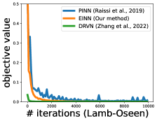
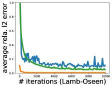
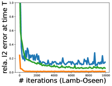
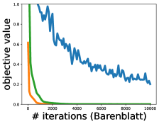
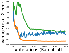
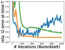
Figure 1: The first row contains results for the 2D NSE and the second row contains the results for the 3D MVE with Coulomb interaction. The first column reports the objective losses, while the second and third columns report the average and last-time-stamp relative $\ell_{2}$ error.

We present the results of our experiments in Figure 1, where the first row contains the result for the Lamb-Oseen vortex (2D NSE) and the second row contains the result for the Barenblatt model (3D MVE). The explicit solutions of these models allow us to assess the quality of the outputs of the included methods. Specifically, given a hypothesis solution $\rho_{t}^{f}$, the ground truth $\bar{\rho}_{t}$ and the interaction kernel $K$, define the relative $\ell_{2}$ error at timestamp $t$ as $Q(t)\overset{\operatorname{def}}{=}\int_{\Omega}{\|K\ast(\rho^{f}_{t}-\bar{\rho}_{t})({\bm{x}})\|}/{\|K\ast\bar{\rho}_{t}({\bm{x}})\|}d{\bm{x}}$, where $\Omega$ is some domain where $\rho_{t}$ has non-zero density. We are particularly interested in the quality of the convolution term $K\ast\rho^{f}_{t}$ since it has physical meanings. In the Biot-Savart kernel case, it is the velocity of the fluid, while in the Coulomb case, it is the Coulomb field. We set $\Omega$ to be $[-2,2]^{2}$ for the Lamb-Oseen vortex and to $[-0.1,0.1]^{3}$ for the Barenblatt model. For both models, we take $\nu=0.1$, $t_{0}=0.1$, and $T=1$. The neural network that we use is an MLP with $7$ hidden layers, each of which has 20 neurons.
From the first column of Figure 1, we see that the objective loss of all methods has substantially reduced over a training period of 10000 iterations. This excludes the possibility that a baseline has worse performance because the NN is not well-trained, and hence the quality of the solution now solely depends on the efficacy of the method. From the second and third columns, we see that the proposed EINN method significantly outperforms the other two methods in terms of the time-average relative $\ell_{2}$ error, i.e. $\frac{1}{T}\int_{0}^{T}Q(t)dt$ and the relative $\ell_{2}$ error at the last time stamp $Q(T)$. This shows the advantage of our method.

Conclusion

By employing entropy dissipation of the MVE, we design a potential function for a hypothesis velocity field such that it controls the KL divergence between the corresponding hypothesis solution and the ground truth, for any time stamp within the period of interest. Built on this potential, we proposed the EINN method for MVEs with NN and derived the detailed computation method of the stochastic gradient, using the classic adjoint method. Through empirical studies on examples of the 2D NSE and the 3D MVE with Coulomb interactions, we show the significant advantage of the proposed method, when compared with two SOTA NN based MVE solvers.

Appendix A Classical Methods for Solving MVEs

Solving partial differential equations (PDEs) is a key aspect of scientific research, with a wealth of literature in the field [Evans, 2022]. For the interest of this paper, we will only consider the methods that can be used to solve the MVE under consideration.

Categorize PDE solvers via solution representation.

To better understand the benefits of neural network (NN) based PDE solvers and to compare our approach with others, we categorize the literature based on the representation of the solution to the PDE. These representations can be roughly grouped into four categories:

• 1. Discretization-based representation: The solution to the PDE is represented as discrete function values at grid points, finite-size cells, or finite-element meshes.

• 2. Representation as a combination of basis functions: The solution to the PDE is approximated as a sum of basis functions, e.g. Fourier series, Legendre polynomials, or Chebyshev polynomials.

• 3. Representation using a collection of particles: The solution to the PDE is represented as a collection of particles, each described by its weight, position, and other relevant information.

• 4. NN-based representation: NNs offer many strategies for representing the solution to the PDE, such as using the NN directly to represent the solution, using normalizing flow or GAN-based parameterization to ensure the non-negativity and conservation of mass of the solution or using the NN to parameterize the underlying dynamics of the PDE, such as the time-varying velocity field that drives the evolution of the system.

The drawback of the first three strategies is that a sparse representation leads to reduced solution accuracy, while a dense representation results in increased computational and memory cost. NNs, as powerful function approximation tools, are expected to surpass these strategies by being able to handle higher-dimensional, less regular, and more complicated systems [Weinan et al., 2021].

Given a representation strategy of the solution, an effective solver must exploit the underlying properties of the system to find the best candidate solution. Three-= notable properties that are utilized to design solvers are

1. the PDE definition or weak formulation of the system,

2. the SDE interpretation of the system,

3. the variational interpretation, particularly the Wasserstein gradient flow interpretation.

These properties are combined with the solution representations mentioned earlier to form different methods. For example, the Finite Difference method [Smith et al., 1985], Finite Volume method [Moukalled et al., 2016], and Finite Element method [Johnson, 2012] represent the solution of partial differential equations (PDEs) by discretizing the solution and utilize the property (A), at least in their original form. On the other hand, recent work by Carrillo et al. [2022] solves PDEs admitting a Wasserstein gradient flow structure using the classic JKO scheme [Jordan et al., 1998], which is based on the property (C), and the solution is also represented via discretization. The Spectral method [Shen et al., 2011] is a class of methods that exploits property (A) by representing the solution as a combination of basis functions. The Random Vortex Method [Long, 1988] is a highly successful method for solving the vorticity formulation of the 2D Navier-Stokes equation by exploiting property (C) and representing the solution with particles. The Blob method from Carrillo et al. [2019] is another particle-based method for solving PDEs that describe diffusion processes, which also exploits property (C).

Appendix B Comparison with Neural Operator

We thank the anonymous reviewers for pointing out the interesting research direction of neural operators [Xiao et al., 2023, Gupta et al., 2021, Li et al., 2020b, Kovachki et al., 2021, Li et al., 2020a]. However, to highlight the major difference between EINN and the approach of the Neural Operator, it’s worth noting that they consider completely different problem settings: EINN requires no pre-existing data and the goal is to obtain the solution to a PDE by solely exploiting the structure of the equation itself. In contrast, the neural operator approach is data-driven, i.e. it relies on the existence of configuration-solution pairs. Here, by configuration-solution pairs, we mean the correspondence between some configurations that determine the PDE, e.g. the initial condition or the viscosity parameter in the fluid dynamics problems, and the pre-existing solution to the PDE given the aforementioned configurations. Consequently, the neural operator approach is more like a regression problem where a neural network is trained to learn the abstract map between the configuration and the solution. In contrast, EINN is more like a numerical PDE solver.

Consequently, EINN and the approach of neural operator are two related but quite distinct research directions. They are related in the sense that EINN can provide the data (configuration-solution pairs) required by the neural operator approach. They are distinct since EINN requires no data a priori, while the neural operator approach is built on the supervised learning paradigm.

Appendix C More Details on the Experiments

C.1 Implementations of Baselines

Objectives of PINN

• For the vorticity equation of the 2D Navier-Stokes equation, let ${\bm{u}}:[0,T]\times{\mathbb{R}}^{2}\rightarrow{\mathbb{R}}^{2}$ be the velocity field (this should not be confused with the velocity field of the continuity equation) such that $\nabla\cdot{\bm{u}}=0$, i.e. ${\bm{u}}$ is divergence-free, and let $\omega=\nabla\times{\bm{u}}\in{\mathbb{R}}$ be the vorticity. We have

  $$\frac{\partial\omega}{\partial t}+\nabla\cdot\left(\omega{\bm{u}}\right)= \ \nu\Delta\omega,$$ (24)

  $$\omega= \ \nabla\times{\bm{u}}.$$ (25)

  We use this form to construct the objective for the PINN method

  $$\int_{0}^{T}\|\frac{\partial\omega}{\partial t}+\nabla\cdot\left(\omega{\bm{u}}\right)-\nu\Delta\omega\|_{{\mathcal{L}}(\Omega)^{2}}^{2}+\|\omega-\nabla\times{\bm{u}}\|_{{\mathcal{L}}(\Omega)^{2}}dt,$$ (26)

  where ${\mathcal{L}}^{2}(\Omega)$ denotes the functional ${\mathcal{L}}^{2}$ norm on the domain $\Omega=[-2,2]^{2}$.

• For the MVE with Coulomb interaction, let $g$ be the Coulomb potential defined in equation 3. We have that $\psi=g\ast\rho$ is the solution to the Poisson equation $\Delta\psi=-\rho$ and $K*\rho=-\nabla\psi$. We have

  $$\frac{\partial\rho}{\partial t}+\nabla\cdot\left(\rho\cdot(-\nabla\psi)\right)= \ \nu\Delta\rho$$ (27)

  $$\Delta\psi= \ -\rho.$$ (28)

  Expand the the divergence to obtain

  $$\frac{\partial\rho}{\partial t}+\nabla\rho\cdot(-\nabla\psi)+\rho\cdot(-\Delta\psi)= \ \nu\Delta\rho$$ (29)

  $$\Delta\psi= \ -\rho.$$ (30)

  Now plug in the $\Delta\psi=-\rho$ to arrive at the following equivalent form

  $$\frac{\partial\rho}{\partial t}+\nabla\rho\cdot-\nabla\psi+\rho^{2}= \ \nu\Delta\rho$$ (31)

  $$\Delta\psi= \ -\rho.$$ (32)

  We use this form to construct the objective for the PINN method.

  $$\int_{0}^{T}\|\frac{\partial\rho}{\partial t}+\nabla\rho\cdot-\nabla\psi+\rho^{2}-\nu\Delta\rho\|_{{\mathcal{L}}^{2}(\Omega)}^{2}+\|\Delta\psi+\rho\|_{{\mathcal{L}}^{2}}^{2},$$ (33)

  where ${\mathcal{L}}^{2}(\Omega)$ denotes the functional ${\mathcal{L}}^{2}$ norm on the domain $\Omega=[-1,1]^{2}$.

DRVN

In the original paper [Zhang et al., 2022], only the Biot-Savart kernel is concerned. We extend the DRVN method to the Coulomb case by setting $K$ to be the kernel defined in equation 3.

C.2 Examples with an Explicit Solution

In this section, we verify the explicit solutions discussed in the experiment section.

Lamb-Oseen Vortex on the whole domain ${\mathbb{R}}^{2}$.

Recall that we consider the 2D Navier-Stokes equation (the MVE with the Biot-Savart interaction kernel (4)). The Lamb-Oseen Vortex model states that, if $\rho_{0}=\mathcal{N}(0,\sqrt{2\nu t_{0}}{\bm{I}}_{2})$ for some $t_{0}\geq 0$, then we have $\rho_{t}({\bm{x}})=\mathcal{N}(0,\sqrt{2\nu(t+t_{0})}{\bm{I}}_{2})$.

To verify this, define ${\bm{u}}_{t}({\bm{x}})=\frac{1}{\sqrt{\nu(t+t_{0})}}{\bm{v}}(\frac{{\bm{x}}}{\sqrt{\nu(t+t_{0})}})$, where

$${\bm{v}}({\bm{x}})=\frac{1}{2\pi}\frac{{\bm{x}}^{\perp}}{\|{\bm{x}}\|^{2}}\left(1-\exp(-\frac{1}{4}\|{\bm{x}}\|^{2})\right).$$ (34)

One can easily check that $\nabla\cdot{\bm{u}}_{t}\equiv 0$ and hence there exists a function $\psi_{t}$ such that $\nabla^{\perp}\psi_{t}=-{\bm{u}}_{t}$, where $\nabla^{\perp}$ denotes the perpendicular gradient, defined as $\nabla^{\perp}=(-\partial_{{\bm{x}}_{2}},\partial_{{\bm{x}}_{2}})$, and $\psi_{t}$ is called the stream function in the literature of fluid dynamics. Moreover, one can verify that $\nabla\times{\bm{u}}_{t}=\rho_{t}$ where $\nabla\times$ denotes the curl of a 2D velocity field, defined as $\nabla\times{\bm{u}}({\bm{x}})=\partial{\bm{u}}_{2}/\partial{\bm{x}}_{1}-\partial{\bm{u}}_{1}/\partial{\bm{x}}_{2}$. Together we have

$$\Delta\psi_{t}=-\rho_{t},$$ (35)

i.e., the stream function $\psi_{t}$ is the solution to the 2D Poisson equation with a source term $\rho_{t}$.

Under the boundary condition that $\psi_{t}({\bm{x}})\rightarrow 0$ for $\|{\bm{x}}\|\rightarrow\infty$, we can express $\psi_{t}$ via the unique Green function $G({\bm{x}})=\frac{1}{2\pi}\ln\|{\bm{x}}\|$ as

$$\psi_{t}({\bm{x}})=G\ast\rho_{t}=\frac{1}{2\pi}\int\ln\|{\bm{x}}-{\bm{y}}\|\rho_{t}({\bm{y}})d{\bm{y}}.$$ (36)

Consequently, by taking the perpendicular gradient, we obtain

$${\bm{u}}_{t}=\nabla^{\perp}\psi_{t}=\frac{1}{2\pi}\int\frac{({\bm{x}}-{\bm{y}})^{\perp}}{\|{\bm{x}}-{\bm{y}}\|^{2}}\rho_{t}({\bm{y}})d{\bm{y}}=K\ast\rho_{t}.$$ (37)

Finally, by plugging the expressions of $\rho_{t}$ and ${\bm{u}}_{t}=K\ast\rho_{t}$ in the MVE (2), we verified the Lamb-Oseen vortex.

Barenblatt solutions for the MVE with Coulomb Interaction.

Recall that we consider the MVE with the Coulomb interaction kernel (3) for $d=3$ and set the diffusion coefficient $\nu=0$, i.e.

$$\frac{\partial\rho_{t}}{\partial t}+\nabla\cdot\left(\rho_{t}\cdot-\nabla\psi_{t}\right)=0$$ (38)

where $\psi_{t}$ is the solution to the Poisson equation $\Delta\psi_{t}=-\rho_{t}$. The Barenblatt solution of the above MVE is stated as follows: If $\rho_{0}=\mathrm{Uniform}[\|{\bm{x}}\|\leq(\frac{3}{4\pi}t_{0})^{1/3}]$ for some $t_{0}\geq 0$, then we have

$$\rho_{t}=\mathrm{Uniform}[\|{\bm{x}}\|\leq(\frac{3}{4\pi}(t+t_{0}))^{1/3}]$$ (39)

We now verify this solution.

Recall that the volume of a three dimensional Euclidean ball with radius $R$ is $\frac{4\pi}{3}R^{3}$. Hence we can write the density function as $\rho_{t}(x)=\frac{1}{t+t_{0}}\chi_{\|{\bm{x}}\|\leq(\frac{3}{4\pi}(t+t_{0}))^{1/3}}$, where $\chi_{\mathbb{X}}$ is a function that takes value $1$ for ${\bm{x}}\in{\mathbb{X}}$ and takes value $0$ for ${\bm{x}}\notin{\mathbb{X}}$. Take

$$\psi_{t}({\bm{x}})=\begin{cases}\frac{2(\frac{3}{4\pi}(t+t_{0}))^{2/3}-\|{\bm{x}}\|^{2}}{6(t+t_{0})},&\|{\bm{x}}\|\leq(\frac{3}{4\pi}(t+t_{0}))^{1/3},\\ \frac{1}{8\pi\|{\bm{x}}\|},&\|{\bm{x}}\|>(\frac{3}{4\pi}(t+t_{0}))^{1/3}.\end{cases}$$ (40)

It can be verified that the Poisson equation $\Delta\psi_{t}=-\rho_{t}$ holds (note that $\Delta\|{\bm{x}}\|^{-1}=0$, i.e. $\|{\bm{x}}\|^{-1}$ is a harmonic function for $d=3$). Consequently, for a fixed time stamp $t$ and any $\|{\bm{x}}\|\leq(\frac{3}{4\pi}(t+t_{0}))^{1/3}$ we have

$$\frac{\partial\rho_{t}}{\partial t}({\bm{x}})+\nabla\cdot\left(\rho_{t}({\bm{x}})\cdot-\nabla\psi_{t}({\bm{x}})\right)=-\frac{1}{(t+t_{0})^{2}}+\frac{1}{(t+t_{0})^{2}}=0,$$ (41)

which verifies this solution.

Appendix D Adjoint Method

Consider the ODE system

$$\dot{s}(t)= \ \psi(s(t),t,\theta)$$

$$s(0)= \ s_{0},$$

and the objective loss

$$\ell(\theta)=\int_{0}^{T}g(s(t),t,\theta)\mathrm{d}t.$$ (42)

The following proposition computes the gradient of $\ell$ w.r.t. $\theta$. We omit the parameters of the functions for succinctness. We note that all the functions in the integrands should be evaluated at the corresponding time stamp $t$, e.g. $b^{\top}\frac{\partial h}{\partial\theta}\mathrm{d}t$ abbreviates for $b(t)^{\top}\frac{\partial}{\partial\theta}h(\xi(t),x(t),t,\theta)\mathrm{d}t$.

Proposition 1.

$$\frac{\mathrm{d}\ell}{\mathrm{d}\theta}=\int_{0}^{T}a^{\top}\frac{\partial\psi}{\partial\theta}+\frac{\partial g}{\partial\theta}\mathrm{d}t.$$ (43)

where $a(t)$ is solution to the following final value problems

$$\dot{a}^{\top}+a^{\top}\frac{\partial\psi}{\partial s}+\frac{\partial g}{\partial s}=0,a(T)=0,$$ (44)

Proof.

Let us define the Lagrange multiplier function (or the adjoint state) $a(t)$ dual to $s(t)$. Moreover, let $L$ be an augmented loss function of the form

$$L=\ell-\int_{0}^{T}a^{\top}(\dot{s}-\psi)\mathrm{d}t.$$ (45)

Since we have $\dot{s}(t)=\psi(s(t),t,\theta)$ by construction, the integral term in $L$ is always null and $a$ can be freely assigned while maintaining $\mathrm{d}L/\mathrm{d}\theta=\mathrm{d}\ell/\mathrm{d}\theta$. Using integral by part, we have

$$\int_{0}^{T}a^{\top}\dot{s}\ \mathrm{d}t=a(t)^{\top}s(t)|_{0}^{T}-\int_{0}^{T}s^{\top}\dot{a}\ \mathrm{d}t.$$ (46)

We obtain

$$L=-a(t)^{\top}s(t)|_{0}^{T}+\int_{0}^{T}\dot{a}^{\top}s+a^{\top}\psi+g\ \mathrm{d}t.$$ (47)

Now we compute the gradient of $L$ w.r.t. $\theta$ as

$$\frac{\mathrm{d}\ell}{\mathrm{d}\theta}=\frac{\mathrm{d}L}{\mathrm{d}\theta}=-a(T)^{\top}\frac{\mathrm{d}x(T)}{\mathrm{d}\theta}+\int_{0}^{T}\dot{a}^{\top}\frac{\mathrm{d}s}{\mathrm{d}\theta}+a^{\top}\left(\frac{\partial\psi}{\partial\theta}+\frac{\partial\psi}{\partial s}\frac{\mathrm{d}s}{\mathrm{d}\theta}\right)\mathrm{d}t+\int_{0}^{T}\frac{\partial g}{\partial s}\frac{\mathrm{d}s}{\mathrm{d}\theta}+\frac{\partial g}{\partial\theta}\mathrm{d}t,$$

which by rearranging terms yields to

$$\frac{\mathrm{d}\ell}{\mathrm{d}\theta}=\frac{\mathrm{d}L}{\mathrm{d}\theta}=-a(T)^{\top}\frac{\mathrm{d}x(T)}{\mathrm{d}\theta}+\int_{0}^{T}a^{\top}\frac{\partial\psi}{\partial\theta}+\frac{\partial g}{\partial\theta}\mathrm{d}t+\int_{0}^{T}\left(\dot{a}^{\top}+a^{\top}\frac{\partial\psi}{\partial s}+\frac{\partial g}{\partial s}\right)\frac{\mathrm{d}s}{\mathrm{d}\theta}\mathrm{d}t.$$

Now by taking $a$ satisfying the final value problems

$$\dot{a}^{\top}+a^{\top}\frac{\partial\psi}{\partial s}+\frac{\partial g}{\partial s}=0,a(T)=0,$$ (48)

we derive the result

$$\frac{\mathrm{d}\ell}{\mathrm{d}\theta}=\int_{0}^{T}a^{\top}\frac{\partial\psi}{\partial\theta}+\frac{\partial g}{\partial\theta}\mathrm{d}t.$$ (49)

D.1 Writing the Trajectory-wise Loss (15) in an ODE-constrained form

We are now ready to write $R(f_{\theta};{\bm{x}}_{0})$ in an ODE-constrained form. Define the state ${\bm{s}}(t)$, the initial condition ${\bm{s}}_{0}$ and the transition function $\psi$ as follows: Let

$${\bm{s}}(t)=\left[{\bm{x}}(t),\xi(t),\{{\bm{y}}_{i}(t)\}_{i=1}^{N},\{\zeta_{i}(t)\}_{i=1}^{N}\right],$$ (50)

with $\xi(t)=\nabla\log\rho_{t}^{f}({\bm{x}}(t))$ and $\zeta_{i}(t)=\nabla\log\rho_{t}^{f}({\bm{y}}_{i}(t))$. Take the initial condition

$${\bm{s}}_{0}=\left[{\bm{x}}_{0},\xi_{0},\{{\bm{y}}_{i}(0)\}_{i=1}^{N},\{\zeta_{i}(0)\}_{i=1}^{N}\right]$$ (51)

with $\xi_{0}=\nabla\log\bar{\rho}_{0}({\bm{x}}_{0})$, $\zeta_{i}(0)=\nabla\log\bar{\rho}_{0}({\bm{y}}_{i}(0))$, and ${\bm{y}}_{i}(0)\stackrel{{\scriptstyle iid}}{{\sim}}\bar{\rho}_{0}$; and define the function

$$\psi(t,s(t);\theta)=[f_{t}({\bm{x}}(t);\theta),\ h_{t}({\bm{x}}(t),\xi(t);\theta),\ \{f_{t}({\bm{y}}_{i}(t);\theta)\}_{i=1}^{N},\ \{h_{t}({\bm{y}}_{i}(t),\zeta_{i}(t);\theta)\}_{i=1}^{N}],$$ (52)

where $h({\bm{a}},{\bm{b}};\theta)=-\nabla\left(\,\mathrm{div}f_{t}({\bm{a}};\theta)\right)-{\mathcal{J}}^{\top}_{f_{t}}({\bm{a}};\theta){\bm{b}}$ (derived from equation 18). Finally, define

$$g(t,{\bm{s}}(t);\theta)=\|f(t,{\bm{x}}(t);\theta)-\left(-\nabla V({\bm{x}}(t))+E(t,{\bm{s}}(t))-\nu\xi(t)\right)\|^{2},$$ (53)

where the estimator $E(t,{\bm{s}})$ of the convolution term is defined as

$$E(t,{\bm{s}}(t))=\begin{cases}\frac{1}{N}\sum_{i=1}^{N}K_{c}({\bm{x}}(t)-{\bm{y}}_{i}(t))&\text{the Coulomb case},\\ \frac{1}{N}\sum_{i=1}^{N}U({\bm{x}}-{\bm{y}}_{i}(t))\zeta_{i}(t)&\text{the Biot-Savart case}.\end{cases}$$ (54)

We recall the definition of $U$ in equation 21 and the definition of $K_{c}$ in equation 19. ∎

Appendix E Detailed Proofs

Proof of Lemma 1.

Recall the McKean-Vlasov equation 6 and the continuity equation 10. We simply write that $\rho_{t}=\rho_{t}^{f}$ and omit the integration domain $\mathcal{X}$. Then

$$\begin{split}&\frac{\mathrm{d}}{\mathrm{d}t}\int\rho_{t}\log\frac{\rho_{t}}{\bar{\rho}_{t}}=\int\partial_{t}\rho_{t}\log\frac{\rho_{t}}{\bar{\rho}_{t}}+\int\rho_{t}\partial_{t}\log\rho_{t}-\int\rho_{t}\partial_{t}\log\bar{\rho}_{t}\\ &=-\int\,\mathrm{div}\Big{(}\rho_{t}\Big{(}\Big{[}-\nabla V(x)+K*\rho_{t}-\nu\nabla\log\rho_{t}\Big{]}+\delta_{t}\Big{)}\Big{)}\log\frac{\rho_{t}}{\bar{\rho}_{t}}\\ &+\int\frac{\rho_{t}}{\bar{\rho}_{t}}\,\mathrm{div}\Big{(}\bar{\rho}_{t}\Big{(}-\nabla V(x)+K*\bar{\rho}_{t}-\nu\nabla\log\bar{\rho}_{t}\Big{)}\Big{)},\end{split}$$

where we note that $\int\rho_{t}\partial_{t}\log\rho_{t}=\int\partial_{t}\rho_{t}=0$ since the total mass is preserved over time. By integration by parts, one has

$$\begin{split}&\frac{\mathrm{d}}{\mathrm{d}t}\int\rho_{t}\log\frac{\rho_{t}}{\bar{\rho}_{t}}=I_{1}+I_{2}+I_{3}+\int\rho_{t}\delta_{t}\cdot\nabla\log\frac{\rho_{t}}{\bar{\rho}_{t}},\end{split}$$

where $I_{1},I_{2},I_{3}$ denote the linear, nonlinear interaction, and diffusion parts separately. More precisely, by integration by parts,

$$\begin{split}I_{1}&=\int\,\mathrm{div}(\rho_{t}\nabla V(x))\log\frac{\rho_{t}}{\bar{\rho}_{t}}-\int\frac{\rho_{t}}{\bar{\rho}_{t}}\,\mathrm{div}(\bar{\rho}_{t}\nabla V(x))\\ &=-\int\rho_{t}\nabla V(x)\cdot\nabla\log\frac{\rho_{t}}{\bar{\rho}_{t}}+\int\bar{\rho}_{t}\nabla\frac{\rho_{t}}{\bar{\rho}_{t}}\cdot\nabla V(x)=0.\end{split}$$

And

$$\begin{split}I_{2}&=-\int\,\mathrm{div}(\rho_{t}K*\rho_{t})\log\frac{\rho_{t}}{\bar{\rho}_{t}}+\int\frac{\rho_{t}}{\bar{\rho}_{t}}\,\mathrm{div}(\bar{\rho}_{t}K*\bar{\rho}_{t})\\ &=\int\rho_{t}K*\rho_{t}\nabla\log\frac{\rho_{t}}{\bar{\rho}_{t}}-\int\bar{\rho}_{t}K*\bar{\rho}_{t}\cdot\nabla\frac{\rho_{t}}{\bar{\rho}_{t}}\\ &=\int\rho_{t}\nabla\log\frac{\rho_{t}}{\bar{\rho}_{t}}\cdot K*(\rho_{t}-\bar{\rho}_{t}).\end{split}$$

Given that the kernel $K$ is divergence free, that is $\,\mathrm{div}K=0$, one further has

$$\begin{split}I_{2}&=-\int\rho_{t}\nabla\log\bar{\rho}_{t}\cdot K*(\rho_{t}-\bar{\rho}_{t})+\int\nabla\rho_{t}\cdot K*(\rho_{t}-\bar{\rho}_{t})\\ &=-\int\rho_{t}\nabla\log\bar{\rho}_{t}\cdot K*(\rho_{t}-\bar{\rho}_{t}).\end{split}$$ (55)

Note that this modification will be used in the proof in the 2D Navier-Stokes case. Finally, all diffusion terms sum up to $I_{3}$ which can be further simplified as

$$\begin{split}I_{3}&=\nu\int\,\mathrm{div}(\rho_{t}\nabla\log\rho_{t})\log\frac{\rho_{t}}{\bar{\rho}_{t}}-\nu\int\frac{\rho_{t}}{\bar{\rho}_{t}}\,\mathrm{div}(\bar{\rho}_{t}\nabla\log\bar{\rho}_{t})\\ &=-\nu\int\rho_{t}\nabla\log\rho_{t}\cdot\nabla\log\frac{\rho_{t}}{\bar{\rho}_{t}}+\nu\int\bar{\rho}_{t}\nabla\log\bar{\rho}_{t}\cdot\nabla\frac{\rho_{t}}{\bar{\rho}_{t}}\\ &=-\nu\int\rho_{t}|\nabla\log\frac{\rho_{t}}{\bar{\rho}_{t}}|^{2}.\end{split}$$

We thus complete the proof of Lemma 1.

∎

Proof of Lemma 2.

Recall that $K=-\nabla g$. For simplicity, we write that $\rho_{t}=\rho_{t}^{f}$. Then

$$\begin{split}&\frac{\mathrm{d}}{\mathrm{d}t}F(\rho_{t},\bar{\rho}_{t})=\frac{\mathrm{d}}{\mathrm{d}t}\frac{1}{2}\int_{\mathcal{X}^{2}}g(x-y)\mathrm{d}(\rho_{t}-\bar{\rho}_{t})^{\otimes 2}(x,y)\\ &=\int_{\mathcal{X}}g*(\rho_{t}-\bar{\rho}_{t})(x)\big{(}\partial_{t}\rho_{t}(x)-\partial_{t}\bar{\rho}_{t}(x)\Big{)}\mathrm{d}x\\ &=\int g*(\rho_{t}-\bar{\rho}_{t})(x)\,\mathrm{div}\Big{\{}\rho_{t}\Big{(}[\nabla V(x)-K*\rho_{t}+\nu\nabla\log\rho_{t}]-\delta_{t}\Big{)}\\ &\quad\qquad\qquad\qquad\qquad-\bar{\rho}_{t}\Big{(}\nabla V(x)-K*\bar{\rho}_{t}+\nu\log\bar{\rho}_{t}\Big{)}\Big{\}}\\ &=J_{1}+J_{2}+J_{3}+J_{4},\end{split}$$

where $J_{1},J_{2},J_{3},J_{4}$ denote the perturbation term, the linear difference term, the nonlinear difference term, and the diffusion term respectively. The perturbation term $J_{1}$ reads

$$J_{1}=-\int_{\mathcal{X}}g*(\rho_{t}-\bar{\rho}_{t})\,\mathrm{div}(\rho_{t}\delta_{t})=-\int_{\mathcal{X}}\rho_{t}K*(\rho_{t}-\bar{\rho}_{t})\cdot\delta_{t}.$$

By integration by parts, the linear difference term can be written as

$$\begin{split}&J_{2}=\int_{\mathcal{X}}g*(\rho_{t}-\bar{\rho}_{t})\,\mathrm{div}\Big{(}(\rho_{t}-\bar{\rho}_{t})\nabla V\Big{)}=\int_{\mathcal{X}}K*(\rho_{t}-\bar{\rho}_{t})(\rho_{t}-\bar{\rho}_{t})\nabla V\\ &=\frac{1}{2}\int_{\mathcal{X}^{2}}K(x-y)(\nabla V(x)-\nabla V(y))\mathrm{d}(\rho_{t}-\bar{\rho}_{t})^{\otimes 2}(x,y),\end{split}$$

where the last equality is true since $K=-\nabla g$ is an odd function and we do the symmetrization trick, i.e. exchanging the role of $x$ and $y$ to another term and then taking the average.

The nonlinear difference term reads

$$\begin{split}&J_{3}=-\int_{\mathcal{X}}g*(\rho_{t}-\bar{\rho}_{t})\,\mathrm{div}\Big{(}\rho_{t}K*\rho_{t}-\bar{\rho}_{t}K*\bar{\rho}_{t}\Big{)}\\ &=-\int_{\mathcal{X}}K*(\rho_{t}-\bar{\rho}_{t})(\rho_{t}K*(\rho_{t}-\bar{\rho}_{t})-\int_{\mathcal{X}}K*(\rho_{t}-\bar{\rho}_{t})(\rho_{t}-\bar{\rho}_{t})K*\bar{\rho}_{t}\\ &=-\int_{\mathcal{X}}\rho_{t}|K*(\rho_{t}-\bar{\rho}_{t})|^{2}-\frac{1}{2}\int K(x-y)(K*\bar{\rho}_{t}(x)-K*\bar{\rho}_{t}(y))\mathrm{d}(\rho_{t}-\bar{\rho}_{t})^{\otimes 2}(x,y),\end{split}$$

where again in the last term we do the symmetrization.

The diffusion term reads

$$\begin{split}&J_{4}=\nu\int g*(\rho_{t}-\bar{\rho}_{t})\,\mathrm{div}\Big{(}\rho_{t}\nabla\log\rho_{t}-\bar{\rho}_{t}\nabla\log\bar{\rho}_{t}\Big{)}\\ &=\nu\int K*(\rho_{t}-\bar{\rho}_{t})\rho_{t}\nabla\log\frac{\rho_{t}}{\bar{\rho}_{t}}+\nu\int K*(\rho_{t}-\bar{\rho}_{t})(\rho_{t}-\bar{\rho}_{t})\nabla\log\bar{\rho}_{t}\\ &=\nu\int_{\mathcal{X}}\rho_{t}K*(\rho_{t}-\bar{\rho}_{t})\cdot\nabla\log\frac{\rho_{t}}{\bar{\rho}_{t}}\\ &\qquad+\frac{\nu}{2}\int_{\mathcal{X}^{2}}K(x-y)(\nabla\log\bar{\rho}_{t}(x)-\nabla\log\bar{\rho}_{t}(y))\mathrm{d}(\rho_{t}-\bar{\rho}_{t})^{\otimes 2}.\end{split}$$

To sum it up, we prove the thesis.

∎

E.1 Proof of the 2D Navier-Stokes case

Now we proceed to control the growth of the KL divergence $\mathbf{KL}(\rho_{t}^{f}|\bar{\rho}_{t})$ for the 2D Navier-Stokes case. Since the Biot-Savart law is divergence free, by equation 55 in the proof of Lemma 1, one has

$$\frac{\mathrm{d}}{\mathrm{d}t}\int_{\Pi^{d}}\rho_{t}\log\frac{\rho_{t}}{\bar{\rho}_{t}}=-\nu\int_{\Pi^{d}}\rho_{t}|\nabla\log\frac{\rho_{t}}{\bar{\rho}_{t}}|^{2}-\int_{\Pi^{d}}\rho_{t}K*(\rho_{t}-\bar{\rho}_{t})\cdot\nabla\log\bar{\rho}_{t}+\int_{\Pi^{d}}\rho_{t}\delta_{t}\cdot\nabla\log\frac{\rho_{t}}{\bar{\rho}_{t}}.$$ (56)

Recall that we write the kernel $K=(K_{1},\cdots,K_{d})$ and its component $K_{i}=\sum_{j=1}^{d}\partial_{x_{j}}U_{ij}(x)$, where $U=(U_{ij})_{1\leq i,j\leq d}$ is a matrix-valued potential function for instance can be defined as in equation 21. Consequently

$$-\int\rho_{t}K*(\rho_{t}-\bar{\rho}_{t})\cdot\nabla\log\bar{\rho}_{t}=-\sum_{i,j=1}^{d}\int\rho_{t}\partial_{x_{j}}U_{ij}*(\rho_{t}-\bar{\rho}_{t})\partial_{x_{i}}\log\bar{\rho}_{t},$$

which equals to

$$\sum_{i,j=1}^{d}\int U_{ij}*(\rho_{t}-\bar{\rho}_{t})\partial_{x_{j}}\big{(}\frac{\rho_{t}}{\bar{\rho}_{t}}\partial_{x_{i}}\bar{\rho}_{t}\big{)}=A+B$$

by integration by parts, where further

$$A=\sum_{i,j=1}^{d}\int V_{ij}*(\rho_{t}-\bar{\rho}_{t})\,\partial_{x_{i}}\bar{\rho}_{t}\,\partial_{x_{j}}\,\frac{\rho_{t}}{\bar{\rho}_{t}}=\int U*(\rho_{t}-\bar{\rho}_{t}):\nabla\bar{\rho}_{t}\otimes\nabla\frac{\rho_{t}}{\bar{\rho}_{t}},$$

and

$$B=\sum_{i,j=1}^{d}\int\rho_{t}U_{ij}*(\rho_{t}-\bar{\rho}_{t})\frac{\partial_{x_{i}x_{j}}^{2}\bar{\rho}_{t}}{\bar{\rho}_{t}}=\int\rho_{t}U*(\rho_{t}-\bar{\rho}_{t}):\frac{\nabla^{2}\bar{\rho}_{t}}{\bar{\rho}_{t}}.$$

Noticing that $\nabla\frac{\rho_{t}}{\bar{\rho}_{t}}=\frac{\rho_{t}}{\bar{\rho}_{t}}\nabla\log\frac{\rho_{t}}{\bar{\rho}_{t}}$, one estimates $A$ as follows

$$\begin{split}A&=\int\rho_{t}U*(\rho_{t}-\bar{\rho}_{t}):\nabla\log\bar{\rho}_{t}\otimes\nabla\log\frac{\rho_{t}}{\bar{\rho}_{t}}\\ &\leq\frac{\nu}{4}\int\rho_{t}|\nabla\log\frac{\rho_{t}}{\bar{\rho}_{t}}|^{2}+\frac{1}{\nu}\int\rho_{t}|(\nabla\log\bar{\rho}_{t})^{\top}\,U*(\rho-\bar{\rho})|^{2}\\ &\leq\frac{\nu}{4}\int\rho_{t}|\nabla\log\frac{\rho_{t}}{\bar{\rho}_{t}}|^{2}+\frac{1}{\nu}\|U\|_{L^{\infty}}^{2}\|\nabla\log\bar{\rho}_{t}\|_{L^{\infty}}^{2}\|\rho_{t}-\bar{\rho}_{t}\|_{L^{1}}^{2},\end{split}$$

and again by Csiszár–Kullback–Pinsker inequality, one has that

$$A\leq\frac{\nu}{4}\int\rho_{t}|\nabla\log\frac{\rho_{t}}{\bar{\rho}_{t}}|^{2}+\frac{2}{\nu}\|U\|_{L^{\infty}}^{2}\|\nabla\log\bar{\rho}_{t}\|_{L^{\infty}}^{2}\int\rho_{t}\log\frac{\rho_{t}}{\bar{\rho}_{t}}.$$

Now it only remains to control $B$. Recall the following famous Gibbs inequality

Lemma 4 (Gibbs inequality).

For any parameter $\eta>0$, and probability measures $\rho,\bar{\rho}\in\mathcal{P}(\mathcal{X})\cap L^{1}(\mathcal{X})$, and $\phi$ a real-valued function defined on $\mathcal{X}$, one has the following change of reference measure inequality

$$\int_{\mathcal{X}}\rho(x)\phi(x)\mathrm{d}x\leq\frac{1}{\eta}\Big{(}\int_{\mathcal{X}}\rho(x)\log\frac{\rho(x)}{\bar{\rho}(x)}\mathrm{d}x+\log\int_{\mathcal{X}}\bar{\rho}(x)\exp(\eta\phi(x))\mathrm{d}x\Big{)}.$$

The proof of this inequality can be found in section 13.1 in [Erdős and Yau, 2017].

To control $B$, we write that $\phi=U*(\rho_{t}-\bar{\rho}_{t}):\frac{\nabla^{2}\bar{\rho}_{t}}{\bar{\rho}_{t}}$ and thus $B=\int\rho_{t}\phi$. We choose a positive parameter $\eta>0$ such that

$$\frac{1}{\eta}=2\|U\|_{L^{\infty}}\Big{\|}\frac{\nabla^{2}\bar{\rho}_{t}}{\bar{\rho}_{t}}\Big{\|}_{L^{\infty}}.$$

Now we apply Lemma 4 to obtain that

$$B=\int\rho_{t}\phi\leq\frac{1}{\eta}\left(\int\rho_{t}\log\frac{\rho_{t}}{\bar{\rho}_{t}}+\log\int\bar{\rho}_{t}\exp(\eta\phi)\right).$$

Note that $\eta>0$ is chosen so small such that

$$\begin{split}\eta\|\phi\|_{L^{\infty}}&\leq\frac{1}{2\|U\|_{L^{\infty}}\Big{\|}\frac{\nabla^{2}\bar{\rho}_{t}}{\bar{\rho}_{t}}\Big{\|}_{L^{\infty}}}\|U\|_{L^{\infty}}\|\rho_{t}-\bar{\rho}_{t}\|_{L^{1}}\Big{\|}\frac{\nabla^{2}\bar{\rho}_{t}}{\bar{\rho}_{t}}\Big{\|}_{L^{\infty}}\\ &\leq\frac{1}{2}\|\rho_{t}-\bar{\rho}_{t}\|_{L^{1}}\leq 1,\end{split}$$

since for two probability densities it always holds $\|\rho_{t}-\bar{\rho}_{t}\|_{L^{1}}\leq 2$. Consequently, applying the inequality $\exp(x)\leq 1+x+\frac{e}{2}x^{2}$ for $|x|\leq 1$, we have

$$\int\bar{\rho}_{t}\exp(\eta\phi)\leq\int\bar{\rho}_{t}\left(1+\eta\phi+\frac{e}{2}\eta^{2}\phi^{2}\right)\leq 1+0+\frac{e}{2}\Big{(}\frac{1}{2}\|\rho_{t}-\bar{\rho}_{t}\|_{L^{1}}\Big{)}^{2}\leq 1+\frac{e}{4}\mathbf{KL}(\rho_{t}|\bar{\rho}_{t}),$$

where

$$\int\bar{\rho}_{t}\phi=\int U*(\rho_{t}-\bar{\rho}_{t}):\nabla^{2}\bar{\rho}_{t}=\int\sum_{i,j=1}^{d}\partial_{x_{i}x_{j}}U*(\rho_{t}-\bar{\rho}_{t})\bar{\rho}_{t}=\int\,\mathrm{div}K*(\rho_{t}-\bar{\rho}_{t})\bar{\rho}_{t}=0,$$

since $\,\mathrm{div}K=0$.

To sum it up, in particular since $\log(1+x)\leq x$ for $x>0$, one has

$$B\leq\frac{1}{\eta}\Big{(}1+\frac{e}{4}\Big{)}\mathbf{KL}(\rho_{t}|\bar{\rho}_{t})\leq 4\|U\|_{L^{\infty}}\Big{\|}\frac{\nabla^{2}\bar{\rho}_{t}}{\bar{\rho}_{t}}\Big{\|}_{L^{\infty}}\mathbf{KL}(\rho_{t}|\bar{\rho}_{t}).$$

Combining equation 56, the estimates for $A$ and $B$, one has

$$\begin{split}&\frac{\mathrm{d}}{\mathrm{d}t}\int\rho_{t}\log\frac{\rho_{t}}{\bar{\rho}_{t}}\leq-\frac{3\nu}{4}\int\rho_{t}|\nabla\log\frac{\rho_{t}}{\bar{\rho}_{t}}|^{2}+M(t)\int\rho_{t}\log\frac{\rho_{t}}{\bar{\rho}_{t}}+\int\rho_{t}\delta_{t}\cdot\nabla\log\frac{\rho_{t}}{\bar{\rho}_{t}}\\ &\leq-\frac{\nu}{2}\int\rho_{t}|\nabla\log\frac{\rho_{t}}{\bar{\rho}_{t}}|^{2}+M(t)\int\rho_{t}\log\frac{\rho_{t}}{\bar{\rho}_{t}}+\frac{1}{\nu}\int\rho_{t}|\delta_{t}|^{2}\end{split}$$ (57)

where

$$M(t)=\frac{2}{\nu}\|U\|_{L^{\infty}}^{2}\|\nabla\log\bar{\rho}_{t}\|_{L^{\infty}}^{2}+4\|U\|_{L^{\infty}}\Big{\|}\frac{\nabla^{2}\bar{\rho}_{t}}{\bar{\rho}_{t}}\Big{\|}_{L^{\infty}}=M(t;\nu,U,\bar{\rho}_{t}).$$

Since the matrix-valued potential function $U$ is bounded ($\|U({\bm{x}})\|_{op}\leq 1/4$ when $U$ takse the form (21)), and under suitable assumptions for the initial data $\bar{\rho}_{0}$ (for instance $\bar{\rho}_{0}\in C^{3}$ and there exists $c>1$ s.t. $\frac{1}{c}\leq\bar{\rho}\leq c$), one can obtain $\sup_{t\in[0,T]}M(t)\leq M<\infty$. We recall Theorem 2 in [Guillin et al., 2021] as below for completeness.

Theorem 5.

Given the initial data $\bar{\rho}_{0}\in C^{\infty}(\Pi^{d})$, such that there exists $c>1$, $\frac{1}{c}\leq\bar{\rho}_{0}\leq c$. Then the vorticity formulation of the 2D Navier-Stokes equation

$$\partial_{t}\bar{\rho}_{t}+\,\mathrm{div}(\bar{\rho}_{t}K*\bar{\rho}_{t})=\nu\Delta\bar{\rho}_{t},\quad\bar{\rho}(0,x)=\bar{\rho}_{0}(x),$$

has a unique bounded solution $\bar{\rho}(t,x)\in C^{\infty}([0,\infty)\times\Pi^{d})$, and for any $t>0$, for any $x\in\Pi^{d}$, it holds that $\frac{1}{c}\leq\bar{\rho}(t,x)\leq c$.

Finally, we simplify equation 57 to obtain that

$$\frac{\mathrm{d}}{\mathrm{d}t}\int\rho_{t}\log\frac{\rho_{t}}{\bar{\rho}_{t}}\leq M\int\rho_{t}\log\frac{\rho_{t}}{\bar{\rho}_{t}}+\frac{1}{\nu}\int\rho_{t}|\delta_{t}|^{2},$$

where $M=\sup_{t\in[0,T]}M(t;\nu,U,\bar{\rho}_{t})<\infty$. By Gronwall inequality, one finally obtains that

$$\sup_{t\in[0,T]}\int_{\Pi^{d}}\rho_{t}\log\frac{\rho_{t}}{\bar{\rho}_{t}}\mathrm{d}x\leq\frac{1}{\nu}\exp(MT)R(\theta).$$

As noted in [Guillin et al., 2021],in particular Corollary 2 there, one can improve the above time-dependent estimate ($\exp(MT)$) to uniform-in-time estimate by using Logarithmic Sobolev inequality. Indeed, given that $\frac{1}{c}\leq\bar{\rho}_{t}\leq c$, one has that

$$\int_{\Pi^{d}}\rho_{t}\log\frac{\rho_{t}}{\bar{\rho}_{t}}\mathrm{d}x\leq\frac{c^{2}}{8\pi^{2}}\int_{\Pi^{d}}\rho_{t}|\nabla_{x}\log\frac{\rho_{t}}{\bar{\rho}_{t}}|^{2}\mathrm{d}x.$$ (58)

Combining equation 58 and equation 57, one obtains that

$$\frac{\mathrm{d}}{\mathrm{d}t}\mathbf{KL}(\rho_{t}|\bar{\rho}_{t})\leq\Big{(}M(t)-\frac{4\pi^{2}\nu}{c^{2}}\Big{)}\mathbf{KL}(\rho_{t}|\bar{\rho}_{t})+\frac{1}{\nu}\int\rho_{t}|\delta_{t}|^{2}.$$

Multiplying the factor $\exp(\frac{4\pi^{2}\nu}{c^{2}}t-\int_{0}^{t}M(s)\mathrm{d}s)$ and noting in particular $\mathbf{KL}(\rho_{0}|\bar{\rho}_{0})=0$, one obtains that

$$\mathbf{KL}(\rho_{t}|\bar{\rho}_{t})\leq\int_{0}^{t}\exp(\frac{4\pi^{2}\nu}{c^{2}}(s-t)+\int_{s}^{t}M(u)\mathrm{d}u)f(s)\mathrm{d}s.$$

Indeed, under the assumptions as in Theorem 2, one has that there exists a universal $C>0$, such that

$$\int_{0}^{\infty}M(t)\mathrm{d}t=C<\infty.$$

We thus immediately obtain that

$$\sup_{t\in[0,T]}\mathbf{KL}(\rho_{t}|\bar{\rho}_{t})\leq\frac{e^{C}}{\nu}\int_{0}^{T}\int_{\Pi^{d}}\rho_{t}|\delta_{t}|^{2}\mathrm{d}x\mathrm{d}t.$$

This completes the proof of Theorem 2.

The McKean-Vlasov PDEs, i.e. equation 2, with bounded interactions $K\in L^{\infty}$

As mentioned in the main body of this article, it is much easier to obtain the stability estimate for the McKean-Vlasov PDE with bounded interactions.

Theorem 6 (Stability Estimate for McKean-Vlasov PDE with $K\in L^{\infty}$).

Assume that $K\in L^{\infty}$. One has the estimate that

$$\sup_{t\in[0,T]}\mathbf{KL}(\rho_{t}^{f}|\bar{\rho}_{t})\leq\frac{1}{\nu}\exp\Big{(}\frac{2\|K\|_{L^{\infty}}^{2}}{\nu}T\Big{)}R(f),$$

where we recall the self-consitency potential/loss function $R(\theta)$ reads

$$R(f)=\int_{0}^{T}\int_{\mathcal{X}}|f(t,x)+\nabla V(x)-K*\rho_{t}^{f}+\nu\nabla\log\rho_{t}^{\theta}|^{2}\mathrm{d}\rho_{t}^{f}(x)\mathrm{d}t.$$

Proof.

Here we give the control of the growth of the KL divergence for systems with bounded kernels. Applying Cauchy-Schwarz inequality twice for the entropy dissipation terms in Lemma 1 to obtain

$$\int_{\Pi^{d}}\rho_{t}K*(\rho_{t}-\bar{\rho}_{t})\cdot\nabla\log\frac{\rho_{t}}{\bar{\rho}_{t}}\leq\frac{\nu}{4}\int\rho_{t}|\nabla\log\frac{\rho_{t}}{\bar{\rho}_{t}}|^{2}+\frac{1}{\nu}\int\rho_{t}|K*(\rho_{t}-\bar{\rho}_{t})|^{2},$$

and

$$\int_{\Pi^{d}}\rho_{t}\delta_{t}\cdot\nabla\log\frac{\rho_{t}}{\bar{\rho}_{t}}\leq\frac{\nu}{4}\int\rho_{t}|\nabla\log\frac{\rho_{t}}{\bar{\rho}_{t}}|^{2}+\frac{1}{\nu}\int\rho_{t}|\delta_{t}|^{2}.$$

Furthermore,

$$\int\rho_{t}|K*(\rho_{t}-\bar{\rho}_{t})|^{2}\leq\|K\|_{L^{\infty}}^{2}\|\rho_{t}-\bar{\rho}_{t}\|_{L^{1}}^{2}\leq 2\|K\|_{L^{\infty}}^{2}\int\rho_{t}\log\frac{\rho_{t}}{\bar{\rho}_{t}},$$

where the last inequality is simply the Csiszár–Kullback–Pinsker inequality [Villani et al., 2009]. Combining the above estimates, we obtain that given that $K\in L^{\infty}$,

$$\frac{\mathrm{d}}{\mathrm{d}t}\int_{\Pi^{d}}\rho_{t}\log\frac{\rho_{t}}{\bar{\rho}_{t}}=-\frac{\nu}{2}\int_{\Pi^{d}}\rho_{t}|\nabla\log\frac{\rho_{t}}{\bar{\rho}_{t}}|^{2}+\frac{2\|K\|_{L^{\infty}}^{2}}{\nu}\int\rho_{t}\log\frac{\rho_{t}}{\bar{\rho}_{t}}+\frac{1}{\nu}\int\rho_{t}|\delta_{t}|^{2}.$$

Currently, we are not interested in the long time behavior, so we first ignore the negative term above to obtain that

$$\frac{\mathrm{d}}{\mathrm{d}t}\int_{\Pi^{d}}\rho_{t}\log\frac{\rho_{t}}{\bar{\rho}_{t}}\leq\frac{2\|K\|_{L^{\infty}}^{2}}{\nu}\int\rho_{t}\log\frac{\rho_{t}}{\bar{\rho}_{t}}+\frac{1}{\nu}\int\rho_{t}|\delta_{t}|^{2}.$$

By Gronwall inequality, we obtain that

$$\int_{\Pi^{d}}\rho_{t}\log\frac{\rho_{t}}{\bar{\rho}_{t}}\leq\frac{1}{\nu}\exp\Big{(}\frac{2\|K\|_{L^{\infty}}^{2}}{\nu}t\Big{)}\int_{0}^{t}\int\rho_{s}|\delta_{s}|^{2}\mathrm{d}x\mathrm{d}s.$$

∎

E.2 The McKean-Vlasov equation with Coulomb interactions

Proof of Theorem 3.

We first prove the case when $\nu>0$. Applying Cauchy-Schwarz inequality to the right-hand side of $\frac{\mathrm{d}}{\mathrm{d}t}E(\rho_{t}^{f},\bar{\rho}_{t})$ in Lemma 3, one has

$$\begin{split}\frac{\mathrm{d}}{\mathrm{d}t}E(\rho_{t}^{f},\bar{\rho}_{t})&\leq\frac{1}{2}\int_{\mathcal{X}}\rho_{t}^{f}\,|\delta_{t}|^{2}\mathrm{d}x\\ &-\frac{1}{2}\int_{\mathcal{X}^{2}}K(x-y)\cdot\Big{(}\mathcal{A}[\bar{\rho}_{t}](x)-\mathcal{A}[\bar{\rho}_{t}](y)\Big{)}\mathrm{d}(\rho_{t}^{f}-\bar{\rho}_{t})^{\otimes 2}(x,y).\end{split}$$

By Lemma 5.2 in Bresch et al. [2019b], as long as the ground truth “velocity field” $\mathcal{A}[\bar{\rho}_{t}]$ is Lipschitz, i.e. $\mathcal{A}[\bar{\rho}]\in W^{1,\infty}$, or equivalently $\nabla^{2}V\in W^{1,\infty},\nabla^{2}\log\bar{\rho}_{t}\in L^{\infty},K*\bar{\rho}_{t}\in W^{1,\infty}$, using the particular structure introduced by the Coulomb interactions (note that $-\Delta g=\delta_{0}$ and $K=-\nabla g$), we have the estimate

$$\begin{split}&-\frac{1}{2}\int_{\mathcal{X}^{2}}K(x-y)\cdot\Big{(}\mathcal{A}[\bar{\rho}_{t}](x)-\mathcal{A}[\bar{\rho}_{t}](y)\Big{)}\mathrm{d}(\rho_{t}^{f}-\bar{\rho}_{t})^{\otimes 2}(x,y)\\ &\leq C\|\nabla\mathcal{A}[\bar{\rho}_{t}]\|_{L^{\infty}}F(\bar{\rho}_{t}^{f},\bar{\rho}_{t}).\\ \end{split}$$

This estimate can be obtained either by Fourier method [Bresch et al., 2019b] or by the stress-energy tensor approach as in [Serfaty, 2020]. We emphasize that those assumptions made on $(\bar{\rho}_{t})_{t\in[0,T]}$ can be obtained by propagating similar conditions on the initial data $\bar{\rho}_{0}$. This estimate actually holds for more general choices of $g$ or $K$. See more examples including Riesz kernels in [Bresch et al., 2019b]. Moreover, the Lipschitz regularity of $\mathcal{A}[\bar{\rho}_{t}]$ can also be relaxed a bit. See for instance in [Rosenzweig, 2022].

Combining previous two estimates, one has

$$\frac{\mathrm{d}}{\mathrm{d}t}E(\rho_{t}^{f},\bar{\rho}_{t})\leq\frac{1}{2}\int_{\mathcal{X}}\rho_{t}^{f}\,|\delta_{t}|^{2}\mathrm{d}x+CC_{1}F(\rho_{t}^{f},\bar{\rho}_{t})\leq\frac{1}{2}\int_{\mathcal{X}}\rho_{t}^{f}\,|\delta_{t}|^{2}\mathrm{d}x+CC_{1}E(\rho_{t}^{f},\bar{\rho}_{t}).$$

Then applying Gronwall inequality concludes the proof of the case when $\nu>0$.

Now we prove the deterministic case when $\nu=0$. Now the relative entropy or KL divergence does not play a role since there is no Laplacian term in equation 2. Lemma 2 now reads

$$\begin{split}\frac{\mathrm{d}}{\mathrm{d}t}F(\rho_{t}^{f},\bar{\rho}_{t})&=-\int_{\mathcal{X}}\rho_{t}^{f}|K*(\rho_{t}^{f}-\bar{\rho})|^{2}-\int_{\mathcal{X}}\rho_{t}^{f}\,\delta_{t}\cdot K*(\rho_{t}^{f}-\bar{\rho}_{t})\\ &-\frac{1}{2}\int_{\mathcal{X}^{2}}K(x-y)\cdot\Big{(}\mathcal{A}[\bar{\rho}_{t}](x)-\mathcal{A}[\bar{\rho}_{t}](y)\Big{)}\mathrm{d}(\rho_{t}^{f}-\bar{\rho}_{t})^{\otimes 2}(x,y).\\ \end{split}$$

Applying Cauchy-Schwarz to the 2nd term in the right-hand side above, we obtain that

$$\begin{split}\frac{\mathrm{d}}{\mathrm{d}t}F(\rho_{t}^{f},\bar{\rho}_{t})\leq\frac{1}{2}\int_{\mathcal{X}}\rho_{t}^{f}\,|\delta_{t}|^{2}-\frac{1}{2}\int_{\mathcal{X}^{2}}K(x-y)\cdot\Big{(}\mathcal{A}[\bar{\rho}_{t}](x)-\mathcal{A}[\bar{\rho}_{t}](y)\Big{)}\mathrm{d}(\rho_{t}^{f}-\bar{\rho}_{t})^{\otimes 2}(x,y).\\ \end{split}$$

Again assuming that the “velocity field” $\mathcal{A}[\bar{\rho}_{t}](\cdot)$ is Lipschitz will give us

$$\frac{\mathrm{d}}{\mathrm{d}t}F(\rho_{t}^{f},\bar{\rho}_{t})\leq\frac{1}{2}\int_{\mathcal{X}}\rho_{t}^{f}\,|\delta_{t}|^{2}+CC_{1}F(\rho_{t}^{f},\bar{\rho}_{t}).$$

Applying Gronwall inequality again conclude all the proof.

∎

Appendix F Approximation Error of Neural Network

We show that in a function class ${\mathcal{F}}$ with sufficient capacity, there exists at least one element $\hat{f}\in{\mathcal{F}}$ such that $R(\hat{f})$ is small. In particular, we are interested in the function class of neural networks.

We will focus on the case where the domain is the torus $\mathcal{X}=\Pi^{d}$, i.e. a $d$ dimensional box with size $L$ endowed with the periodic boundary condition. For the simplicity of notations, we denote the underlying velocity by $\bar{f}_{t}={\mathcal{A}}[\bar{\rho}_{t}]$, where the operator ${\mathcal{A}}$ is defined in equation 5.

In the following, we focus on the Coulomb case where $K$ is defined in equation 3. The Biot-Savart case (4) can be treated similarly.

Proof of Theorem 4.

In equation 14, we showed that for any hypothesis velocity $f$, the EINN loss $R(f)$ admits the trajectory-wise reformulation:

$$R(f)=\int_{\mathcal{X}}\mathrm{d}{\bm{x}}_{0}\bar{\rho}_{0}({\bm{x}})\int_{0}^{T}\mathrm{d}t\|\delta^{f}_{t}\circ X^{f}_{t}({\bm{x}}_{0})\|^{2},$$ (59)

where we recall the definition of $\delta^{f}_{t}$ in equation 11. Note that, as a general principle, in this proof, we will use the superscript to emphasize the dependence on a velocity $f$, e.g. the flow map $X^{f}_{t}$.

From Assumption 2 we know that there exists $\hat{f}\in{\mathcal{F}}$ such that $\|\bar{f}-\hat{f}\|_{W^{2,\infty}(\mathcal{X})}\leq\epsilon$. In the following, we show that $R(\hat{f})$ is small.

Define

$$A^{f}_{\bm{x}}(t)\overset{\operatorname{def}}{=}\int_{0}^{t}\|\delta_{s}^{f}\circ X_{s}^{f}({\bm{x}})\|^{2}\mathrm{d}s.$$ (60)

We have

$$R(f)=\int_{\mathcal{X}}A_{\bm{x}}^{f}(T)\mathrm{d}\bar{\rho}_{0}({\bm{x}}).$$ (61)

Recall that $\bar{f}$ denotes the underlying velocity and hence $\delta_{t}^{\bar{f}}\equiv 0$ and $\rho_{t}^{\bar{f}}\equiv\bar{\rho}_{t}$, where we recall that $\rho_{t}^{\bar{f}}$ is the solution to the continuity equation (7) with velocity field $\bar{f}$. We can bound

$$\frac{\partial}{\partial t}A^{\hat{f}}_{x}(t)= \ \|\delta_{t}^{\hat{f}}\circ X_{t}^{\hat{f}}({\bm{x}})\|^{2}=\|\delta_{t}^{\hat{f}}\circ X_{t}^{\hat{f}}({\bm{x}})-\delta_{t}^{\bar{f}}\circ X_{t}^{\bar{f}}({\bm{x}})\|^{2}$$

$$\leq \ 4\|\left(\hat{f}_{t}\circ X_{t}^{\hat{f}}-\bar{f}_{t}\circ X_{t}^{\bar{f}}\right)({\bm{x}})\|^{2}+4\|\left(\nabla V\circ X_{t}^{\hat{f}}-\nabla V\circ X_{t}^{\bar{f}}\right)({\bm{x}})\|^{2}$$

$$\ +4\|\left((K\ast\rho_{t}^{\hat{f}})\circ X_{t}^{\hat{f}}-(K\ast\bar{\rho}_{t})\circ X_{t}^{\bar{f}}\right)({\bm{x}})\|^{2}+4\nu^{2}\|\left(\nabla\log\rho_{t}^{\hat{f}}\circ X_{t}^{\hat{f}}-\nabla\log\bar{\rho}_{t}\circ X_{t}^{\bar{f}}\right)({\bm{x}})\|^{2}$$

$$= \ ①+②+③+④.$$ (62)

We will bound each term on the R.H.S. individually. The following lemmas will be useful:

Lemma 5.

For two Lipschitz continuous velocity field $f_{1},f_{2}\in{\mathcal{C}}^{1}(\mathcal{X})$, we have for any $t\in[0,T]$

$$\|X_{t}^{f_{1}}({\bm{x}})-X_{t}^{f_{2}}({\bm{x}})\|^{2}\leq A_{1}(T)\|f_{1}-f_{2}\|^{2}_{{\mathcal{L}}^{\infty}(\mathcal{X})}.$$

Proof.

Denote ${\bm{x}}^{i}(t)=X_{t}^{f_{i}}({\bm{x}}_{0})$ for $i=1,2$.

$$\frac{\mathrm{d}}{\mathrm{d}t}\|{\bm{x}}^{1}(t)-{\bm{x}}^{2}(t)\|^{2}\leq \ \|{\bm{x}}^{1}(t)-{\bm{x}}^{2}(t)\|^{2}+\|f_{1}(t,{\bm{x}}^{1}(t))-f_{2}(t,{\bm{x}}^{2}(t))\|^{2}$$

$$\leq \ C\|{\bm{x}}^{1}(t)-{\bm{x}}^{2}(t)\|^{2}+\|f_{1}(t,{\bm{x}}^{2}(t))-f_{2}(t,{\bm{x}}^{2}(t))\|^{2}$$

$$\leq \ C\|{\bm{x}}^{1}(t)-{\bm{x}}^{2}(t)\|^{2}+\|f_{1}-f_{2}\|^{2}_{{\mathcal{L}}^{\infty}(\mathcal{X})}.$$

Using the Grönwall’s inequality, we have the result. ∎

Lemma 6.

Suppose that $f\in{\mathcal{C}}^{1}$ is Lipschitz continuous. We have that $X_{t}^{f}$ is an $A_{2}(T)$-Lipschitz continuous map. For $f\in{\mathcal{L}}^{\infty}(\mathcal{X})$, we have $\|X_{t}^{f}({\bm{x}})\|^{2}\leq\|x\|^{2}+t\|f\|^{2}_{{\mathcal{L}}^{\infty}}$.

Proof.

Denote ${\bm{x}}^{i}(t)=X_{t}^{f}({\bm{x}}^{i}_{0})$ for $i=1,2$.

$$\frac{\mathrm{d}}{\mathrm{d}t}\|{\bm{x}}^{1}(t)-{\bm{x}}^{2}(t)\|^{2}\leq \ \|{\bm{x}}^{1}(t)-{\bm{x}}^{2}(t)\|^{2}+\|f(t,{\bm{x}}^{1}(t))-f(t,{\bm{x}}^{2}(t))\|^{2}$$

$$\leq \ C\|{\bm{x}}^{1}(t)-{\bm{x}}^{2}(t)\|^{2}.$$

Using the Grönwall’s inequality, we have that $X_{t}^{f}$ is Lipschitz continuous. ∎

Lemma 7.

For $f\in{\mathcal{C}}^{2}(\mathcal{X})$, suppose that $\nabla(\,\mathrm{div}f)\in{\mathcal{L}}^{\infty}(\mathcal{X})$ and ${\mathcal{J}}_{f}\in{\mathcal{L}}^{\infty}(\mathcal{X})$. Further suppose that the initial distribution $\bar{\rho}_{0}$ satisfies $\nabla\log\bar{\rho}_{0}\in{\mathcal{L}}^{\infty}(\mathcal{X})$. We have that $\nabla\log\rho_{t}^{f}\circ X_{t}^{f}\in{\mathcal{L}}^{\infty}(\mathcal{X})$.

Proof.

Denote ${\bm{x}}(t)=X_{t}^{f}({\bm{x}}_{0})$. From equation 18, we have

$$\frac{\mathrm{d}}{\mathrm{d}t}\|\nabla\log\rho_{t}^{f}({\bm{x}}(t))\|^{2}\leq C(1+\|\nabla\log\rho_{t}^{f}({\bm{x}}(t))\|^{2}).$$ (63)

Using the Grönwall’s inequality, we have $\|\nabla\log\rho_{t}^{f}({\bm{x}}(t))\|^{2}<\infty$ for ${\bm{x}}_{0}\in\mathcal{X}$. ∎

Bounding ① in equation 62

We have

$$\ \|\left(\hat{f}_{t}\circ X_{t}^{\hat{f}}-\bar{f}_{t}\circ X_{t}^{\bar{f}}\right)({\bm{x}})\|$$

$$\leq \ \|\left(\hat{f}_{t}\circ X_{t}^{\hat{f}}-\bar{f}_{t}\circ X_{t}^{\hat{f}}\right)({\bm{x}})\|+\|\left(\bar{f}_{t}\circ X_{t}^{\hat{f}}-\bar{f}_{t}\circ X_{t}^{\bar{f}}\right)({\bm{x}})\|$$

$$\leq \ \epsilon+\epsilon\cdot\|X_{t}^{\hat{f}}({\bm{x}})-X_{t}^{\bar{f}}({\bm{x}})\|\leq C_{1}(T)\epsilon.$$

Bounding ② in equation 62

We have from Assumption 2 and Lemma 5

$$\|\left(\nabla V\circ X_{t}^{\hat{f}}-\nabla V\circ X_{t}^{\bar{f}}\right)({\bm{x}})\|\leq C_{2}(T)\epsilon.$$

Bounding ③ in equation 62

Bounding ③ in equation 62 requires a more sophisticated analysis which is the major technical challenge of this proof. For the simplicity of notations, for a fixed $x$ and $y$, denote $\hat{\bm{x}}(t)=X_{t}^{\hat{f}}({\bm{x}})$, $\bar{\bm{x}}(t)=X_{t}^{\bar{f}}({\bm{x}})$, $\hat{\bm{y}}(t)=X_{t}^{\hat{f}}({\bm{y}})$, $\bar{\bm{y}}(t)=X_{t}^{\bar{f}}({\bm{y}})$. For any $\epsilon^{\prime}$ which is to be determined later, we have

$$\ \|\left((K\ast\rho_{t}^{\hat{f}})\circ X_{t}^{\hat{f}}-(K\ast\bar{\rho}_{t})\circ X_{t}^{\bar{f}}\right)({\bm{x}})\|^{2}=\|\int_{\mathcal{X}}K(\hat{\bm{x}}(t)-\hat{\bm{y}}(t))-K(\bar{\bm{x}}(t)-\bar{\bm{y}}(t))\mathrm{d}\bar{\rho}_{0}({\bm{y}})\|^{2}$$

$$\leq \ 2\|\int_{\|\hat{\bm{x}}(t)-\hat{\bm{y}}(t)\|\leq\epsilon^{\prime}}K(\hat{\bm{x}}(t)-\hat{\bm{y}}(t))-K(\bar{\bm{x}}(t)-\bar{\bm{y}}(t))\mathrm{d}\bar{\rho}_{0}({\bm{y}})\|^{2}$$ (Ⓐ)

$$\ +2\|\int_{A_{2}(T)L\geq\|\hat{\bm{x}}(t)-\hat{\bm{y}}(t)\|\geq\epsilon^{\prime}}K(\hat{\bm{x}}(t)-\hat{\bm{y}}(t))-K(\bar{\bm{x}}(t)-\bar{\bm{y}}(t))\mathrm{d}\bar{\rho}_{0}({\bm{y}})\|^{2}.$$ (Ⓑ)

Note that the upper bound on $\|\hat{\bm{x}}(t)-\hat{\bm{y}}(t)\|$ in Ⓑ comes from Lemma 6 and the facts that $\mathcal{X}=\Pi^{d}$ is bounded with size $L$. To bound Ⓐ, we have

$$\ \|\int_{\|\hat{\bm{x}}(t)-\hat{\bm{y}}(t)\|\leq\epsilon^{\prime}}K(\hat{\bm{x}}(t)-\hat{\bm{y}}(t))-K(\bar{\bm{x}}(t)-\bar{\bm{y}}(t))\mathrm{d}\bar{\rho}_{0}({\bm{y}})\|$$

$$\leq \ \int_{\|\hat{\bm{x}}(t)-\hat{\bm{y}}(t)\|\leq\epsilon^{\prime}}\|K(\hat{\bm{x}}(t)-\hat{\bm{y}}(t))\|+\|K(\bar{\bm{x}}(t)-\bar{\bm{y}}(t))\|\mathrm{d}\bar{\rho}_{0}({\bm{y}})$$

$$= \ \int_{\|\hat{\bm{x}}(t)-\hat{\bm{y}}(t)\|\leq\epsilon^{\prime}}\frac{1}{\|\hat{\bm{x}}(t)-\hat{\bm{y}}(t)\|^{d-1}}+\frac{1}{\|\bar{\bm{x}}(t)-\bar{\bm{y}}(t)\|^{d-1}}\mathrm{d}\bar{\rho}_{0}({\bm{y}})=Ⓒ+Ⓓ.$$

We can bound Ⓒ by

$$\ \int_{\|\hat{\bm{x}}(t)-\hat{\bm{y}}(t)\|\leq\epsilon^{\prime}}\frac{1}{\|\hat{\bm{x}}(t)-\hat{\bm{y}}(t)\|^{d-1}}\mathrm{d}\bar{\rho}_{0}({\bm{y}})=\int_{\|\hat{\bm{x}}(t)-y\|\leq\epsilon^{\prime}}\frac{1}{\|\hat{\bm{x}}(t)-y\|^{d-1}}\mathrm{d}\rho^{\hat{f}}_{t}({\bm{y}})\leq\|\rho^{\hat{f}}_{t}\|_{\infty}\cdot\epsilon^{\prime},$$ (64)

where in the above inequality we remove the singular term by using transforming to the polar coordinate system. To bound Ⓓ, we pick $\epsilon^{\prime}=dA_{1}(T)\epsilon$, so that Lemma 5 implies

$$\{y\in\mathcal{X}|\|\hat{\bm{x}}(t)-\hat{\bm{y}}(t)\|\leq\epsilon^{\prime}\}\subseteq\{y\in\mathcal{X}|\|\bar{\bm{x}}(t)-\bar{\bm{y}}(t)\|\leq\frac{d+2}{d}\epsilon^{\prime}\},$$

and consequently

$$\int_{\|\hat{\bm{x}}(t)-\hat{\bm{y}}(t)\|\leq\epsilon^{\prime}}\frac{1}{\|\bar{\bm{x}}(t)-\bar{\bm{y}}(t)\|^{d-1}}\mathrm{d}\bar{\rho}_{0}({\bm{y}})\leq\int_{\|\bar{\bm{x}}(t)-\bar{\bm{y}}(t)\|\leq 2\epsilon^{\prime}}\frac{1}{\|\bar{\bm{x}}(t)-\bar{\bm{y}}(t)\|^{d-1}}\mathrm{d}\bar{\rho}_{0}({\bm{y}})\leq\frac{d+2}{d}\|\rho^{\hat{f}}_{t}\|_{\infty}\cdot\epsilon^{\prime}.$$ (65)

To bound Ⓑ, note that

$$\nabla K({\bm{x}})=\frac{1}{\|x\|^{d+2}}(\|x\|^{2}I-d\cdot x\otimes x)\Rightarrow\|\nabla K({\bm{x}})\|\leq\frac{d}{\|x\|^{d}}.$$ (66)

Denote ${\bm{z}}(t)=\min(\|\hat{\bm{x}}(t)-\hat{\bm{y}}(t)\|,\|\bar{\bm{x}}(t)-\bar{\bm{y}}(t)\|)$. Recall the choice of $\epsilon^{\prime}=dA_{1}(T)\epsilon$. Using Lemma 5, we have that

$$\|{\bm{z}}(t)\|\geq\frac{d-2}{d}\|\hat{\bm{x}}(t)-\hat{\bm{y}}(t)\|.$$

Using the triangle inequality, we have

$$\ \|\int_{A_{2}(T)L\geq\|\hat{\bm{x}}(t)-\hat{\bm{y}}(t)\|\geq\epsilon^{\prime}}K(\hat{\bm{x}}(t)-\hat{\bm{y}}(t))-K(\bar{\bm{x}}(t)-\bar{\bm{y}}(t))\mathrm{d}\bar{\rho}_{0}({\bm{y}})\|$$

$$\leq \ \int_{A_{2}(T)L\geq\|\hat{\bm{x}}(t)-\hat{\bm{y}}(t)\|\geq\epsilon^{\prime}}\|K(\hat{\bm{x}}(t)-\hat{\bm{y}}(t))-K(\bar{\bm{x}}(t)-\bar{\bm{y}}(t))\|\mathrm{d}\bar{\rho}_{0}({\bm{y}})$$

$$\leq \ 2\epsilon^{\prime}d\int_{A_{2}(T)L\geq\|\hat{\bm{x}}(t)-\hat{\bm{y}}(t)\|\geq\epsilon^{\prime}}\frac{1}{\|{\bm{z}}(t)\|^{d}}\mathrm{d}\bar{\rho}_{0}({\bm{y}})$$

$$\leq \ 2\epsilon^{\prime}d\int_{A_{2}(T)L\geq\|\hat{\bm{x}}(t)-\hat{\bm{y}}(t)\|\geq\epsilon^{\prime}}(\frac{d}{d-2})^{d}\frac{1}{\|\hat{\bm{x}}(t)-\hat{\bm{y}}(t)\|^{d}}\mathrm{d}\bar{\rho}_{0}({\bm{y}})$$

$$\leq \ 2e\epsilon^{\prime}d\|\rho^{\hat{f}}_{t}\|_{\infty}\int_{A_{2}(T)L\geq\|\hat{\bm{x}}(t)-y\|\geq.5\epsilon^{\prime}}\frac{1}{\|y\|^{d}}\mathrm{d}y$$

$$= \ 2e\epsilon^{\prime}d\|\rho^{\hat{f}}_{t}\|_{\infty}\ln(A_{2}(T)L/\epsilon^{\prime}).$$

Combining the bounds of Ⓐ and Ⓑ, we have that

$$③\leq C_{3}(T)(\epsilon\ln\frac{1}{\epsilon})^{2}.$$ (67)

Bounding ④ in equation 62

Denote $\hat{\bm{x}}(t)=X_{t}^{\hat{f}}({\bm{x}})$ and $\bar{\bm{x}}(t)=X_{t}^{\bar{f}}({\bm{x}})$. Define

$$B_{\bm{x}}(t)\overset{\operatorname{def}}{=}\|\left(\nabla\log\rho_{t}^{\hat{f}}\circ X_{t}^{\hat{f}}-\nabla\log\bar{\rho}_{t}\circ X_{t}^{\bar{f}}\right)({\bm{x}})\|^{2}=\|\nabla\log\rho_{t}^{\hat{f}}(\hat{{\bm{x}}}(t))-\nabla\log\bar{\rho}_{t}(\bar{{\bm{x}}}(t))\|^{2}.$$ (68)

Computing its dynamics

$$\frac{\mathrm{d}}{\mathrm{d}t}B_{\bm{x}}(t)\leq B_{\bm{x}}(t)+\|\frac{\mathrm{d}}{\mathrm{d}t}\left(\nabla\log\rho_{t}^{\hat{f}}(\hat{{\bm{x}}}(t))-\nabla\log\bar{\rho}_{t}(\bar{{\bm{x}}}(t))\right)\|^{2}$$ (69)

Recall equation 18. We have that

$$\frac{\mathrm{d}}{\mathrm{d}t}\nabla\log\rho_{t}^{\hat{f}}(\hat{\bm{x}}(t))=-\nabla\left(\nabla\cdot\hat{f}_{t}(\hat{\bm{x}}(t))\right)-\left({\mathcal{J}}_{\hat{f}_{t}}(\hat{\bm{x}}(t))\right)^{\top}\nabla\log\rho_{t}^{\hat{f}}(\hat{\bm{x}}(t)),$$ (70)

$$\frac{\mathrm{d}}{\mathrm{d}t}\nabla\log\rho_{t}^{\bar{f}}(\bar{\bm{x}}(t))=-\nabla\left(\nabla\cdot\bar{f}_{t}(\bar{\bm{x}}(t))\right)-\left({\mathcal{J}}_{\bar{f}_{t}}(\bar{\bm{x}}(t))\right)^{\top}\nabla\log\rho_{t}^{\bar{f}}(\bar{\bm{x}}(t)),$$ (71)

and hence

$$\ \|\frac{\mathrm{d}}{\mathrm{d}t}\left(\nabla\log\rho_{t}^{\hat{f}}(\hat{{\bm{x}}}(t))-\nabla\log\bar{\rho}_{t}(\hat{{\bm{x}}}(t))\right)\|^{2}$$

$$\leq \ 2\|\nabla\left(\nabla\cdot\hat{f}_{t}(\hat{\bm{x}}(t))\right)-\nabla\left(\nabla\cdot\bar{f}_{t}(\bar{\bm{x}}(t))\right)\|^{2}+2\|\left({\mathcal{J}}_{\hat{f}_{t}}(\hat{\bm{x}}(t))\right)^{\top}\nabla\log\rho_{t}^{\hat{f}}(\hat{\bm{x}}(t))-\left({\mathcal{J}}_{\bar{f}_{t}}(\bar{\bm{x}}(t))\right)^{\top}\nabla\log\rho_{t}^{\bar{f}}(\bar{\bm{x}}(t))\|^{2}$$

$$= \ Ⓔ+Ⓕ.$$

We now bound these two terms individually. To bound Ⓔ,

$$\ \|\nabla\left(\nabla\cdot\hat{f}_{t}(\hat{\bm{x}}(t))\right)-\nabla\left(\nabla\cdot\bar{f}_{t}(\bar{\bm{x}}(t))\right)\|$$

$$\leq \ \|\nabla\left(\nabla\cdot\hat{f}_{t}(\hat{\bm{x}}(t))\right)-\nabla\left(\nabla\cdot\hat{f}_{t}(\bar{\bm{x}}(t))\right)\|+\|\nabla\left(\nabla\cdot\hat{f}_{t}(\bar{\bm{x}}(t))\right)-\nabla\left(\nabla\cdot\bar{f}_{t}(\bar{\bm{x}}(t))\right)\|\leq\epsilon+LA_{1}(T)\epsilon.$$

To bound Ⓕ

$$\ \|\left({\mathcal{J}}_{\hat{f}_{t}}(\hat{\bm{x}}(t))\right)^{\top}\nabla\log\rho_{t}^{\hat{f}}(\hat{\bm{x}}(t))-\left({\mathcal{J}}_{\bar{f}_{t}}(\bar{\bm{x}}(t))\right)^{\top}\nabla\log\rho_{t}^{\bar{f}}(\bar{\bm{x}}(t))\|^{2}$$

$$\leq \ 2\|\left(\left({\mathcal{J}}_{\hat{f}_{t}}(\hat{\bm{x}}(t))\right)^{\top}-\left({\mathcal{J}}_{\bar{f}_{t}}(\bar{\bm{x}}(t))\right)^{\top}\right)\nabla\log\rho_{t}^{\hat{f}}(\hat{\bm{x}}(t))\|^{2}+2\|\left({\mathcal{J}}_{\bar{f}_{t}}(\bar{\bm{x}}(t))\right)^{\top}\left(\nabla\log\rho_{t}^{\hat{f}}(\hat{\bm{x}}(t))-\nabla\log\rho_{t}^{\bar{f}}(\bar{\bm{x}}(t))\right)\|^{2}$$

$$\leq \ 2(1+LA_{1}(T))^{2}\epsilon^{2}+2L^{2}B_{x}(t).$$

Consequently, using Grönwall’s inequality, we have that

$$④\leq C_{4}(T)\epsilon^{2}.$$ (72)

Combining all the estimations for ① to ④, we have that

$$R(\hat{f})\leq C(T)\epsilon^{2}(\ln\frac{1}{\epsilon})^{2},$$ (73)

for some constant $C(T)$ independent of $\epsilon.$ ∎

Appendix G Discussion on the Unbounded Case

In Section 3, we considered the torus case, i.e. $\mathcal{X}$ is a $d$-dimensional box with size $L$ with a periodic boundary condition. In this section, we consider the unbounded case, i.e. $\mathcal{X}={\mathbb{R}}^{d}$. There are two major differences:

1. The first difference is that when $\mathcal{X}={\mathbb{R}}^{d}$, we would obtain an additional integral-of-divergence term from the operation of integration by parts. When $\mathcal{X}$ is a torus, using Gauss’s divergence theorem and the periodic boundary condition, this term immediately vanishes, which simplifies the analysis. In contrast, for the unbounded case, we need to handle this term by assuming some additional regularity conditions.

2. The second difference is that for the torus, it is reasonable to assume that the initial distribution $\bar{\rho}_{0}$ is fully supported, which is equivalent to the existence of some constant $c>0$ such that $\bar{\rho}_{0}({\bm{x}})\geq c$ for all ${\bm{x}}\in\mathcal{X}$. Such an assumption will allow us to propagate the regularity of the initial distribution $\bar{\rho}_{0}$ to the solution at time $t$, i.e. $\bar{\rho}_{t}$. In contrast, for the unbounded case, such an assumption clearly does not hold since otherwise $\bar{\rho}_{0}$ would not be integrable. Consequently, we can no long propagate the regularity of the initial distribution and hence we need to directly make regularity assumptions on $\bar{\rho}_{t}$.

In the following, we will focus on addressing the first point and provide sufficient conditions such that Lemmas 1 and 2 can be recovered even in the unbounded case. To elaborate a bit on the second point, the theorems that are derived in the main body of the submission remain valid under the regularity assumptions given therein. However, unlike the torus case, it is difficult to establish these regularity results for the unbounded case by assuming the regularity of the initial distribution $\bar{\rho}_{0}$.

Lemma 8 (Analogy of Lemma 1 in the unbounded case).

Given the hypothesis velocity field $f=f(t,x)\in C^{1}_{t,x}$. Assume that $(\rho_{t}^{f})_{t\in[0,T]}$ and $(\bar{\rho}_{t})_{t\in[0,T]}$ are classical solutions to equation (7) and equation (6) respectively. It holds that (recall the definition of $\delta_{t}$ in equation (11))

$$\frac{\mathrm{d}}{\mathrm{d}t}\int_{\mathcal{X}}\rho^{f}_{t}\log\frac{\rho^{f}_{t}}{\bar{\rho}_{t}}= \ -\nu\int_{\mathcal{X}}\rho^{f}_{t}|\nabla\log\frac{\rho^{f}_{t}}{\bar{\rho}_{t}}|^{2}+\int_{\mathcal{X}}\rho^{f}_{t}K*(\rho^{f}_{t}-\bar{\rho}_{t})\cdot\nabla\log\frac{\rho^{f}_{t}}{\bar{\rho}_{t}}$$

$$\ +\int_{\mathcal{X}}\rho^{f}_{t}\delta_{t}\cdot\nabla\log\frac{\rho^{f}_{t}}{\bar{\rho}_{t}}-\int\,\mathrm{div}\Big{(}\rho^{f}_{t}(f_{t}\log\frac{\rho^{f}_{t}}{\bar{\rho}_{t}}-\bar{f}_{t})\Big{)}.$$

where $\mathcal{X}$ is the tours $\Pi^{d}$. All the integrands are evaluated at ${\bm{x}}$.

Proof.

Recall the McKean-Vlasov equation 6 and the continuity equation 10. For simplicity, we write that $\rho_{t}=\rho_{t}^{f}$ and $\bar{f}_{t}={\mathcal{A}}[\bar{\rho}_{t}]$. Then

$$\frac{\mathrm{d}}{\mathrm{d}t}\int\rho_{t}\log\frac{\rho_{t}}{\bar{\rho}_{t}}= \ -\int\,\mathrm{div}\Big{(}\rho_{t}f_{t}\Big{)}\log\frac{\rho_{t}}{\bar{\rho}_{t}}+\int\frac{\rho_{t}}{\bar{\rho}_{t}}\,\mathrm{div}\Big{(}\bar{\rho}_{t}\bar{f}_{t}\Big{)}$$

$$= \ \int\rho_{t}f_{t}\nabla\log\frac{\rho_{t}}{\bar{\rho}_{t}}-\int\nabla\frac{\rho_{t}}{\bar{\rho}_{t}}\bar{\rho}_{t}\bar{f}_{t}-\int\,\mathrm{div}\Big{(}\rho_{t}(f_{t}\log\frac{\rho_{t}}{\bar{\rho}_{t}}-\bar{f}_{t})\Big{)}.$$

We handle the first two terms on the R.H.S. just like the torus case and we can have the result. ∎

Lemma 9 (Analogy of Lemma 2 in the unbounded case).

Under the same assumptions as in Lemma 1, given the diffusion coefficient $\nu\geq 0$, it holds that (recall the definition of $\delta_{t}$ in equation (11))

$$\frac{\mathrm{d}}{\mathrm{d}t}F(\rho_{t}^{f},\bar{\rho}_{t})= \ -\int_{\mathcal{X}}\rho_{t}^{f}\|K*(\rho_{t}^{f}-\bar{\rho}_{t})\|^{2}-\int_{\mathcal{X}}\rho_{t}^{f}\,\delta_{t}\cdot K*(\rho_{t}^{f}-\bar{\rho}_{t})+\nu\int_{\mathcal{X}}\rho^{f}_{t}\,K*(\rho_{t}^{f}-\bar{\rho}_{t})\cdot\nabla\log\frac{\rho_{t}^{f}}{\bar{\rho}_{t}}$$

$$\ -\frac{1}{2}\int_{\mathcal{X}^{2}}K(x-y)\cdot\Big{(}\mathcal{A}[\bar{\rho}_{t}](x)-\mathcal{A}[\bar{\rho}_{t}](y)\Big{)}\mathrm{d}(\rho_{t}^{f}-\bar{\rho}_{t})^{\otimes 2}(x,y)$$

$$\ -\int\,\mathrm{div}\Big{\{}g*(\rho^{f}_{t}-\bar{\rho}_{t})(x)(\rho^{f}_{t}(x)f_{t}(x)-\bar{\rho}_{t}(x)\bar{f}_{t}(x))\Big{\}}\mathrm{d}x$$

where we recall that the operator ${\mathcal{A}}$ is defined in equation (5).

Proof.

Recall that $K=-\nabla g$. For simplicity, we write that $\rho_{t}=\rho_{t}^{f}$. Then

$$\begin{split}&\ \frac{\mathrm{d}}{\mathrm{d}t}F(\rho_{t},\bar{\rho}_{t})=\frac{\mathrm{d}}{\mathrm{d}t}\frac{1}{2}\int_{\mathcal{X}^{2}}g(x-y)\mathrm{d}(\rho_{t}-\bar{\rho}_{t})^{\otimes 2}(x,y)\\ =&\ \int_{\mathcal{X}}g*(\rho_{t}-\bar{\rho}_{t})(x)\big{(}\partial_{t}\rho_{t}(x)-\partial_{t}\bar{\rho}_{t}(x)\Big{)}\mathrm{d}x\\ =&\ -\int g*(\rho_{t}-\bar{\rho}_{t})(x)\,\mathrm{div}\Big{\{}\rho_{t}(x)f_{t}(x)-\bar{\rho}_{t}(x)\bar{f}_{t}(x)\Big{\}}\mathrm{d}x\\ =&\ \int\nabla g*(\rho_{t}-\bar{\rho}_{t})(x)\Big{\{}\rho_{t}(x)f_{t}(x)-\bar{\rho}_{t}(x)\bar{f}_{t}(x)\Big{\}}\mathrm{d}x\\ &\ -\int\,\mathrm{div}\Big{\{}g*(\rho_{t}-\bar{\rho}_{t})(x)(\rho_{t}(x)f_{t}(x)-\bar{\rho}_{t}(x)\bar{f}_{t}(x))\Big{\}}\mathrm{d}x\end{split}$$

We handle the first term on the R.H.S. just like the torus case and we can have the result. ∎

G.1 Handling the Integral of the Divergence

Given a vector field, the following lemma provides a sufficient condition for the volume integral of its divergence over $\mathcal{X}$ to be zero. The idea is to construct a sequence of approximations to the integral of interest, each of which involves integration over a compact set. Consequently, Gauss’s divergence theorem can be applied. We then utilize the dominant convergence theorem to exchange the order of the limit and integral.

Lemma 10.

For a vector function $g:{\mathbb{R}}^{d}\rightarrow{\mathbb{R}}^{d}$ which satisfies

$$\int_{{\mathbb{R}}^{d}}\mathrm{d}{\bm{x}}\ |\,\mathrm{div}\ g({\bm{x}})|<\infty\quad\text{and}\quad\int_{{\mathbb{R}}^{d}}\mathrm{d}{\bm{x}}\ \|g({\bm{x}})\|<\infty,$$ (74)

we have

$$\int_{{\mathbb{R}}^{d}}\mathrm{d}{\bm{x}}\ \,\mathrm{div}\ g({\bm{x}})=0.$$ (75)

Proof.

Choose a cut-off function, indexed by $r>1$, satisfying

$$\Phi_{r}({\bm{x}})=\begin{cases}1,\quad&\text{if}\quad\|{\bm{x}}\|\leq r,\\ \frac{1}{2}(1+\cos(\pi\|{\bm{x}}\|/r-1)),&\text{if}\quad r<\|{\bm{x}}\|\leq 2r,\\ 0,&\text{if}\quad 2r<\|{\bm{x}}\|.\end{cases}$$ (76)

We have $\|\nabla\Phi_{r}\|_{{\mathcal{L}}^{\infty}}=O({1}/{r})$. Using the chain rule of divergence, we have that

$$\,\mathrm{div}_{\bm{x}}(g\cdot\Phi_{r})=\,\mathrm{div}_{\bm{x}}(g)\cdot\Phi_{r}+g\cdot\nabla\Phi_{r}.$$ (77)

We have $\int_{{\mathbb{R}}^{d}}\mathrm{d}{\bm{x}}\,\mathrm{div}_{\bm{x}}(g\Phi_{r})({\bm{x}})=0$ for all $r$ and ${\bm{x}}$, by noting $g\Phi_{r}({\bm{x}})=0$ for $\|{\bm{x}}\|>2r$ and using Gauss’s divergence theorem on the ${\bm{x}}$ variable. Using conditions (74) and the dominated convergence theorem, we have

$$0= \ \lim_{r\rightarrow\infty}\int_{\mathcal{X}}\mathrm{d}{\bm{x}}\ [\,\mathrm{div}_{\bm{x}}(g)\cdot\Phi_{r}]({\bm{x}})+\lim_{r\rightarrow\infty}\int_{\mathcal{X}}\mathrm{d}{\bm{x}}\ [g\cdot\nabla\Phi_{r}]({\bm{x}})$$

$$= \ \int_{\mathcal{X}}\mathrm{d}{\bm{x}}\ \lim_{r\rightarrow\infty}[\,\mathrm{div}_{\bm{x}}(g)\cdot\Phi_{r}]({\bm{x}})+\int_{\mathcal{X}}\mathrm{d}{\bm{x}}\ \lim_{r\rightarrow\infty}[g\cdot\nabla\Phi_{r}]({\bm{x}})$$

$$= \ \int_{\mathcal{X}}\mathrm{d}{\bm{x}}\ \,\mathrm{div}_{\bm{x}}(g)({\bm{x}}),$$

where in the last equality, we use $g\cdot\nabla\Phi_{r}({\bm{x}})\leq\|g({\bm{x}})\|\|\nabla\Phi_{r}({\bm{x}})\|\rightarrow 0$ as $r\rightarrow\infty$. ∎

We now show that the divergence integrals in Lemmas 8 and 9 satisfy the requirements (74), under the following regularity assumptions on the hypothesis velocity field $f$, initial distribution $\bar{\rho}_{0}$, and the ground truth solution $\bar{\rho}$.

Assumption 3.

$f\in\mathrm{Lip}(\mathcal{X})$ and there exists some constant $L$, such that for all $t\in[0,T]$ and ${\bm{x}}\in\mathcal{X}$ $\|[\nabla(\,\mathrm{div}f)](t,{\bm{x}})\|\leq L$.

Assumption 4.

The initial distribution $\bar{\rho}_{0}$ satisfies

$$\int_{\mathcal{X}}\mathrm{d}{\bm{x}}\ \bar{\rho}_{0}({\bm{x}})(|\log\bar{\rho}_{0}({\bm{x}})|+1)(\|{\bm{x}}\|+1)^{\alpha+1}(\|\nabla\log\bar{\rho}_{0}({\bm{x}})\|+1)<\infty$$ (78)

Assumption 5.

Suppose that the ground truth $\bar{\rho}_{t}\in{\mathcal{L}}^{\infty}$ is sufficiently regular such that

$$|\log\bar{\rho}_{t}({\bm{x}})|+\|\nabla\log\bar{\rho}_{t}({\bm{x}})\|\leq L(1+\|{\bm{x}}\|)^{\alpha}\ \text{and}\ \|\bar{f}_{t}({\bm{x}})\|+|\,\mathrm{div}\bar{f}_{t}({\bm{x}})|\leq L(1+\|{\bm{x}}\|)^{\alpha}$$ (79)

holds for all ${\bm{x}}\in\mathcal{X}$ and $t\in[0,T]$ with some constant $\alpha$ and $L$. Here we denote $\bar{f}_{t}={\mathcal{A}}[\rho_{t}]$.

The following estimations of regularity will be helpful. The proof is deferred to the end of this section.

Lemma 11.

Under Assumption 3, we have the following estimations

$$\|{\bm{x}}_{t}\|^{2}\leq \ \exp(t(1+2L^{2}))(\|{\bm{x}}_{0}\|^{2}+1)$$

$$|\log\rho_{t}^{f}({\bm{x}}_{t})|\leq \ |\log\bar{\rho}_{0}({\bm{x}}_{0})|+Lt$$

$$\|\nabla\log\rho_{t}^{f}({\bm{x}}_{t})\|^{2}\leq \ \exp(t(1+2L^{2}))(\|\nabla\log\bar{\rho}_{0}({\bm{x}}_{0})\|^{2}+1).$$

We now show that the integrals of the divergence in Lemmas 12 and 13 are zero.

Lemma 12.

Under Assumptions 3 to 5, we have

$$\int_{\mathcal{X}}\,\mathrm{div}\Big{(}\rho_{t}(f_{t}\log\frac{\rho^{f}_{t}}{\bar{\rho}_{t}}-\bar{f}_{t})\Big{)}=0.$$ (80)

Proof.

To establish Lemma 12, we need to show that all the terms inside the divergence of equation 80 satisfy the integrability requirements (74) in Lemma 10, which are handled one by one in the following.

• We handle the term $\rho_{t}^{f}\log\rho_{t}^{f}f_{t}$.

  • To show that $\int_{\mathcal{X}}\mathrm{d}{\bm{x}}\ \|\rho_{t}^{f}\log\rho_{t}^{f}f_{t}({\bm{x}})\|<\infty$

    $$\ \int_{\mathcal{X}}\mathrm{d}{\bm{x}}\ \|[\rho_{t}^{f}\log\rho_{t}^{f}f_{t}]({\bm{x}})\|=\int_{\mathcal{X}}\mathrm{d}{\bm{x}}\ \rho_{t}^{f}({\bm{x}})\|[\log\rho_{t}^{f}f_{t}]({\bm{x}})\|$$

    $$= \ \int_{\mathcal{X}}\mathrm{d}{\bm{x}}\ \bar{\rho}_{0}({\bm{x}}_{0})\cdot|\log\rho_{t}^{f}({\bm{x}}_{t})|\cdot\|f_{t}({\bm{x}}_{t})\|$$

    $$\leq \ \int_{\mathcal{X}}\mathrm{d}{\bm{x}}\ \bar{\rho}_{0}({\bm{x}}_{0})\cdot(|\log\bar{\rho}_{0}({\bm{x}}_{0})|+Lt)\cdot\exp(t(1+2L^{2}))(\|{\bm{x}}_{0}\|+1)<\infty.$$

  • To show that $\int_{\mathcal{X}}\mathrm{d}{\bm{x}}\ |\,\mathrm{div}\left(\rho_{t}^{f}\log\rho_{t}^{f}f_{t}\right)({\bm{x}})|<\infty$

    $$\ \,\mathrm{div}\left(\rho_{t}^{f}\log\rho_{t}^{f}f_{t}\right)=\,\mathrm{div}f_{t}\cdot\rho_{t}^{f}\log\rho_{t}^{f}+f_{t}\cdot\nabla(\rho_{t}^{f}\log\rho_{t}^{f})$$

    $$= \ \,\mathrm{div}f_{t}\cdot\rho_{t}^{f}\cdot\log\rho_{t}^{f}+(f_{t}\cdot\nabla\rho_{t}^{f})\cdot\log\rho_{t}^{f}+(f_{t}\cdot\nabla\log\rho_{t}^{f})\cdot\rho_{t}^{f}$$

    $$= \ \rho_{t}^{f}\left(\,\mathrm{div}f_{t}\cdot\log\rho_{t}^{f}+(f_{t}\cdot\nabla\log\rho_{t}^{f})\cdot(1+\log\rho_{t}^{f})\right)$$

    We now bound

    $$\ \int_{\mathcal{X}}\mathrm{d}{\bm{x}}\ \rho_{t}^{f}({\bm{x}})|[\,\mathrm{div}f_{t}\cdot\log\rho_{t}^{f}]({\bm{x}})|$$

    $$= \ \int_{\mathcal{X}}\mathrm{d}{\bm{x}}\ \bar{\rho}_{0}({\bm{x}}_{0})|[\,\mathrm{div}f_{t}\cdot\log\rho_{t}^{f}]({\bm{x}}_{t})|\leq\int_{\mathcal{X}}\mathrm{d}{\bm{x}}\ \bar{\rho}_{0}({\bm{x}}_{0})\cdot L\cdot(tL+|\log\bar{\rho}_{0}({\bm{x}}_{0})|)<\infty.$$

    and

    $$\ \int_{\mathcal{X}}\mathrm{d}{\bm{x}}\ \rho_{t}^{f}({\bm{x}})|[(f_{t}\cdot\nabla\log\rho_{t}^{f})\cdot(1+\log\rho_{t}^{f})]({\bm{x}})|$$

    $$= \ \int_{\mathcal{X}}\mathrm{d}{\bm{x}}\ \bar{\rho}_{0}({\bm{x}}_{0})|[(f_{t}\cdot\nabla\log\rho_{t}^{f})\cdot(1+\log\rho_{t}^{f})]({\bm{x}}_{t})|$$

    $$\leq \ \int_{\mathcal{X}}\mathrm{d}{\bm{x}}\ \bar{\rho}_{0}({\bm{x}}_{0})L(1+\|{\bm{x}}_{0}\|)\exp(t(1+2L^{2}))(\|\nabla\log\bar{\rho}_{0}({\bm{x}}_{0})\|+1)(1+Lt+|\log\bar{\rho}_{0}({\bm{x}}_{0})|)<\infty.$$

• We handle the term $\rho_{t}^{f}\log\bar{\rho}_{t}f_{t}$.

  • To show that $\int_{\mathcal{X}}\mathrm{d}{\bm{x}}\ \|\rho_{t}^{f}\log\bar{\rho}_{t}f_{t}({\bm{x}})\|<\infty$

    $$\ \int_{\mathcal{X}}\mathrm{d}{\bm{x}}\ \rho_{t}^{f}\|\log\bar{\rho}_{t}f_{t}({\bm{x}})\|=\int_{\mathcal{X}}\mathrm{d}{\bm{x}}\ \bar{\rho}_{0}\|[\log\bar{\rho}_{t}f_{t}]({\bm{x}}_{t})\|$$

    $$\leq \ \int_{\mathcal{X}}\mathrm{d}{\bm{x}}\ \bar{\rho}_{0}({\bm{x}}_{0})|\log\bar{\rho}_{t}({\bm{x}}_{t})|\|f_{t}({\bm{x}}_{t})\|\leq\int_{\mathcal{X}}\mathrm{d}{\bm{x}}\ \bar{\rho}_{0}({\bm{x}}_{0})L^{2}(1+\|{\bm{x}}_{t}\|)^{\alpha+1}<\infty.$$

  • To show that $\int_{\mathcal{X}}\mathrm{d}{\bm{x}}\ |\,\mathrm{div}\left(\rho_{t}^{f}\log\bar{\rho}_{t}f_{t}\right)({\bm{x}})|<\infty$

    $$\ \,\mathrm{div}\left(\rho_{t}^{f}\log\bar{\rho}_{t}f_{t}\right)=\,\mathrm{div}f_{t}\cdot\rho_{t}^{f}\log\bar{\rho}_{t}+f_{t}\cdot\nabla(\rho_{t}^{f}\log\rho_{t})$$

    $$= \ \,\mathrm{div}f_{t}\cdot\rho_{t}^{f}\cdot\log\bar{\rho}_{t}+(f_{t}\cdot\nabla\rho_{t}^{f})\cdot\log\bar{\rho}_{t}+(f_{t}\cdot\nabla\log\rho_{t})\cdot\rho_{t}^{f}$$

    $$= \ \rho_{t}^{f}\left(\,\mathrm{div}f_{t}\cdot\log\bar{\rho}_{t}+(f_{t}\cdot\nabla\log\rho_{t}^{f})\log\bar{\rho}_{t}+f_{t}\cdot\nabla\log\rho_{t}\right)$$

    We now bound

    $$\ \int_{\mathcal{X}}\mathrm{d}{\bm{x}}\ \rho_{t}^{f}({\bm{x}})|\,\mathrm{div}f_{t}({\bm{x}})|\cdot|\log\bar{\rho}_{t}({\bm{x}})|=\int_{\mathcal{X}}\mathrm{d}{\bm{x}}\ \bar{\rho}_{0}({\bm{x}}_{0})|\,\mathrm{div}f_{t}({\bm{x}}_{t})|\cdot|\log\bar{\rho}_{t}({\bm{x}}_{t})|$$

    $$\leq \ \int_{\mathcal{X}}\mathrm{d}{\bm{x}}\ \bar{\rho}_{0}({\bm{x}}_{0})L(1+\|{\bm{x}}_{t}\|)(1+\|{\bm{x}}_{t}\|)^{\alpha}<\infty.$$

    $$\ \int_{\mathcal{X}}\mathrm{d}{\bm{x}}\ \rho_{t}^{f}({\bm{x}})|[(f_{t}\cdot\nabla\log\rho_{t}^{f})\log\rho_{t}]({\bm{x}})|=\int_{\mathcal{X}}\mathrm{d}{\bm{x}}\ \bar{\rho}_{0}({\bm{x}}_{0})|[(f_{t}\cdot\nabla\log\rho_{t}^{f})\log\rho_{t}]({\bm{x}}_{t})|$$

    $$\leq \ \int_{\mathcal{X}}\mathrm{d}{\bm{x}}\ \bar{\rho}_{0}({\bm{x}}_{0})\|f_{t}({\bm{x}}_{t})\|\|\nabla\log\rho_{t}^{f}({\bm{x}}_{t})\||\log\bar{\rho}_{t}({\bm{x}}_{t})|$$

    $$\leq \ \int_{\mathcal{X}}\mathrm{d}{\bm{x}}\ \exp(t(1+2L^{2}))(\|\nabla\log\bar{\rho}_{0}({\bm{x}}_{0})\|+1)L(1+\|{\bm{x}}_{t}\|)(1+\|{\bm{x}}_{t}\|)^{\alpha}<\infty.$$

    $$\ \int_{\mathcal{X}}\mathrm{d}{\bm{x}}\ \rho_{t}^{f}({\bm{x}})|[f_{t}\cdot\nabla\log\rho_{t}]({\bm{x}})|=\int_{\mathcal{X}}\mathrm{d}{\bm{x}}\ \bar{\rho}_{0}({\bm{x}}_{0})\|f_{t}({\bm{x}}_{t})\|\|\nabla\log\bar{\rho}_{t}({\bm{x}}_{t})\|$$

    $$\leq \ \int_{\mathcal{X}}\mathrm{d}{\bm{x}}\ \bar{\rho}_{0}({\bm{x}}_{0})\|f_{t}({\bm{x}}_{t})\|\|\nabla\log\bar{\rho}_{t}({\bm{x}}_{t})\|\leq\int_{\mathcal{X}}\mathrm{d}{\bm{x}}\ \bar{\rho}_{0}({\bm{x}}_{0})L(1+\|{\bm{x}}_{t}\|)(1+\|{\bm{x}}_{t}\|)^{\alpha}<\infty.$$

• We handle the term $\rho_{t}^{f}\bar{f}_{t}$.

  • To show that $\int_{\mathcal{X}}\mathrm{d}{\bm{x}}\ \|[\rho_{t}^{f}\bar{f}_{t}]({\bm{x}})\|<\infty$

    $$\int_{\mathcal{X}}\mathrm{d}{\bm{x}}\ \rho_{t}^{f}({\bm{x}})\|\bar{f}_{t}({\bm{x}})\|=\int_{\mathcal{X}}\mathrm{d}{\bm{x}}\ \bar{\rho}_{0}({\bm{x}}_{0})\|\bar{f}_{t}({\bm{x}}_{t})\|<\infty$$

  • To show that $\int_{\mathcal{X}}\mathrm{d}{\bm{x}}\ |\,\mathrm{div}(\rho_{t}^{f}\bar{f}_{t})({\bm{x}})|<\infty$

    $$\int_{\mathcal{X}}\,\mathrm{div}(\rho_{t}^{f}\bar{f}_{t})= \ \int_{\mathcal{X}}\nabla\rho_{t}^{f}\cdot\bar{f}_{t}+\rho_{t}^{f}\,\mathrm{div}\bar{f}_{t}=\int_{\mathcal{X}}\rho_{t}^{f}\left(\nabla\log\rho_{t}^{f}\cdot\bar{f}_{t}+\,\mathrm{div}\bar{f}_{t}\right)$$

    $$= \ \int_{\mathcal{X}}\mathrm{d}{\bm{x}}_{0}\ \bar{\rho}_{0}({\bm{x}}_{0})\left(\nabla\log\rho_{t}^{f}({\bm{x}}_{t})\cdot\bar{f}_{t}({\bm{x}}_{t})+\,\mathrm{div}\bar{f}_{t}({\bm{x}}_{t})\right)<\infty,$$

    using the polynomial growth assumption on the ground truth velocity field $\bar{f}_{t}$.

∎

We now focus on addressing the integral-of-divergence term in Lemma 9. The following result will be useful.

Remark 2.

Let $X_{t}^{f}$ be the flow map generated by the velocity field $f\in\mathrm{Lip}({\mathbb{R}}^{d})$. We have that $X_{t}^{f}\in\mathrm{Lip}({\mathbb{R}}^{d})$ and that $\rho_{t}^{f}=X_{t}^{f}\sharp\bar{\rho}_{0}$ remains bounded for $t\in[0,T]$ if $\bar{\rho}_{0}$ is bounded on ${\mathbb{R}}^{d}$. This can be established using the change-of-variable formula of the probability density function.

Lemma 13.

Under Assumptions 3 to 5, we have

$$\int_{\mathcal{X}}\mathrm{d}{\bm{x}}\ \,\mathrm{div}\Big{\{}g*(\rho^{f}_{t}-\bar{\rho}_{t})({\bm{x}})(\rho^{f}_{t}({\bm{x}})f_{t}({\bm{x}})-\bar{\rho}_{t}({\bm{x}})\bar{f}_{t}({\bm{x}}))\Big{\}}=0.$$ (81)

Proof.

Denote $h=g*(\rho_{t}-\bar{\rho}_{t})({\bm{x}})(\rho_{t}({\bm{x}})f_{t}({\bm{x}})-\bar{\rho}_{t}({\bm{x}})\bar{f}_{t}({\bm{x}}))$. To show that $h\in{\mathcal{L}}^{1}(\mathcal{X})$, we can show that, after splitting into simple terms, every term from $h$ is in ${\mathcal{L}}^{1}$. In the following, we show

$$g*\rho_{t}({\bm{x}})\rho_{t}({\bm{x}})f_{t}({\bm{x}})\in{\mathcal{L}}^{1}(\mathcal{X}).$$

Other terms can be proved similarly. First, we show that $g*\rho_{t}\in{\mathcal{L}}^{\infty}(\mathcal{X})$ if $\rho_{t}\in{\mathcal{L}}^{\infty}(\mathcal{X})$. For any constant $C$, we have

$$\ g*\rho_{t}({\bm{x}})=\int_{\mathcal{X}}g({\bm{x}}-{\bm{y}})\rho_{t}({\bm{y}})\mathrm{d}{\bm{y}}$$

$$= \ \int_{\|{\bm{x}}-{\bm{y}}\|\leq C}g({\bm{x}}-{\bm{y}})\rho_{t}({\bm{y}})\mathrm{d}{\bm{y}}+\int_{\|{\bm{x}}-{\bm{y}}\|>C}g({\bm{x}}-{\bm{y}})\rho_{t}({\bm{y}})\mathrm{d}{\bm{y}}$$

$$\leq \ \|\rho_{t}\|_{{\mathcal{L}}^{\infty}(\mathcal{X})}\int_{\|{\bm{x}}-{\bm{y}}\|\leq C}\|{\bm{x}}-{\bm{y}}\|^{2-d}\mathrm{d}{\bm{y}}+C^{2-d}\int_{\|{\bm{x}}-{\bm{y}}\|>C}\rho_{t}({\bm{y}})\mathrm{d}{\bm{y}}$$

$$\leq \ \|\rho_{t}\|_{{\mathcal{L}}^{\infty}(\mathcal{X})}C^{2}+C^{2-d},$$

where in the last inequality, we use

$$\int_{\|{\bm{x}}-{\bm{y}}\|\leq C}\|{\bm{x}}-{\bm{y}}\|^{2-d}\mathrm{d}{\bm{y}}=\int_{\|{\bm{y}}\|\leq C}\|{\bm{y}}\|^{2-d}\mathrm{d}{\bm{y}}\leq\int_{0\leq r\leq C}r^{2-d}\mathrm{d}r\int J_{\theta}\mathrm{d}_{\theta}\leq\int_{0\leq r\leq C}\mathrm{d}r\ r\leq C^{2}.$$

Here $J_{\theta}$ denotes the determinant of the Jacobian obtained from changing to the polar coordinate, which is bounded by $r^{d-1}$. We hence obtain

$$\int_{\mathcal{X}}\mathrm{d}{\bm{x}}\ \|g*\rho_{t}({\bm{x}})\rho_{t}({\bm{x}})f_{t}({\bm{x}})\|\leq C^{\prime}\int_{\mathcal{X}}\mathrm{d}{\bm{x}}\ \rho_{t}({\bm{x}})\|f_{t}({\bm{x}})\|=C^{\prime}\int_{\mathcal{X}}\mathrm{d}{\bm{x}}_{0}\ \bar{\rho}_{0}({\bm{x}}_{0})\|f_{t}({\bm{x}}_{t})\|<\infty,$$

where we use $f_{t}\in\mathrm{Lip}(\mathcal{X})$ and the estimation in Lemma 11.

Similarly, to show that $\,\mathrm{div}(h)\in{\mathcal{L}}^{1}(\mathcal{X})$, we can show that, after splitting into simple terms, every term from $\,\mathrm{div}(h)$ is in ${\mathcal{L}}^{1}$. In the following, we show that

$$\nabla g*\rho_{t}({\bm{x}})\rho_{t}({\bm{x}})f_{t}({\bm{x}})\in{\mathcal{L}}^{1}(\mathcal{X})\ \text{and}\ g*\rho_{t}({\bm{x}})\nabla\rho_{t}({\bm{x}})\cdot f_{t}({\bm{x}})\in{\mathcal{L}}^{1}(\mathcal{X}).$$

Other terms can be proved similarly.

To show that $\nabla g*\rho_{t}({\bm{x}})\rho_{t}({\bm{x}})f_{t}({\bm{x}})\in{\mathcal{L}}^{1}(\mathcal{X})$, we first show that $\nabla g*\rho_{t}({\bm{x}})\in{\mathcal{L}}^{\infty}(\mathcal{X})$ for $\rho_{t}\in{\mathcal{L}}^{\infty}(\mathcal{X})$. We can then apply the same argument as above to establish the absolute integrability of the whole term.

$$\ \|\nabla g*\rho_{t}({\bm{x}})\|\leq\int_{\mathcal{X}}\|\nabla g({\bm{x}}-{\bm{y}})\|\rho_{t}({\bm{y}})\mathrm{d}{\bm{y}}$$

$$= \ \int_{\|{\bm{x}}-{\bm{y}}\|\leq C}\|\nabla g({\bm{x}}-{\bm{y}})\|\rho_{t}({\bm{y}})\mathrm{d}{\bm{y}}+\int_{\|{\bm{x}}-{\bm{y}}\|>C}\|\nabla g({\bm{x}}-{\bm{y}})\|\rho_{t}({\bm{y}})\mathrm{d}{\bm{y}}$$

$$\leq \ \|\rho_{t}\|_{{\mathcal{L}}^{\infty}(\mathcal{X})}\int_{\|{\bm{x}}-{\bm{y}}\|\leq C}\|{\bm{x}}-{\bm{y}}\|^{1-d}\mathrm{d}{\bm{y}}+C^{1-d}\int_{\|{\bm{x}}-{\bm{y}}\|>C}\rho_{t}({\bm{y}})\mathrm{d}{\bm{y}}$$

$$\leq \ \|\rho_{t}\|_{{\mathcal{L}}^{\infty}(\mathcal{X})}C+C^{1-d}.$$

To show that $g*\rho_{t}({\bm{x}})\nabla\rho_{t}({\bm{x}})\cdot f_{t}({\bm{x}})\in{\mathcal{L}}^{1}(\mathcal{X})$, we use the fact that $g*\rho_{t}\in{\mathcal{L}}^{\infty}(\mathcal{X})$ and that

$$\int_{\mathcal{X}}\mathrm{d}{\bm{x}}\ \nabla\rho_{t}({\bm{x}})\cdot f_{t}({\bm{x}})=\int_{\mathcal{X}}\mathrm{d}{\bm{x}}_{0}\ \bar{\rho}_{0}({\bm{x}}_{0})\nabla\log\rho_{t}({\bm{x}}_{t})\cdot f_{t}({\bm{x}}_{t}).$$ (82)

Using the estimation in Lemma 11 and that $f_{t}\in\mathrm{Lip}(\mathcal{X})$, we obtain the result. ∎

Proof of Lemma 11.

$$\frac{\mathrm{d}}{\mathrm{d}t}\|{\bm{x}}_{t}\|^{2}\leq\|{\bm{x}}_{t}\|^{2}+\|\bar{f}_{t}({\bm{x}}_{t})\|^{2}\leq\|{\bm{x}}_{t}\|^{2}+2L^{2}(1+\|{\bm{x}}_{t}\|^{2})=(1+2L^{2})\|{\bm{x}}_{t}\|^{2}+2L^{2}.$$ (83)

Using Grönwall’s inequality, we have

$$\|{\bm{x}}_{t}\|^{2}\leq\exp(t(1+2L^{2}))(\|{\bm{x}}_{0}\|^{2}+2L^{2}/(1+2L^{2}))\leq\exp(t(1+2L^{2}))(\|{\bm{x}}_{0}\|^{2}+1).$$ (84)

We have

$$\frac{\mathrm{d}}{\mathrm{d}t}\log\rho_{t}^{f}({\bm{x}}_{t})=-\,\mathrm{div}\bar{f}_{t}({\bm{x}}_{t})$$ (85)

We have

$$\frac{\mathrm{d}}{\mathrm{d}t}\nabla\log\rho_{t}^{f}({\bm{x}}_{t})=-\nabla\left(\,\mathrm{div}\bar{f}_{t}({\bm{x}}_{t})\right)-\left({\mathcal{J}}_{\bar{f}_{t}}({\bm{x}}_{t})\right)^{\top}\nabla\log\rho_{t}^{f}({\bm{x}}_{t})$$ (86)

$$\frac{\mathrm{d}}{\mathrm{d}t}\|\nabla\log\rho_{t}^{f}({\bm{x}}_{t})\|^{2}\leq \ \|\nabla\log\rho_{t}^{f}({\bm{x}}_{t})\|^{2}+2\|\nabla\left(\,\mathrm{div}\bar{f}_{t}({\bm{x}}_{t})\right)\|^{2}+2\|\left({\mathcal{J}}_{\bar{f}_{t}}({\bm{x}}_{t})\right)^{\top}\nabla\log\rho_{t}^{f}({\bm{x}}_{t})\|^{2}$$ (87)

$$\leq \ \|\nabla\log\rho_{t}^{f}({\bm{x}}_{t})\|^{2}(1+2\|{\mathcal{J}}_{\bar{f}_{t}}({\bm{x}}_{t})\|^{2})+2\|\nabla\left(\,\mathrm{div}\bar{f}_{t}({\bm{x}}_{t})\right)\|^{2}$$ (88)

$$\leq \ \|\nabla\log\rho_{t}^{f}({\bm{x}}_{t})\|^{2}(1+2L^{2})+2L^{2}$$ (89)

Using Grönwall’s inequality, we have

$$\|\nabla\log\rho_{t}^{f}({\bm{x}}_{t})\|^{2}\leq\exp(t(1+2L^{2}))(\|\nabla\log\bar{\rho}_{0}({\bm{x}}_{0})\|^{2}+1).$$ (90)

∎

References

• Boffi and Vanden-Eijnden [2023] N. M. Boffi and E. Vanden-Eijnden. Probability flow solution of the fokker–planck equation. Machine Learning: Science and Technology, 4(3):035012, 2023.
• Bresch et al. [2019a] D. Bresch, P.-E. Jabin, and Z. Wang. On mean-field limits and quantitative estimates with a large class of singular kernels: application to the patlak–keller–segel model. Comptes Rendus Mathematique, 357(9):708–720, 2019a.
• Bresch et al. [2019b] D. Bresch, P.-E. Jabin, and Z. Wang. Modulated free energy and mean field limit. Séminaire Laurent Schwartz—EDP et applications, pages 1–22, 2019b.
• Cai et al. [2021] S. Cai, Z. Mao, Z. Wang, M. Yin, and G. E. Karniadakis. Physics-informed neural networks (pinns) for fluid mechanics: A review. Acta Mechanica Sinica, 37(12):1727–1738, 2021.
• Carrillo et al. [2019] J. A. Carrillo, K. Craig, and F. S. Patacchini. A blob method for diffusion. Calculus of Variations and Partial Differential Equations, 58:1–53, 2019.
• Carrillo et al. [2022] J. A. Carrillo, K. Craig, L. Wang, and C. Wei. Primal dual methods for wasserstein gradient flows. Foundations of Computational Mathematics, pages 1–55, 2022.
• Cuomo et al. [2022] S. Cuomo, V. S. Di Cola, F. Giampaolo, G. Rozza, M. Raissi, and F. Piccialli. Scientific machine learning through physics–informed neural networks: where we are and what’s next. Journal of Scientific Computing, 92(3):88, 2022.
• De Ryck and Mishra [2022] T. De Ryck and S. Mishra. Error analysis for physics-informed neural networks (pinns) approximating kolmogorov pdes. Advances in Computational Mathematics, 48(6):1–40, 2022.
• De Ryck et al. [2021] T. De Ryck, S. Lanthaler, and S. Mishra. On the approximation of functions by tanh neural networks. Neural Networks, 143:732–750, 2021. ISSN 0893-6080. doi: https://doi.org/10.1016/j.neunet.2021.08.015. URL https://www.sciencedirect.com/science/article/pii/S0893608021003208.
• De Ryck et al. [2023] T. De Ryck, A. Jagtap, and S. Mishra. Error estimates for physics-informed neural networks approximating the navier–stokes equations. IMA Journal of Numerical Analysis, 2023.
• Erdős and Yau [2017] L. Erdős and H.-T. Yau. A dynamical approach to random matrix theory, volume 28. American Mathematical Soc., 2017.
• Evans [2022] L. C. Evans. Partial differential equations, volume 19. American Mathematical Society, 2022.
• Golse [2016] F. Golse. On the dynamics of large particle systems in the mean field limit. Macroscopic and large scale phenomena: coarse graining, mean field limits and ergodicity, pages 1–144, 2016.
• Guillin et al. [2021] A. Guillin, P. L. Bris, and P. Monmarché. Uniform in time propagation of chaos for the 2d vortex model and other singular stochastic systems. arXiv preprint arXiv:2108.08675, 2021.
• Gupta et al. [2021] G. Gupta, X. Xiao, and P. Bogdan. Multiwavelet-based operator learning for differential equations. Advances in neural information processing systems, 34:24048–24062, 2021.
• Han et al. [2018] J. Han, A. Jentzen, and W. E. Solving high-dimensional partial differential equations using deep learning. Proceedings of the National Academy of Sciences, 115(34):8505–8510, 2018.
• Jabin and Wang [2018] P.-E. Jabin and Z. Wang. Quantitative estimates of propagation of chaos for stochastic systems with $\mathrm{W}^{-1,\infty}$ kernels. Inventiones mathematicae, 214(1):523–591, 2018.
• Johnson [2012] C. Johnson. Numerical solution of partial differential equations by the finite element method. Courier Corporation, 2012.
• Jordan et al. [1998] R. Jordan, D. Kinderlehrer, and F. Otto. The variational formulation of the fokker–planck equation. SIAM journal on mathematical analysis, 29(1):1–17, 1998.
• Karniadakis et al. [2021] G. E. Karniadakis, I. G. Kevrekidis, L. Lu, P. Perdikaris, S. Wang, and L. Yang. Physics-informed machine learning. Nature Reviews Physics, 3(6):422–440, 2021.
• Kovachki et al. [2021] N. Kovachki, Z. Li, B. Liu, K. Azizzadenesheli, K. Bhattacharya, A. Stuart, and A. Anandkumar. Neural operator: Learning maps between function spaces. arXiv preprint arXiv:2108.08481, 2021.
• Krishnapriyan et al. [2021] A. Krishnapriyan, A. Gholami, S. Zhe, R. Kirby, and M. W. Mahoney. Characterizing possible failure modes in physics-informed neural networks. Advances in Neural Information Processing Systems, 34:26548–26560, 2021.
• Li et al. [2023] L. Li, S. Hurault, and J. Solomon. Self-consistent velocity matching of probability flows. arXiv preprint arXiv:2301.13737, 2023.
• Li et al. [2020a] Z. Li, N. Kovachki, K. Azizzadenesheli, B. Liu, K. Bhattacharya, A. Stuart, and A. Anandkumar. Fourier neural operator for parametric partial differential equations. arXiv preprint arXiv:2010.08895, 2020a.
• Li et al. [2020b] Z. Li, N. Kovachki, K. Azizzadenesheli, B. Liu, K. Bhattacharya, A. Stuart, and A. Anandkumar. Neural operator: Graph kernel network for partial differential equations. arXiv preprint arXiv:2003.03485, 2020b.
• Long [1988] D.-G. Long. Convergence of the random vortex method in two dimensions. Journal of the American Mathematical Society, 1(4):779–804, 1988.
• Majda et al. [2002] A. J. Majda, A. L. Bertozzi, and A. Ogawa. Vorticity and incompressible flow. cambridge texts in applied mathematics. Appl. Mech. Rev., 55(4):B77–B78, 2002.
• Mishra and Molinaro [2022] S. Mishra and R. Molinaro. Estimates on the generalization error of physics-informed neural networks for approximating pdes. IMA Journal of Numerical Analysis, 43(1):1–43, 01 2022. ISSN 0272-4979. doi: 10.1093/imanum/drab093. URL https://doi.org/10.1093/imanum/drab093.
• Moukalled et al. [2016] F. Moukalled, L. Mangani, M. Darwish, F. Moukalled, L. Mangani, and M. Darwish. The finite volume method. Springer, 2016.
• Oseen [1912] C. Oseen. Uber die wirbelbewegung in einer reibenden flussigkeit. Ark. Mat. Astro. Fys., 7, 1912.
• Raissi et al. [2019] M. Raissi, P. Perdikaris, and G. E. Karniadakis. Physics-informed neural networks: A deep learning framework for solving forward and inverse problems involving nonlinear partial differential equations. Journal of Computational physics, 378:686–707, 2019.
• Raissi et al. [2020] M. Raissi, A. Yazdani, and G. E. Karniadakis. Hidden fluid mechanics: Learning velocity and pressure fields from flow visualizations. Science, 367(6481):1026–1030, 2020.
• Rosenzweig [2022] M. Rosenzweig. Mean-field convergence of point vortices to the incompressible euler equation with vorticity in $\mathcal{L}^{\infty}$. Archive for Rational Mechanics and Analysis, 243(3):1361–1431, 2022.
• Serfaty [2020] S. Serfaty. Mean field limit for coulomb-type flows. Duke Math. J., 169(15):2887–2935, 2020.
• Serfaty and Vázquez [2014] S. Serfaty and J. L. Vázquez. A mean field equation as limit of nonlinear diffusions with fractional laplacian operators. Calculus of Variations and Partial Differential Equations, 49:1091–1120, 2014.
• Shen et al. [2011] J. Shen, T. Tang, and L.-L. Wang. Spectral methods: algorithms, analysis and applications, volume 41. Springer Science & Business Media, 2011.
• Shen et al. [2022] Z. Shen, Z. Wang, S. Kale, A. Ribeiro, A. Karbasi, and H. Hassani. Self-consistency of the fokker planck equation. In P.-L. Loh and M. Raginsky, editors, Proceedings of Thirty Fifth Conference on Learning Theory, volume 178 of Proceedings of Machine Learning Research, pages 817–841. PMLR, 02–05 Jul 2022. URL https://proceedings.mlr.press/v178/shen22a.html.
• Shin and Em Karniadakis [2020] J. Shin, YeonjongDarbon and G. Em Karniadakis. On the convergence of physics informed neural networks for linear second-order elliptic and parabolic type pdes. Communications in Computational Physics, 28(5):2042–2074, 2020.
• Shin et al. [2020] Y. Shin, Z. Zhang, and G. E. Karniadakis. Error estimates of residual minimization using neural networks for linear pdes. arXiv preprint arXiv:2010.08019, 2020.
• Smith et al. [1985] G. D. Smith, G. D. Smith, and G. D. S. Smith. Numerical solution of partial differential equations: finite difference methods. Oxford university press, 1985.
• Villani et al. [2009] C. Villani et al. Optimal transport: old and new, volume 338. Springer, 2009.
• Wang et al. [2022] C. Wang, S. Li, D. He, and L. Wang. Is $\mathcal{L}^{2}$ physics informed loss always suitable for training physics informed neural network? In Advances in Neural Information Processing Systems, 2022.
• Weinan et al. [2021] E. Weinan, J. Han, and A. Jentzen. Algorithms for solving high dimensional pdes: from nonlinear monte carlo to machine learning. Nonlinearity, 35(1):278, 2021.
• Xiao et al. [2023] X. Xiao, D. Cao, R. Yang, G. Gupta, G. Liu, C. Yin, R. Balan, and P. Bogdan. Coupled multiwavelet neural operator learning for coupled partial differential equations. arXiv preprint arXiv:2303.02304, 2023.
• Zhang et al. [2018] L. Zhang, J. Han, H. Wang, and R. Car. Deep potential molecular dynamics: a scalable model with the accuracy of quantum mechanics. Physical review letters, 120(14):143001, 2018.
• Zhang et al. [2022] R. Zhang, P. Hu, Q. Meng, Y. Wang, R. Zhu, B. Chen, Z.-M. Ma, and T.-Y. Liu. Drvn (deep random vortex network): A new physics-informed machine learning method for simulating and inferring incompressible fluid flows. Physics of Fluids, 34(10):107112, 2022.