Late Meta-learning Fusion Using Representation Learning for Time Series Forecasting

Abstract

Meta-learning, decision fusion, hybrid models, and representation learning are topics of investigation with significant traction in time-series forecasting research. Of these two specific areas have shown state-of-the-art results in forecasting: hybrid meta-learning models such as Exponential Smoothing - Recurrent Neural Network (ES-RNN) and Neural Basis Expansion Analysis (N-BEATS) and feature-based stacking ensembles such as Feature-based FORecast Model Averaging (FFORMA). However, a unified taxonomy for model fusion and an empirical comparison of these hybrid and feature-based stacking ensemble approaches is still missing. This study presents a unified taxonomy encompassing these topic areas. Furthermore, the study empirically evaluates several model fusion approaches and a novel combination of hybrid and feature stacking algorithms called Deep-learning FORecast Model Averaging (DeFORMA). The taxonomy contextualises the considered methods. Furthermore, the empirical analysis of the results shows that the proposed model, DeFORMA, can achieve state-of-the-art results in the M4 data set. DeFORMA, increases the mean Overall Weighted Average (OWA) in the daily, weekly and yearly subsets with competitive results in the hourly, monthly and quarterly subsets. The taxonomy and empirical results lead us to argue that significant progress is still to be made by continuing to explore the intersection of these research areas.

I Introduction

Given a dependent variable, numerous forecasts can be generated from models with different structural assumptions or initialisations. Since the no-free-lunch theorem holds, no single forecasting model would universally outperform all others [1]. A crucial question emerges for selecting the best approach for a specific time series. Better outcomes can almost always be achieved by combining predictions rather than making a single selection [2, 3]. Further, Research provides substantive evidence that this fusion of predictive models also applies to time series forecasting methods [4, 5, 6, 7].

An approach to the fusion of forecasting models that has stood out is Feature-based FORecast Model Averaging (FFORMA), which is based on the features of the time series extracted using third-party instruments. A meta-learner then uses the extracted features to select an appropriately weighted combination of heterogeneous base models [8, 7]. Despite the success of FFORMA and variants of their off, they require preprocessing of the time series to extract features. Further, these features are hand-engineered, limiting the knowledge that can be extracted from the time series. Similar limitations were typical in the early hand-engineering filter approaches to computer vision. Representation learning has improved the state-of-the-art (SOTA) in numerous machine learning fields, especially in computer vision and natural language. With the successes in these domains has come an exploration of similar deep learning methods in time series forecasting. The rapid exploration means the taxonomy for forecasting fusion still needs to be completed, making it difficult to fully contextualise new approaches when encountered in the literature [7].

These two open areas require further evaluation. First, to what extent might the use of representation learn as a drop-in replacement for hand-engineered time series features lead to improvements in time series forecasting? Second, can re-examining time series forecasting studies involving model fusion provide a complete taxonomy? To this end, the contributions of this paper are three-fold:

• First, the study contributes towards a complete taxonomy of decision fusion, specifically for forecasting.

• Second, the study demonstrates SOTA results for the M4 dataset using representation learning as a replacement for hand-engineered features in the context of forecasting fusion.

• Third, the study presents two novel temporal heads supporting the results of SOTA.

II Forecast Model Fusion: Taxonomy

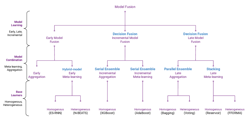
Figure 1: An taxonomy of model fusion. Showing Decision Fusion, Ensemble Learning, Stacking, and Hybrid-models, among others [9, 10].

This section examines meta-learning, model fusion and decision fusion as related concepts. It expands upon an existing taxonomy that previously jointly contextualised them [7]—first, a description of meta-learning within the context of time series forecasting. Next, decision fusion is described as it relates to forecasting and how it differs from traditional data fusion. Finally, ideas from the three areas; decision fusion, data fusion, and meta-learning; extended the existing taxonomy for model fusion. The expanded taxonomy allows us to analyse the proposed forecasting fusion techniques described in related work at the end of this section.

Consider models parameterised by data to improve performance on a task. These models are typical of machine learning, where an internal learning model is trained using data and a learning objective during base-model learning. These models are “base-learners” [11, 12, 12]. “Meta-learning” refers to techniques that learn a relationship between “meta-knowledge” (data and task characteristics) and the performance of the underlying base-learners. During meta-learning, an outer algorithm uses meta-knowledge to update the inner learning algorithm to improve the model on an outer learning objective [13]. In the context of time series, this process automatically acquires knowledge to select or fuse time series forecast models [14, 15].

Coincident with the above discussion, the word “fusion” refers to integrating information or knowledge from multiple sources. Fusion can, in some instances, be split into several sub-types: three of which are data fusion, feature fusion, and decision fusion [16]. Here the fusion approaches are classified according to the processing level at which the fusion occurs. These processing levels are termed early fusion or data-level fusion, late fusion or decision-level fusion, and intermediate fusion or feature-level fusion that combines late and early approaches [17].

Of these processing-level categories of fusion, decision fusion is aimed at learning to combine the beliefs of the collection of models into a single consensus belief [18]. Alternatively, one might say that decision fusion integrates the “decisions” of several base-learners into a single “decision” about a target [19]. This approach to “combining the wisdom of crowds” is also sometimes termed ensemble learning [20] and, in some studies, has been called “fusion models” [21, 22]. However, this view of fusion now excludes areas such as hybrid models and deep learning covered by meta-learning [23]. From a processing-level viewpoint of fusion, they are now categorised outside the boundaries of decision fusion.

Approaches with a processing-level view of fusion look to combine multi-modal, multi-resolution, and multi-temporal sources to produce more consistent, accurate, and valuable higher-level products [18]. Analogously, we are now positioned to take a learning view of fusion. Let us consider the definition of [7] for model fusion: “the integration of base-learners to produce a lower biased and variance; and a more robust, consistent, and accurate meta-model.” The presented taxonomy now sub-categorises model fusion along an axis based on whether the learning process is early, incremental, or late, with them being described as [7]:

integrates the base-learners before they have been parameterised (trained), and the combined model is trained as a single fused model.

first parameterises (pretrains) the base-learners individually. The base-learners are integrated into a single model without further modification.

performs model integration while parameterising (training) the base-learners one at a time. The already integrated base-learners’ parameters remain fixed once trained. However, the base-learner being incrementally added is trained during the integration step. The choice of the word “model” rather than “decision” is attributed to the fact that in the case of early model fusion, no decisions exist at the time of fusion. Decision fusion refers to only the incremental and late model fusion cases. One might argue that the correct term for early fusion is feature or data fusion. These terms are also valid but take a different processing-level view.

In the taxonomy for decision-fusion combiners by [19], we note that algorithms can be grouped into two distinct groups. The first group are those methods that use a simple aggregation scheme for combination. The second group is those that use more complex meta-learning. These groupings of combiners have previously been referred to by [24] as fixed or trained combiners. We are now in a position to explain the model-combining process of the taxonomy:

uses meta-learning to perform the model integration process (Trained Combiner).

[24], or Aggregation for short, uses a simple aggregation scheme, like averaging or voting, to perform the model integration (Fixed Combiner).

Finally, the nature of the base-learners needs to be considered. base-learners are sub-categorised as homogeneous if they come from the same hypothesis class (e.g. decision trees in a random forest or perceptrons in a neural network). If the base-learners come from different hypothesis classes (e.g. neural network and support vector machine), we would refer to them as heterogeneous [19].

Presenting the above discussion with some of the common pseudonyms for the classes of techniques allows us to arrive at the more complete taxonomy for model fusion shown in Figure 1. The following section reviews the relevant literature for forecasting model fusion in the presented taxonomy’s context.

II-A Related Work

One of the earliest examples of forecasting model fusion is by [25]. They introduce stacking as a late meta-learning fusion technique that selects one forecasting model among several based on the learnt performance for six-time series meta-features. [26] suggested that choosing a single model creates issues of model uncertainty and proposed using Bayesian model averaging instead. More recently, a more robust approach has been to set the weights using the predictions of heterogeneous base-learners using cross-validation instead of posterior probabilities [27]. [28] proposed increasing meta-features in the stacking approach by including recent statistics, such as linearity, curvature, stability, and entropy [29, 30, 8].

[9] studied late and incremental model fusion in forecasting time series. They compare the bagging, gradient-boosting, and stacking of base-learners. Their results suggest that boosting methods generally produce the lowest prediction errors. The top two submissions to the M4 forecasting competition supported these findings, also implementing ensemble learning.

The runner-up in the M4 Competition, FFORMA, uses late meta-learning fusion with heterogeneous base-learners. The stacking is implemented using extreme gradient boosting as the meta-learner. The meta-learner learns the weightings among several base-learners using meta-features extracted from the input time series [8]. The weightings learnt are then used to combine the models’ predictions as a feature-weighted average.

Hybrid models use early meta-learning with heterogeneous base-learners to achieve model fusion. They are the preferred family of fusion models and have retained traction in recent time series forecasting research [31, 32, 33, 34]. Hybrid models were initially proposed by Zhang [10] for forecasting, who showed that the fusion of the AutoRegressive Integrated Moving Average (ARIMA) and Multilayer Perceptron (MLP) models produces improved accuracy. Numerous hybrids implement Artificial Neural Networks (ANNs) or combine them with traditional models [35, 36, 37].

The Exponential Smoothing - Recurrent Neural Network (ES-RNN) is a hybrid forecasting model and winning submission of the M4 Competition. ES-RNN fuses a modified Holt-Winters and dilated Long Short Term Memory (LSTM) stacks [38] in early meta-learning using heterogeneous base-learners. As it stands, Neural Basis Expansion Analysis (N-BEATS) is a hybrid model that achieves SOTA forecasting accuracy by 3% over the ES-RNN [39]. N-BEATS is a hybrid forecasting method that integrates a fully connected neural network with traditional time series decomposition.

III Deep-learning FORecast Model Averaging (DeFORMA)

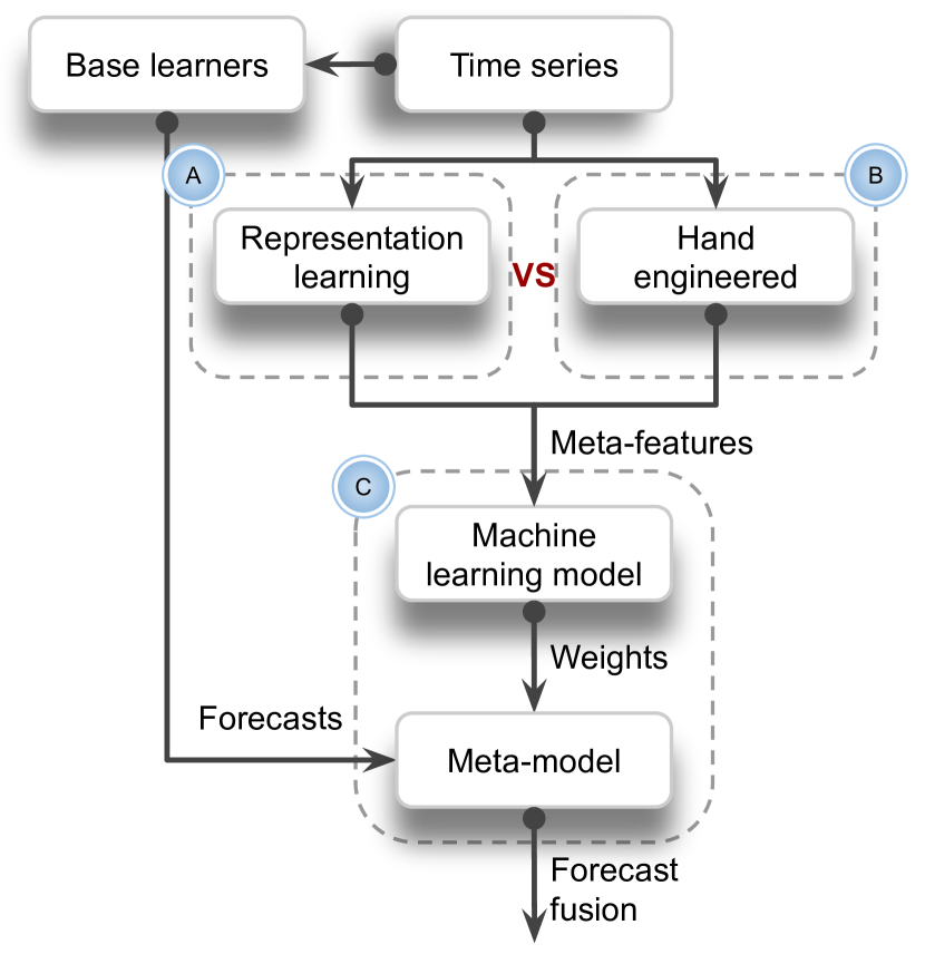
Figure 2: (A) DeFORMA versus (B) FFORMA approaches with respect to the (C) meta-learning. For DeFORMA, the Machine learning model is a fully connected neural network layer. For FFORMA, the Machine learning model is Gradient Boosting.

Much of the success of the hybrid models (ES-RNN,N-BEATS) stems from their ability to learn feature representations and use those representations in the model fusion process. Alternatively, FFORMA uses gradient boosting with the hand-engineered meta-features as input to weight heterogeneous base-learners’ forecasts. A natural question arises about the efficacy of using representation learning in a late meta-learning model such as FFORMA.

DeFORMA like FFORMA is a late meta-learning fusion method with heterogeneous base-learners. The distinction, seen in Figure 2, is that instead of using hand-engineered meta-features DeFORMA uses representing learning to learn meta-features from the data. To accomplish this, DeFORMA uses the same loss function

$$\sum_{i}^{\mathrm{\#Base-learners}}W_{i}F_{i}$$

as FFORMA, where $W_{i}$ are the weights learnt for each base-learner forecast $F_{i}$. DeFORMA replaces the gradient boosting model with a deep learning model. The remainder of this section discusses the neural network architecture and the resulting hyper-parameter choices.

III-A Neural Network Architecture

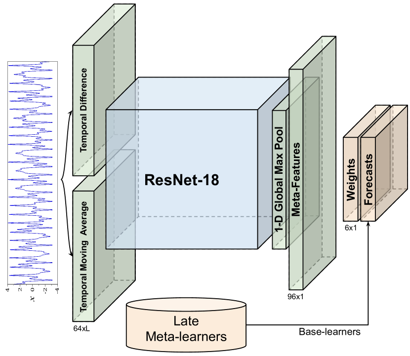
Figure 3: The DeFORMA architecture showing the modifications to the ResNet-18 backbone in green. Orange shows the components of the FFORMA loss.

At its core, DeFORMA uses a one-dimensional (1-D) ResNet-18 as the backbone, as seen in Figure 3. Researchers initially designed ResNet for images. Consequently, certain modifications are required. Firstly, all convolutions are replaced with 1D convolutions, and the global average pooling layer is replaced with a 1D global max pooling layer. Secondly, two Temporal heads are prepended to the input layer of the ResNet. The first Temporal head is a Differencing head. The second is a Moving Average head. More details descriptions of these Temporal heads are presented at the end of this sub-section. Finally, for short time series, the max pooling and two strides within the ResNet blocks for a deep neural network result in filters with a length of less than one. For this reason, the architecture limits the number of “halvings” (stride 2) that the ResNet blocks take.

The resulting architecture has the following hyper-parameters that require tuning: i) the number of halvings, ii) the number of convolutional filters, iii) the number of features in the output layer, iv) the maximum length of the time series and v) the dropout rate.

III-A1 Temporal Differencing Head

The Temporal Differencing head has as its primary purpose to remove seasonal trends. To achieve this, the head consists of three layers. The first layer is a 1-D convolution layer ($F\times L$) consisting of $F$ filters and having length $L$ (no bias). The length $L$ of the filters equals the seasonality$S+1$ of the time series. The weights of filters are constrained such that they must sum to zero. This convolution is followed by Layer Normalisation and then 1D Spatial Dropout.

III-A2 Temporal Moving Average Head

The Temporal Moving Average head has as its primary purpose to remove seasonality. To achieve this, the head consists of three layers. The first layer is a 1-D convolution layer ($F\times L$) consisting of $F$ filters and having length $L$ (no bias). The length $L$ of the filters is equal to the seasonality$S$ of the time series. The weights of filters are constrained such that they must sum to one. This convolution is followed by Layer Normalisation and then 1D Spatial Dropout.

IV Method

To test the primary hypothesis that learning the features required for FFORMA would be possible, the study empirically evaluated numerous SOTA models against the proposed solution. The accuracy of the forecast for this evaluation is assessed by measuring the mean and median Overall Weighted Average (OWA) on the M4 dataset. To this end, our experiment follows the procedure used by [7].

IV-A Dataset

Table I: Number of series per data frequency and domain [40].

Data subset	Micro	Industry	Macro	Finance	Demo- graphic	Other	Total
Yearly (Y)	6,538	3,716	3,903	6,519	1,088	1,236	23,000
Quarterly (Q)	6,020	4,637	5,315	5,305	1,858	865	24,000
Monthly (M)	10,975	10,017	10,016	10,987	5,728	277	48,000
Weekly (W)	112	6	41	164	24	12	359
Daily (D)	1,476	422	127	1,559	10	633	4,227
Hourly (H)	0	0	0	0	0	414	414
Total	25,121	18,798	19,402	24,534	8,708	3,437	100,000

Makridakis Competitions (or M-Competitions) establish an inventory of standard benchmark data sets that are the most convincing effort driving continuous advancement in forecasting techniques [41, 42]. The recent M4 Competition conducted a large-scale comparative study of $61$ forecasting methods. The comparison included statistical methods, for example, ARIMA and Holt-Winters, and machine learning methods, for example, MLP and Recurrent Neural Network (RNN). Similar to previous studies [40], they find that employing an incremental and late model fusion of base-learners delivers the most promising results [4, 5, 6]. Before the M5 competition, [41] suggested that machine learning models showed inferior forecasting performance overall. More recently, the M5 Competition was the first in the series with hierarchical time series data [42]. The M5 Competition confirmed late meta-learning fusion’s dominance in forecasting time series data. The top submissions were techniques that adopted parallel ensemble learning and gradient boosting, often with deep learning models as base-learners [43]. However, two early meta-learning hybrid models that use deep learning stand out, both of which have been SOTA results for M4: ES-RNN and N-BEATS.

[7] demonstrated that the results of the M5 competition are valid for the M4 competition. For this reason, this study focuses on the M4 Competition. The M4 dataset contains a $100,000$ time series of different seasonalities. The minimum time series length is as low as $13$ for the yearly series and $16$ for quarterly. Data are available on Github, and Table I provides a summary of the number of series per frequency and domain. Subset names H, D, W, M, Y and Q of Tables I - III correspond to the hourly, daily, weekly, monthly, yearly and quarterly seasonality subsets. Domains include economics, finance, demographics, industries, tourism, trade, labour and wages, real estate, transportation, natural resources and the environment.

IV-A1 Data Preprocessing

Little additional preprocessing is applied other than limiting the maximum length of input series as a requirement from TensorFlow. Further, if the time series is shorter than the maximum length, then zero padding is applied. The maximum length is treated as a hyperparameter. However, the ablation study shows that the proposed method is insensitive to this value.

IV-B Base-Learners

This section describes the base-learners used.

IV-B1 Auto-ARIMA

a classic approach for benchmarking forecast methods’ implementations. This study uses the forecasts from an Auto-ARIMA method that uses the maximum likelihood estimation to approximate the parameters [44].

IV-B2 Comb (or COMB S-H-D)

is the arithmetic average of three exponential smoothing methods: Single, Holt-Winters, and Damped exponential smoothing [45]. Comb was the winning approach for the M2 competition and was used as a benchmark in the M4 competition.

IV-B3 Theta

the most promising approach of the M3 competition [46]. Theta is a straightforward forecasting method that averages the extrapolated Theta lines, computed from two given Theta coefficients, applied to the second differences of the time series.

IV-B4 Damped Holt’s

is exponential smoothing with a trend component modified with a damping parameter $\phi$ imposed on the trend component [47, 48].

IV-B5 ES-RNN

is used as a base-learner and is described in more detail below [38].

IV-C Compared Forecasting Methods

This section describes the compared fusion models.

IV-C1 ES-RNN [38]

is a hybrid forecasting method. It produces more accurate forecasts using an early meta-learning fusion of homogeneous Exponential Smoothing (ES) base-learners with a LSTM meta-learner. ES-RNN was the top performing model of the M4 competition.

IV-C2 FFORMA [8]

adopts a feature-weighted model averaging strategy. A meta-learner, gradient boosting [49], learns to weight the effectiveness of a base-learner pool for different regions of a set of hand-engineered meta-features. The meta-learner then uses a late fusion of the predictions of the base-learners based on the learned weightings.

IV-C3 Feature-based FORecast Model Selection using Random Forest (FFORMS) [50]

was the precursor to FFORMA and used a random forest [51] for late meta-learning to select a single model from a pool of heterogeneous base-learners. The selection is based on their varying performance observed over the meta-data feature space. Following the original paper, the study used Gini impurity and the same meta-features as in FFORMA.

IV-C4 Feature-based FORecast Model Averaging using Neural Networks (FFORMA-N) [7]

uses a MLP for late meta-learning that takes the same meta-features as FFORMA as inputs and a one-hot encoded vector of the best-performing model as the model’s targets.

IV-C5 N-BEATS [39]

is a hybrid forecasting method that uses a MLP as a meta-learner with traditional time series decomposition blocks as base-learners.

IV-C6 Simple Model Averaging (AVG)

uses a simple model averaging as a baseline for comparison.

IV-D Experimental Setup

Figure 4: The proposed methodology integrates representation learning into the machine learning pipeline.

All comparisons are made using ten-fold cross-validation. Cross-validation is repeated five times, and scores are averaged over all 50 runs to rule out false positive results from random fluctuations. A pseudo-random number generator [52] is configured to produce the indices to split the data into training and validation sets for each of the five runs.

Figure 4 shows a more detailed view of the proposed methodology. The training and test splits are as per the M4 dataset. Base-learner forecasts are acquired from the M4 competition. The length of the training and testing target forecast horizons also follow the original M4 dataset.

IV-D1 Hyper-parameter Tuning

The architectures and hyper-parameters were all found using only the training set of the first fold of the first cross-validation run. Since our training and testing setup follows from  [7], the experiments in this study employ the hyper-parameters found in that study for FFORMA and its variants. The neural networks were tuned using backtesting, and the gradient boosting methods were tuned using Bayesian optimisation.

For DeFORMA, the architectures and hyper-parameters were also found using only the training set of the first fold of the first cross-validation run. The hyper-parameters were determined using a course grid search.

For model architecture, the hyper-parameters were selected from: i) Halvings - $[1,2,3,4,5]$, ii) Convolutional filters - $[64]$ iii) Meta-features - $[32,40,64,96,128]$ iv) Maximum length - $[32,64,96,128,160,192,224,256,288,320,352,384,416]$ and v) Dropout rate - $[0.1]$. Convolutional filters and Dropout rate corresponds to the default values for ResNet. Meta-features include the value of $40$ corresponding to the number of meta-features used by FFORMA.

For training, hyper-parameter values were selected from: i) Learning Rate - $[1e^{-3},1e^{-4},1e^{-5}]$ ii) Batch Size - $[92]$ iii) Epochs - $[150]$ iv) Early Stopping Patience - $[20]$ and v) Validation Set - $[10\%]$ of Training Set. The batch size was selected based on memory availability on the GPU. Epochs and patience were hand-tuned by evaluating training validation curves.

IV-E Analysis

The forecast horizon lengths for each frequency are six steps ahead for yearly data, eight steps ahead for quarterly data, $18$ steps ahead for monthly data, $13$ steps ahead for weekly data, $14$ steps ahead for daily data, and $48$ forecasts for hourly data. The M4 Competition uses OWA as a metric for comparison. The OWA, combines Symmetric Mean Absolute Percentage Error (sMAPE) [53] and the mean absolute scaled error Mean Absolute Scaled Error (MASE) [54]. The denominator and scaling factor of the MASE formula are the in-sample mean absolute error from one-step-ahead predictions of the Naïve model $2$, and $n$ is the number of data points.

IV-F Tools and Libraries

All algorithms were implemented in Python and ran on a mixture of Intel and AMD chips using NVIDIA GPUs. The libraries include a mix of TensorFlow, Scikit Learn and LightGBM. The source code of our experiments is available on GitHub .

V Results and Discussion

Table II: Mean OWA errors on the M4 test set and Schulze Rank $\downarrow$ [55]. Bold is best, and grey is second best.

	H (0.4K)	D (4.2K)	W (0.4K)	M (48K)	Y (23K)	Q (24K)	$\downarrow$
AVG	0.847	0.985	0.860	0.863	0.804	0.856	8
ES-RNN	0.440	1.046	0.864	0.836	0.778	0.847	7
FFORMS	0.423	0.981	0.740	0.817	0.752	0.830	4
N-BEATS$\dagger$	0.464	0.974	0.703	0.819	0.758	0.800	4
FFORMA-N	0.428	0.979	0.718	0.813	0.746	0.828	3
FFORMA	0.415	0.983	0.725	0.800	0.732	0.816	2
DeFORMA$\ddagger$	0.423	0.972	0.700	0.802	0.729	0.810	1
$\dagger$ transcribed for comparison [39, 56].
$\ddagger$ proposed methods.

The results presented in this section shed light on the comparison between using representation learning and hand-engineered features for forecast model fusion. The study aimed to evaluate if using representation learning could improve on FFORMA and how the proposed method might compare to other SOTA results when considering mean and median OWA. Table II shows the mean OWA for comparing the selected fusion methods. The table also shows the compared methods ranked by the Schulze rank. The grey backgrounds are the two best performers, with the top result in bold. The median results are presented alongside the Schulze rank across all the different seasonalities.

The results support the claim that DeFORMA outperforms the original FFORMA. Both DeFORMA and FFORMA improve on ES-RNN and N-BEATS. Interestingly in Table II where FFORMA-N had previously been the SOTA for Daily (D) and Weekly (W), the analysis shows that DeFORMA now outperforms the others. This result is surprising since representation learning is expected to be data-hungry. The suspicion is that the lower data requirements would allow FFORMA to dominate in these areas. When considering the Schulze ranking, the results support the notion that DeFORMA is the overall best-performing model.

When considering the original FFORMA, it is clear from [7] that late meta-learning using heterogeneous base-learners is a promising approach to model fusion. However, the same study observed that FFORMA-N and even AVG could outperform some smaller subsets. N-BEATS and ES-RNN are also competitive for specific subsets of data, probably due to the representation learning they can affect. DeFORMA combines the benefits of representation learning from N-BEATS and ES-RNN together with the output layer of FFORMA-N to allow for representation learning in a late meta-learning model fusion algorithm. The results are conclusive as to the efficacy of this approach.

V-A Ablations

Table III: Median OWA errors on the M4 test set. Bold is best, and grey is second best.

	H (0.4K)	D (4.2K)	W (0.4K)	M (48K)	Y (23K)	Q (24K)
FFORMA	0.318	0.723	0.529	0.602	0.491	0.580
FFORMA-N	0.326	0.720	0.539	0.614	0.508	0.594
DeFORMA‡	0.330	0.711	0.525	0.603	0.491	0.576
DeFORMA(224)	0.342	0.708	0.517	0.602	0.499	0.575
$\ddagger$ proposed methods.

The results in Table III show the median OWA for DeFORMA (224). In this instance, the hyper-parameter for time series length was left at the original $224$ of ResNet-18 and all halvings and filters as per the original architecture. The results show the robustness of DeFORMA to these hyper-parameters.

The experiments were also completed using data augmentation, which led to no improvement and VGG-11, which also led to no improvements in the results. The hyper-parameter selection for the number of meta-features learned impacted the results. Finally, excluding both or one of the Temporal Heads led to a significant drop in performance across all experiments.

VI Conclusion

The study sought to compare a representation learning late meta-learning model fusion approach to several other methods and to provide a complete taxonomy for the discussion of forecast model fusion. The results demonstrate that the proposed method, DeFORMA, is, in fact, SOTA for the M4 dataset. These results are noteworthy since using representing learning overcomes the need for hand-engineering features. It is worth considering that the results are applied in a univariate setting and, as such, will need further work to confirm them in the hierarchical and multivariate settings. Given that representation learning is effective, the next question is whether transfer learning can be applied in this setting across seasonalities.

References

- [1] David H Wolpert and William G Macready “No free lunch theorems for optimization” In IEEE transactions on evolutionary computation 1.1 IEEE, 1997, pp. 67–82
- [2] Christopher M Bishop and Nasser M Nasrabadi “Pattern recognition and machine learning” Springer, 2006
- [3] DJ Reid “A comparison of forecasting techniques on economic time series” In Forecasting in Action. Operational Research Society and the Society for Long Range Planning Operational Research Society, 1972
- [4] Nicholas G Reich et al. “A collaborative multiyear, multimodel assessment of seasonal influenza forecasting in the United States” In Proceedings of the National Academy of Sciences 116.8 National Acad Sciences, 2019, pp. 3146–3154
- [5] Craig J McGowan et al. “Collaborative efforts to forecast seasonal influenza in the United States, 2015–2016” In Scientific reports 9.1 Nature Publishing Group, 2019, pp. 1–13
- [6] Michael A Johansson et al. “An open challenge to advance probabilistic forecasting for dengue epidemics” In Proceedings of the National Academy of Sciences 116.48 National Acad Sciences, 2019, pp. 24268–24274
- [7] Pieter Cawood and Terence Zyl “Evaluating State of the Art, Forecasting Ensembles-and Meta-learning Strategies for Model Fusion” In Forecasting 4 MDPI, 2022, pp. 732–751
- [8] Pablo Montero-Manso, George Athanasopoulos, Rob J Hyndman and Thiyanga S Talagala “FFORMA: Feature-based forecast model averaging” In International Journal of Forecasting 36.1 Elsevier, 2020, pp. 86–92
- [9] Matheus Henrique Dal Molin Ribeiro and Leandro Santos Coelho “Ensemble approach based on bagging, boosting and stacking for short-term prediction in agribusiness time series” In Applied Soft Computing 86 Elsevier, 2020, pp. 105837
- [10] G Peter Zhang “Time series forecasting using a hybrid ARIMA and neural network model” In Neurocomputing 50 Elsevier, 2003, pp. 159–175
- [11] Ricardo Vilalta, Christophe G Giraud-Carrier, Pavel Brazdil and Carlos Soares “Using Meta-Learning to Support Data Mining.” In Int. J. Comput. Sci. Appl. 1.1, 2004, pp. 31–45
- [12] Xiaozhe Wang, Kate Smith-Miles and Rob Hyndman “Rule induction for forecasting method selection: Meta-learning the characteristics of univariate time series” In Neurocomputing 72.10-12 Elsevier, 2009, pp. 2581–2594
- [13] Timothy Hospedales, Antreas Antoniou, Paul Micaelli and Amos Storkey “Meta-learning in neural networks: A survey” In IEEE transactions on pattern analysis and machine intelligence 44.9 IEEE, 2021, pp. 5149–5169
- [14] Ricardo Prudêncio and Teresa Ludermir “Using machine learning techniques to combine forecasting methods” In AI 2004: Advances in Artificial Intelligence: 17th Australian Joint Conference on Artificial Intelligence, Cairns, Australia, December 4-6, 2004. Proceedings 17, 2005, pp. 1122–1127 Springer
- [15] Christiane Lemke and Bogdan Gabrys “Meta-learning for time series forecasting and forecast combination” In Neurocomputing 73.10-12 Elsevier, 2010, pp. 2006–2016
- [16] Belur V Dasarathy “Sensor fusion potential exploitation-innovative architectures and illustrative applications” In Proceedings of the IEEE 85.1 IEEE, 1997, pp. 24–38
- [17] Daniel Michelsanti et al. “An overview of deep-learning-based audio-visual speech enhancement and separation” In IEEE/ACM Transactions on Audio, Speech, and Language Processing 29 IEEE, 2021, pp. 1368–1396
- [18] Abhijit Sinha et al. “Estimation and decision fusion: A survey” In Neurocomputing 71.13-15 Elsevier, 2008, pp. 2650–2656
- [19] Cheng Zhang, Nilam NA Sjarif and Roslina B Ibrahim “Decision Fusion for Stock Market Prediction: A Systematic Review” In IEEE Access IEEE, 2022
- [20] Ian Goodfellow, Yoshua Bengio and Aaron Courville “Deep learning” MIT press, 2016
- [21] Deepika Nalabala and Mundukur Nirupamabhat “Financial Predictions based on Fusion Models-A Systematic Review” In 2021 International Conference on Emerging Smart Computing and Informatics (ESCI), 2021, pp. 28–37 IEEE
- [22] Ankit Thakkar and Kinjal Chaudhari “Fusion in stock market prediction: a decade survey on the necessity, recent developments, and potential future directions” In Information Fusion 65 Elsevier, 2021, pp. 95–107
- [23] Tom Schaul and Jürgen Schmidhuber “Metalearning” In Scholarpedia 5.6, 2010, pp. 4650
- [24] Moacir P Ponti Jr “Combining classifiers: from the creation of ensembles to the decision fusion” In 2011 24th SIBGRAPI Conference on Graphics, Patterns, and Images Tutorials, 2011, pp. 1–10 IEEE
- [25] B Arinze “Selecting appropriate forecasting models using rule induction” In Omega 22.6 Elsevier, 1994, pp. 647–658
- [26] Adrian E Raftery, David Madigan and Jennifer A Hoeting “Bayesian model averaging for linear regression models” In Journal of the American Statistical Association 92.437 Taylor & Francis, 1997, pp. 179–191
- [27] Bertrand Clarke “Comparing Bayes model averaging and stacking when model approximation error cannot be ignored” In Journal of Machine Learning Research 4.Oct, 2003, pp. 683–712
- [28] Pieter Cawood and Terence L. Zyl “Feature-Weighted Stacking for Nonseasonal Time Series Forecasts: A Case Study of the COVID-19 Epidemic Curves” In 2021 8th International Conference on Soft Computing Machine Intelligence (ISCMI), 2021, pp. 53–59
- [29] Ana C Lorena et al. “Data complexity meta-features for regression problems” In Machine Learning 107.1 Springer, 2018, pp. 209–246
- [30] Sasan Barak, Mahdi Nasiri and Mehrdad Rostamzadeh “Time series model selection with a meta-learning approach; evidence from a pool of forecasting algorithms” In arXiv preprint arXiv:1908.08489, 2019
- [31] Nian Liu et al. “A hybrid forecasting model with parameter optimization for short-term load forecasting of micro-grids” In Applied Energy 129 Elsevier, 2014, pp. 336–345
- [32] Jian-Zhou Wang, Yun Wang and Ping Jiang “The study and application of a novel hybrid forecasting model–A case study of wind speed forecasting in China” In Applied Energy 143 Elsevier, 2015, pp. 472–488
- [33] Yong Qin et al. “Hybrid forecasting model based on long short term memory network and deep learning neural network for wind signal” In Applied energy 236 Elsevier, 2019, pp. 262–272
- [34] Gitanjali R Shinde et al. “Forecasting models for coronavirus disease (COVID-19): a survey of the state-of-the-art” In SN Computer Science 1.4 Springer, 2020, pp. 1–15
- [35] Thabang Mathonsi and Terence L Zyl “Prediction interval construction for multivariate point forecasts using deep learning” In 2020 7th International Conference on Soft Computing & Machine Intelligence (ISCMI), 2020, pp. 88–95 IEEE
- [36] Siddeeq Laher, Andrew Paskaramoorthy and Terence L Van Zyl “Deep Learning for Financial Time Series Forecast Fusion and Optimal Portfolio Rebalancing” In 2021 IEEE 24th International Conference on Information Fusion (FUSION), 2021, pp. 1–8 IEEE
- [37] Thabang Mathonsi and Terence L Zyl “A Statistics and Deep Learning Hybrid Method for Multivariate Time Series Forecasting and Mortality Modeling” In Forecasting 4.1 Multidisciplinary Digital Publishing Institute, 2022, pp. 1–25
- [38] Slawek Smyl “A hybrid method of exponential smoothing and recurrent neural networks for time series forecasting” M4 Competition In International Journal of Forecasting 36.1, 2020, pp. 75–85
- [39] Boris N Oreshkin, Dmitri Carpov, Nicolas Chapados and Yoshua Bengio “N-BEATS: Neural basis expansion analysis for interpretable time series forecasting” In arXiv preprint arXiv:1905.10437, 2019
- [40] Spyros Makridakis, Evangelos Spiliotis and Vassilios Assimakopoulos “The M4 Competition: 100,000 time series and 61 forecasting methods” In International Journal of Forecasting 36.1 Elsevier, 2020, pp. 54–74
- [41] Spyros Makridakis, Rob J Hyndman and Fotios Petropoulos “Forecasting in social settings: The state of the art” In International Journal of Forecasting 36.1 Elsevier, 2020, pp. 15–28
- [42] Spyros Makridakis, Evangelos Spiliotis and Vassilios Assimakopoulos “The M5 competition: Background, organization, and implementation” In International Journal of Forecasting Elsevier, 2021
- [43] Spyros Makridakis, Evangelos Spiliotis and Vassilios Assimakopoulos “M5 accuracy competition: Results, findings, and conclusions” In International Journal of Forecasting Elsevier, 2022
- [44] Rob J Hyndman and Yeasmin Khandakar “Automatic time series forecasting: the forecast package for R” In Journal of statistical software 27.1, 2008, pp. 1–22
- [45] Spyros Makridakis and Michele Hibon “The M3-Competition: results, conclusions and implications” In International journal of forecasting 16.4 Elsevier, 2000, pp. 451–476
- [46] Vassilis Assimakopoulos and Konstantinos Nikolopoulos “The theta model: a decomposition approach to forecasting” In International journal of forecasting 16.4 Elsevier, 2000, pp. 521–530
- [47] Charles C Holt “Forecasting seasonals and trends by exponentially weighted moving averages” In International journal of forecasting 20.1 Elsevier, 2004, pp. 5–10
- [48] Eddie McKenzie and Everette S Gardner Jr “Damped trend exponential smoothing: a modelling viewpoint” In International Journal of Forecasting 26.4 Elsevier, 2010, pp. 661–665
- [49] Tianqi Chen and Carlos Guestrin “Xgboost: A scalable tree boosting system” In Proceedings of the 22nd acm sigkdd international conference on knowledge discovery and data mining, 2016, pp. 785–794
- [50] Thiyanga S Talagala, Rob J Hyndman and George Athanasopoulos “Meta-learning how to forecast time series” In Monash Econometrics and Business Statistics Working Papers 6 Monash University, Department of EconometricsBusiness Statistics, 2018, pp. 18
- [51] Andy Liaw and Matthew Wiener “Classification and regression by randomForest” In R news 2.3, 2002, pp. 18–22
- [52] Lenore Blum, Manuel Blum and Mike Shub “A simple unpredictable pseudo-random number generator” In SIAM Journal on computing 15.2 SIAM, 1986, pp. 364–383
- [53] Spyros Makridakis “Accuracy measures: theoretical and practical concerns” In International journal of forecasting 9.4 Elsevier, 1993, pp. 527–529
- [54] Rob J Hyndman and Anne B Koehler “Another look at measures of forecast accuracy” In International journal of forecasting 22.4 Elsevier, 2006, pp. 679–688
- [55] Markus Schulze “A new monotonic, clone-independent, reversal symmetric, and condorcet-consistent single-winner election method” In Social choice and Welfare 36.2 Springer, 2011, pp. 267–303
- [56] Sebastian Zeng, Florian Graf, Christoph Hofer and Roland Kwitt “Topological attention for time series forecasting” In Advances in Neural Information Processing Systems 34, 2021, pp. 24871–24882